Numerical Investigation of Fractional-Order Swift–Hohenberg Equations via a Novel Transform

Abstract

In this paper, the Elzaki transform decomposition method is implemented to solve the time-fractional Swift–Hohenberg equations. The presented model is related to the temperature and thermal convection of fluid dynamics, which can also be used to explain the formation process in liquid surfaces bounded along a horizontally well-conducting boundary. In the Caputo manner, the fractional derivative is described. The suggested method is easy to implement and needs a small number of calculations. The validity of the presented method is confirmed from the numerical examples. Illustrative figures are used to derive and verify the supporting analytical schemes for fractional-order of the proposed problems. It has been confirmed that the proposed method can be easily extended for the solution of other linear and non-linear fractional-order partial differential equations.

1. Introduction

The concept of Fractional Calculus (FC) is old, which arises from the nth derivative notation used by Leibniz in their publication. So, L’Hopital asks Leibniz what the result would be if the order is non-integer [1]. Riemann and Liouville defined the concept of fractional order differentiation in the 19th century. Later on, researchers began to research FC and found that fractional-order models are more suitable than integer-order models for some real-world problems [2,3,4]. FC is an efficient and powerful tool for describing memory and hereditary properties in various materials and processes.

Fractional Differential Equations (FDEs) have significantly gained much attention from researchers due to providing fractional modeling of different phenomena in nature. Due to this reason, the implementation of FDEs to model different physical systems and processes has been increased, for example, colored noise [5], economics [6], oscillation of earthquake [7], and bioengineering [8]. The other applications are control theory [9], rheology [10], visco-elastic materials [11], signal processing [12], damping method [13], polymers [14], and so on. The scheme consisting of integer partial differential equations and fractional-order partial differential equations with the fractional Caputo derivative has a well-designed symmetry structure. This problem is utilized to analyze dispersive wave phenomena in different areas of applied science, like quantum mechanics and plasma physics. Nonlinear phenomena play a crucial role in applied mathematics and physics; we know that most engineering problems are non-linear, and solving them analytically is difficult. In physics and mathematics, obtaining exact or approximate solutions to nonlinear FPDEs is still a significant problem that requires new methods to discover exact or approximate solutions.

Because of the above fact, researchers have developed numerous numerical and analytical techniques for the solution of FPDEs [15,16]. In [17], A.A. Alderremy et al. used Modified Reduced Differential Transform Method (MRDTM) to solve the fractional nonlinear Newell–Whitehead–Segel equation. M.S. Rawashdeh and H. Al-Jammal [18] implemented the fractional natural decomposition method (FNDM) for finding approximate analytical solutions to systems of nonlinear PDEs. Certain analytical solutions of the fractional-order diffusion equations were found by K. Shah et al. [19], who used Natural Transform Method (NTM). To obtain the approximate and exact solutions of space and time-fractional Burgers equations with initial conditions [20], M. Inc implemented a variational iteration method.

In [21], using the approximate analytical method, travelling wave solutions for Korteweg-de Vries equations having fractional-order were discussed. Similarly, in [22], F.A. Alawad et al. solved space-time fractional telegraph equations using a new technique of the Laplace variational iteration method. H. Jafari et al. [23] found the approximate solution of the nonlinear gas dynamic equation by implementing homotopy analysis method. To obtain a series form solution of time-fractional coupled Burgers equations. P. Veereshaa and D.G. Prakash used a reliable technique q-homotopy analysis transform method (q-HATM) [24]. In [25], L. Yan used the iterative Laplace transform method, which combines two methods, the iterative method, and the Laplace transform method, to obtain the numerical solutions of fractional Fokker–Planck equations.

However, we used a new technique formed by the combination of Elzaki transform [26] and the Adomian decomposition method [27,28] known as the Elzaki Transform Decomposition Method (ETDM). The Elzaki transformation is renowned for handling linear ordinary differential equations, linear partial differential equations, and integral equations, as seen in [29,30,31]. In contrast, the Adomian decomposition method [27,28] is a well-known method for handling linear and nonlinear, homogeneous and nonhomogeneous differential and partial differential equations, integro-differential, and FDEs series form solution.

In this paper, we aim to solve Swift–Hohenberg (S-H) equation with the help of ETDM. The S-H equation was first introduced and derived from the equations for thermal convection by J. Swift and P. Hohenberg [32]. The general form of the S-H equation is

$$\frac{{\partial }^{\delta }\rho }{\partial {\tau }^{\delta }}=b\rho -\left(1+\frac{{\partial }^2}{\partial {\tau }^2}\right)\rho -N\left(\rho \right),b\in \mathbb{R},0<\delta \le 1,$$

(1)

where $\rho$ is a scalar function, b is the real constant, and $N\left(\rho \right)$ is a nonlinear term. The S-H equation has many applications in engineering and science, such as physics, biology, laser study fluid, and hydro-dynamics [33,34,35]. The S-H equation plays an important role in pattern formation theory in fluid layers confined between horizontal well-conducting boundaries [36]. This equation has many applications in the modeling pattern formation and its different issues, including the selection of pattern, effects of noise on bifurcations, the dynamics of defects, and spatiotemporal chaos [37,38,39,40].

2. Preliminaries

In this subsection, we recall some simple and most significant concepts concerning fractional calculus.

Definition 1

([41,42,43]). Abel-Riemann (A-R) described $D^{\delta }$ operator of the δ order as

$$D^{\delta }\rho \left(\psi \right)=\left\{\begin{array}{cc}{\displaystyle \frac{d^n}{d{\psi }^n}\rho \left(\psi \right),}\hfill & \delta =n;\hfill \\ {\displaystyle \frac{1}{\Gamma (n-\delta )}\frac{d}{d{\psi }^n}{\int }_0^{\psi }\frac{\rho \left(\mathcal{T}\right)}{{(\psi -\tau )}^{\delta -n+1}}d\tau ,}\hfill & n-1<\delta <n,\hfill \end{array}\right.$$

(2)

where $\delta \in {\mathbb{R}}^{+},n\in {\mathbb{Z}}^{+}$ and

$$D^{-\delta }\rho \left(\psi \right)=\frac{1}{\Gamma \left(\delta \right)}{\int }_0^{\psi }{(\psi -\tau )}^{\delta -1}\rho \left(\tau \right)d\tau ,0<\delta \le 1.$$

(3)

Definition 2

([42,43]). The fractional order A-R integral operator $J^{\delta }$ is given as

$$J^{\delta }\rho \left(\psi \right)=\frac{1}{\Gamma \left(\delta \right)}{\int }_0^{\psi }{(\psi -\tau )}^{\delta -1}\rho \left(\tau \right)d\tau ,\tau >0,\delta >0.$$

(4)

By Podlubny [42] we may have

$$\begin{array}{cc}\hfill J^{\delta }{\tau }^n& =\frac{\Gamma (n+1)}{\Gamma (n+\delta +1)}{\tau }^{n+\delta },\hfill \end{array}$$

(5)

$$\begin{array}{cc}\hfill D^{\delta }{\tau }^n& =\frac{\Gamma (n+1)}{\Gamma (n-\delta +1)}{\tau }^{n-\delta }.\hfill \end{array}$$

(6)

Definition 3

([41,42,44,45]). In the Caputo manner, the operator $D^{\delta }$ with the order δ is given as

$$D^{\delta }\rho \left(\psi \right)=\left\{\begin{array}{cc}{\displaystyle \frac{1}{\Gamma (n-\delta )}{\int }_0^{\psi }\frac{{\rho }^n\left(\tau \right)}{{(\psi -\tau )}^{\delta -n+1}}d\tau ,}\hfill & n-1<\delta <n;\hfill \\ {\displaystyle \frac{d^n}{d{\tau }^n}\rho \left(\psi \right),}\hfill & \delta =n\hfill \end{array}\right.$$

(7)

with the following properties:

$$\begin{array}{cc}\hfill & \left(a\right)D_{\tau }^{\delta }{J}_{\tau }^{\delta }f\left(\tau \right)=f\left(\tau \right);\hfill \\ \hfill & \left(b\right)J_{\tau }^{\delta }{D}_{\tau }^{\delta }f\left(\tau \right)=f\left(\tau \right)-\sum _{k=0}^n{f}^k\left(0^{+}\right)\frac{{\tau }^k}{k!}\hfill \end{array}$$

(8)

for $\tau >0$ and $n-1<\delta \le n,n\in \mathbb{N}$.

Definition 4

([46]). The Mittag–Leffler function ψ is defined as

$$E_{\delta }\left(\psi \right)=\sum _{k=0}^{\infty }\frac{{\psi }^k}{\Gamma (\delta k+1)},\delta >0.$$

(9)

For a $f\left(t\right)$ function, the ET or modified Sumudu transform definition is given as

$$E\left[f\left(\tau \right)\right]=F\left(r\right)=r{\int }_0^{\infty }h\left(\tau \right)e^{\frac{-\tau }{r}}d\tau ,r>0.$$

(10)

The transformation of Elzaki is a very useful and powerful tool for solving the integral equation that can not be solved by the Sumudu transformation method.

The following ET transformations of partial derivatives, which can be obtained by using integration by parts, may be used in (8):

• ${\displaystyle E[\frac{\partial f(\psi ,\tau )}{\partial \tau }]=\frac{1}{r}F(\psi ,r)-rf(\psi ,0).}$
• ${\displaystyle E[\frac{{\partial }^{2}f(\psi ,\tau )}{\partial {\tau }^2}]=\frac{1}{r^2}F(\psi ,r)-f(\psi ,0)-r\frac{\partial f(\psi ,0)}{\partial \tau }.}$
• ${\displaystyle E[\frac{\partial f(\psi ,\tau )}{\partial \psi }]=\frac{d}{d\psi }F(\psi ,r).}$
• ${\displaystyle E[\frac{{\partial }^{2}f(\psi ,\tau )}{\partial {\psi }^2}]=\frac{d^2}{d{\psi }^2}F(\psi ,r).}$

Theorem 1

([47]). Let $U\left(s\right)$ be the Laplace transform of $f\left(\tau \right)$ then ET $F\left(r\right)$ of $f\left(\tau \right)$ is specified as

$$F\left(r\right)=rU(\frac{1}{r}).$$

(11)

Theorem 2

([47]). If $F\left(r\right)$ is the ET of the $f\left(\tau \right)$ function, then

$$E\left[D^{\delta }f\left(\tau \right)\right]=\frac{F\left(r\right)}{r^{\delta }}-\sum _{k=0}^{n-1}{r}^{k-\delta +2}f(k)\left(0\right),n-1<\delta \le n.$$

(12)

3. Idea of ETDM

The ETDM solution for fractional partial differential equations is described in this section.

$$D_{\tau }^{\delta }\rho (\psi ,\tau )+{\overline{\mathcal{G}}}_1\rho (\psi ,\tau )+{\mathcal{N}}_1\rho (\psi ,\tau )-{\mathcal{P}}_1(\psi ,\tau )=0,n-1<\delta \le n$$

(13)

with initial conditions

$$\rho (\psi ,0)=g_1\left(\psi \right),$$

(14)

where $D_{\tau }^{\delta }=\frac{{\partial }^{\delta }}{\partial {\tau }^{\delta }}$ is the fractional derivative in Caputo sense having order $\delta$, ${\overline{\mathcal{G}}}_1$ and ${\mathcal{N}}_1$ are linear and non-linear functions, respectively, and source operator is ${\mathcal{P}}_1$.

By applying Elzaki transform on both sides of (13), we obtain

$$E\left[D_{\tau }^{\delta }\rho (\psi ,\tau )\right]+E[{\overline{\mathcal{G}}}_1\rho (\psi ,\tau )+{\mathcal{N}}_1\rho (\psi ,\tau )-{\mathcal{P}}_1(\psi ,\tau )]=0.$$

(15)

By Elzaki transform property of differentiation, we get

$$\begin{array}{cc}\hfill E\left[\rho (\psi ,\tau )\right]& =s^{\delta }\sum _{k=0}^{m-1}{s}^{2+k-\delta }\frac{{\partial }^k\rho (\psi ,\tau )}{{\partial }^k\tau }{|}_{\tau =0}\hfill \\ \hfill & +s^{\delta }E\left[{\mathcal{P}}_1(\psi ,\tau )\right]-s^{\delta }E\{{\overline{\mathcal{G}}}_1\rho (\psi ,\tau )+{\mathcal{N}}_1\rho (\psi ,\tau )\}].\hfill \end{array}$$

(16)

ETDM determines the solution of the infinite sequence of $\rho (\psi ,\tau )$

$$\rho (\psi ,\tau )=\sum _{m=0}^{\infty }{\rho }_m(\psi ,\tau ).$$

(17)

The decomposition of nonlinear terms by Adomian polynomials ${\mathcal{N}}_1$ is defined as

$${\mathcal{N}}_1\rho (\psi ,\tau )=\sum _{m=0}^{\infty }{\mathcal{A}}_m.$$

(18)

The Adomian polynomials can represent all forms of nonlinearity as

$${\mathcal{A}}_m=\frac{1}{m!}{\left[\frac{{\partial }^m}{\partial {\ell }^m}\left\{{\mathcal{N}}_1\left(\sum _{k=0}^{\infty }{\ell }^k{\psi }_k,\sum _{k=0}^{\infty }{\ell }^k{\tau }_k\right)\right\}\right]}_{\ell =0}.$$

(19)

Putting (17) and (19) into (16), gives

$$\begin{array}{cc}\hfill & E\left[\sum _{m=0}^{\infty }{\rho }_m(\psi ,\tau )\right]=s^{\delta }\sum _{k=0}^{m-1}{s}^{2+k-\delta }\frac{{\partial }^k\rho (\psi ,\tau )}{{\partial }^k\tau }{|}_{\tau =0}+s^{\delta }E\hfill \\ \hfill & \left\{{\mathcal{P}}_1(\psi ,\tau )\right\}-s^{\delta }E\left\{{\overline{\mathcal{G}}}_1\rho (\sum _{m=0}^{\infty }{\psi }_m,\sum _{m=0}^{\infty }{\tau }_m)+\sum _{m=0}^{\infty }{\mathcal{A}}_m\right\}.\hfill \end{array}$$

(20)

By applying inverse Elzaki to (20), we obtain

$$\begin{array}{cc}\hfill & \sum _{m=0}^{\infty }{\rho }_m(\psi ,\tau )=E^{-}\left[s^{\delta }\sum _{k=0}^{m-1}{s}^{2+k-\delta }\frac{{\partial }^k\rho (\psi ,\tau )}{{\partial }^k\tau }{|}_{\tau =0}+s^{\delta }E\right.\hfill \\ \hfill & \left.\left\{{\mathcal{P}}_1(\psi ,\tau )\right\}-s^{\delta }E\left\{{\overline{\mathcal{G}}}_1\rho \left(\sum _{m=0}^{\infty }{\psi }_m,\sum _{m=0}^{\infty }{\tau }_m\right)+\sum _{m=0}^{\infty }{\mathcal{A}}_m\right\}\right].\hfill \end{array}$$

(21)

The following terms are described as

$$\begin{array}{cc}\hfill & {\rho }_0(\psi ,\tau )=E^{-}\left[s^{\delta }\sum _{k=0}^{m-1}{s}^{2+k-\delta }\frac{{\partial }^k\rho (\psi ,\tau )}{{\partial }^k\tau }{|}_{\tau =0}+s^{\delta }{E}^{+}\left\{{\mathcal{P}}_1(\psi ,\tau )\right\}\right],\hfill \\ \hfill & {\rho }_1(\psi ,\tau )=-E^{-}\left[s^{\delta }{E}^{+}\{{\overline{\mathcal{G}}}_1\rho ({\psi }_0,{\tau }_0)+{\mathcal{A}}_0\}\right],\hfill \end{array}$$

(22)

for $m\ge 1$, is determined as

$${\rho }_{m+1}(\psi ,\tau )=-E^{-}\left[s^{\delta }{E}^{+}\{{\overline{\mathcal{G}}}_1\rho ({\psi }_m,{\tau }_m)+{\mathcal{A}}_m\}\right].$$

(23)

4. Existence and Uniqueness Results for ETDM

In what follows, we will demonstrate that the sufficient conditions assure the existence of a unique solution. Our desired existence of solutions in the case of SDM follows by [40].

Theorem 3.

(Uniqueness theorem): Equation (23) has a unique solution whenever $0<ϵ<1,$ where $ϵ=\frac{({\check{L}}_1+{\check{L}}_2+{\check{L}}_3){\tau }^{(\delta -1)}}{\delta !}.$

Proof. 

Assume that $M=\left(\mathcal{C}\left[I\right],\parallel .\parallel \right)$ represents all continuous mappings on the Banach space, defined on $I=[0,\mathbb{T}]$ having the norm $\parallel .\parallel .$ For this we introduce a mapping $W:M\mapsto M,$ we have

$${\rho }_{n+1}(\psi ,\tau )=\rho (\psi ,\tau )+E^{-1}\left[{\left(\frac{\omega }{\xi }\right)}^{\delta }E\right[\mathcal{L}\left[{\rho }_n(\psi ,\tau )\right]+\mathcal{R}[{\rho }_n(\psi ,\tau )]+\mathcal{N}[{\rho }_n(\psi ,\tau )]\left]\right],n\ge 0,$$

(24)

where $\mathcal{L}\left[\rho (\psi ,\tau )\right]\equiv \frac{{\partial }^3\rho (\psi ,\tau )}{\partial {\psi }^2}$ and $\mathcal{R}\left[\rho (\psi ,\tau )\right]\equiv \frac{\partial \rho (\psi ,\tau )}{\partial \psi }.$ Now assume that $\mathcal{L}\left[\rho (\psi ,\tau )\right]$ and $\mathcal{M}\left[\rho (\psi ,\tau )\right]$ are also Lipschitzian with $|\mathcal{R}\rho -\mathcal{R}\check{\rho }|<{\check{L}}_1|\rho -\check{\rho }|$ and $|\mathcal{L}\rho -\mathcal{L}\check{\rho }|<{\check{L}}_2|\rho -\check{\rho }|,$ where ${\check{L}}_1$ and ${\check{L}}_2$ are Lipschitz constant, respectively, and $\rho ,\check{\rho }$ are various values of the mapping.

$$\begin{array}{cc}\hfill \parallel W\rho -W\check{\rho }\parallel & =\underset{\tau \in I}{max}\left|\begin{array}{c}{E}^{-1}\left[s^{\delta }E\right[\mathcal{L}\left[\rho (\psi ,\tau )\right]+\mathcal{R}\left[\rho (\psi ,\tau )\right]+\mathcal{N}\left[\rho (\psi ,\tau )\right]\left]\right]\hfill \\ \hspace{1em}-E^{-1}\left[s^{\delta }E\right[\mathcal{L}\left[\check{\rho }(\psi ,\tau )\right]+\mathcal{R}\left[\check{\rho }(\psi ,\tau )\right]+\mathcal{N}\left[\check{\rho }(\psi ,\tau )\right]\left]\right]\hfill \end{array}\right|\hfill \\ \hfill & \le \underset{\tau \in I}{max}\left|\begin{array}{c}{E}^{-1}\left[s^{\delta }E\right[\mathcal{L}\left[\rho (\psi ,\tau )\right]-\mathcal{L}\left[\check{\rho }(\psi ,\tau )\right]\left]\right]\hfill \\ \hspace{1em}+E^{-1}\left[s^{\delta }E\right[\mathcal{R}\left[\rho (\psi ,\tau )\right]-\mathcal{R}\left[\check{\rho }(\psi ,\tau )\right]\left]\right]\hfill \\ \hspace{1em}+E^{-1}\left[s^{\delta }E\right[\mathcal{N}\left[\Phi (\psi ,\tau )\right]-\mathcal{N}\left[\check{\rho }(\psi ,\tau )\right]\left]\right]\hfill \end{array}\right|\hfill \\ \hfill & \le \underset{\tau \in I}{max}\left[\begin{array}{c}{\check{L}}_1{E}^{-1}[s^{\delta }E|\rho (\psi ,\tau )-\check{\rho }(\psi ,\tau )|]\hfill \\ \hspace{1em}+{\check{L}}_2{E}^{-1}[s^{\delta }E|\rho (\psi ,\tau )-\check{\rho }(\psi ,\tau )|]\hfill \\ \hspace{1em}+{\check{L}}_3{E}^{-1}[s^{\delta }E|\rho (\psi ,\tau )-\check{\rho }(\psi ,\tau )|]\hfill \end{array}\right]\hfill \end{array}$$

$$\begin{array}{cc}\hfill & \le \underset{\tau \in I}{max}({\check{L}}_1+{\check{L}}_2+{\check{L}}_3)E^{-1}[s^{\delta }E|\rho (\psi ,\tau )-\check{\rho }(\psi ,\tau )|]\hfill \\ \hfill & \le ({\check{L}}_1+{\check{L}}_2+{\check{L}}_3)E^{-1}[s^{\delta }E\parallel \rho (\psi ,\tau )-\check{\rho }(\psi ,\tau )\parallel ]\hfill \\ \hfill & =\frac{({\check{L}}_1+{\check{L}}_2+{\check{L}}_3){\tau }^{(\delta -1)}}{\delta !}\parallel \rho (\psi ,\tau )-\check{\rho }(\psi ,\tau )\parallel .\hfill \end{array}$$

Under the assumption $0<ϵ<1,$ the mapping is contraction. Thus, by Banach contraction fixed point theorem, there exists a unique solution to (13). Therefore, this completes the proof. □

Theorem 4

(Convergence Analysis). The general form solution of (13) will be convergent.

Proof. 

Suppose ${\widehat{S}}_n$ be the $nth$ partial sum, that is ${\widehat{S}}_n={\sum }_{m=0}^n{\rho }_m(\psi ,\tau ).$ Firstly, we show that $\{{\widehat{S}}_n\}$ is a Cauchy sequence in Banach space in $M.$ Taking into consideration a new representation of Adomian polynomials we obtain

$$\begin{array}{cc}\hfill \overline{R}({\widehat{S}}_n)& ={\check{H}}_n+\sum _{p=0}^{n-1}{\check{H}}_p,\hfill \\ \hfill \overline{N}({\widehat{S}}_n)& ={\check{H}}_n+\sum _{c=0}^{n-1}{\check{H}}_c.\hfill \end{array}$$

(25)

Now

$$\begin{array}{cc}\hfill \parallel {\widehat{S}}_n-{\widehat{S}}_q\parallel & =\underset{\tau \in I}{max}|{\widehat{S}}_n-{\widehat{S}}_q|\hfill \\ \hfill & =\underset{\tau \in I}{max}|\sum _{m=q+1}^n\check{\rho }(\psi ,\tau )|,(m=1,2,3,\dots )\hfill \\ \hfill & \le \underset{\tau \in I}{max}\left|\begin{array}{c}{E}^{-1}\left[s^{\delta }E\left[\sum _{m=q+1}^n\mathcal{L}\left[{\rho }_{n-1}(\psi ,\tau )\right]\right]\right]\hfill \\ \hspace{1em}+E^{-1}\left[s^{\delta }E\left[\sum _{m=q+1}^n\mathcal{R}\left[{\rho }_{n-1}(\psi ,\tau )\right]\right]\right]\hfill \\ \hspace{1em}+E^{-1}\left[s^{\delta }E\left[\sum _{m=q+1}^n{\check{H}}_{n-1}(\psi ,\tau )\right]\right]\hfill \end{array}\right|\hfill \\ \hfill & =\underset{\tau \in I}{max}\left|\begin{array}{c}{E}^{-1}\left[s^{\delta }E\left[\sum _{m=q}^{n-1}\mathcal{L}\left[{\rho }_n(\psi ,\tau )\right]\right]\right]\hfill \\ \hspace{1em}+E^{-1}\left[s^{\delta }E\left[\sum _{m=q}^{n-1}\mathcal{R}\left[{\rho }_n(\psi ,\tau )\right]\right]\right]\hfill \\ \hspace{1em}+E^{-1}\left[s^{\delta }E\left[\sum _{m=q}^{n-1}{\check{H}}_n(\psi ,\tau )\right]\right]\hfill \end{array}\right|\hfill \\ \hfill & \le \underset{\tau \in I}{max}\left|\begin{array}{c}{E}^{-1}\left[s^{\delta }E\left[\sum _{m=q}^{n-1}\mathcal{L}({\widehat{S}}_{n-1})-\mathcal{L}({\widehat{S}}_{q-1})\right]\right]\hfill \\ \hspace{1em}+E^{-1}\left[s^{\delta }E\left[\sum _{m=q}^{n-1}\mathcal{R}({\widehat{S}}_{n-1})-\mathcal{R}({\widehat{S}}_{q-1})\right]\right]\hfill \\ \hspace{1em}+E^{-1}\left[s^{\delta }E\left[\sum _{m=q}^{n-1}\mathcal{N}({\widehat{S}}_{n-1})-\mathcal{N}({\widehat{S}}_{q-1})\right]\right]\hfill \end{array}\right|\hfill \end{array}$$

$$\begin{array}{cc}\hfill & \le \underset{\tau \in I}{max}\left|\begin{array}{c}{E}^{-1}\left[s^{\delta }E\left[\mathcal{L}({\widehat{S}}_{n-1})-\mathcal{L}({\widehat{S}}_{q-1})\right]\right]\hfill \\ \hspace{1em}+E^{-1}\left[s^{\delta }E\left[\mathcal{R}({\widehat{S}}_{n-1})-\mathcal{R}({\widehat{S}}_{q-1})\right]\right]\hfill \\ \hspace{1em}+E^{-1}\left[s^{\delta }E\left[\mathcal{N}({\widehat{S}}_{n-1})-\mathcal{N}({\widehat{S}}_{q-1})\right]\right]\hfill \end{array}\right|\hfill \\ \hfill & \le {\check{L}}_1\underset{\tau \in I}{max}{E}^{-1}\left|\left[s^{\delta }E\left[({\widehat{S}}_{n-1})-({\widehat{S}}_{q-1})\right]\right]\right|\hfill \\ \hfill & +{\check{L}}_2\underset{\tau \in I}{max}\left|E^{-1}\left[s^{\delta }E\left[({\widehat{S}}_{n-1})-({\widehat{S}}_{q-1})\right]\right]\right|\hfill \\ \hfill & +{\check{L}}_3\underset{\tau \in I}{max}\left|E^{-1}\left[s^{\delta }E\left[({\widehat{S}}_{n-1})-({\widehat{S}}_{q-1})\right]\right]\right|\hfill \\ \hfill & =\frac{({\check{L}}_1+{\check{L}}_2+{\check{L}}_3){\tau }^{(\delta -1)}}{\delta !}\parallel {\widehat{S}}_{n-1}-{\widehat{S}}_{q-1}\parallel .\hfill \end{array}$$

(26)

Consider $n=q+1;$ then

$$\begin{array}{c}\hfill \parallel {\widehat{S}}_{q+1}-{\widehat{S}}_q\parallel \le ϵ\parallel {\widehat{S}}_q-{\widehat{S}}_{q-1}\parallel \le {ϵ}^2\parallel {\widehat{S}}_{q-1}-{\widehat{S}}_{q-2}\parallel \le \cdots \le {ϵ}^q\parallel {\widehat{S}}_1-{\widehat{S}}_0\parallel ,\end{array}$$

where $\frac{({\check{L}}_1+{\check{L}}_2+{\check{L}}_3){\tau }^{(\delta -1)}}{\delta !}.$ Analogously, from the triangular inequality we have

$$\begin{array}{cc}\hfill \parallel {\widehat{S}}_n-{\widehat{S}}_q\parallel & \le \parallel {\widehat{S}}_{q+1}-{\widehat{S}}_q\parallel +\parallel {\widehat{S}}_{q+2}-{\widehat{S}}_{q+1}\parallel +\cdots +\parallel {\widehat{S}}_n-{\widehat{S}}_{n-1}\parallel \hfill \\ \hfill & \le \left[{ϵ}^q+{ϵ}^{q+1}+\cdots +{ϵ}^{n-1}\right]\parallel {\widehat{S}}_1-{\widehat{S}}_0\parallel \hfill \\ \hfill & \le {ϵ}^q\left(\frac{1-{ϵ}^{n-q}}{ϵ}\right)\parallel {\rho }_1\parallel ,\hfill \end{array}$$

since $0<ϵ<1$, we have $(1-{ϵ}^{n-q})<1,$ then

$$\begin{array}{c}\hfill \parallel {\widehat{S}}_n-{\widehat{S}}_q\parallel \le \frac{{ϵ}^q}{1-ϵ}\underset{\tau \in I}{max}\parallel {\rho }_1\parallel .\end{array}$$

However, $|{\rho }_1|<\infty$ (since $\rho (\psi ,\tau )$ is bounded). Thus, as $q\mapsto \infty ,$ then $\parallel {\widehat{S}}_n-{\widehat{S}}_q\parallel \mapsto 0.$ Hence, $\{{\widehat{S}}_1\}$ is a Cauchy sequence in $K.$ As a result, the series ${\displaystyle \sum _{n=0}^{\infty }}{\rho }_n$ is convergent and this completes the proof. □

Theorem 5

([40] (Error estimate)). The maximum absolute truncation error of the series solution (13) to (23) is computed as

$$\begin{array}{c}\hfill \underset{\tau \in I}{max}|\rho (\psi ,\tau )-\sum _{n=1}^q{\rho }_n(\psi ,\tau )|\le \frac{{ϵ}^q}{1-ϵ}\underset{\tau \in I}{max}\parallel {\rho }_1\parallel .\end{array}$$

(27)

5. Numerical Examples:

Example 1.

Consider the following linear time-fractional S-H equation

$$\frac{{\partial }^{\delta }\rho (\psi ,\tau )}{\partial {\tau }^{\delta }}+(1-b)\rho (\psi ,\tau )+2\frac{{\partial }^2\rho (\psi ,\tau )}{\partial {\psi }^2}+\frac{{\partial }^3\rho (\psi ,\tau )}{\partial {\psi }^3}=0,0<\delta \le 1,$$

(28)

with initial condition

$$\rho (\psi ,0)=exp\left(\psi \right).$$

(29)

Taking Elzaki transformation of (27), we obtain

$$\begin{array}{c}\hfill E\left\{\frac{{\partial }^{\delta }\rho }{\partial {\tau }^{\delta }}\right\}=E\left[-(1-b)\rho (\psi ,\tau )-2\frac{{\partial }^2\rho (\psi ,\tau )}{\partial {\psi }^2}-\frac{{\partial }^3\rho (\psi ,\tau )}{\partial {\psi }^3}\right],\\ \hfill \frac{1}{s^{\delta }}E\left\{\rho (\psi ,\tau )\right\}-s^{2-\delta }\rho (\psi ,0)=E\left[-(1-b)\rho (\psi ,\tau )-2\frac{{\partial }^2\rho (\psi ,\tau )}{\partial {\psi }^2}-\frac{{\partial }^3\rho (\psi ,\tau )}{\partial {\psi }^3}\right].\end{array}$$

The above algorithm’s simplified form is

$$E\left\{\rho (\psi ,\tau )\right\}=s^2\left\{\rho (\psi ,0)\right\}+s^{\delta }E\left[-(1-b)\rho (\psi ,\tau )-2\frac{{\partial }^2\rho (\psi ,\tau )}{\partial {\psi }^2}-\frac{{\partial }^3\rho (\psi ,\tau )}{\partial {\psi }^3}\right].$$

(30)

Using inverse Elzaki transformation, we get

$$\rho (\psi ,\tau )=\rho (\psi ,0)+E^{-}\left[s^{\delta }E\left[-(1-b)\rho (\psi ,\tau )-2\frac{{\partial }^2\rho (\psi ,\tau )}{\partial {\psi }^2}-\frac{{\partial }^3\rho (\psi ,\tau )}{\partial {\psi }^3}\right]\right].$$

(31)

Assume that the unknown $\rho (\psi ,\tau )$ function, in infinite series form, has the following solution:

$$\begin{array}{cc}\hfill \rho (\psi ,\tau )& =\sum _{m=0}^{\infty }{\rho }_m(\psi ,\tau ),\hfill \\ \hfill \sum _{m=0}^{\infty }{\rho }_m(\psi ,\tau )& ={exp}^{\psi }+E^{-}\left[s^{\delta }E\left[-(1-b)\rho (\psi ,\tau )-2\frac{{\partial }^2\rho (\psi ,\tau )}{\partial {\psi }^2}-\frac{{\partial }^3\rho (\psi ,\tau )}{\partial {\psi }^3}\right]\right].\hfill \end{array}$$

(32)

Thus, by comparing both sides of (30), we have

$${\rho }_0(\psi ,\tau )=exp\left(\psi \right);$$

for $m=0,$

$${\rho }_1(\psi ,\tau )=(b-4){exp}^{\psi }\frac{1}{\Gamma (\delta +1)}{\tau }^{\delta };$$

for $m=1,$

$${\rho }_2(\psi ,\tau )={(b-4)}^{2}exp\left(\psi \right)\frac{1}{\Gamma (2\delta +1)}{\tau }^{2\delta };$$

for $m=2,$

$${\rho }_3(\psi ,\tau )={(b-4)}^{3}exp\left(\psi \right)\frac{1}{\Gamma (3\delta +1)}{\tau }^{3\delta };$$

for $m=3,$

$${\rho }_4(\psi ,\tau )={(b-4)}^{4}exp\left(\psi \right)\frac{1}{\Gamma (4\delta +1)}{\tau }^{4\delta }.$$

Similarly, the remaining ETDM solution elements ${\rho }_m$$(m\ge 3)$ are easy to get. Thus, we define the sequence of alternatives as

$$\begin{array}{cc}\hfill \rho (\psi ,\tau )& =\sum _{m=0}^{\infty }{\rho }_m(\psi ,\tau )={\rho }_0(\psi ,\tau )+{\rho }_1(\psi ,\tau )+{\rho }_2(\psi ,\tau )+{\rho }_3(\psi ,\tau )+{\rho }_4(\psi ,\tau )+\cdots ,\hfill \\ \hfill \rho (\psi ,\tau )& =exp\left(\psi \right)+(b-4)exp\left(\psi \right)\frac{1}{\Gamma (\delta +1)}{\tau }^{\delta }+{(b-4)}^{2}exp\left(\psi \right)\frac{1}{\Gamma (2\delta +1)}{\tau }^{2\delta }\hfill \\ \hfill & +{(b-4)}^{3}exp\left(\psi \right)\frac{1}{\Gamma (3\delta +1)}{\tau }^{3\delta }+{(b-4)}^{4}exp\left(\psi \right)\frac{1}{\Gamma (4\delta +1)}{\tau }^{4\delta }+\cdots .\hfill \end{array}$$

(33)

Exact solution for (27) at $\delta =1$ is

$$\rho (\psi ,\tau )=exp\left(\psi \right)E_{\delta }((b-4){\tau }^{\delta }).$$

(34)

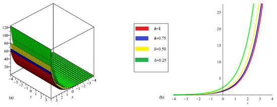
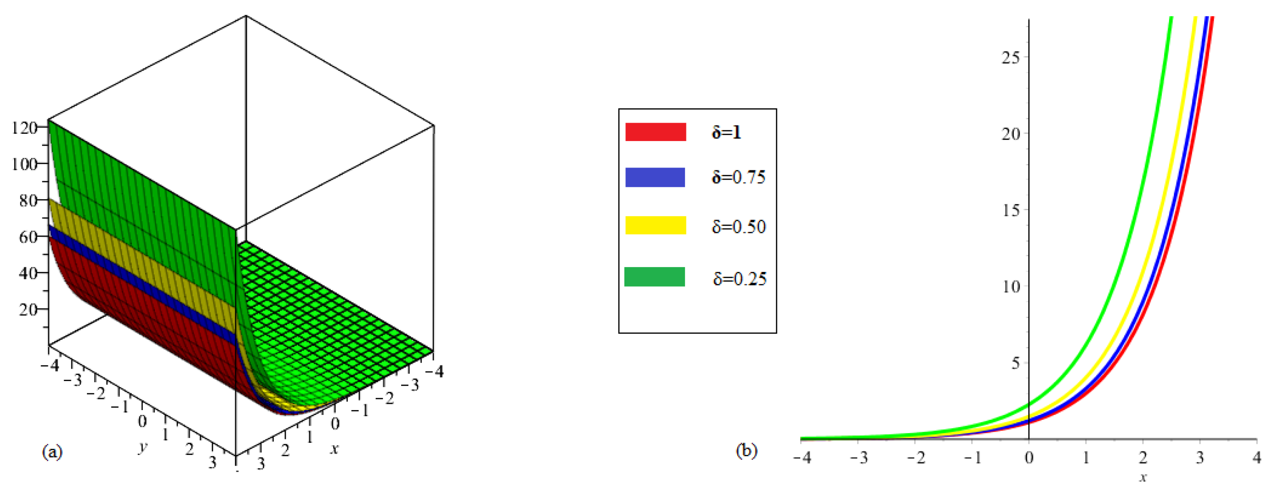
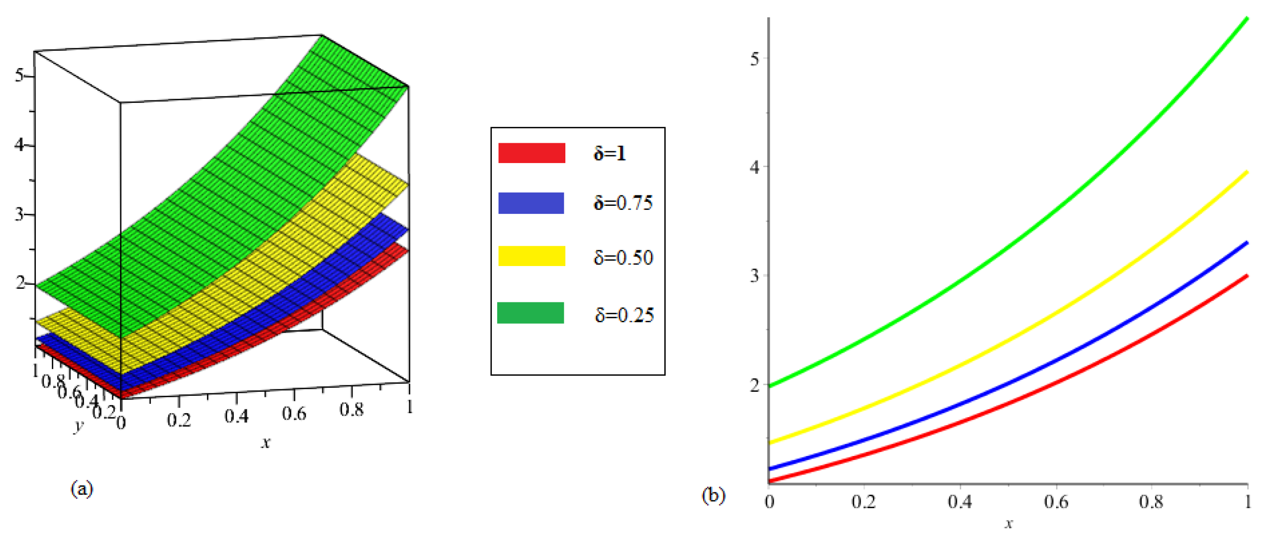
The Figure 1 shows the ETDM graph for Example 1 at various fractional order.

Figure 1. (a). the solution of ETDM at different fractional-order δ. (b). the graph show that the close relation with each other.

Example 2.

Consider the following linear time-fractional S-H equation

$$\frac{{\partial }^{\delta }\rho (\psi ,\tau )}{\partial {\tau }^{\delta }}+(1-b)\rho (\psi ,\tau )+2\frac{{\partial }^2\rho (\psi ,\tau )}{\partial {\psi }^2}+\frac{{\partial }^4\rho (\psi ,\tau )}{\partial {\psi }^4}=0,0<\delta \le 1$$

(35)

with initial condition

$$\rho (\psi ,0)=sin\left(\psi \right).$$

(36)

Taking Elzaki transformation of (35), we obtain

$$\begin{array}{cc}\hfill E\left\{\frac{{\partial }^{\delta }\rho }{\partial {\tau }^{\delta }}\right\}& =E\left[-(1-b)\rho (\psi ,\tau )-2\frac{{\partial }^2\rho (\psi ,\tau )}{\partial {\psi }^2}-\frac{{\partial }^4\rho (\psi ,\tau )}{\partial {\psi }^4}\right],\hfill \\ \hfill \frac{1}{s^{\delta }}E\left\{\rho (\psi ,\tau )\right\}-s^{2-\delta }\rho (\psi ,0)& =E\left[-(1-b)\rho (\psi ,\tau )-2\frac{{\partial }^2\rho (\psi ,\tau )}{\partial {\psi }^2}-\frac{{\partial }^4\rho (\psi ,\tau )}{\partial {\psi }^4}\right].\hfill \end{array}$$

The above algorithm’s simplified form is

$$E\left\{\rho (\psi ,\tau )\right\}=s^2\left\{\rho (\psi ,0)\right\}+s^{\delta }E\left[-(1-b)\rho (\psi ,\tau )-2\frac{{\partial }^2\rho (\psi ,\tau )}{\partial {\psi }^2}-\frac{{\partial }^4\rho (\psi ,\tau )}{\partial {\psi }^4}\right].$$

(37)

Using inverse Elzaki transformation, we get

$$\rho (\psi ,\tau )=\rho (\psi ,0)+E^{-}\left[s^{\delta }E\left[-(1-b)\rho (\psi ,\tau )-2\frac{{\partial }^2\rho (\psi ,\tau )}{\partial {\psi }^2}-\frac{{\partial }^4\rho (\psi ,\tau )}{\partial {\psi }^4}\right]\right].$$

(38)

Assume that the unknown $\rho (\psi ,\tau )$ function, in infinite series form, has the following solution

$$\begin{array}{cc}\hfill \rho (\psi ,\tau )& =\sum _{m=0}^{\infty }{\rho }_m(\psi ,\tau ),\hfill \\ \hfill \sum _{m=0}^{\infty }{\rho }_m(\psi ,\tau )& =sin\left(\psi \right)+E^{-}\left[s^{\delta }E\left[-(1-b)\rho (\psi ,\tau )-2\frac{{\partial }^2\rho (\psi ,\tau )}{\partial {\psi }^2}-\frac{{\partial }^4\rho (\psi ,\tau )}{\partial {\psi }^4}\right]\right].\hfill \end{array}$$

(39)

Here we will discuss the following two cases.

Case 1: ($b=0$). According to (35), we have

$${\rho }_0(\psi ,\tau )=sin\left(\psi \right);$$

for $m=0,$

$${\rho }_1(\psi ,\tau )=0;$$

for $m=1,$

$${\rho }_2(\psi ,\tau )=0;$$

for $m=n,$

$${\rho }_n(\psi ,\tau )=0.$$

Hence the solution to (35) in this case is

$$\rho (\psi ,\tau )=sin\left(\psi \right).$$

Case 2: $(b\ne 0)$. According to (37), we have

$${\rho }_0(\psi ,\tau )=sin\left(\psi \right);$$

for $m=0,$

$${\rho }_1(\psi ,\tau )=((b-1)+1)sin\left(\psi \right)\frac{1}{\Gamma (\delta +1)}{\tau }^{\delta };$$

for $m=1,$

$${\rho }_2(\psi ,\tau )=({(b-1)}^2+(b-1)+1)sin\left(\psi \right)\frac{1}{\Gamma (2\delta +1)}{\tau }^{2\delta };$$

for $m=2,$

$${\rho }_3(\psi ,\tau )=({(b-1)}^3+{(b-1)}^2+(b-1)+1)sin\left(\psi \right)\frac{1}{\Gamma (3\delta +1)}{\tau }^{3\delta };$$

for $m=3,$

$${\rho }_4(\psi ,\tau )=({(b-1)}^4+{(b-1)}^3+{(b-1)}^2+(b-1)+1)sin\left(\psi \right)\frac{1}{\Gamma (4\delta +1)}{\tau }^{4\delta }.$$

Similarly, the remaining ETDM solution elements ${\rho }_m$$(m\ge 3)$ are easy to get. Thus, we define the sequence of alternatives as

$$\begin{array}{cc}\hfill \rho (\psi ,\tau )& =\sum _{m=0}^{\infty }{\rho }_m(\psi ,\tau )={\rho }_0(\psi ,\tau )+{\rho }_1(\psi ,\tau )+{\rho }_2(\psi ,\tau )+{\rho }_3(\psi ,\tau )+{\rho }_4(\psi ,\tau )+\cdots ,\hfill \\ \hfill \rho (\psi ,\tau )& =sin\left(\psi \right)+((b-1)+1)sin\left(\psi \right)\frac{1}{\Gamma (\delta +1)}{\tau }^{\delta }\hfill \\ \hfill & +\left({(b-1)}^2+(b-1)+1\right)sin\left(\psi \right)\frac{1}{\Gamma (2\delta +1)}{\tau }^{2\delta }\hfill \\ \hfill & +\left({(b-1)}^3+{(b-1)}^2+(b-1)+1\right)sin\left(\psi \right)\frac{1}{\Gamma (3\delta +1)}{\tau }^{3\delta }\hfill \\ \hfill & +\left({(b-1)}^4+{(b-1)}^3+{(b-1)}^2+(b-1)+1\right)sin\left(\psi \right)\frac{1}{\Gamma (4\delta +1)}{\tau }^{4\delta }+\cdots .\hfill \end{array}$$

Exact solution for (33) at $\delta =1$ is

$$\rho (\psi ,\tau )=-\frac{1}{b}sin\left(\psi \right)\underset{N\to \infty }{lim}\sum _{n=0}^N\left(1-{(b-1)}^{n+1}\right)\frac{1}{\Gamma (n\delta +1)}{\tau }^{n\delta }.$$

(40)

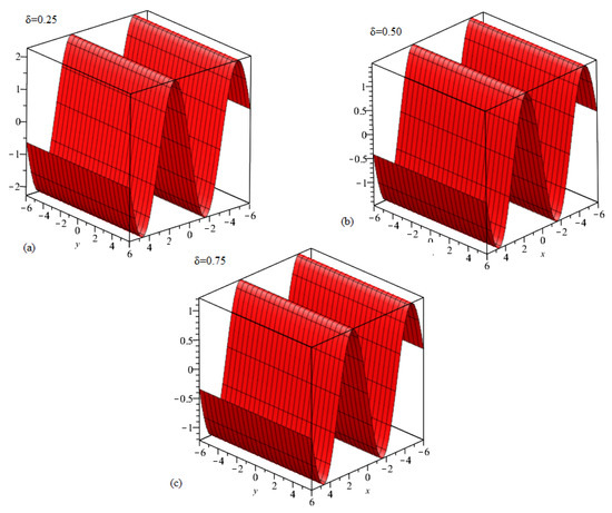
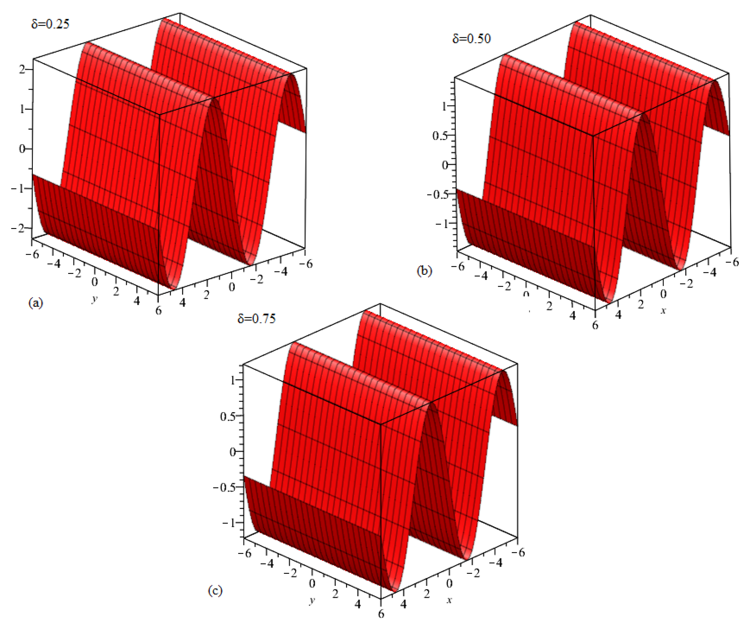
The Figure 2 shows ETDM solution graph at different fractional order for Example 2.

Figure 2. (a). δ = 0.25. (b). δ = 0.50. (c). δ = 0.75.

Example 3.

Consider the following linear time-fractional S-H equation

$$\frac{{\partial }^{\delta }\rho (\psi ,\tau )}{\partial {\tau }^{\delta }}+(1-b)\rho (\psi ,\tau )+2\frac{{\partial }^2\rho (\psi ,\tau )}{\partial {\psi }^2}+\frac{{\partial }^4\rho (\psi ,\tau )}{\partial {\psi }^4}=0,0<\delta \le 1$$

(41)

with initial condition

$$\rho (\psi ,0)=cos\left(\psi \right).$$

(42)

Taking Elzaki transformation of (41), we obtain

$$\begin{array}{cc}\hfill E\left\{\frac{{\partial }^{\delta }\rho }{\partial {\tau }^{\delta }}\right\}& =E\left[-(1-b)\rho (\psi ,\tau )-2\frac{{\partial }^2\rho (\psi ,\tau )}{\partial {\psi }^2}-\frac{{\partial }^4\rho (\psi ,\tau )}{\partial {\psi }^4}\right],\hfill \\ \hfill \frac{1}{s^{\delta }}E\left\{\rho (\psi ,\tau )\right\}-s^{2-\delta }\rho (\psi ,0)& =E\left[-(1-b)\rho (\psi ,\tau )-2\frac{{\partial }^2\rho (\psi ,\tau )}{\partial {\psi }^2}-\frac{{\partial }^4\rho (\psi ,\tau )}{\partial {\psi }^4}\right].\hfill \end{array}$$

The above algorithm’s simplified form is

$$E\left\{\rho (\psi ,\tau )\right\}=s^2\left\{\rho (\psi ,0)\right\}+s^{\delta }E\left[-(1-b)\rho (\psi ,\tau )-2\frac{{\partial }^2\rho (\psi ,\tau )}{\partial {\psi }^2}-\frac{{\partial }^4\rho (\psi ,\tau )}{\partial {\psi }^4}\right].$$

(43)

Using inverse Elzaki transformation, we get

$$\rho (\psi ,\tau )=\rho (\psi ,0)+E^{-}\left[s^{\delta }E\left[-(1-b)\rho (\psi ,\tau )-2\frac{{\partial }^2\rho (\psi ,\tau )}{\partial {\psi }^2}-\frac{{\partial }^4\rho (\psi ,\tau )}{\partial {\psi }^4}\right]\right].$$

(44)

Assume that the unknown $\rho (\psi ,\tau )$ function, in infinite series form, has the following solution

$$\begin{array}{cc}\hfill \rho (\psi ,\tau )& =\sum _{m=0}^{\infty }{\rho }_m(\psi ,\tau ),\hfill \\ \hfill \sum _{m=0}^{\infty }{\rho }_m(\psi ,\tau )& =cos\left(\psi \right)+E^{-}\left[s^{\delta }E\left[-(1-b)\rho (\psi ,\tau )-2\frac{{\partial }^2\rho (\psi ,\tau )}{\partial {\psi }^2}-\frac{{\partial }^4\rho (\psi ,\tau )}{\partial {\psi }^4}\right]\right].\hfill \end{array}$$

(45)

Here we will discuss the following two cases.

Case 1: ($b=0$). According to Equation (44), we have

$${\rho }_0(\psi ,\tau )=cos\left(\psi \right);$$

for $m=0,$

$${\rho }_1(\psi ,\tau )=0;$$

for $m=1,$

$${\rho }_2(\psi ,\tau )=0;$$

for $m=n,$

$${\rho }_n(\psi ,\tau )=0.$$

Hence the solution to (39) in this case is

$$\rho (\psi ,\tau )=cos\left(\psi \right).$$

Case 1: $(b\ne 0)$. According to (43), we have

$${\rho }_0(\psi ,\tau )=cos\left(\psi \right);$$

for $m=0,$

$${\rho }_1(\psi ,\tau )=((b-1)+1)cos\left(\psi \right)\frac{1}{\Gamma (\delta +1)}{\tau }^{\delta };$$

for $m=1,$

$${\rho }_2(\psi ,\tau )=({(b-1)}^2+(b-1)+1)cos\left(\psi \right)\frac{1}{\Gamma (2\delta +1)}{\tau }^{2\delta };$$

for $m=2,$

$${\rho }_3(\psi ,\tau )=({(b-1)}^3+{(b-1)}^2+(b-1)+1)cos\left(\psi \right)\frac{1}{\Gamma (3\delta +1)}{\tau }^{3\delta };$$

for $m=3,$

$${\rho }_4(\psi ,\tau )=({(b-1)}^4+{(b-1)}^3+{(b-1)}^2+(b-1)+1)cos\left(\psi \right)\frac{1}{\Gamma (4\delta +1)}{\tau }^{4\delta }.$$

Similarly, the remaining ETDM solution elements ${\rho }_m$$(m\ge 3)$ are easy to get. Thus, we define the sequence of alternatives as

$$\begin{array}{cc}\hfill \rho (\psi ,\tau )& =\sum _{m=0}^{\infty }{\rho }_m(\psi ,\tau )={\rho }_0(\psi ,\tau )+{\rho }_1(\psi ,\tau )+{\rho }_2(\psi ,\tau )+{\rho }_3(\psi ,\tau )+{\rho }_4(\psi ,\tau )+\cdots ,\hfill \\ \hfill \rho (\psi ,\tau )& =cos\left(\psi \right)+\left((b-1)+1\right)cos\left(\psi \right)\frac{1}{\Gamma (\delta +1)}{\tau }^{\delta }\hfill \\ \hfill & +\left({(b-1)}^2+(b-1)+1\right)cos\left(\psi \right)\frac{1}{\Gamma (2\delta +1)}{\tau }^{2\delta }\hfill \\ \hfill & +\left({(b-1)}^3+{(b-1)}^2+(b-1)+1\right)cos\left(\psi \right)\frac{1}{\Gamma (3\delta +1)}{\tau }^{3\delta }\hfill \\ \hfill & +\left({(b-1)}^4+{(b-1)}^3+{(b-1)}^2+(b-1)+1\right)cos\left(\psi \right)\frac{1}{\Gamma (4\delta +1)}{\tau }^{4\delta }+\cdots .\hfill \end{array}$$

Exact solution for (41) at $\delta =1$ is

$$\rho (\psi ,\tau )=-\frac{1}{b}cos\left(\psi \right)\underset{N\to \infty }{lim}\sum _{n=0}^N\left(1-{(b-1)}^{n+1}\right)\frac{1}{\Gamma (n\delta +1)}{\tau }^{n\delta }.$$

(46)

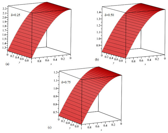
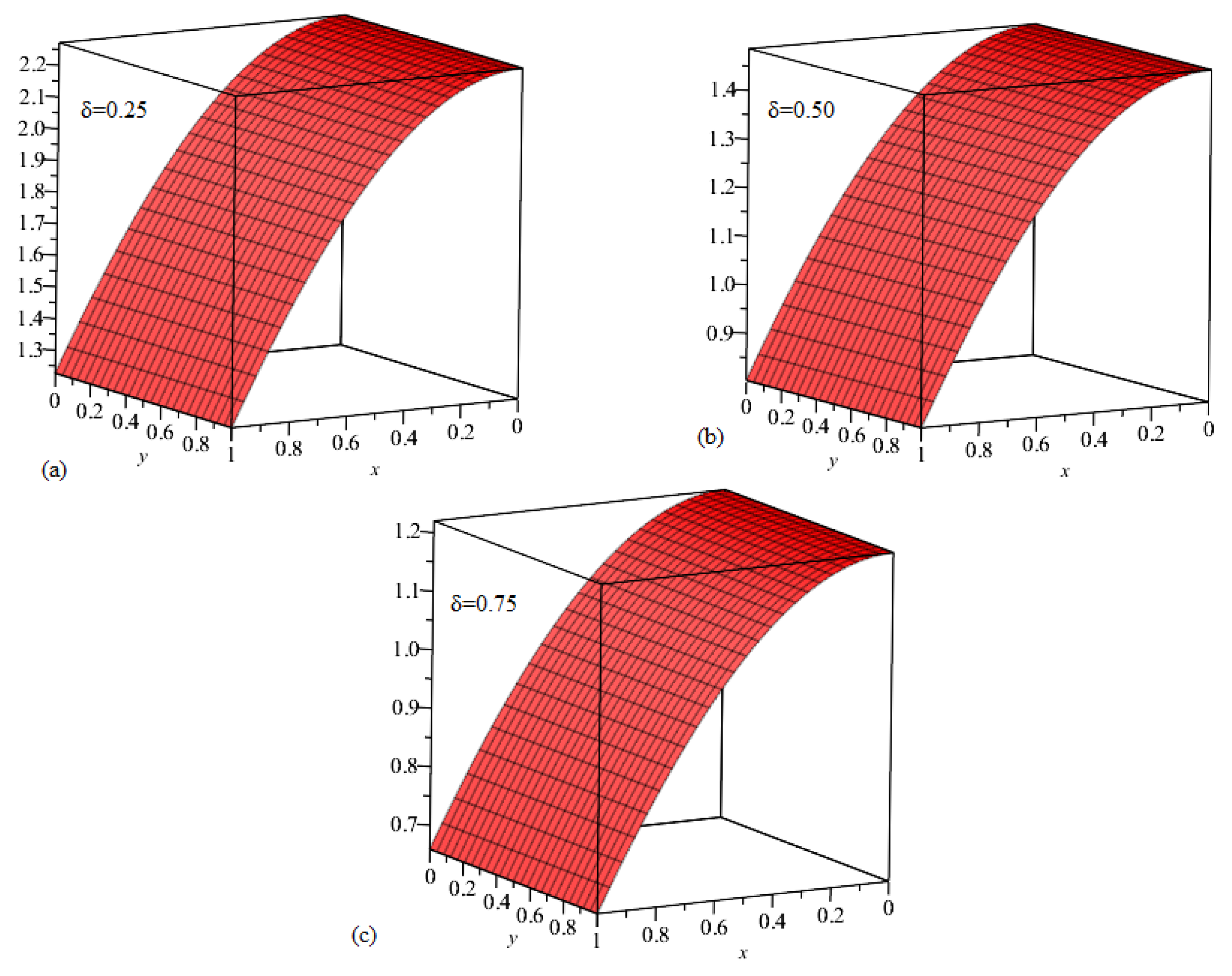
The Figure 3 shows ETDM solution graph at different fractional order for Example 3.

Figure 3. (a). δ = 0.25. (b). δ = 0.50. (c). δ = 0.75.

Example 4.

Consider the following linear time-fractional S-H equation

$$\frac{{\partial }^{\delta }\rho (\psi ,\tau )}{\partial {\tau }^{\delta }}+(1-b)\rho (\psi ,\tau )+2\frac{{\partial }^2\rho (\psi ,\tau )}{\partial {\psi }^2}-\sigma \frac{{\partial }^3\rho (\psi ,\tau )}{\partial {\psi }^3}+\frac{{\partial }^4\rho (\psi ,\tau )}{\partial {\psi }^4}=0,0<\delta \le 1$$

(47)

with initial condition

$$\rho (\psi ,0)=exp\left(\psi \right).$$

(48)

Taking Elzaki transformation of (47), we obtain

$$\begin{array}{cc}\hfill E\left\{\frac{{\partial }^{\delta }\rho }{\partial {\tau }^{\delta }}\right\}& =E\left[-(1-b)\rho (\psi ,\tau )-2\frac{{\partial }^2\rho (\psi ,\tau )}{\partial {\psi }^2}+\sigma \frac{{\partial }^3\rho (\psi ,\tau )}{\partial {\psi }^3}-\frac{{\partial }^4\rho (\psi ,\tau )}{\partial {\psi }^4}\right],\hfill \\ \hfill \frac{1}{s^{\delta }}E\left\{\rho (\psi ,\tau )\right\}-s^{2-\delta }\rho (\psi ,0)& =E\left[-(1-b)\rho (\psi ,\tau )-2\frac{{\partial }^2\rho (\psi ,\tau )}{\partial {\psi }^2}+\sigma \frac{{\partial }^3\rho (\psi ,\tau )}{\partial {\psi }^3}-\frac{{\partial }^4\rho (\psi ,\tau )}{\partial {\psi }^4}\right].\hfill \end{array}$$

The above algorithm’s simplified form is

$$E\left\{\rho (\psi ,\tau )\right\}=s^2\left\{\rho (\psi ,0)\right\}+s^{\delta }E\left[-(1-b)\rho (\psi ,\tau )-2\frac{{\partial }^2\rho (\psi ,\tau )}{\partial {\psi }^2}+\sigma \frac{{\partial }^3\rho (\psi ,\tau )}{\partial {\psi }^3}-\frac{{\partial }^4\rho (\psi ,\tau )}{\partial {\psi }^4}\right].$$

(49)

Using inverse Elzaki transformation, we get

$$\rho (\psi ,\tau )=\rho (\psi ,0)+E^{-}\left[s^{\delta }E\left[-(1-b)\rho (\psi ,\tau )-2\frac{{\partial }^2\rho (\psi ,\tau )}{\partial {\psi }^2}+\sigma \frac{{\partial }^3\rho (\psi ,\tau )}{\partial {\psi }^3}-\frac{{\partial }^4\rho (\psi ,\tau )}{\partial {\psi }^4}\right]\right].$$

(50)

Assume that the unknown $\rho (\psi ,\tau )$ function, in infinite series form, has the following solution

$$\begin{array}{cc}\hfill \rho (\psi ,\tau )& =\sum _{m=0}^{\infty }{\rho }_m(\psi ,\tau ),\hfill \\ \hfill \sum _{m=0}^{\infty }{\rho }_m(\psi ,\tau )& =exp\left(\psi \right)+E^{-}\left[s^{\delta }E\left[-(1-b)\rho (\psi ,\tau )-2\frac{{\partial }^2\rho (\psi ,\tau )}{\partial {\psi }^2}+\sigma \frac{{\partial }^3\rho (\psi ,\tau )}{\partial {\psi }^3}-\frac{{\partial }^4\rho (\psi ,\tau )}{\partial {\psi }^4}\right]\right].\hfill \end{array}$$

(51)

Thus, by comparing both sides of (49), we have

$${\rho }_0(\psi ,\tau )=exp\left(\psi \right);$$

for $m=0,$

$${\rho }_1(\psi ,\tau )=(b-4+\sigma )exp\left(\psi \right)\frac{1}{\Gamma (\delta +1)}{\tau }^{\delta };$$

for $m=1,$

$${\rho }_2(\psi ,\tau )={(b-4+\sigma )}^{2}exp\left(\psi \right)\frac{1}{\Gamma (2\delta +1)}{\tau }^{2\delta };$$

for $m=2,$

$${\rho }_3(\psi ,\tau )={(b-4+\sigma )}^{3}exp\left(\psi \right)\frac{1}{\Gamma (3\delta +1)}{\tau }^{3\delta };$$

for $m=3,$

$${\rho }_4(\psi ,\tau )={(b-4+\sigma )}^{4}exp\left(\psi \right)\frac{1}{\Gamma (4\delta +1)}{\tau }^{4\delta }.$$

Similarly, the remaining ETDM solution elements ${\rho }_m$$(m\ge 3)$ are easy to get. Thus, we define the sequence of alternatives as

$$\begin{array}{cc}\hfill \rho (\psi ,\tau )& =\sum _{m=0}^{\infty }{\rho }_m(\psi ,\tau )={\rho }_0(\psi ,\tau )+{\rho }_1(\psi ,\tau )+{\rho }_2(\psi ,\tau )+{\rho }_3(\psi ,\tau )+{\rho }_4(\psi ,\tau )+\cdots ,\hfill \\ \hfill \rho (\psi ,\tau )& =exp\left(\psi \right)+(b-4+\sigma )exp\left(\psi \right)\frac{1}{\Gamma (\delta +1)}{\tau }^{\delta }+{(b-4+\sigma )}^{2}exp\left(\psi \right)\frac{1}{\Gamma (2\delta +1)}{\tau }^{2\delta }\hfill \\ \hfill & +{(b-4+\sigma )}^{3}exp\left(\psi \right)\frac{1}{\Gamma (3\delta +1)}{\tau }^{3\delta }+{(b-4+\sigma )}^{4}exp\left(\psi \right)\frac{1}{\Gamma (4\delta +1)}{\tau }^{4\delta }+\cdots .\hfill \end{array}$$

Exact solution for (47) at $\delta =1$ is

$$\rho (\psi ,\tau )=exp\left(\psi \right)E_{\delta }((b-4+\sigma ){\tau }^{\delta }).$$

(52)

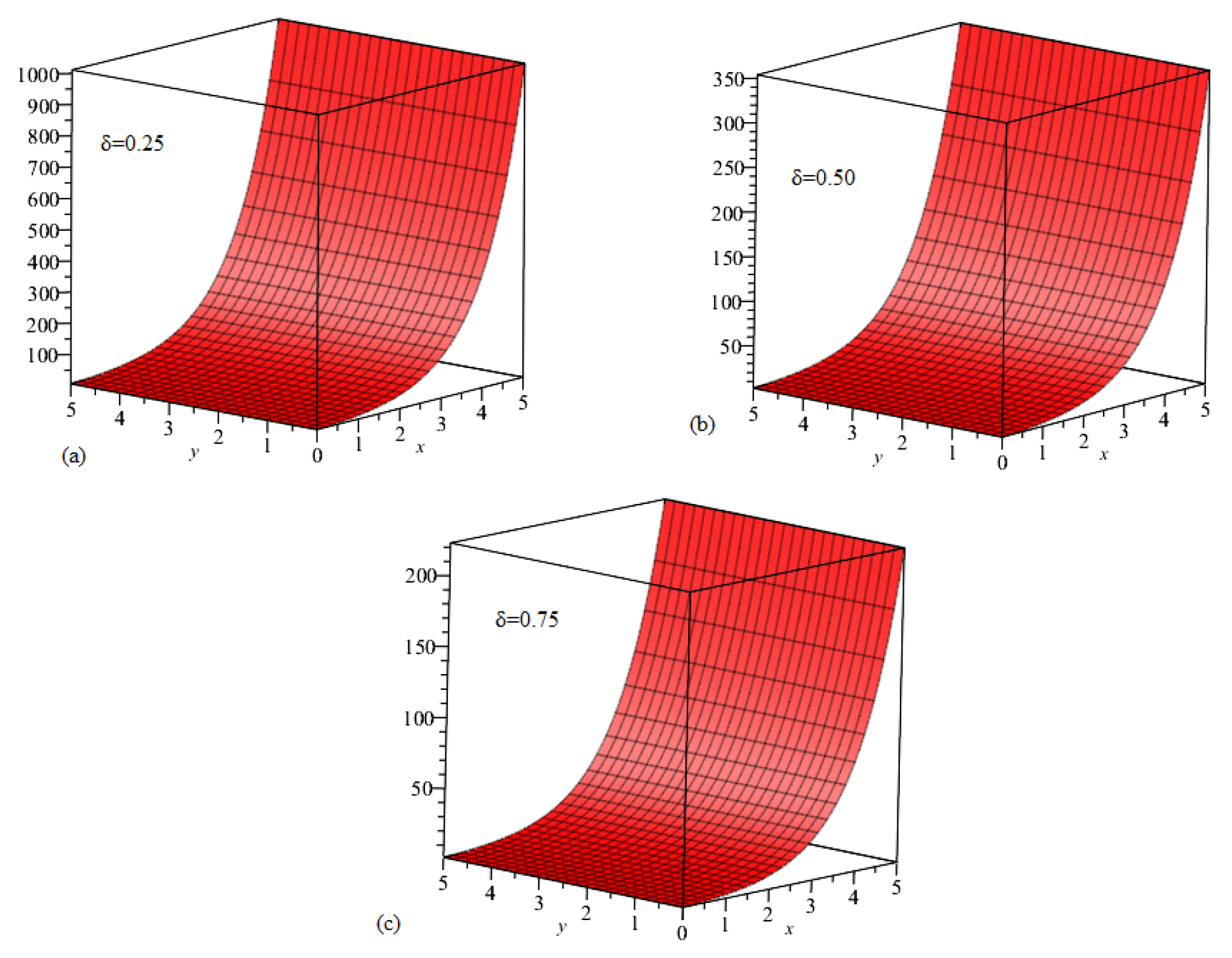
The Figure 4 shows ETDM solution graph at different fractional order for Example 4.

Figure 4. (a). δ = 0.25. (b). δ = 0.50. (c). δ = 0.75.

Example 5.

Consider the following non-linear time-fractional S-H equation

$$\frac{{\partial }^{\delta }\rho (\psi ,\tau )}{\partial {\tau }^{\delta }}+(1-b)\rho (\psi ,\tau )+2\frac{{\partial }^2\rho (\psi ,\tau )}{\partial {\psi }^2}+\frac{{\partial }^4\rho (\psi ,\tau )}{\partial {\psi }^4}-{\rho }^2(\psi ,\tau )+{\left(\frac{\partial \rho (\psi ,\tau )}{\partial \psi }\right)}^2=0,0<\delta \le 1,$$

(53)

with initial condition

$$\rho (\psi ,0)=exp\left(\psi \right).$$

(54)

Taking Elzaki transformation of (53), we obtain

$$\begin{array}{cc}\hfill E\left\{\frac{{\partial }^{\delta }\rho }{\partial {\tau }^{\delta }}\right\}& =E\left[-(1-b)\rho (\psi ,\tau )-2\frac{{\partial }^2\rho (\psi ,\tau )}{\partial {\psi }^2}-\frac{{\partial }^4\rho (\psi ,\tau )}{\partial {\psi }^4}+{\rho }^2(\psi ,\tau )-{\left(\frac{\partial \rho (\psi ,\tau )}{\partial \psi }\right)}^2\right],\hfill \\ \hfill \frac{1}{s^{\delta }}E\left\{\rho (\psi ,\tau )\right\}-s^{2-\delta }\rho (\psi ,0)& =E\left[-(1-b)\rho (\psi ,\tau )-2\frac{{\partial }^2\rho (\psi ,\tau )}{\partial {\psi }^2}-\frac{{\partial }^4\rho (\psi ,\tau )}{\partial {\psi }^4}+{\rho }^2(\psi ,\tau )-{\left(\frac{\partial \rho (\psi ,\tau )}{\partial \psi }\right)}^2\right].\hfill \end{array}$$

The above algorithm’s simplified form is

$$\begin{array}{cc}\hfill E\left\{\rho (\psi ,\tau )\right\}& =s^2\left\{\rho (\psi ,0)\right\}\hfill \\ \hfill & +s^{\delta }E\left[-(1-b)\rho (\psi ,\tau )-2\frac{{\partial }^2\rho (\psi ,\tau )}{\partial {\psi }^2}-\frac{{\partial }^4\rho (\psi ,\tau )}{\partial {\psi }^4}+{\rho }^2(\psi ,\tau )-{\left(\frac{\partial \rho (\psi ,\tau )}{\partial \psi }\right)}^2\right].\hfill \end{array}$$

(55)

Using inverse Elzaki transformation, we get

$$\begin{array}{cc}\hfill \rho (\psi ,\tau )& =\rho (\psi ,0)\hfill \\ \hfill & +E^{-}\left[s^{\delta }E\left[-(1-b)\rho (\psi ,\tau )-2\frac{{\partial }^2\rho (\psi ,\tau )}{\partial {\psi }^2}-\frac{{\partial }^4\rho (\psi ,\tau )}{\partial {\psi }^4}+{\rho }^2(\psi ,\tau )-{\left(\frac{\partial \rho (\psi ,\tau )}{\partial \psi }\right)}^2\right]\right].\hfill \end{array}$$

(56)

Assume that the unknown $\rho (\psi ,\tau )$ function, in infinite series form, has the following solution:

$$\rho (\psi ,\tau )=\sum _{m=0}^{\infty }{\rho }_m(\psi ,\tau ),$$

(57)

where the Adomian polynomials ${\rho }^2={\sum }_{m=0}^{\infty }{\mathcal{A}}_m$ and ${\left({\rho }_{\psi }\right)}^2={\sum }_{m=0}^{\infty }{\mathcal{B}}_m$ and the nonlinear terms have been characterised. (53) can be rewritten in the form using certain terms

$$\begin{array}{cc}\hfill \sum _{m=0}^{\infty }{\rho }_m(\psi ,\tau )& =\rho (\psi ,0)+E^{-}\left[s^{\delta }E\left[-(1-b)\rho (\psi ,\tau )-2\frac{{\partial }^2\rho (\psi ,\tau )}{\partial {\psi }^2}-\frac{{\partial }^4\rho (\psi ,\tau )}{\partial {\psi }^4}+\sum _{m=0}^{\infty }{\mathcal{A}}_m-\sum _{m=0}^{\infty }{\mathcal{B}}_m\right]\right],\hfill \\ \hfill \sum _{m=0}^{\infty }{\rho }_m(\psi ,\tau )& =exp\left(\psi \right)+E^{-}\left[s^{\delta }E\left[-(1-b)\rho (\psi ,\tau )-2\frac{{\partial }^2\rho (\psi ,\tau )}{\partial {\psi }^2}-\frac{{\partial }^4\rho (\psi ,\tau )}{\partial {\psi }^4}+\sum _{m=0}^{\infty }{\mathcal{A}}_m-\sum _{m=0}^{\infty }{\mathcal{B}}_m\right]\right].\hfill \end{array}$$

(58)

The decomposition of nonlinear terms by Adomian polynomials is defined as, according to (20),

$$\begin{array}{cc}\hfill & {\mathcal{A}}_0={\rho }_0^2,{\mathcal{A}}_1=2{\rho }_0{\rho }_1,\hfill \\ \hfill & {\mathcal{B}}_0={\left({\rho }_{0\psi }\right)}^2,{\mathcal{B}}_1=2{\rho }_{0\psi }{\rho }_{1\psi }.\hfill \end{array}$$

Thus, by comparing both sides of (56), we have

$${\rho }_0(\psi ,\tau )=exp\left(\psi \right);$$

for $m=0,$

$${\rho }_1(\psi ,\tau )=(b-4)exp\left(\psi \right)\frac{1}{\Gamma (\delta +1)}{\tau }^{\delta };$$

for $m=1,$

$${\rho }_2(\psi ,\tau )={(b-4)}^{2}exp\left(\psi \right)\frac{1}{\Gamma (2\delta +1)}{\tau }^{2\delta }.$$

Similarly, the remaining ETDM solution elements ${\rho }_m$$(m\ge 1)$ are easy to obtain. So, we define the sequence of alternatives as

$$\begin{array}{cc}\hfill \rho (\psi ,\tau )& =\sum _{m=0}^{\infty }{\rho }_m(\psi ,\tau )={\rho }_0(\psi ,\tau )+{\rho }_1(\psi ,\tau )+{\rho }_2(\psi ,\tau )+\cdots \hfill \\ \hfill \rho (\psi ,\tau )& =exp\left(\psi \right)+(b-4)exp\left(\psi \right)\frac{1}{\Gamma (\delta +1)}{\tau }^{\delta }+{(b-4)}^{2}exp\left(\psi \right)\frac{1}{\Gamma (2\delta +1)}{\tau }^{2\delta }+\cdots \hfill \end{array}$$

Exact solution for (51) at $\delta =1$ is

$$\rho (\psi ,\tau )=exp\left(\psi \right)E_{\delta }((b-4){\tau }^{\delta }).$$

(59)

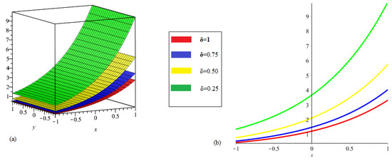
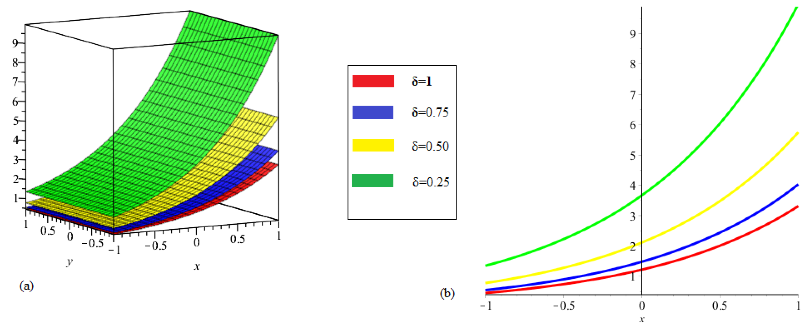
The Figure 5 shows the ETDM graph for Example 5 at various fractional order.

Figure 5. (a). the solution of ETDM at different fractional-order δ. (b). the graph show that the close relation with each other.

Example 6.

Consider the following non-linear time-fractional S-H equation

$$\begin{array}{cc}\hfill \frac{{\partial }^{\delta }\rho (\psi ,\tau )}{\partial {\tau }^{\delta }}& +(1-b)\rho (\psi ,\tau )+2\frac{{\partial }^2\rho (\psi ,\tau )}{\partial {\psi }^2}-\sigma \frac{{\partial }^3\rho (\psi ,\tau )}{\partial {\psi }^3}\hfill \\ \hfill & +\frac{{\partial }^4\rho (\psi ,\tau )}{\partial {\psi }^4}-{\rho }^2(\psi ,\tau )+{\left(\frac{\partial \rho (\psi ,\tau )}{\partial \psi }\right)}^2=0,0<\delta \le 1\hfill \end{array}$$

(60)

with initial condition

$$\rho (\psi ,0)=exp\left(\psi \right).$$

(61)

Taking Elzaki transformation of (59), we obtain

$$\begin{array}{cc}\hfill E\left\{\frac{{\partial }^{\delta }\rho }{\partial {\tau }^{\delta }}\right\}& =E\left[-(1-b)\rho (\psi ,\tau )-2\frac{{\partial }^2\rho (\psi ,\tau )}{\partial {\psi }^2}+\sigma \frac{{\partial }^3\rho (\psi ,\tau )}{\partial {\psi }^3}-\frac{{\partial }^4\rho (\psi ,\tau )}{\partial {\psi }^4}\right.\hfill \\ \hfill & \left.+{\rho }^2(\psi ,\tau )-{\left(\frac{\partial \rho (\psi ,\tau )}{\partial \psi }\right)}^2\right],\hfill \\ \hfill \frac{1}{s^{\delta }}E\left\{\rho (\psi ,\tau )\right\}-s^{2-\delta }\rho (\psi ,0)& =E\left[-(1-b)\rho (\psi ,\tau )-2\frac{{\partial }^2\rho (\psi ,\tau )}{\partial {\psi }^2}+\sigma \frac{{\partial }^3\rho (\psi ,\tau )}{\partial {\psi }^3}-\frac{{\partial }^4\rho (\psi ,\tau )}{\partial {\psi }^4}\right.\hfill \\ \hfill & \left.+{\rho }^2(\psi ,\tau )-{\left(\frac{\partial \rho (\psi ,\tau )}{\partial \psi }\right)}^2\right].\hfill \end{array}$$

The above algorithm’s simplified form is

$$\begin{array}{cc}\hfill E\left\{\rho (\psi ,\tau )\right\}& =s^2\left\{\rho (\psi ,0)\right\}+s^{\delta }E\left[-(1-b)\rho (\psi ,\tau )-2\frac{{\partial }^2\rho (\psi ,\tau )}{\partial {\psi }^2}+\sigma \frac{{\partial }^3\rho (\psi ,\tau )}{\partial {\psi }^3}-\frac{{\partial }^4\rho (\psi ,\tau )}{\partial {\psi }^4}\right.\hfill \\ \hfill & \left.+{\rho }^2(\psi ,\tau )-{\left(\frac{\partial \rho (\psi ,\tau )}{\partial \psi }\right)}^2\right].\hfill \end{array}$$

(62)

Using inverse Elzaki transformation, we get

$$\begin{array}{cc}\hfill \rho (\psi ,\tau )& =\rho (\psi ,0)+E^{-}\left[s^{\delta }E\left[-(1-b)\rho (\psi ,\tau )-2\frac{{\partial }^2\rho (\psi ,\tau )}{\partial {\psi }^2}+\sigma \frac{{\partial }^3\rho (\psi ,\tau )}{\partial {\psi }^3}+{\rho }^2(\psi ,\tau )\right.\right.\hfill \\ \hfill & \left.\left.-{\left(\frac{\partial \rho (\psi ,\tau )}{\partial \psi }\right)}^2\right]\right].\hfill \end{array}$$

(63)

Assume that the unknown $\rho (\psi ,\tau )$ function, in infinite series form, has the following solution

$$\rho (\psi ,\tau )=\sum _{m=0}^{\infty }{\rho }_m(\psi ,\tau ),$$

(64)

where the Adomian polynomials ${\rho }^2={\sum }_{m=0}^{\infty }{\mathcal{A}}_m$ and ${\left({\rho }_{\psi }\right)}^2={\sum }_{m=0}^{\infty }{\mathcal{B}}_m$ and the nonlinear terms have been characterised. (61) can be rewritten in the form using certain terms

$$\begin{array}{cc}\hfill \sum _{m=0}^{\infty }{\rho }_m(\psi ,\tau )=& \rho (\psi ,0)+E^{-}\left[s^{\delta }E\left[-(1-b)\rho (\psi ,\tau )-2\frac{{\partial }^2\rho (\psi ,\tau )}{\partial {\psi }^2}+\sigma \frac{{\partial }^3\rho (\psi ,\tau )}{\partial {\psi }^3}\right.\right.\hfill \\ \hfill & \left.\left.-\frac{{\partial }^4\rho (\psi ,\tau )}{\partial {\psi }^4}+\sum _{m=0}^{\infty }{\mathcal{A}}_m-\sum _{m=0}^{\infty }{\mathcal{B}}_m\right]\right],\hfill \\ \hfill \sum _{m=0}^{\infty }{\rho }_m(\psi ,\tau )=& exp\left(\psi \right)+E^{-}\left[s^{\delta }E\left[-(1-b)\rho (\psi ,\tau )-2\frac{{\partial }^2\rho (\psi ,\tau )}{\partial {\psi }^2}+\sigma \frac{{\partial }^3\rho (\psi ,\tau )}{\partial {\psi }^3}\right.\right.\hfill \\ \hfill & \left.\left.-\frac{{\partial }^4\rho (\psi ,\tau )}{\partial {\psi }^4}+\sum _{m=0}^{\infty }{\mathcal{A}}_m-\sum _{m=0}^{\infty }{\mathcal{B}}_m\right]\right].\hfill \end{array}$$

(65)

The decomposition of nonlinear terms by Adomian polynomials is defined as, according to (20),

$$\begin{array}{cc}\hfill & {\mathcal{A}}_0={\rho }_0^2,{\mathcal{A}}_1=2{\rho }_0{\rho }_1,\hfill \\ \hfill & {\mathcal{B}}_0={\left({\rho }_{0\psi }\right)}^2,{\mathcal{B}}_1=2{\rho }_{0\psi }{\rho }_{1\psi }.\hfill \end{array}$$

Thus, by comparing both sides of (63), we have

$${\rho }_0(\psi ,\tau )=exp\left(\psi \right);$$

for $m=0,$

$${\rho }_1(\psi ,\tau )=(b-4+\sigma )exp\left(\psi \right)\frac{1}{\Gamma (\delta +1)}{\tau }^{\delta };$$

for $m=1,$

$${\rho }_2(\psi ,\tau )={(b-4+\sigma )}^{2}exp\left(\psi \right)\frac{1}{\Gamma (2\delta +1)}{\tau }^{2\delta }.$$

Similarly, the remaining ETDM solution elements ${\rho }_m$$(m\ge 1)$ are easy to get. Thus, we define the sequence of alternatives as

$$\begin{array}{cc}\hfill \rho (\psi ,\tau )& =\sum _{m=0}^{\infty }{\rho }_m(\psi ,\tau )={\rho }_0(\psi ,\tau )+{\rho }_1(\psi ,\tau )+{\rho }_2(\psi ,\tau )+\cdots ,\hfill \\ \hfill \rho (\psi ,\tau )& =exp\left(\psi \right)+(b-4+\sigma )exp\left(\psi \right)\frac{1}{\Gamma (\delta +1)}{\tau }^{\delta }+{(b-4+\sigma )}^{2}exp\left(\psi \right)\frac{1}{\Gamma (2\delta +1)}{\tau }^{2\delta }+\cdots .\hfill \end{array}$$

Exact solution for (58) at $\delta =1$ is

$$\rho (\psi ,\tau )=exp\left(\psi \right)E_{\delta }((b-4+\sigma ){\tau }^{\delta }).$$

(66)

The Figure 6 shows the ETDM graph for Example 6 at various fractional order.

Figure 6. (a). the solution of ETDM at different fractional-order δ (b). the graph show that the close relation with each other.

6. Results and Discussion

In this paper, ETDM is implemented to solve time-fractional Swift–Hohenberg equations. The results, we get by using suggested technique are explain with the help of its graphical representation. Figure 1 show the 3D and 2D graph at different values of $\delta$. The ETDM solution graph are plotted at $b=5$ in the domain $-4\le \psi \le 4$. In Figure 2, ETDM solutions graphs at $\left(a\right)\delta =0.25$, $\left(b\right)\delta =0.50$ and $\left(a\right)\delta =0.75$ are plotted in which we fix $b=1$ in the given domain $-6\le \psi \le 6$. In Figure 3, the ETDM solutions at fractional orders are drawn. The graph (a) represent the solution of Example 3 at $\left(a\right)\delta =0.25$, $\left(b\right)\delta =0.50$, while graph (c) is the plotted at $\delta =0.75$. The given figures are plotted at $b=1$ with $\psi$ ranges from 0 to 1. In Figure 4, the ETDM solutions are plotted at various fractional order for $b=5,\sigma =1$ with $0\le \psi \le 5$. The graph (a) represent the solution of Example 4 at $\left(a\right)\delta =0.25$, $\left(b\right)\delta =0.50$, while graph (c) is the plotted at $\delta =0.75$. The solution in Figure 5 are calculated at different fractional-orders. It is observed that the solutions at various fractional-orders are converges to he solution of integer-order solution as fractional-orders approaches to an integer-order. The graphs are plotted at $b=5$ having $0\le \psi \le 1$. In Figure 6, the same graphical representation have been made at $b=5,\sigma =1$ and $-1\le \psi \le 1$.

7. Conclusions

An efficient analytical technique is used to solve time-fractional Swift–Hohenberg equations. We take the linear and nonlinear Swift–Hohenberg equations with different initial conditions to illustrate the effectiveness of such a method. The results we get are displayed by solution graph for each problem. The present method has simple, accurate, and straightforward implementation to solve fractional-order Swift–Hohenberg equations. In conclusion, the suggested approach is considered a sophisticated tool for the solution of other fractional-order differential equations.

References

- Baleanu, D.; Guvenc, Z.B.; Machado, J.T. New Trends in Nanotechnology and Fractional Calculus Applications; Springer: New York, NY, USA, 2010. [Google Scholar]
- Baleanu, D.; Machado, J.A.; Luo, A.C. Fractional Dynamics and Control; Springer Science & Business Media: New York, NY, USA, 2011. [Google Scholar]
- Liu, Q.; Xu, Y.; Kurths, J. Active vibration suppression of a novel airfoil model with fractional order viscoelastic constitutive relationship. J. Sound Vib. 2018, 432, 50–64. [Google Scholar] [CrossRef]
- Xu, Y.; Li, Y.; Liu, D. A method to stochastic dynamical systems with strong nonlinearity and fractional damping. Nonlinear Dyn. 2016, 83, 2311–2321. [Google Scholar] [CrossRef]
- Xu, Y.; Li, Y.; Liu, D.; Jia, W.; Huang, H. Responses of Duffing oscillator with fractional damping and random phase. Nonlinear Dyn. 2013, 74, 745–753. [Google Scholar] [CrossRef]
- Caputo, M. Linear models of dissipation whose Q is almost frequency independent II. Geophys. J. Int. 1967, 13, 529–539. [Google Scholar] [CrossRef]
- Ford, N.J.; Simpson, A.C. The numerical solution of fractional differential equations: Speed versus accuracy. Numer. Algorithms 2001, 26, 333–346. [Google Scholar] [CrossRef]
- Oldham, K.B.; Spanier, J. The Fractional Calculus; Academic Press: New York, NY, USA, 1974. [Google Scholar]
- Shah, N.A.; Dassios, I.; Chung, J.D. A decomposition method for a fractional-order multi-dimensional telegraph equation via the Elzaki transform. Symmetry 2021, 13, 8. [Google Scholar] [CrossRef]
- Ryzhkov, S.V.; Kuzenov, V.V. New realization method for calculating convective heat transfer near the hypersonic aircraft surface. Z. Angew. Math. Phys. 2019, 70, 1–9. [Google Scholar] [CrossRef]
- Saadeh, R.; Qazza, A.; Burqan, A. A new integral transform: ARA transform and its properties and applications. Symmetry 2020, 12, 925. [Google Scholar] [CrossRef]
- Caputo, M.; Fabrizio, M. A new definition of fractional derivative without singular kernel. Fract. Differ. Appl. 2015, 2, 731–785. [Google Scholar]
- Losada, J.; Nieto, J.J. Properties of the new fractional derivative without singular kernel. Fract. Differ. Appl. 2015, 2, 87–92. [Google Scholar]
- Sunthrayuth, P.; Zidan, A.M.; Yao, S.-W.; Shah, R.; Inc, M. The Comparative Study for Solving Fractional-Order Fornberg–Whitham Equation via ρ-Laplace Transform. Symmetry 2021, 5, 784. [Google Scholar] [CrossRef]
- Baleanu, D.; Mustafa, O.G. On the global existence of solutions to a class of fractional differential equations. Comput. Math. Appl. 2010, 59, 35–41. [Google Scholar] [CrossRef] [Green Version]
- Yousef, F.; Alquran, M.; Jaradat, I.; Momani, S.; Baleanu, D. Ternary-fractional differential transform schema: Theory and application. Adv. Differ. Equ. 2019, 2019, 197. [Google Scholar] [CrossRef]
- Bokhari, A.; Baleanu, D.; Belgacem, R. Application of Shehu transform to Atangana-Baleanu derivatives. Int. J. Math. Comput. Sci. 2019, 20, 101–107. [Google Scholar] [CrossRef] [Green Version]
- He, J.H.; Ji, F.Y. Two-scale mathematics and fractional calculus for thermodynamics. Therm. Sci. 2019, 21, 2131–2133. [Google Scholar] [CrossRef]
- Wang, K.L.; Yao, S.W.; Yang, H.W. A fractal derivative model for snow’s thermal insulation property. Therm. Sci. 2019, 23, 2351–2354. [Google Scholar] [CrossRef]
- Kakutani, T.; Ono, H. Weak non-linear hydromagnetic waves in a cold collision-free plasma. J. Phys. Soc. Japan 1969, 26, 1305–1318. [Google Scholar] [CrossRef]
- Yang, X.J.; Srivastava, H.M.; Machado, J.A. A new fractional derivative without singular kernel: Application to the modelling of the steady heat flow. Therm. Sci. 2016, 20, 753–756. [Google Scholar] [CrossRef]
- Yang, X.J. Fractional derivatives of constant and variable orders applied to anomalous relaxation models in heat-transfer problems. Therm. Sci. 2017, 21, 1161–1171. [Google Scholar] [CrossRef] [Green Version]
- Singh, J.; Kumar, D.; Kumar, S. A new fractional model of nonlinear shock wave equation arising in flow of gases. Nonlinear Eng. 2014, 3, 43–50. [Google Scholar] [CrossRef]
- Naeem, M.; Zidan, A.M.; Nonlaopon, K.; Syam, M.I.; Al-Zhour, Z.; Shah, R. A New Analysis of Fractional-Order Equal-Width Equations via Novel Techniques. Symmetry 2021, 5, 886. [Google Scholar] [CrossRef]
- Paolo, D.B.; Fattorusso, L.; Versaci, M. Electrostatic field in terms of geometric curvature in membrane MEMS devices. Commun. Appl. Ind. Math. 2017, 8, 165–184. [Google Scholar]
- Yong, L.; Wang, H.; Chen, X.; Yang, X.; You, Z.; Dong, S.; Gao, J. Shear property, high-temperature rheological performance and low-temperature flexibility of asphalt mastics modified with bio-oil. Constr. Build. Mater. 2018, 174, 30–37. [Google Scholar]
- Meerschaert, M.M.; Tadjeran, C. Finite difference approximations for two-sided space-fractional partial differential equations. Appl. Numer. Math. 2006, 56, 80–90. [Google Scholar] [CrossRef]
- Ray, S.S.; Bera, R.K. Analytical solution of the Bagley Torvik equation by Adomian decomposition method. Appl. Math. Comput. 2005, 168, 398–410. [Google Scholar] [CrossRef]
- Jiang, Y.; Ma, J. High-order finite element methods for time-fractional partial differential equations. J. Comput. Appl. Math. 2011, 235, 3285–3290. [Google Scholar] [CrossRef] [Green Version]
- Odibat, Z.; Momani, S.; Erturk, V.S. Generalized differential transform method: Application to differential equations of fractional order. Appl. Math. Comput. 2008, 197, 467–477. [Google Scholar] [CrossRef]
- Arikoglu, A.; Ozkol, I. Solution of fractional differential equations by using differential transform method. Chaos Solitons Fractals 2007, 34, 1473–1481. [Google Scholar] [CrossRef]
- Zhang, X.; Zhao, J.; Liu, J.; Tang, B. Homotopy perturbation method for two dimensional time-fractional wave equation. Appl. Math. Model. 2014, 38, 5545–5552. [Google Scholar] [CrossRef]
- Prakash, A. Analytical method for space-fractional telegraph equation by homotopy perturbation transform method. Nonlinear Eng. 2016, 5, 123–128. [Google Scholar] [CrossRef]
- Dhaigude, C.; Nikam, V. Solution of fractional partial differential equations using iterative method. Fract. Calc. Appl. Anal. 2012, 15, 684–699. [Google Scholar] [CrossRef]
- Safari, M.; Ganji, D.D.; Moslemi, M. Application of He’s variational iteration method and Adomian’s decomposition method to the fractional KdV-Burgers-Kuramoto equation. Comput. Math. Appl. 2009, 58, 2091–2097. [Google Scholar] [CrossRef] [Green Version]
- Liao, S.J. The Proposed Homotopy Analysis Technique for the Solution of Nonlinear Problems. Ph.D. Thesis, Shanghai Jiao Tong University, Shanghai, China, 1992. [Google Scholar]
- Liao, S. Homotopy analysis method: A new analytical technique for nonlinear problems. Commun. Nonlinear Sci. Numer. Simulat. 1997, 2, 95–100. [Google Scholar] [CrossRef]
- Liao, S. On the homotopy analysis method for nonlinear problems. Appl. Math. Comput. 2004, 147, 499–513. [Google Scholar] [CrossRef]
- Abbasbandy, S.; Hashemi, M.S.; Hashim, I. On convergence of homotopy analysis method and its application to fractional integro-differential equations. Quaest. Math. 2013, 36, 93–105. [Google Scholar] [CrossRef]
- Kumar, D.; Singh, J.; Baleanu, D. A fractional model of convective radial fins with temperature-dependent thermal conductivity. Rom. Rep. Phys. 2017, 69, 103. [Google Scholar]
- Kumar, D.; Agarwal, R.P.; Singh, J. A modified numerical scheme and convergence analysis for fractional model of Lienards equation. J. Comput. Appl. Math. 2018, 339, 405–413. [Google Scholar] [CrossRef]
- Hang, X.; Cang, J. Analysis of a time fractional wave-like equation with the homotopy analysis method. Phys. Lett. A 2008, 372, 1250–1255. [Google Scholar]
- Dehghan, M.; Manafian, J.; Saadatmandi, A. The solution of the linear fractional partial differential equations using the homotopy analysis method. Z. Nat. A 2010, 65, 935–949. [Google Scholar] [CrossRef] [Green Version]
- Goufo, E.F.D.; Pene, M.K.; Mwambakana, J.N. Duplication in a model of rock fracture with fractional derivative without singular kernel. Open Math. 2015, 13, 839–846. [Google Scholar] [CrossRef] [Green Version]
- Jafari, H.; Das, S.; Tajadodi, H. Solving a multi-order fractional differential equation using homotopy analysis method. J. King Saud Univ. Sci. 2011, 23, 151–155. [Google Scholar] [CrossRef] [Green Version]
- Diethelm, K.; Ford, N.J. Multi-order fractional differential equations and their numerical solution. Appl. Math. Comput. 2004, 154, 621–640. [Google Scholar] [CrossRef]
- Daftardar-Gejji, V.; Jafari, H. An iterative method for solving nonlinear functional equations. J. Math. Anal. Appl. 2006, 316, 753–763. [Google Scholar] [CrossRef] [Green Version]
Publisher’s Note: MDPI stays neutral with regard to jurisdictional claims in published maps and institutional affiliations. |
© 2021 by the authors. Licensee MDPI, Basel, Switzerland. This article is an open access article distributed under the terms and conditions of the Creative Commons Attribution (CC BY) license (https://creativecommons.org/licenses/by/4.0/).