Half Logistic Inverse Lomax Distribution with Applications

Abstract

The last years have revealed the importance of the inverse Lomax distribution in the understanding of lifetime heavy-tailed phenomena. However, the inverse Lomax modeling capabilities have certain limits that researchers aim to overcome. These limits include a certain stiffness in the modulation of the peak and tail properties of the related probability density function. In this paper, a solution is given by using the functionalities of the half logistic family. We introduce a new three-parameter extended inverse Lomax distribution called the half logistic inverse Lomax distribution. We highlight its superiority over the inverse Lomax distribution through various theoretical and practical approaches. The derived properties include the stochastic orders, quantiles, moments, incomplete moments, entropy (Rényi and q) and order statistics. Then, an emphasis is put on the corresponding parametric model. The parameters estimation is performed by six well-established methods. Numerical results are presented to compare the performance of the obtained estimates. Also, a simulation study on the estimation of the Rényi entropy is proposed. Finally, we consider three practical data sets, one containing environmental data, another dealing with engineering data and the last containing insurance data, to show how the practitioner can take advantage of the new half logistic inverse Lomax model.

1. Introduction

Over the last century, many significant distributions have been introduced to serve as models in applied sciences. Among them, the so-called generalized beta distribution introduced by [1] is at the top of the list in terms of usefulness. The main feature of the generalized beta distribution is to be very rich; It includes a plethora of named distributions (to our knowledge, over thirty). In this paper, we focus our attention on one of the most attractive of these distributions, known as the inverse Lomax (IL) distribution. Mathematically, it also corresponds to the distribution of $Y=X^{-1}$, where X is a random variable following the famous Lomax distribution (see [2]). Thus, the cumulative distribution function (cdf) of the IL distribution is given by

$$\begin{array}{c}\hfill G(x;\alpha ,\lambda )={\left(1+\frac{x^{-1}}{\lambda }\right)}^{-\alpha },x>0,\end{array}$$

(1)

where $\lambda$ is a positive scale parameter and $\alpha$ is a positive shape parameter, and $G(x;\alpha ,\lambda )=0$ for $x\le 0$. The reasons for the interest of the IL distribution are the following ones. It has proved itself as a statistical model in various applications, including economics and actuarial sciences (see [3]) and geophysics (see [4]). Also, the mathematical and inferential aspects of the IL distribution are well developed. See, for instance, Reference [5] for the Lorenz ordering of order statistics, Reference [6] for the parameters estimation in a Bayesian setting, Reference [7] for the parameters estimation from hybrid censored samples, Reference [8] for the study of the reliability estimator under type II censoring and Reference [9] for the Bayesian estimation of two-component mixture of the IL distribution under type I censoring. Despite an interesting compromise between simplicity and accuracy, the IL model suffers from a certain rigidity in the peak (punctual and roundness) and tail properties. This motivates the developments of diverse parametric extensions, such as the inverse power Lomax distribution introduced by [10], the Weibull IL distribution studied by [11] and the Marshall-Olkin IL distribution studied by [12].

In this paper, we introduce and discuss a new extension of the IL distribution based on the half logistic generated family of distributions studied by [13]. This general family is defined by the following cdf:

$$\begin{array}{c}\hfill F(x;\beta ,\xi )=\frac{1-{[1-G(x;\xi )]}^{\beta }}{1+{[1-G(x;\xi )]}^{\beta }},x\in \mathbb{R},\end{array}$$

(2)

where $\beta$ is a positive shape parameter and $G(x;\xi )$ denotes a cdf of a continuous univariate distribution. Here, $\xi$ represents a vector of parameter(s) related to the corresponding parental distribution. The main motivations behind the half logistic generated family are as follows. First, it is proved in [13] that the combined effect of the considered ratio and power transformations can significantly enrich the parental distribution, improving the flexibility of the mode, median, skewness and tail, with a positive impact on the analyses of practical data sets. The normal, Weibull and Fréchet distributions have been considered as parents in [13]. Recent studies have also pointed out these facts in other practical settings. See, for instance, References [14,15,16] which consider the generalized Weibull, Topp-Leone and power Lomax distributions as parental distributions, respectively. However, the half logistic generated family remains underexploited and, based on the previous promising studies, needs more thorough attention. In this paper, we contribute in this direction of work, with the consideration of the IL distribution as a parent.

Thus, we introduce a new attractive lifetime distribution with three parameters called the half logistic IL (HLIL) distribution. The cdf of the HLIL distribution with parameter vector $\mathbf{\varphi }=(\alpha ,\lambda ,\beta )$ is obtained by inserting (1) into (2) as

$$\begin{array}{c}\hfill F(x;\mathbf{\varphi })=\frac{1-{\left[1-{\left(1+\frac{x^{-1}}{\lambda }\right)}^{-\alpha }\right]}^{\beta }}{1+{\left[1-{\left(1+\frac{x^{-1}}{\lambda }\right)}^{-\alpha }\right]}^{\beta }},x>0,\end{array}$$

(3)

where $\lambda$ is a positive scale parameter, and $\alpha$ and $\beta$ are two positive shape parameters, and $F(x;\mathbf{\varphi })=0$ for $x\le 0$. With various theoretical and practical developments, we show how the functionalities of the half logistic generated family confer new application perspectives to the IL distribution. In particular, the preference of the HLIL distribution over the IL distribution is motivated by the following findings: (i) the decay rate of convergence of the probability density function (pdf) of the HLIL distribution can be modulated by adjusting $\beta$ contrary to the fixed one of the IL distribution, (ii) the mode of the HLIL distribution is positively affected by $\beta$ on the numerical point of view, (iii) the almost constant hazard rate shape is reachable for the HLIL distribution, this is not the case of the IL distribution, (iv) the skewness of the HLIL distribution is more flexible to the IL distribution, with the observation of an ‘almost symmetric shape’ for some parameter values, and (v) the kurtosis of the HLIL distribution varies between the mesokurtic and leptokurtic cases, with a specific ‘roundness shape property’ for some parameter values. Thus, from the modeling point of view, in the category of heavy right-tailed distributions, the HLIL distribution is very flexible on the peak and tails, and its pdf allows the ‘almost symmetric shape and/or round shape fitting’ of the histogram of the data, which is not possible with the IL distribution, for instance. In this study, after developing the mathematical features of the HLIL distribution, we emphasize its inferential aspects, which are of comparable complexity with those of the IL distribution. In particular, from the related HLIL model, we develop the parameters estimation by six various well-established methods. Also, a simulation study on the estimation of the Rényi entropy is proposed. Then, three applications in environment, engineering and insurance are given; Three data sets in these fields are analysed in the rules of the art, revealing the superiority of the HLIL model over some known competitors, including the reference IL model.

The remainder of this article is arranged as follows. The important functions related to the HLIL distribution are presented in Section 2. Section 3 investigates some properties of the HLIL distribution such as stochastic orders, moments, Rényi and q-entropies, and order statistics. Section 4 studies parameter estimates for the HLIL model based on six different methods, namely: maximum likelihood (ML), least squares (LS), weighted least squares (WLS), percentile (PC), Cramér-von Mises (CV) and maximum product of spacing (MPS) methods, with practical guarantees via a simulation study. Two real life data sets are presented and analyzed to show the benefit of the HLIL model compared with some other known models in Section 5. The article ends with some concluding remarks in Section 6.

2. Important Functions

This section is devoted to some important functions of the HLIL distribution, with applications.

2.1. The Probability Density Function

Upon differentiation of $F(x;\mathbf{\varphi })$ with respect to x, the pdf of the HLIL distribution is given by

$$\begin{array}{c}\hfill f(x;\mathbf{\varphi })=\frac{\frac{2\beta \alpha }{\lambda }{x}^{-2}{\left(1+\frac{x^{-1}}{\lambda }\right)}^{-\alpha -1}{\left[1-{\left(1+\frac{x^{-1}}{\lambda }\right)}^{-\alpha }\right]}^{\beta -1}}{{\left\{1+{\left[1-{\left(1+\frac{x^{-1}}{\lambda }\right)}^{-\alpha }\right]}^{\beta }\right\}}^2},x,\lambda ,\alpha ,\beta >0.\end{array}$$

(4)

An analytical study of this function is proposed below. First, the following equivalence holds. As $x\to 0$, we have $f(x;\mathbf{\varphi })\sim (\beta \alpha {\lambda }^{\alpha }/2)x^{\alpha -1}$, and, as $x\to +\infty$, we have $f(x;\mathbf{\varphi })\sim (2\beta {\alpha }^{\beta }/{\lambda }^{\beta })x^{-\beta -1}$. Thus, for $\alpha \in (0,1)$, we have ${lim}_{x\to 0}f(x;\mathbf{\varphi })=+\infty$, for $\alpha =1$, we have ${lim}_{x\to 0}f(x;\mathbf{\varphi })=\beta \lambda /2$ and for $\alpha >1$, we have ${lim}_{x\to 0}f(x;\mathbf{\varphi })=0$. Furthermore, without special constraints on the parameters, we have ${lim}_{x\to +\infty }f(x;\mathbf{\varphi })=0$ with a converge rate depending on the parameter $\beta$ making the difference with the former IL distribution. The obtained equivalence results are also crucial to determine the existence of moment measures and functions (raw moments, moment generating function, entropy…)

A change point of $f(x;\mathbf{\varphi })$, say $x_m$, satisfies $f^{\prime }(x_m;\mathbf{\varphi })=0$ or, equivalently, ${\{log\left[f(x_m;\mathbf{\varphi })\right]\}}^{\prime }=0$. After some developments, we arrive at the following equation:

$$\begin{array}{cc}\hfill & -\frac{2}{x_m}+(\alpha +1)\frac{1}{x_m(\lambda x_m+1)}-\frac{\alpha (\beta -1)}{\lambda }\frac{x_m^{-2}{\left(1+\frac{x_m^{-1}}{\lambda }\right)}^{-\alpha -1}}{1-{\left(1+\frac{x_m^{-1}}{\lambda }\right)}^{-\alpha }}\hfill \\ \hfill & +\frac{2\alpha \beta }{\lambda }\frac{x_m^{-2}{\left(1+\frac{x_m^{-1}}{\lambda }\right)}^{-\alpha -1}{\left[1-{\left(1+\frac{x_m^{-1}}{\lambda }\right)}^{-\alpha }\right]}^{\beta -1}}{1+{\left[1-{\left(1+\frac{x_m^{-1}}{\lambda }\right)}^{-\alpha }\right]}^{\beta }}=0.\hfill \end{array}$$

Clearly, from this equation, we can not derive an analytical formula for $x_m$. It is however clear that it is modulated by the parameter $\beta$, offering a certain flexibility in this regard. Also, the presence of several change points is not excluded. However, for a given $\mathbf{\varphi }$, it can be determined numerically by using any standard mathematical software, as Mathematica, Matlab or R.

From the theoretical point of view, the fine shape properties of $f(x;\mathbf{\varphi })$ are given by the study of the signs of the first and second order derivatives of $f(x;\mathbf{\varphi })$ with respect to x. However, the expressions obtained are very complex and do not make it possible to determine the exact range of values of the parameters characterizing the different shapes. This obstacle motivates a graphic study. 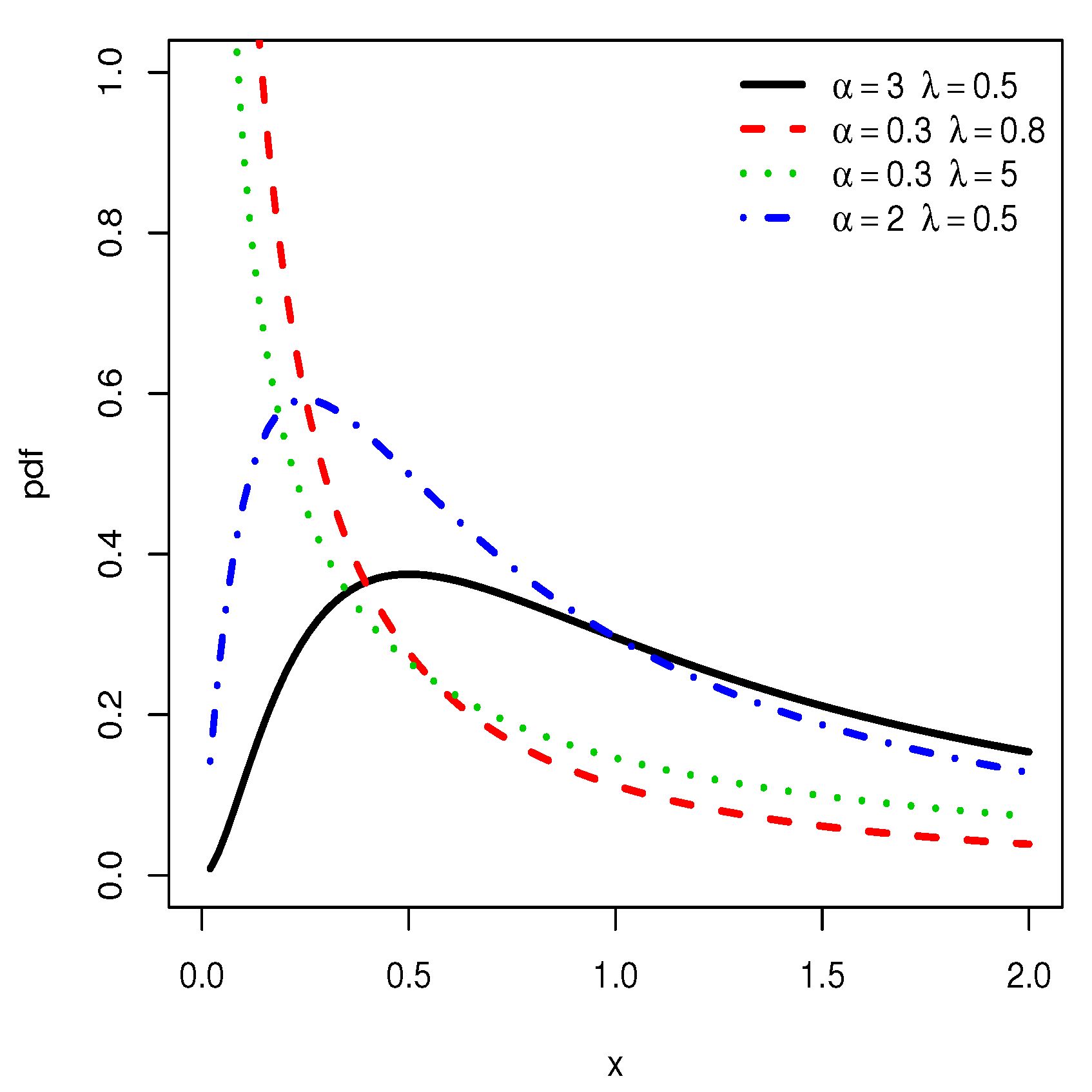Figure 1 displays some plots of $f(x;\mathbf{\varphi })$ for some different values of the parameters.

Figure 1. Plots of the pdf of the half logistic inverse Lomax (HLIL) distribution for various choices of $\alpha$, $\beta$ and $\lambda$.

From Figure 1, we notice that the pdf of the HLIL distribution can be reversed J, right-skewed and almost symmetrical shaped. Based on several empirical observations, we conjecture that the J shapes are mainly observed for $\alpha \in (0,1)$. The various forms of the curves also indicate a certain versatility in mode, skewness and kurtosis with is clearly a plus in terms of modeling; the pdf allows the ‘almost symmetric shape and/or round shape fitting’ of the histogram of heavy-tailed data. This specificity is not observed for the IL distribution, as attested by Figure 2.

Figure 2. Plots of the pdf of the IL distribution for various choices of $\alpha$ and $\lambda$.

2.2. Reliability Functions

Here, we present the main reliability functions of the HLIL distribution, which are of importance for various applications. The survival function (sf) and cumulative hazard rate function (chrf) of the HLIL distribution are, respectively, given by

$$\begin{array}{c}\hfill R(x;\mathbf{\varphi })=1-F(x;\mathbf{\varphi })=\frac{2{\left[1-{\left(1+\frac{x^{-1}}{\lambda }\right)}^{-\alpha }\right]}^{\beta }}{1+{\left[1-{\left(1+\frac{x^{-1}}{\lambda }\right)}^{-\alpha }\right]}^{\beta }},x>0,\end{array}$$

(5)

and $R(x;\mathbf{\varphi })=1$ for $x\le 0$, and

$$\begin{array}{cc}\hfill H(x;\mathbf{\varphi })& =-log\left[R(x;\mathbf{\varphi })\right]\hfill \\ \hfill & =-log\left(2\right)-\beta log\left[1-{\left(1+\frac{x^{-1}}{\lambda }\right)}^{-\alpha }\right]+log\left\{1+{\left[1-{\left(1+\frac{x^{-1}}{\lambda }\right)}^{-\alpha }\right]}^{\beta }\right\},\hfill \end{array}$$

and $H(x;\mathbf{\varphi })=0$ for $x\le 0$. Also, the hazard rate function (hrf) is obtained as

$$\begin{array}{cc}\hfill & h(x;\mathbf{\varphi })=\frac{f(x;\mathbf{\varphi })}{R(x;\mathbf{\varphi })}=\frac{\frac{\beta \alpha }{\lambda }{x}^{-2}{\left(1+\frac{x^{-1}}{\lambda }\right)}^{-\alpha -1}}{\left\{1+{\left[1-{\left(1+\frac{x^{-1}}{\lambda }\right)}^{-\alpha }\right]}^{\beta }\right\}\left[1-{\left(1+\frac{x^{-1}}{\lambda }\right)}^{-\alpha }\right]}\hfill \end{array}$$

and $h(x;\mathbf{\varphi })=0$ for $x\le 0$. The analytical study of this hrf is important to understand the modeling capacity of the HLIL model. First, the following equivalences are true. As $x\to 0$, we have $h(x;\mathbf{\varphi })\sim (\beta \alpha {\lambda }^{\alpha }/2)x^{\alpha -1}$ and, as $x\to +\infty$, we have $h(x;\mathbf{\varphi })\sim \beta x^{-1}$. We deduce the following asymptotic properties, which are similar to those for $f(x;\mathbf{\varphi })$. For $\alpha \in (0,1)$, we have ${lim}_{x\to 0}h(x;\mathbf{\varphi })=+\infty$, for $\alpha =1$, we have ${lim}_{x\to 0}h(x;\mathbf{\varphi })=\beta \lambda /2$ and for $\alpha >1$, we have ${lim}_{x\to 0}h(x;\mathbf{\varphi })=0$. Furthermore, we always have ${lim}_{x\to +\infty }h(x;\mathbf{\varphi })=0$. As an alpha remark, based on the obtained asymptote as $x\to 0$, for $\alpha$ close to 1, constant shapes for the $h(x;\mathbf{\varphi })$ can be observed for small values of x.

On the other side, a change point of $h(x;\mathbf{\varphi })$, say $x_c$, satisfies ${\{log\left[h(x_c;\mathbf{\varphi })\right]\}}^{\prime }=0$. Some algebraic manipulations give the following equation:

$$\begin{array}{cc}\hfill & -\frac{2}{x_c}+(\alpha +1)\frac{1}{x_c(\lambda x_c+1)}+\frac{\alpha }{\lambda }\frac{x_c^{-2}{\left(1+\frac{x_c^{-1}}{\lambda }\right)}^{-\alpha -1}}{1-{\left(1+\frac{x_c^{-1}}{\lambda }\right)}^{-\alpha }}\hfill \\ \hfill & +\frac{\alpha \beta }{\lambda }\frac{x_c^{-2}{\left(1+\frac{x_c^{-1}}{\lambda }\right)}^{-\alpha -1}{\left[1-{\left(1+\frac{x_c^{-1}}{\lambda }\right)}^{-\alpha }\right]}^{\beta -1}}{1+{\left[1-{\left(1+\frac{x_c^{-1}}{\lambda }\right)}^{-\alpha }\right]}^{\beta }}=0.\hfill \end{array}$$

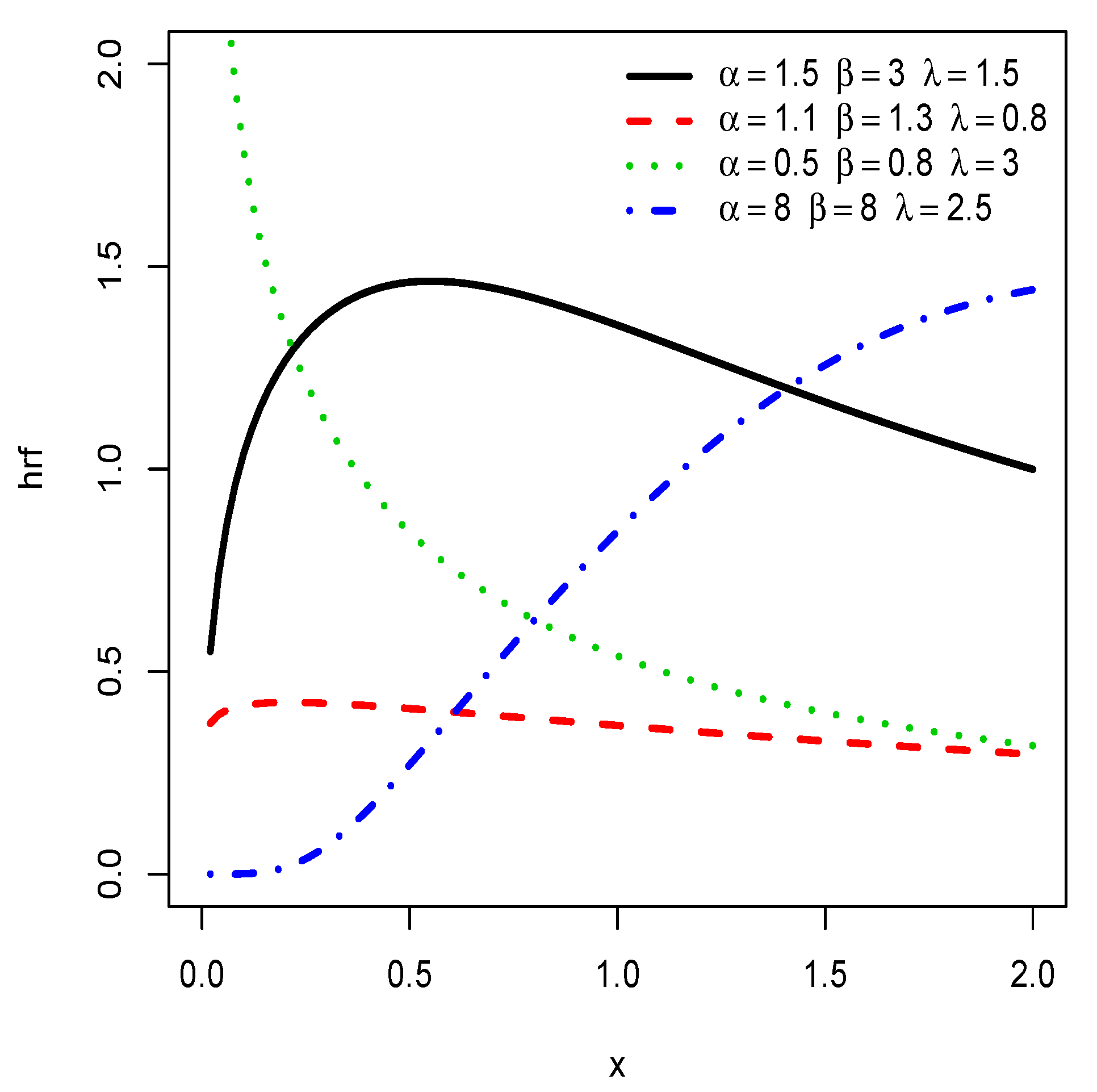
For a given $\mathbf{\varphi }$, the critical points for $h(x;\mathbf{\varphi })$ can be determined numerically by using a mathematical software. Also, the fine shape analysis for $h(x;\mathbf{\varphi })$ requires its first and second order derivatives with respect to x. The complexity of these functions is an obstacle to determine the exact range of values of the parameters characterizing the different shapes. A graphic approach is thus preferred. Thats is, in order to illustrate its flexibility, Figure 3 displays some plots of $h(x;\mathbf{\varphi })$ for some different values of the parameters.

Figure 3. Plots of the hrf of the HLIL distribution for various choices of $\alpha$, $\beta$ and $\lambda$.

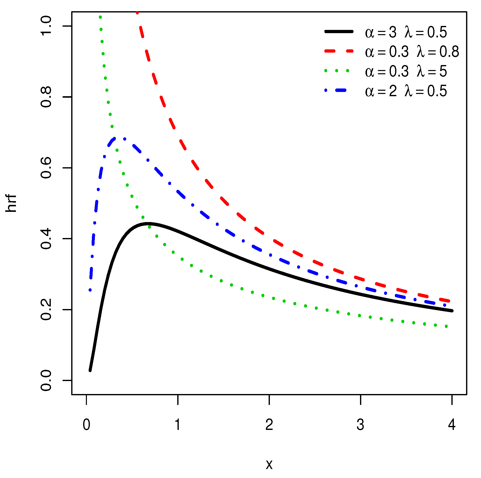
We notice that the hrf shows decreasing, ‘concave increasing’ and upside down bathtub shapes, as well as almost constant shapes. It is worth mentioning that the ‘concave increasing’ and almost constant shapes are not clearly observed for the IL distribution, as illustrated in Figure 4.

Figure 4. Plots of the hrf of the IL distribution for various choices of $\alpha$ and $\lambda$.

2.3. Quantile Function with Applications

The quantile function (qf) of the HLIL distribution, say $Q(u,\mathbf{\varphi })$, is given by the following non-linear equation: $F\left(Q\right(u;\mathbf{\varphi });\mathbf{\varphi })=u$ with $u\in (0,1)$. After some algebra, we get

$$\begin{array}{c}\hfill Q(u;\mathbf{\varphi })=\frac{1}{\lambda }{\left\{{\left[1-{\left(\frac{1-u}{1+u}\right)}^{1/\beta }\right]}^{-1/\alpha }-1\right\}}^{-1},u\in (0,1),\lambda ,\alpha ,\beta >0.\end{array}$$

(6)

The quartiles are given by $Q_1=Q(1/4;\mathbf{\varphi })$, $Q_2=Q(1/2;\mathbf{\varphi })$ and $Q_3=Q(3/4;\mathbf{\varphi })$. In particular, the median of the HLIL distribution is given by

$$M=Q_2=\frac{1}{\lambda }{\left\{{\left[1-{\left(\frac{3}{4}\right)}^{1/\beta }\right]}^{-1/\alpha }-1\right\}}^{-1}.$$

Skewness and kurtosis measures can be defined from the qf such as the Bowley skewness described by [17] and the Moors kurtosis introduced by [18]. They are, respectively, defined by

$$B\left(\mathbf{\varphi }\right)=\frac{Q(1/4;\mathbf{\varphi })-2Q(1/2;\mathbf{\varphi })+Q(3/4;\mathbf{\varphi })}{Q(3/4;\mathbf{\varphi })-Q(1/4;\mathbf{\varphi })}$$

and

$$M\left(\mathbf{\varphi }\right)=\frac{Q(7/8;\mathbf{\varphi })-Q(5/8;\mathbf{\varphi })+Q(3/8;\mathbf{\varphi })-Q(1/8;\mathbf{\varphi })}{Q(6/8;\mathbf{\varphi })-Q(2/8;\mathbf{\varphi })}.$$

The sign of $B\left(\mathbf{\varphi }\right)$ is informative on the ‘direction’ of the skewness (left skewed if $B\left(\mathbf{\varphi }\right)<0$, right-skewed if $B\left(\mathbf{\varphi }\right)>0$ and almost symmetrical if $B\left(\mathbf{\varphi }\right)=0$). As a complementary indicator, the value of $M\left(\mathbf{\varphi }\right)$ indicates the ‘tailedness’ of the distribution. The advantages of these measures are that they always exist and that they are easy to calculate. Also, they are not influenced by possible extreme tails of the distribution, contrary to the skewness and kurtosis measures defined via the moments.

3. Statistical Properties

This section deals with some fundamental properties of the HLIL distribution.

3.1. Stochastic Orders

We now investigate a first-order stochastic dominance property satisfied by the HLIL distribution, according to the concept described in [19]. Let ${\mathbf{\varphi }}_1=({\alpha }_1,{\lambda }_1,{\beta }_1)$ and ${\mathbf{\varphi }}_2=({\alpha }_2,{\lambda }_2,{\beta }_2)$. Then, if ${\alpha }_2\le {\alpha }_1$, ${\lambda }_1\le {\lambda }_2$ and ${\beta }_1\le {\beta }_2$, we have

$$\begin{array}{c}\hfill F(x;{\mathbf{\varphi }}_1)\le F(x;{\mathbf{\varphi }}_2).\end{array}$$

(7)

The proof of (7) is given in the Appendix A. Thus, under the considered configuration on ${\mathbf{\varphi }}_1$ and ${\mathbf{\varphi }}_2$, the HLIL distribution with parameter vector ${\mathbf{\varphi }}_1$ first-order stochastically dominates the HLIL distribution with parameter vector ${\mathbf{\varphi }}_2$. Also, we can use this result to show that, for $\beta \in (0,1]$, the HLIL distribution with parameter vector $\mathbf{\varphi }=(\alpha ,\lambda ,\beta )$ first-order stochastically dominates the IL distribution with parameter vector $(\alpha ,\lambda )$. Such property is not immediate for the case $\beta >1$.

3.2. Two Important Representations

In this subsection, we present two important linear representations of some functions related to the HLIL distribution. First of all, for any $\tau \in \mathbb{R}$, the following representation hold:

$$\begin{array}{c}\hfill f{(x;\mathbf{\varphi })}^{\tau }=\sum _{k,\ell =0}^{+\infty }{u}_{k,\ell }^{\left[\tau \right]}{x}^{-2\tau }{\left(1+\frac{x^{-1}}{\lambda }\right)}^{-\alpha (\ell +\tau )-\tau },\end{array}$$

(8)

where

$$\begin{array}{c}\hfill u_{k,\ell }^{\left[\tau \right]}={\left(\frac{2\beta \alpha }{\lambda }\right)}^{\tau }\left(\genfrac{}{}{0pt}{}{-2\tau }{k}\right)\left(\genfrac{}{}{0pt}{}{\beta (k+\tau )-\tau }{\ell }\right){(-1)}^{\ell }\end{array}$$

and $\left(\genfrac{}{}{0pt}{}{b}{a}\right)$ denotes the general binomial coefficient number. The proof of (8) is given in Appendix A. The decomposition of $f(x;\mathbf{\varphi })$ follows by taking $\tau =1$. In this case, note that we have

$$\begin{array}{c}\hfill u_{k,\ell }^{\left[1\right]}=\frac{2\beta \alpha }{\lambda }\left(\genfrac{}{}{0pt}{}{\beta (k+1)-1}{\ell }\right){(-1)}^{k+\ell }(k+1).\end{array}$$

Another important linear representation involving the pdf and sf of the HLIL distribution is presented below. For any $\tau \in \mathbb{R}$, we have

$$\begin{array}{c}\hfill R{(x;\mathbf{\varphi })}^{\tau }f(x;\mathbf{\varphi })=\sum _{k=0}^{+\infty }\sum _{\ell =1}^{+\infty }{w}_{k,\ell }^{\left[\tau \right]}{x}^{-2}{\left(1+\frac{x^{-1}}{\lambda }\right)}^{-\alpha \ell -1},\end{array}$$

(9)

where

$$\begin{array}{c}\hfill w_{k,\ell }^{\left[\tau \right]}=\frac{2^{\tau +1}\alpha }{\lambda (\tau +1)}\left(\genfrac{}{}{0pt}{}{-(\tau +1)}{k}\right)\left(\genfrac{}{}{0pt}{}{\beta (k+\tau +1)}{\ell }\right){(-1)}^{\ell +1}\ell .\end{array}$$

The proof of (9) is also postponed in Appendix A.

3.3. Moments

The r-th raw moment (about the origin) of the HLIL distribution exists if and only if $r<\beta$. In the next, it is supposed that r can be negative, dealing with the $(-r)$-th inverse raw moment. Then, the r-th raw moment is given by

$$\begin{array}{c}\hfill {\mu }_r^{\prime }={\int }_{-\infty }^{+\infty }{x}^{r}f(x;\mathbf{\varphi })dx={\int }_0^{+\infty }\frac{\frac{2\beta \alpha }{\lambda }{x}^{r-2}{\left(1+\frac{x^{-1}}{\lambda }\right)}^{-\alpha -1}{\left[1-{\left(1+\frac{x^{-1}}{\lambda }\right)}^{-\alpha }\right]}^{\beta -1}}{{\left\{1+{\left[1-{\left(1+\frac{x^{-1}}{\lambda }\right)}^{-\alpha }\right]}^{\beta }\right\}}^2}dx.\end{array}$$

Numerical integration method can be used to calculate this integral. Otherwise, if $r<min(1,\beta )$, r being possibly negative, the following series expansion holds:

$$\begin{array}{c}\hfill {\mu }_r^{\prime }=\sum _{k,\ell =0}^{+\infty }{u}_{k,\ell }^{\left[1\right]}{\lambda }^{1-r}B(1-r,\alpha (\ell +1)+r),\end{array}$$

(10)

where $B(x,y)={\int }_0^1{t}^{x-1}{(1-t)}^{y-1}dt$ (the so-called beta function). The proof of (10) is also postponed in Appendix A. The advantage of this expression is to be manageable for the computational point of view with a control of the errors; More N is large, more the following approximation is precise:

$$\begin{array}{c}\hfill {\mu }_r^{\prime }\approx \sum _{k,\ell =0}^N{u}_{k,\ell }^{\left[1\right]}{\lambda }^{1-r}B(1-r,\alpha (\ell +1)+r).\end{array}$$

From the raw moments, among others, we can define several measures describing important features of the HLIL distribution, such as the variance given by ${\sigma }^2={\mu }_2^{\prime }-{\left({\mu }_1^{\prime }\right)}^2$, as well as the following skewness and kurtosis measures:

$$\mathrm{skewness}=\frac{{\mu }_3^{\prime }-3{\mu }_2^{\prime }{\mu }_1^{\prime }+2{\left({\mu }_1^{\prime }\right)}^3}{{\sigma }^3},\mathrm{kurtosis}=\frac{{\mu }_4^{\prime }-4{\mu }_3^{\prime }{\mu }_1^{\prime }+6{\mu }_2^{\prime }{\left({\mu }_1^{\prime }\right)}^2-3{\left({\mu }_1^{\prime }\right)}^4}{{\sigma }^4},$$

provided that there exist.

Numerical values of first four-moments, variance, skewness and kurtosis of the HLIL distribution for $\lambda =0.5$ and some choice values of $\alpha$ and $\beta$ are displayed in Table 1 and Table 2.

Table 1. Moments, variance, skewness and kurtosis of the HLIL distribution for various values of the parameters.

${\mathit{\mu }}_{\mathit{r}}^{\prime }$	($\mathit{\alpha }=0.5,\mathit{\beta }=5$)	($\mathit{\alpha }=1,\mathit{\beta }=5$)	($\mathit{\alpha }=1.5,\mathit{\beta }=5$)	($\mathit{\alpha }=2,\mathit{\beta }=5$)	($\mathit{\alpha }=2.5,\mathit{\beta }=5$)	($\mathit{\alpha }=3,\mathit{\beta }=5$)
${\mu }_1^{\prime }$	0.191	0.723	1.359	2.033	2.725	3.426
${\mu }_2^{\prime }$	0.14	1.17	3.487	7.191	12.312	18.864
${\mu }_3^{\prime }$	0.26	3.842	16.612	45.03	95.671	175.138
${\mu }_4^{\prime }$	1.399	31.772	186.592	640.474	1648	3545
${\sigma }^2$	0.103	0.648	1.64	3.056	4.886	7.126
skewness	5.835	3.955	3.53	3.366	3.287	3.242
kurtosis	114.842	56.072	46.356	42.979	41.411	40.557

Table 2. Moments, variance, skewness and kurtosis of the HLIL distribution for various values of the parameters.

${\mathit{\mu }}_{\mathit{r}}^{\prime }$	($\mathit{\alpha }=3,\mathit{\beta }=6$)	($\mathit{\alpha }=3,\mathit{\beta }=8$)	($\mathit{\alpha }=3,\mathit{\beta }=10$)	($\mathit{\alpha }=3,\mathit{\beta }=12$)	($\mathit{\alpha }=3,\mathit{\beta }=15$)	($\mathit{\alpha }=3,\mathit{\beta }=20$)
${\mu }_1^{\prime }$	2.923	2.331	1.988	1.76	1.53	1.292
${\mu }_2^{\prime }$	12.846	7.597	5.31	4.058	2.989	2.077
${\mu }_3^{\prime }$	84.961	33.621	18.34	11.753	7.142	3.982
${\mu }_4^{\prime }$	923.833	204.7	81.428	42.193	20.498	8.918
${\sigma }^2$	4.304	2.163	1.357	0.959	0.648	0.408
skewness	2.493	1.83	1.51	1.313	1.124	0.936
kurtosis	19.977	10.753	7.947	6.611	5.554	4.697

From Table 1 and Table 2, the following remarks can be formulated.

• When $\lambda$ and $\beta$ are constant and $\alpha$ increases, the considered measures increase.
• When $\lambda$ and $\alpha$ are constant and $\beta$ increases, the considered measures decrease.
• The HLIL distribution is mainly right-skewed with consequent variations on the skewness coefficient.
• The HLIL distribution is mainly leptokurtic; the value of the kurtosis can be close to 3 (the mesokurtic case) and have very large value; It is observed the value of $114.842$ for $\lambda =0.5$, $\alpha =0.5$ and $\beta =5$.

3.4. Incomplete Moments

The r-th incomplete moment of the HLIL distribution with positive truncated parameter t always exists, and it is given by

$$\begin{array}{c}\hfill {\mu }_r^{\prime }\left(t\right)={\int }_{-\infty }^t{x}^{r}f(x;\mathbf{\varphi })dx={\int }_0^t\frac{\frac{2\beta \alpha }{\lambda }{x}^{r-2}{\left(1+\frac{x^{-1}}{\lambda }\right)}^{-\alpha -1}{\left[1-{\left(1+\frac{x^{-1}}{\lambda }\right)}^{-\alpha }\right]}^{\beta -1}}{{\left\{1+{\left[1-{\left(1+\frac{x^{-1}}{\lambda }\right)}^{-\alpha }\right]}^{\beta }\right\}}^2}dx.\end{array}$$

This integral can be managed numerically without problem. As a mathematical approach involving sums of coefficients, using (8) and proceeding as in (10), we get

$$\begin{array}{c}\hfill {\mu }_r^{\prime }\left(t\right)=\sum _{k,\ell =0}^{+\infty }{u}_{k,\ell }^{\left[1\right]}{\lambda }^{1-r}{B}_{{(1+\lambda t)}^{-1}}^{*}(1-r,\alpha (\ell +1)+r),\end{array}$$

where $B_z^{*}(x,y)={\int }_z^1{t}^{x-1}{(1-t)}^{y-1}dt$ (the so-called upper incomplete beta function). An approximation of ${\mu }_r^{\prime }\left(t\right)$ follows by substituting the infinite bound by any large integer number.

The incomplete moments are important tools to express some other quantities, as the mean deviation about the mean defined by $D_1=2{\mu }_1^{\prime }F({\mu }_1^{\prime };\mathbf{\varphi })-2{\mu }_1^{\prime }\left({\mu }_1^{\prime }\right)$ and the mean deviation about the median defined by $D_2={\mu }_1^{\prime }-2{\mu }_1^{\prime }\left(M\right)$. One can also mention the r-th lower conditional moment defined by ${\mu }_r^{\nabla }\left(t\right)={\left[F(t;\mathbf{\varphi })\right]}^{-1}{\mu }_r^{\prime }\left(t\right)$, $t\ge 0$ and the r-th upper conditional moment defined by ${\mu }_r^{▵}\left(t\right)={\left[R(t;\mathbf{\varphi })\right]}^{-1}[{\mu }_s^{\prime }-{\mu }_r^{\prime }\left(t\right)]$, $t\ge 0$. Several other functions of importance can be expressed in a similar fashion (see, for instance, [20]).

3.5. Rényi and q-Entropies

This section is devoted to the Rényi entropy and the q-entropy of the HLIL distribution. For the former definitions and applications, we refer the reader to [21,22], respectively. First of all, the Rényi entropy of the HLIL distribution not always exists; it is required that $\delta (1-\alpha )<1$ and $\delta (\beta +1)>1$, and, for $\delta \ne 1$ and $\delta >0$, it is given by

$$\begin{array}{cc}\hfill & I_{\delta }={(1-\delta )}^{-1}log\left[{\int }_{-\infty }^{+\infty }f{(x;\mathbf{\varphi })}^{\delta }dx\right]\hfill \\ \hfill & ={(1-\delta )}^{-1}log\left[{\int }_0^{+\infty }\frac{{\left(\frac{2\beta \alpha }{\lambda }\right)}^{\delta }{x}^{-2\delta }{\left(1+\frac{x^{-1}}{\lambda }\right)}^{-\delta (\alpha +1)}{\left[1-{\left(1+\frac{x^{-1}}{\lambda }\right)}^{-\alpha }\right]}^{\delta (\beta -1)}}{{\left\{1+{\left[1-{\left(1+\frac{x^{-1}}{\lambda }\right)}^{-\alpha }\right]}^{\beta }\right\}}^{2\delta }}dx\right].\hfill \end{array}$$

(11)

A numerical approach of this integral remains possible. Otherwise, for a mathematical treatment, we can use (8) with $\tau =\delta$; By proceeding as (10), there comes

$$\begin{array}{c}\hfill I_{\delta }={(1-\delta )}^{-1}log\left[\sum _{k,\ell =0}^{+\infty }{u}_{k,\ell }^{\left[\delta \right]}{\lambda }^{2\delta -1}B(2\delta -1,\alpha (\ell +\delta )-\delta +1)\right].\end{array}$$

Table 3 shows some numerical values for $I_{\delta }$ according to various values for $\mathbf{\varphi }$ and $\delta$.

Table 3. Values of the Rényi entropy of the HLIL distribution for some parameter values.

$\mathit{\alpha }$	$\mathit{\lambda }$	$\mathit{\beta }$	Rényi Entropy
			$\mathit{\delta }=\mathbf{1.2}$	$\mathit{\delta }=\mathbf{1.5}$	$\mathit{\delta }=\mathbf{2}$
1.2	0.5	1.5	141.958	78.722	57.638
1.5	0.5	1.5	141.07	78.279	57.343
2	0.5	1.5	139.945	77.716	56.968
3	0.5	1.5	138.36	76.924	56.44
4	0.5	1.5	137.236	76.362	56.065
5	0.5	1.5	136.364	75.926	55.774
1.5	0.5	1.8	166.843	91.16	65.929
1.5	0.5	2	184.062	99.767	71.667
1.5	0.5	3	270.459	142.963	100.464
1.5	0.5	4	357.156	186.311	129.363
1.5	0.5	5	444.021	229.744	158.318

Wide range of values are obtained, showing the strong effect of the parameters on the amount of information measured by $I_{\delta }$.

The q-entropy of the HLIL distribution can be determined in a similar manner. Indeed, for $q(1-\alpha )<1$ and $q(\beta +1)>1$, and, $q\ne 1$ and $q>0$, it is given by

$$\begin{array}{c}\hfill H_q={(q-1)}^{-1}\left[1-{\int }_{-\infty }^{+\infty }f{(x;\mathbf{\varphi })}^{q}dx\right].\end{array}$$

Therefore, by replacing $\delta$ by q in some developments for $I_{\delta }$, we get

$$\begin{array}{c}\hfill H_q={(q-1)}^{-1}\left[1-\sum _{k,\ell =0}^{+\infty }{u}_{k,\ell }^{\left[q\right]}{\lambda }^{2q-1}B(2q-1,\alpha (\ell +q)-q+1)\right].\end{array}$$

As a numerical approach, we present some numerical values for $H_q$ for selected values of the parameters in Table 4.

Table 4. Values of the q-entropy of the HLIL distribution for some parameter values.

$\mathit{\alpha }$	$\mathit{\lambda }$	$\mathit{\beta }$	q-Entropy
			$\mathit{q}=\mathbf{1.2}$	$\mathit{q}=\mathbf{1.5}$	$\mathit{q}=\mathbf{2}$
1.2	2	1.5	1.027	0.757	0.529
1.5	2	1.5	1.230	0.914	0.643
2	2	1.5	1.462	1.075	0.743
3	2	1.5	1.752	1.254	0.833
4	2	1.5	1.938	1.357	0.876
5	2	1.5	2.074	1.426	0.901
1.5	2	1.8	1.002	0.759	0.546
1.5	2	2	0.873	0.665	0.481
1.5	2	3	0.385	0.267	0.155
1.5	2	4	0.048	−0.048	−0.160
1.5	2	5	−0.209	−0.312	−0.464

We also see positive and negative values, with a wide range of possible values. This indicates that the randomness of the HLIL distribution is very versatile.

3.6. Order Statistics

Order statistics are of importance in several branches of probability and statistics. Here, we determine some properties of the order statistics in the context of the HLIL distribution. Let $X_{\left(1\right)},\dots ,X_{\left(n\right)}$ be the order statistics of a random sample of size n from the HLIL distribution. Then, the pdf of $X_{\left(s\right)}$ is given by

$$\begin{array}{c}\hfill f_{\left(s\right)}(x;\mathbf{\varphi })=\frac{1}{B(s,n-s+1)}F{(x;\mathbf{\varphi })}^{s-1}R{(x;\mathbf{\varphi })}^{n-s}f(x;\mathbf{\varphi }),x>0.\end{array}$$

(12)

Hence, by substituting (3), (4) and (5) into (12), the analytical expression of $f_{\left(s\right)}(x;\mathbf{\varphi })$ is given by

$$\begin{array}{cc}\hfill f_{\left(s\right)}(x;\mathbf{\varphi })& =\frac{\frac{2^{n-s+1}\beta \alpha }{\lambda }{x}^{-2}{\left(1+\frac{x^{-1}}{\lambda }\right)}^{-\alpha -1}{\left[1-{\left(1+\frac{x^{-1}}{\lambda }\right)}^{-\alpha }\right]}^{\beta (n-s+1)-1}}{B(s,n-s+1){\left\{1+{\left[1-{\left(1+\frac{x^{-1}}{\lambda }\right)}^{-\alpha }\right]}^{\beta }\right\}}^{n+1}}\hfill \\ \hfill & \times {\left\{1-{\left[1-{\left(1+\frac{x^{-1}}{\lambda }\right)}^{-\alpha }\right]}^{\beta }\right\}}^{s-1}.\hfill \end{array}$$

A more tractable approach is the use of series expansions. Indeed, by applying the binomial theorem, it follows from (12) that

$$\begin{array}{c}\hfill f_{\left(s\right)}(x;\mathbf{\varphi })=\frac{1}{B(s,n-s+1)}\sum _{j=0}^{s-1}\left(\genfrac{}{}{0pt}{}{s-1}{j}\right){(-1)}^{j}R{(x;\mathbf{\varphi })}^{j+n-s}f(x;\mathbf{\varphi }).\end{array}$$

Now, by letting $\tau =j+n-s$ and using (9), we get

$$\begin{array}{c}\hfill f_{\left(s\right)}(x;\mathbf{\varphi })=\sum _{j=0}^{s-1}\sum _{k=0}^{+\infty }\sum _{\ell =1}^{+\infty }{z}_{k,\ell }^{[j+n-s]}{x}^{-2}{\left(1+\frac{x^{-1}}{\lambda }\right)}^{-\alpha \ell -1},\end{array}$$

where

$$\begin{array}{cc}\hfill z_{k,\ell }^{[j+n-s]}& =\frac{1}{B(s,n-s+1)}\left(\genfrac{}{}{0pt}{}{s-1}{j}\right){(-1)}^j{w}_{k,\ell }^{[j+n-s]}\hfill \\ \hfill & =\frac{2^{\tau +1}\alpha }{\lambda (\tau +1)}\frac{1}{B(s,n-s+1)}\left(\genfrac{}{}{0pt}{}{s-1}{j}\right)\left(\genfrac{}{}{0pt}{}{-(\tau +1)}{k}\right)\left(\genfrac{}{}{0pt}{}{\beta (k+\tau +1)}{\ell }\right){(-1)}^{\ell +j+1}\ell .\hfill \end{array}$$

From this result, one can determine several measures of interest, as the r-th raw moment of $X_{\left(s\right)}$. Indeed, for $r<1$ (possibly negative), by proceeding as in (10), we get

$$\begin{array}{c}\hfill {\mu }_{\left(s\right)}^{\prime }={\int }_{-\infty }^{+\infty }{x}^r{f}_{\left(s\right)}(x;\mathbf{\varphi })dx=\sum _{j=0}^{s-1}\sum _{k=0}^{+\infty }\sum _{\ell =1}^{+\infty }{z}_{k,\ell }^{[j+n-s]}{\lambda }^{1-r}B(1-r,\alpha \ell +r).\end{array}$$

Some results with potential interest on the extreme of the HLIL distribution are presented below.

The limiting distribution of the first order statistic, $X_{\left(1\right)}$, is the Weibull distribution with the following cdf: $F_{*}(x;\alpha )=1-e^{-x^{\alpha }}$, $x>0$, i.e., there exist ${\left(a_n\right)}_{n\in {\mathbb{N}}^{*}}$ and ${\left(b_n\right)}_{n\in {\mathbb{N}}^{*}}$ such that

$$\begin{array}{c}\hfill \underset{n\to +\infty }{lim}P\left(b_n(X_{\left(1\right)}-a_n)\le x\right)=F_{*}(x;\alpha ).\end{array}$$

(13)

The proof of (13) is postponed in Appendix A.

Also, the limiting distribution of the last order statistic, $X_{\left(n\right)}$, is the Fréchet distribution with the following cdf: $F_{**}(x;\beta )=e^{-x^{-\beta }}$, $x>0$, i.e., there exist ${\left(a_n\right)}_{n\in {\mathbb{N}}^{*}}$ and ${\left(b_n\right)}_{n\in {\mathbb{N}}^{*}}$ such that

$$\begin{array}{c}\hfill \underset{n\to +\infty }{lim}P\left(b_n(X_{\left(n\right)}-a_n)\le x\right)=F_{**}(x;\beta ).\end{array}$$

(14)

The proof of (14) is also given in Appendix A.

4. Different Methods of Estimation and Simulation

In this section, we turn out the HLIL distribution as a model, and we investigate the estimation of $\alpha$, $\lambda$ and $\beta$ by different notorious methods.

For the purposes of this study, $(x_1,\dots ,x_n)$ denotes a random sample of size n from the HLIL distribution. Thus, $x_1,\dots ,x_n$ represent the data, and their ascending ordering values are denoted by $x_{\left(1\right)},\dots ,x_{\left(n\right)}$.

4.1. Maximum Likelihood Estimates (MLEs)

For its theoretical properties, and its practical properties as well, the most popular estimation method remains the maximum likelihood method. The maximum likelihood estimates (MLEs) of $\mathbf{\varphi }$ are given by ${\widehat{\mathbf{\varphi }}}_{MLE}={argmax}_{\mathbf{\varphi }}L\left(\mathbf{\varphi }\right)$, where $L\left(\mathbf{\varphi }\right)$ denotes the likelihood function defined by $L\left(\mathbf{\varphi }\right)={\prod }_{i=1}^{n}f(x_i;\mathbf{\varphi })$ or, equivalently, ${\widehat{\mathbf{\varphi }}}_{MLE}={argmax}_{\mathbf{\varphi }}\ell \left(\mathbf{\varphi }\right)$, where $\ell \left(\mathbf{\varphi }\right)$ denotes the log-likelihood function defined by

$$\begin{array}{cc}\hfill \ell \left(\mathbf{\varphi }\right)& =log\left[L\left(\mathbf{\varphi }\right)\right]=\sum _{i=1}^{n}log\left[f(x_i;\mathbf{\varphi })\right]=nlog\left(2\right)+nlog\left(\beta \right)+nlog\left(\alpha \right)-nlog\left(\lambda \right)-2\sum _{i=1}^{n}log\left(x_i\right)\hfill \\ \hfill & -(\alpha +1)\sum _{i=1}^{n}log\left(1+\frac{x_i^{-1}}{\lambda }\right)+(\beta -1)\sum _{i=1}^{n}log\left[1-{\left(1+\frac{x_i^{-1}}{\lambda }\right)}^{-\alpha }\right]\hfill \\ \hfill & -2\sum _{i=1}^{n}log\left\{1+{\left[1-{\left(1+\frac{x_i^{-1}}{\lambda }\right)}^{-\alpha }\right]}^{\beta }\right\}.\hfill \end{array}$$

The differentiability of the above function can provide us the requested estimates of the parameter vector $\mathbf{\varphi }$, through the (simultaneously) solution of the three non-linear equations corresponding to $\partial \ell \left(\mathbf{\varphi }\right)/\partial \mathbf{\varphi }=0$, with respect to $\mathbf{\varphi }$. On the basis of the second partial derivative of $\ell \left(\mathbf{\varphi }\right)$, we determine the inverse observed information matrix whose diagonal elements correspond to the square of the standard errors (SEs) of the MLEs. The general formula can be found in [23].

4.2. Ordinary and Weighted Least Squares Estimates (LSEs) and (WLSEs)

The (ordinary) least squares estimates (LSEs) of $\mathbf{\varphi }$ are now investigated. They are given by ${\widehat{\mathbf{\varphi }}}_{LSE}={argmin}_{\mathbf{\varphi }}LS\left(\mathbf{\varphi }\right)$, where

$$\begin{array}{c}\hfill LS\left(\mathbf{\varphi }\right)=\sum _{i=1}^n{\left[F(x_{\left(i\right)};\mathbf{\varphi })-\frac{i}{n+1}\right]}^2=\sum _{i=1}^n{\left[\frac{1-{\left[1-{\left(1+\frac{x_{\left(i\right)}^{-1}}{\lambda }\right)}^{-\alpha }\right]}^{\beta }}{1+{\left[1-{\left(1+\frac{x_{\left(i\right)}^{-1}}{\lambda }\right)}^{-\alpha }\right]}^{\beta }}-\frac{i}{n+1}\right]}^2.\end{array}$$

They can be obtained by solving simultaneously the three non-linear equations summarized as $\partial LS\left(\mathbf{\varphi }\right)/\partial \mathbf{\varphi }=0$, with respect to $\mathbf{\varphi }$.

In a similar fashion, the weighted least squares estimates (WLSEs) of $\mathbf{\varphi }$ are defined by ${\widehat{\mathbf{\varphi }}}_{WLSE}={argmin}_{\mathbf{\varphi }}WLS\left(\mathbf{\varphi }\right)$, where

$$\begin{array}{cc}\hfill WLS\left(\mathbf{\varphi }\right)& =\sum _{i=1}^n\frac{{(n+1)}^2(n+2)}{i(n-i+1)}{\left[F(x_{\left(i\right)};\mathbf{\varphi })-\frac{i}{n+1}\right]}^2\hfill \\ \hfill & =\sum _{i=1}^n\frac{{(n+1)}^2(n+2)}{i(n-i+1)}{\left[\frac{1-{\left[1-{\left(1+\frac{x_{\left(i\right)}^{-1}}{\lambda }\right)}^{-\alpha }\right]}^{\beta }}{1+{\left[1-{\left(1+\frac{x_{\left(i\right)}^{-1}}{\lambda }\right)}^{-\alpha }\right]}^{\beta }}-\frac{i}{n+1}\right]}^2.\hfill \end{array}$$

In a similar manner to the LSEs, the WLEs can be obtained by solving simultaneously the three non-linear equations summarized as $\partial WLS\left(\mathbf{\varphi }\right)/\partial \mathbf{\varphi }=0$, with respect to $\mathbf{\varphi }$.

We refer to [24] for further detail on least squares methods in full generality.

4.3. Percentile Estimates (PCEs)

The percentile estimates (PCEs) was pioneered by [25] (for the Weibull distribution). Here, the PCEs of $\mathbf{\varphi }$ are defined by ${\widehat{\mathbf{\varphi }}}_{PCE}={argmin}_{\mathbf{\varphi }}PC\left(\mathbf{\varphi }\right)$, where

$$\begin{array}{c}\hfill PC\left(\mathbf{\varphi }\right)=\sum _{i=1}^n{\left[x_{\left(i\right)}-Q(p_i;\mathbf{\varphi })\right]}^2=\sum _{i=1}^n{\left[x_{\left(i\right)}-\frac{1}{\lambda }{\left\{{\left[1-{\left(\frac{1-p_i}{1+p_i}\right)}^{1/\beta }\right]}^{-1/\alpha }-1\right\}}^{-1}\right]}^2,\end{array}$$

where $p_i=i/(n+1)$. They can be obtained by solving simultaneously the three non-linear equations corresponding to $\partial PC\left(\mathbf{\varphi }\right)/\partial \mathbf{\varphi }=0$, with respect to $\mathbf{\varphi }$.

4.4. Cramér-Von Mises Minimum Distance Estimates (CVEs)

Following the approach described by [26], the Cramér-von Mises minimum distance estimates (CVEs) of $\mathbf{\varphi }$ are defined by ${\widehat{\mathbf{\varphi }}}_{CVE}={argmin}_{\mathbf{\varphi }}CV\left(\mathbf{\varphi }\right)$, where

$$\begin{array}{c}\hfill CV\left(\mathbf{\varphi }\right)=\frac{1}{12n}+\sum _{i=1}^n{\left[F(x_{\left(i\right)};\mathbf{\varphi })-\frac{2i-1}{2n}\right]}^2=\frac{1}{12n}+\sum _{i=1}^n{\left[\frac{1-{\left[1-{\left(1+\frac{x_{\left(i\right)}^{-1}}{\lambda }\right)}^{-\alpha }\right]}^{\beta }}{1+{\left[1-{\left(1+\frac{x_{\left(i\right)}^{-1}}{\lambda }\right)}^{-\alpha }\right]}^{\beta }}-\frac{2i-1}{2n}\right]}^2.\end{array}$$

They can be obtained by solving simultaneously the three non-linear equations summarized as $\partial CV\left(\mathbf{\varphi }\right)/\partial \mathbf{\varphi }=0$, with respect to $\mathbf{\varphi }$.

4.5. Maximum Product of Spacings Estimates (MPSEs)

The method of maximum product of spacings estimation was introduced by [27]. We now apply it in the context of the HLIL model. Let us set

$$D_i\left(\mathbf{\varphi }\right)=F(x_{\left(i\right)};\mathbf{\varphi })-F(x_{(i-1)};\mathbf{\varphi })$$

for $i=1,2,\dots ,n+1$, where, by convention, $F(x_{\left(0\right)};\mathbf{\varphi })=0$ and $F(x_{(n+1)};\mathbf{\varphi })=1$. The maximum product spacings estimates (MPSEs) of $\mathbf{\varphi }$ are defined by ${\widehat{\mathbf{\varphi }}}_{MPSE}={argmax}_{\mathbf{\varphi }}G\left(\mathbf{\varphi }\right)$, where

$$\begin{array}{c}\hfill G\left(\mathbf{\varphi }\right)={\left[\prod _{i=1}^{n+1}{D}_i\left(\mathbf{\varphi }\right)\right]}^{\frac{1}{n+1}},\end{array}$$

or, equivalently, ${\widehat{\mathbf{\varphi }}}_{MPSE}={argmax}_{\mathbf{\varphi }}LG\left(\mathbf{\varphi }\right)$, where

$$\begin{array}{c}\hfill LG\left(\mathbf{\varphi }\right)=log\left[G\left(\mathbf{\varphi }\right)\right]=\frac{1}{n+1}\sum _{i=1}^{n+1}log\left[D_i\left(\mathbf{\varphi }\right)\right].\end{array}$$

They can be obtained by solving simultaneously the three non-linear equations summarized as $\partial LG\left(\mathbf{\varphi }\right)/\partial \mathbf{\varphi }=0$, with respect to $\mathbf{\varphi }$.

4.6. Numerical Results

We now investigate the behavior of the ML, LS, WLS, PC, CV and MPS estimates presented above, as well as entropy estimates. The software Mathcad(14) is used. We generate 1000 random samples $(x_1,\dots ,x_n)$ of sizes $n=100$, 200, 300, 1000 and 2000 from the HLIL distribution via the so-called inverse transform sampling based on the qf given by (6) (see [28], for instance). The two following sets of parameters are chosen as: Set1: $(\alpha =2,\lambda =0.5,\beta =2)$ and Set2: $(\alpha =2,\lambda =0.5,\beta =3)$.

Then, the mean ML, LS, WLS, PC, CV and MPS estimates (Estim) of $\alpha$, $\beta$ and $\lambda$ are calculated, as well as their standard mean square errors (MSEs). Numerical results are shown in Table 5 and Table 6 for Set1 and Set2, respectively.

Table 5. Estimates and mean square errors (MSEs) of HLIL distribution for maximum likelihood (ML), least squares (LS), weighted least squares (WLS), percentile (PC), and maximum product of spacing (MPS) estimates for Set1: $(\alpha =2,\lambda =0.5,\beta =2)$.

n	MLE		LSE		WLSE		CVE		PCE		MPSE
	Estimates	MSEs	Estimates	MSEs	Estimates	MSEs	Estimates	MSEs	Estimates	MSEs	Estimates	MSEs
	1.964	1.985	2.34	3.311	2.33	0.96	2.625	3.398	2.083	1.443	2.257	2.645
100	0.993	1.205	0.664	0.875	0.681	0.232	0.846	1.088	0.615	0.657	0.779	0.559
	2.223	0.155	2.098	0.216	1.969	0.185	2.01	0.223	2.334	0.72	2.037	0.104
	2.051	0.922	2.091	0.343	2.171	0.275	2.465	1.143	1.876	0.379	1.874	0.913
200	0.646	0.138	0.506	0.042	0.575	0.087	0.712	0.376	0.474	0.142	0.717	0.184
	2.082	0.045	2.131	0.142	2.064	0.094	2.045	0.108	2.333	0.611	2.066	0.046
	2.175	0.68	2.1	0.269	2.035	0.221	2.063	0.192	1.873	0.303	1.938	0.573
300	0.552	0.076	0.538	0.041	0.538	0.07	0.512	0.025	0.458	0.091	0.64	0.112
	2.028	0.029	2.074	0.088	2.021	0.073	2.076	0.09	2.275	0.414	2.034	0.025
	2.04	0.061	2.063	0.076	1.968	0.018	2.136	0.09	1.947	0.108	1.976	0.035
1000	0.518	0.013	0.527	0.011	0.472	0.005	0.553	0.015	0.48	0.037	0.503	0.008
	2.011	0.023	1.994	0.022	2.06	0.019	1.961	0.016	2.137	0.175	1.974	0.023
	2.046	0.026	2.086	0.061	1.979	0.015	2.036	0.016	1.979	0.052	1.942	0.023
2000	0.519	0.006	0.539	0.01	0.489	0.004	0.511	0.004	0.488	0.018	0.474	0.004
	1.994	0.008	1.979	0.011	2.03	0.013	2.012	0.012	2.099	0.14	2.037	0.009

Table 6. Estimates and MSEs of HLIL distribution for ML, LS, WLS, CV, PC and MPS estimates for Set2: $(\alpha =2,\lambda =0.5,\beta =3)$.

n	MLE		LSE		WLSE		CVE		PCE		MPSE
	Estimates	MSEs	Estimates	MSEs	Estimates	MSEs	Estimates	MSEs	Estimates	MSEs	Estimates	MSEs
	1.957	1.01	3.141	3.554	2.302	0.621	2.447	2.234	2.023	1.266	2.182	1.843
100	0.783	0.449	1.05	0.931	0.639	0.1	0.705	0.505	0.64	0.761	0.682	0.227
	3.198	0.223	2.966	0.505	2.951	0.295	2.939	0.363	3.32	1.647	3.037	0.156
	1.951	0.646	2.571	1.413	2.156	0.27	2.224	0.316	2.076	0.898	1.854	0.539
200	0.659	0.134	0.761	0.268	0.583	0.062	0.635	0.1	0.579	0.394	0.696	0.19
	3.103	0.079	2.857	0.262	2.975	0.265	2.958	0.351	3.39	1.216	3.075	0.086
	1.86	0.371	2.306	0.651	2.182	0.113	2.297	0.18	2.041	0.288	1.763	0.3
300	0.626	0.066	0.7	0.253	0.605	0.025	0.638	0.041	0.575	0.127	0.67	0.117
	3.092	0.051	2.86	0.257	2.806	0.122	2.888	0.215	3.134	1.039	3.082	0.057
	2.039	0.05	2.126	0.048	2.128	0.044	2.202	0.08	2.013	0.097	1.982	0.028
1000	0.52	0.013	0.583	0.014	0.579	0.014	0.611	0.02	0.528	0.037	0.506	0.008
	3.015	0.042	2.792	0.104	2.874	0.108	2.836	0.095	2.992	0.327	2.977	0.041
	2.044	0.022	2.117	0.039	2.113	0.024	2.136	0.042	2.003	0.043	1.957	0.021
2000	0.521	0.006	0.589	0.014	0.588	0.014	0.578	0.012	0.513	0.017	0.478	0.005
	2.984	0.032	2.835	0.06	2.837	0.048	2.843	0.066	3.003	0.271	3.069	0.035

From Table 5 and Table 6, we notice the following facts.

• For all estimates, as expected, the MSEs decrease as sample sizes increase.
• The MSEs of the MPSEs of $\mathbf{\varphi }$ take the lowest value among the corresponding MSEs for the other methods in almost all cases. Other details are given below.

  –

  For the MLEs, when $\beta$ increases, the MSEs for $\alpha$ and $\lambda$ decrease but the MSE for $\beta$ is increasing.

  –

  For the LSEs, when $\beta$ increases, the MSEs for $\alpha$, $\lambda$ and $\beta$ are increasing.

  –

  For the WLSEs, when $\beta$ increases, the MSEs for $\alpha$ and $\lambda$ are decreasing but the MSE for $\beta$ is increasing.

  –

  For the CVEs, when $\beta$ increases, the MSEs for $\alpha$ and $\lambda$ are decreasing but the MSE for $\beta$ is increasing

  –

  For the the PCEs, when $\beta$ increases, the MSEs for $\alpha$, $\lambda$ and $\beta$ are increasing except for $\alpha$ at $n=100$ where they decrease.

  –

  For the MPSEs, when $\beta$ increases, the MSEs for $\alpha$ and $\lambda$ are decreasing but the MSE for $\beta$ is increasing.

We complete this part by performing a simulation study on the estimation of the Rényi entropy $I_{\delta }$ defined by (11) for various values of $\delta$: $\delta =0.5$, $\delta =1.5$ and $\delta =2.5$. We consider the same framework as above, the ML estimates of $\alpha$, $\beta$ and $\lambda$, as well as the plugging principle. Then, we determine the exact values of the entropy, estimates and the relative biases (RBs) defined by the generic formula: RB = mean of (Estimate − Exact value)/Exact value. The numerical results are collected in Table 7 and Table 8 for Set1 and Set2, respectively.

Table 7. Rényi entropy estimates for Set1.

n	$\mathit{\delta }=0.5$			$\mathit{\delta }=1.5$			$\mathit{\delta }=2.5$
	Exact Value	Estimates	RB	Exact Value	Estimates	RB	Exact Value	Estimates	RB
100		−16.078	0.32		110.569	0.117		68.301	0.104
200		−13.631	0.119		103.169	0.042		64.19	0.037
300	−12.18	−12.627	0.037	99.018	100.113	0.011	61.884	62.492	0.01
1000		−12.406	0.019		99.467	0.005		62.134	0.004
2000		−12.162	0.001		98.741	0.003		61.73	0.002

Table 8. Rényi entropy estimates for Set2.

n	$\mathit{\delta }=0.5$			$\mathit{\delta }=1.5$			$\mathit{\delta }=2.5$
	Exact Value	Estimates	RB	Exact Value	Estimates	RB	Exact Value	Estimates	RB
100		−30.078	0.132		152.297	0.073		91.483	0.068
200		−28.502	0.072		147.556	0.04		88.849	0.037
300	−26.58	−28.237	0.062	141.838	146.74	0.035	85.673	88.396	0.032
1000		−26.808	0.009		142.427	0.004		86	0.004
2000		−26.363	0.008		141.198	0.004		85.361	0.004

As expected, from Table 7 and Table 8, we notice that, when the sample sizes increase, the RBs of the Rényi entropy decrease. Also

• when $\delta$ increases, the RBs of the Rényi entropy decrease.
• when $\beta$ increases, the RBs of the Rényi entropy decrease.

5. Applications

In this section, we show the interest of the HLIL distribution using three real data sets in the field of environment, engineering and insurance. The data sets are presented below.

The first data set is obtained from [29]. It consists of 30 successive values of March precipitation in Minneapolis. The measurements are in inches. The data are given by: 0.77, 1.74, 0.81, 1.20, 1.95, 1.20, 0.47, 1.43, 3.37, 2.20, 3.00, 3.09, 1.51, 2.10, 0.52, 1.62, 1.31, 0.32, 0.59, 0.81, 2.81, 1.87, 1.18, 1.35, 4.75, 2.48, 0.96, 1.89, 0.90, 2.05.

The second data set is the Aircraft Windshield data set by [30]. The data consist of the failure times of 84 Aircraft Windshield. The unit for measurement is 1000 h.The data are given by: 0.040, 1.866, 2.385, 3.443, 0.301, 1.876, 2.481, 3.467, 0.309, 1.899, 2.610, 3.478, 0.557, 1.911, 2.625, 3.578, 0.943, 1.912, 2.632, 3.595, 1.070, 1.914, 2.646, 3.699, 1.124, 1.981, 2.661, 3.779, 1.248, 2.010, 2.688, 3.924, 1.281, 2.038, 2.823, 4.035, 1.281, 2.085, 2.890, 4.121, 1.303, 2.089, 2.902, 4.167, 1.432, 2.097, 2.934, 4.240, 1.480, 2.135, 2.962, 4.255, 1.505, 2.154, 2.964, 4.278, 1.506, 2.190, 3.000, 4.305, 1.568, 2.194, 3.103, 4.376, 1.615, 2.223, 3.114, 4.449, 1.619, 2.224, 3.117, 4.485, 1.652, 2.229, 3.166, 4.570, 1.652, 2.300, 3.344, 4.602, 1.757, 2.324, 3.376, 4.663. The third data set is a heavy-tailed real data set from the insurance industry. This data set represents monthly unemployment insurance measures from July 2008 to April 2013 including 58 sightings, and it is reported by the ministry of Labor, Licensing and Regulation (LLR), State of Maryland, USA. The data consist of 21 variables and we analyze in particular the twelfth variable (number 12). The data are available at: https://catalog.data.gov/dataset/unemploymentinsurance-data-july-2008-to-april-2013 (accessed on the 3 February 2021).

Then, the fits of the HLIL model are compared with those of some competitive models such as inverse Lomax (IL), Topp-Leone inverse Lomax (TIL) by [31], Weibull inverse Lomax (WIL) by [11], Kumaraswamy Lomax (KL) by [32], beta Lomax (BL) by [33] and exponentiated power Lomax (EPL) by [34]. The maximum likelihood method is considered, mainly thanks to its attractive theoretical and computational properties. We compute the well-known statistical measures, namely Akaike information criterion (AIC), Bayesian information criterion (BIC), Anderson-Darling (AD) and Cramér-von Mises (CVM). As usual, the model with a lower value for AIC, BIC, CVM and AD should be the preferred model. The results, described below, are obtained by using the R software.

Table 9, Table 10 and Table 11 present the MLEs and their SEs (in parentheses) for the first, second and third data sets, respectively.

Table 9. Maximum Likelihood Estimates (MLEs) with their standard errors (SEs) for the first data set.

Model	MLEs and SEs
HLIL	3.3774	7.9710	0.8085	-
($\alpha ,\beta ,\lambda$)	(0.1673)	(0.0245)	(0.4986)	-
EPL	25.2967	0.7590	12.7190	7.9758
($\alpha ,\beta ,\lambda ,a$)	(4.0719)	(0.0341)	(12.6748)	(0.1906)
WIL	0.0024	2.0529	0.0604	2.5469
($a,b,\lambda ,\beta$)	(0.0005)	(0.2048)	(0.0216)	(0.0501)
TIL	11.6699	0.3946	1.0885	-
($\alpha ,\beta ,\lambda$)	(4.6202)	(0.6050)	(3.0847)	-
IL	0.0210	54.8749	-	-
($\alpha ,\lambda$)	(0.0348)	(0.0946)	-	-

Table 10. MLEs with their SEs for the second data set.

Model	MLEs and SEs
HLIL	2.2493	139.8835	0.0532	-
($\alpha ,\beta ,\lambda$)	(0.2886)	(7.0477)	(0.0337)	-
KwL	3.2372	11.9966	3.2456	9.1600
($\alpha ,\beta ,a,b$)	(2.4802)	(16.4620)	(1.0686)	(5.3663)
BL	165.2269	5.1558	3.5609	43.6788
($c,k,a,b$)	(5.9677)	(0.6954)	(0.5250)	(8.0152)
WIL	0.0027	1.5655	0.0606	1.1832
($a,b,\lambda ,\beta$)	(0.0004)	(0.2026)	(0.0179)	(0.8351)
TIL	3.9207	1.4443	1.0833	-
($\alpha ,\beta ,\lambda$)	(3.5674)	(0.6032)	(0.8878)	-
IL	0.5031	4.0306	-	-
($\alpha ,\lambda$)	(0.1892)	(1.2907)	-	-

Table 11. MLEs with their SEs for the third data set.

Model	MLEs and SEs
HLIL	37.9868	12.1643	0.2301	-
($\alpha ,\beta ,\lambda$)	(3.9893)	(1.2670)	(0.2570)	-
EPL	25.5454	0.6161	96.1370	15.6028
($\alpha ,\beta ,\lambda ,a$)	(2.7281)	(0.7262)	(0.3338)	(3.0301)
WIL	0.0026	0.6577	0.0116	0.5668
($a,b,\lambda ,\beta$)	(0.0005)	(0.0476)	(0.0044)	(0.2457)
TIL	56.5719	1.1760	7.0916	-
($\alpha ,\beta ,\lambda$)	(5.3292)	(0.8181)	(0.0656)	-
IL	1.5381	40.4936	-	-
($\beta ,\lambda$)	(1.2669)	(3.3980)	-	-

Table 12, Table 13 and Table 14 inform on the values of the AIC, BIC, AD and CVM for the first, second and third data sets, respectively.

Table 12. The Akaike information criterion (AIC), Bayesian information criterion (BIC), Anderson-Darling (AD), and Cramér-von Mises (CVM) values for the first data set.

Model	AIC	BIC	AD	CVM
HLIL	82.3694	86.5730	0.1070	0.0147
EPL	84.8304	90.4352	0.1760	0.0272
WIL	96.1966	101.8014	0.2459	0.0329
TIL	86.9198	91.1234	0.4658	0.0751
IL	96.8127	99.6151	0.5066	0.0817

Table 13. The AIC, BIC, AD and CVM values for the second data set.

Model	AIC	BIC	AD	CVM
HLIL	268.8231	276.1510	0.5765	0.0567
KwL	280.4553	290.2259	1.0633	0.1175
BL	285.2487	295.0193	1.3961	0.1662
WIL	331.6880	341.4586	0.5802	0.0552
TIL	328.0861	335.4140	3.9985	0.5999
IL	365.4879	370.3732	5.4250	0.8625

Table 14. The AIC, BIC, AD and CVM values for the third data set.

Model	AIC	BIC	AD	CVM
HLIL	537.6881	543.8695	0.7968	0.1396
EPL	565.9949	574.2367	1.0505	0.1939
WIL	670.4852	678.7270	1.5208	0.2809
TIL	559.5491	565.7304	0.8901	0.1580
IL	613.7669	617.8878	1.2920	0.2223

Since it has the smallest values for all these criteria, one can consider that the HLIL model is the best. In particular, for all the considered criteria, and the three data sets, we notice that the HLIL model significantly dominates the former IL model. On the basis of these criteria, the superiority of the HLIL model over the competitors is particularly obvious for the fit of the third data set.

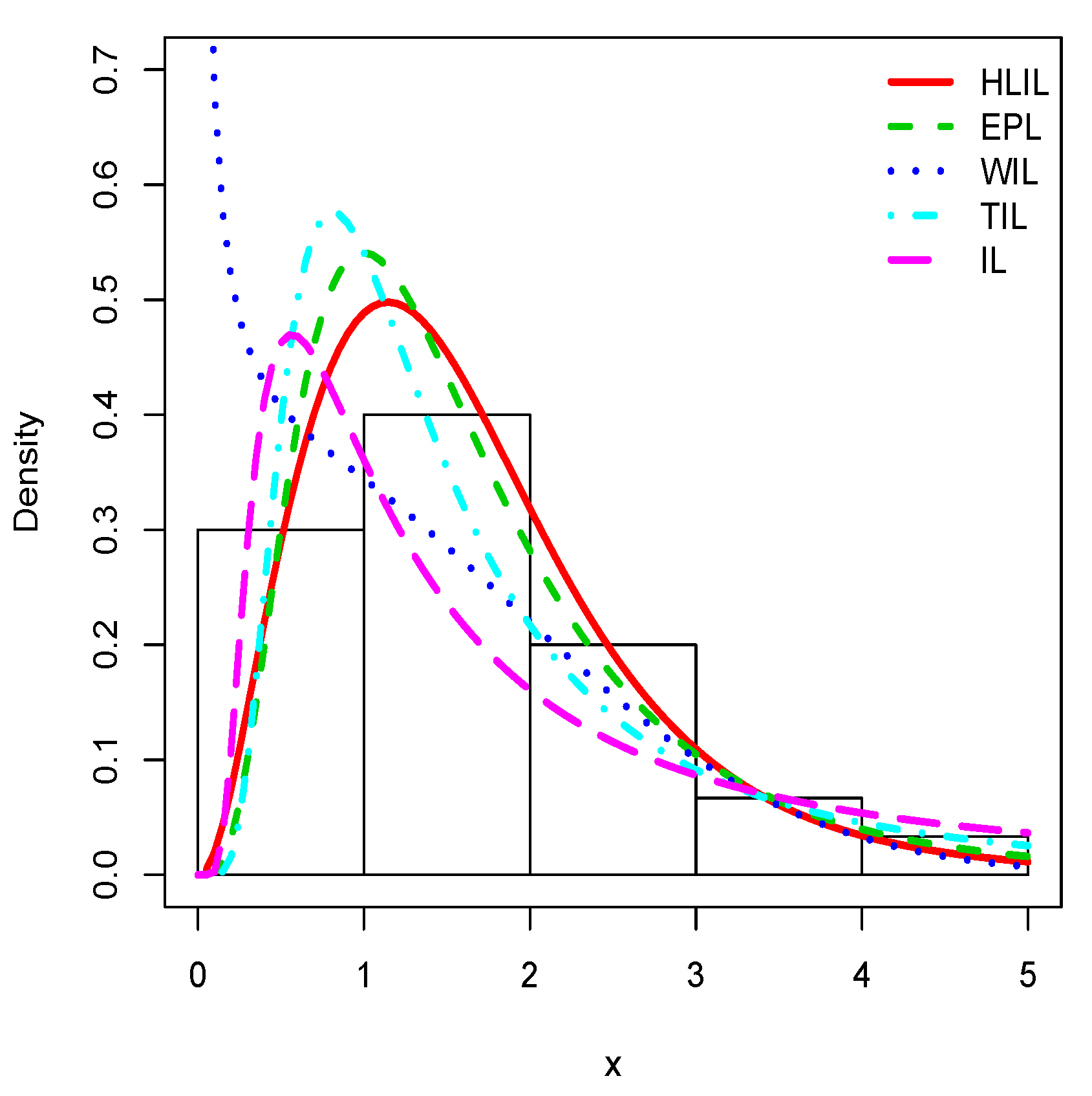
Figure 5, Figure 6 and Figure 7 illustrate the estimated pdfs with superposition over the related histograms for the first, second and third data sets, respectively.

Figure 5. Plots of the estimated pdfs for the first data set.

Figure 6. Plots of the estimated pdfs for the second data set.

Figure 7. Plots of the estimated pdfs for the thrid data set.

Visually, it is clear that the fit of the HLIL distribution is more adequate. The high flexibility of the peak and tails of the pdf of the HLIL distribution is clearly the key to success in terms of adaptability, far beyond the modeling ability of the former IL distribution. Moreover, for the third data set, as illustrated by Figure 7, the adaptive power of the HLIL is particularly dominant.

6. Concluding Remarks

In this article, a new three-parameter distribution, called the HLIL distribution, is introduced. It aims to provide a workable extension of the IL distribution with more advantages for the modeling of heavy-tailed data. These advantages include more flexibility in the peak and tails of the former IL distribution. Some statistical properties of the proposed distribution such as first-order stochastic dominance, moments, Rényi and q-entropies and order statistics are determined. The parameters estimation is discussed by six different methods of estimation, namely the ML, LS, WLS, PC, CV and MPS methods. By the use of the ML method, three practical data sets show that the new distribution is superior in terms of fit to other well-known distributions also based on the Lomax and inverse Lomax distributions. It is particularly adapted to the analysis of asymmetric heavy-tailed data on the right as often encountered in the field of environment, engineering and insurance. Thus, we believe that a more in-depth study of the HLIL distribution would be in the interest of the statistical society, by the motivation of development such as extensions, generalizations and applications.