Approximation Results for Variational Inequalities Involving Pseudomonotone Bifunction in Real Hilbert Spaces

Abstract

In this paper, we introduce two novel extragradient-like methods to solve variational inequalities in a real Hilbert space. The variational inequality problem is a general mathematical problem in the sense that it unifies several mathematical models, such as optimization problems, Nash equilibrium models, fixed point problems, and saddle point problems. The designed methods are analogous to the two-step extragradient method that is used to solve variational inequality problems in real Hilbert spaces that have been previously established. The proposed iterative methods use a specific type of step size rule based on local operator information rather than its Lipschitz constant or any other line search procedure. Under mild conditions, such as the Lipschitz continuity and monotonicity of a bi-function (including pseudo-monotonicity), strong convergence results of the described methods are established. Finally, we provide many numerical experiments to demonstrate the performance and superiority of the designed methods.

1. Introduction

This paper concerns the problem of the classic variational inequality problem [1,2]. The variational inequalities problem (VIP) for an operator $\mathcal{G}:\mathcal{H}\to \mathcal{H}$ is defined in the following way:

$$\mathrm{Find}{u}^{*}\in \mathcal{C}\mathrm{such}\mathrm{that}⟨\mathcal{G}\left(u^{*}\right),y-u^{*}⟩\ge 0,\forall y\in \mathcal{C}$$

(VIP)

where $\mathcal{C}$ is a non-empty, convex and closed subset of a real Hilbert space $\mathcal{H}$ and $⟨.,.⟩$ and $\parallel .\parallel$ denote an inner product and the induced norm on $\mathcal{H},$ respectively. Moreover, $\mathbb{R},$ $\mathbb{N}$ are the sets of real numbers and natural numbers, respectively. It is important to note that the problem (VIP) is equivalent to solving the following problem:

$$\mathrm{Find}{u}^{*}\in \mathcal{C}\mathrm{such}\mathrm{that}{u}^{*}=P_{\mathcal{C}}[u^{*}-\chi \mathcal{G}\left(u^{*}\right)].$$

The idea of variational inequalities has been used by an antique mechanism to consider a wide range of topics, i.e., engineering, physics, optimization theory and economics. It is an important mathematical model that unifies a number of different mathematics problems such as the network equilibrium problem, the necessary optimality conditions, systems of non-linear equations and the complementarity problems (for further details [3,4,5,6,7,8,9]). This problem was introduced by Stampacchia [2] in 1964 and also demonstrated that the problem (VIP) had a key position in non-linear analysis. There are many researchers who have studied and considered many projection methods (see for more details [10,11,12,13,14,15,16,17,18,19,20]). Korpelevich [13] and Antipin [21] established the following extragradient method:

$$\left\{\begin{array}{c}{u}_0\in \mathcal{C},\hfill \\ y_n=P_{\mathcal{C}}[u_n-\chi \mathcal{G}\left(u_n\right)],\hfill \\ u_{n+1}=P_{\mathcal{C}}[u_n-\chi \mathcal{G}\left(y_n\right)].\hfill \end{array}\right.$$

(1)

Recently, the subgradient extragradient method was introduced by Censor et al. [10] for solving the problem (VIP) in a real Hilbert space. It has the following form:

$$\left\{\begin{array}{c}{u}_0\in \mathcal{C},\hfill \\ y_n=P_{\mathcal{C}}[u_n-\chi \mathcal{G}\left(u_n\right)],\hfill \\ u_{n+1}=P_{{\mathcal{H}}_n}[u_n-\chi \mathcal{G}\left(y_n\right)],\hfill \end{array}\right.$$

(2)

where

$${\mathcal{H}}_n=\{z\in \mathcal{H}:⟨u_n-\chi \mathcal{G}\left(u_n\right)-y_n,z-y_n⟩\le 0\}.$$

It is important to mention that the above well-established method carries two serious shortcomings, the first one is the fixed step size that involves the knowledge or approximation of the Lipschitz constants of the related mapping and it only converges weakly in Hilbert spaces. From the computational point of view, it might be questionable to use fixed step size, and hence the convergence rate and usefulness of the method could be affected.

The main objective of this paper is to introduce inertial-type methods that are used to strengthen the convergence rate of the iterative sequence in this context. Such methods have been previously established due to the oscillator equation with a damping and conservative force restoration. This second-order dynamical system is called a heavy friction ball, which was originally studied by Polyak in [22]. Mainly, the functionality of the inertial-type method is that it will use the two previous iterations for the next iteration. Numerical results support that inertial term usually improves the functioning of the methods in terms of the number of iterations and elapsed time in this sense, and that inertial-type method has been broadly studied in [23,24,25].

So a natural question arises:

“Is it possible to introduce a new inertial-type strongly convergent extragradient-like method with a monotone variable step size rule to solve problem (VIP)”?

In this study, we provide a positive answer of this question, i.e., the gradient method still generates a strong convergence sequence by using a fixed and variable step size rule for solving a problem (VIP) associated with pseudo-monotone mappings. Motivated by the works of Censor et al. [10] and Polyak [22], we introduce a new inertial extragradient-type method to solve the problem (VIP) in the setting of an infinite-dimensional real Hilbert space.

In brief, the key points of this paper are set out as follows:

(i)

We propose an inertial subgradient extragradient method by using a fixed step size to solve the variational inequality problem in real Hilbert space and confirm that a generated sequence is strongly convergent.

(ii)

We also create a second inertial subgradient extragradient method by using a variable monotone step size rule independent of the Lipschitz constant to solve pseudomonotone variational inequality problems.

(iii)

Numerical experiments are presented corresponding to proposed methods for the verification of theoretical findings, and we compare them with the results in [Algorithm 3.4 in [23]], [Algorithm 3.2 in [24] and Algorithm 3.1 in [25]]. Our numerical data has shown that the proposed methods are useful and performed better as compared to the existing ones.

The rest of the article is arranged as follows: The Section 2 includes the basic definitions and important lemmas that are used in the manuscript. Section 3 consists of inertial-type iterative schemes and convergence analysis theorems. Section 4 provided the numerical findings to explain the behaviour of the new methods and in comparison with other methods.

2. Preliminaries

In this section, we have written a number of important identities and relevant lemmas and definitions. A metric projection $P_{\mathcal{C}}\left(u_1\right)$ of $u_1\in \mathcal{H}$ is defined by

$$P_{\mathcal{C}}\left(u_1\right)=\underset{}{argmin}\{\parallel u_1-u_2\parallel :u_2\in \mathcal{C}\}.$$

Next, we list some of the important properties of the projection mapping.

Lemma 1.

[26] Suppose that $P_{\mathcal{C}}:\mathcal{H}\to \mathcal{C}$ is a metric projection. Then, we have

(i) 

$u_3=P_{\mathcal{C}}\left(u_1\right)$ if and only if

$$⟨u_1-u_3,u_2-u_3⟩\le 0,\forall u_2\in \mathcal{C}.$$

(ii) 

$$\parallel u_1-P_{\mathcal{C}}\left(u_2\right){\parallel }^2+\parallel P_{\mathcal{C}}\left(u_2\right)-u_2{\parallel }^2\le {\parallel u_1-u_2\parallel }^2,u_1\in \mathcal{C},u_2\in \mathcal{H}.$$

(iii) 

$$\parallel u_1-P_{\mathcal{C}}\left(u_1\right)\parallel \le \parallel u_1-u_2\parallel ,u_2\in \mathcal{C},u_1\in \mathcal{H}.$$

Lemma 2.

[27] Let $\left\{a_n\right\}\subset [0,+\infty )$ be a sequence satisfying the following inequality

$$a_{n+1}\le (1-b_n)a_n+b_n{r}_n,\forall n\in \mathbb{N}.$$

Furthermore, $\left\{b_n\right\}\subset (0,1)$ and $\left\{r_n\right\}\subset \mathbb{R}$ be two sequences such that

$$\underset{n\to +\infty }{lim}{b}_n=0,\sum _{n=1}^{+\infty }{b}_n=+\infty \mathrm{and}\underset{n\to +\infty }{lim\; sup}{r}_n\le 0.$$

Then, ${lim}_{n\to +\infty }{a}_n=0.$

Lemma 3.

[28] Assume that $\left\{a_n\right\}\subset \mathbb{R}$ is a sequence and there exist a subsequence $\left\{n_i\right\}$ of $\left\{n\right\}$ such that

$$a_{n_i}<a_{n_{i+1}}\forall i\in \mathbb{N}.$$

Then, there exists a non decreasing sequence $m_k\subset \mathbb{N}$ such that $m_k\to +\infty$ as $k\to +\infty ,$ and satisfying the following inequality for numbers $k\in \mathbb{N}$:

$$a_{m_k}\le a_{m_{k+1}}\mathrm{and}{a}_k\le a_{m_{k+1}}.$$

Indeed, $m_k=max\{j\le k:a_j\le a_{j+1}\}.$

Next, we list some of the important identities that were used to prove the convergence analysis.

Lemma 4.

[26] For any $u_1,u_2\in \mathcal{H}$ and $b\in \mathbb{R}$. Then, the following inequalities hold.

(i) 

$$\parallel b{u}_1+(1-b)u_2{\parallel }^2=b\parallel u_1{\parallel }^2+(1-b)\parallel u_2{\parallel }^2-b(1-b){\parallel u_1-u_2\parallel }^2.$$

(ii) 

$$\parallel u_1+u_2{\parallel }^2\le {\parallel u_1\parallel }^2+2⟨u_2,u_1+u_2⟩.$$

Lemma 5.

[29] Assume that $\mathcal{G}:\mathcal{C}\to \mathcal{H}$ is a continuous and pseudo-monotone mapping. Then, $u^{*}$ solves the problem (VIP) iff $u^{*}$ is the solution of the following problem:

$$Findu\in \mathcal{C}suchthat⟨\mathcal{G}\left(y\right),y-u⟩\ge 0,\forall y\in \mathcal{C}.$$

3. Main Results

Now, we introduce both inertial-type subgradient extragradient methods which incorporate a monotone step size rule and the inertial term and provide both strong convergence theorems. The following two main results are outlined as Algorithms 1 and 2:

Algorithm 1 Inertial-type strongly convergent iterative scheme.

Step 0: Choose arbitrary starting points $u_{-1},u_0\in \mathcal{C}$, $\theta >0$ and $0<\chi <\frac{1}{L}$. Moreover, choose $\left\{{\varphi }_n\right\}\subset (0,1)$ comply with the following conditions: $$\underset{n\to +\infty }{lim}{\varphi }_n=0\mathrm{and}\sum _{n=1}^{+\infty }{\varphi }_n=+\infty .$$ Step 1: Evaluate $$w_n=u_n+{\theta }_n(u_n-u_{n-1})-{\varphi }_n\left[u_n+{\theta }_n(u_n-u_{n-1})\right],$$ where ${\theta }_n$ such that $$0\le {\theta }_n\le \widehat{{\theta }_n}\mathrm{and}\widehat{{\theta }_n}=\left\{\begin{array}{cc}min\left\{\frac{\theta }{2},\frac{{ϵ}_n}{\parallel u_n-u_{n-1}\parallel }\right\}\hfill & \mathrm{if}{u}_n\ne u_{n-1},\hfill \\ \frac{\theta }{2}\hfill & \mathrm{else},\hfill \end{array}\right.$$ (3) where ${ϵ}_n=\circ \left({\varphi }_n\right)$ is a positive sequence, i.e., ${lim}_{n\to +\infty }\frac{{ϵ}_n}{{\varphi }_n}=0.$ Step 2: Evaluate $$y_n=P_{\mathcal{C}}(w_n-\chi \mathcal{G}\left(w_n\right)).$$ If $w_n=y_n$, then STOP. Otherwise, go to Step 3. Step 3: Evaluate $$u_{n+1}=P_{{\mathcal{H}}_n}(w_n-\chi \mathcal{G}\left(y_n\right)).$$ where $${\mathcal{H}}_n=\{z\in \mathcal{H}:⟨w_n-\chi \mathcal{G}\left(w_n\right)-y_n,z-y_n⟩\le 0\}.$$ Set $n=n+1$ and go back to Step 1.

In order to study the convergence analysis, we consider that the following condition have been satisfied:

(B1)

The solution set of problem (VIP), denoted by $\Omega$ is non-empty;

(B2)

An operator $\mathcal{G}:\mathcal{H}\to \mathcal{H}$ is called to be pseudo-monotone, i.e.,

$$⟨\mathcal{G}\left(y_1\right),y_2-y_1⟩\ge 0⟹⟨\mathcal{G}\left(y_2\right),y_1-y_2⟩\le 0,\forall y_1,y_2\in \mathcal{C};$$

(B3)

An operator $\mathcal{G}:\mathcal{H}\to \mathcal{H}$ is called to be Lipschitz continuous through a constant $L>0$, i.e., there exists $L>0$ such that

$$\parallel \mathcal{G}\left(y_1\right)-\mathcal{G}\left(y_2\right)\parallel \le L\parallel y_1-y_2\parallel ,\forall y_1,y_2\in \mathcal{C};$$

(B4)

An operator $\mathcal{G}:\mathcal{H}\to \mathcal{H}$ is called to be weakly sequentially continuous, i.e., $\left\{\mathcal{G}\left(u_n\right)\right\}$ converges weakly to $\mathcal{G}\left(u\right)$ for every sequence $\left\{u_n\right\}$ converges weakly to u.

Algorithm 2 Explicit Inertial-type strongly convergent iterative scheme.

Step 0: Choose arbitrary starting points $u_{-1},u_0\in \mathcal{C}$, $\theta >0$, $\mu \in (0,1)$, ${\chi }_0>0$. Moreover, select $\left\{{\varphi }_n\right\}\subset (0,1)$ comply with the following conditions: $$\underset{n\to +\infty }{lim}{\varphi }_n=0\mathrm{and}\sum _{n=1}^{+\infty }{\varphi }_n=+\infty .$$ Step 1: Evaluate $$w_n=u_n+{\theta }_n(u_n-u_{n-1})-{\varphi }_n\left[u_n+{\theta }_n(u_n-u_{n-1})\right]$$ where ${\theta }_n$ such that $$0\le {\theta }_n\le \widehat{{\theta }_n}\mathrm{and}\widehat{{\theta }_n}=\left\{\begin{array}{cc}min\left\{\frac{\theta }{2},\frac{{ϵ}_n}{\parallel u_n-u_{n-1}\parallel }\right\}\hfill & \mathrm{if}{u}_n\ne u_{n-1},\hfill \\ \frac{\theta }{2}\hfill & \mathrm{else},\hfill \end{array}\right.$$ (58) where ${ϵ}_n=\circ \left({\varphi }_n\right)$ is a positive sequence, i.e., ${lim}_{n\to +\infty }\frac{{ϵ}_n}{{\varphi }_n}=0.$ Step 2: Evaluate $$y_n=P_{\mathcal{C}}(w_n-\chi \mathcal{G}\left(w_n\right)).$$ If $w_n=y_n$, then STOP and $y_n$ is a solution. Otherwise, go to Step 3. Step 3: Evaluate $$u_{n+1}=P_{{\mathcal{H}}_n}(w_n-\chi \mathcal{G}\left(y_n\right)).$$ where $${\mathcal{H}}_n=\{z\in \mathcal{H}:⟨w_n-\chi \mathcal{G}\left(w_n\right)-y_n,z-y_n⟩\le 0\}.$$ (iii) Compute $${\chi }_{n+1}=\left\{\begin{array}{c}min\left\{{\chi }_n,\frac{\mu \parallel w_n-y_n\parallel }{\parallel \mathcal{G}\left(w_n\right)-\mathcal{G}\left(y_n\right)\parallel }\right\}\mathrm{if}\mathcal{G}\left(w_n\right)-\mathcal{G}\left(y_n\right)\ne 0,\hfill \\ {\chi }_{n}else.\hfill \end{array}\right.$$ Set $n=n+1$ and go back to Step 1.

Lemma 6.

Assume that $\mathcal{G}:\mathcal{H}\to \mathcal{H}$ satisfies the conditions (B1)–(B4) in Algorithm 1. For each $u^{*}\in \Omega \ne \varnothing ,$ we have

$$\parallel u_{n+1}-u^{*}{\parallel }^2\le \parallel w_n-u^{*}{\parallel }^2-(1-\chi L)\parallel w_n-y_n{\parallel }^2-(1-\chi L){\parallel u_{n+1}-y_n\parallel }^2.$$

Proof. 

First, consider the following

$$\begin{array}{cc}\hfill {∥u_{n+1}-u^{*}∥}^2& ={∥P_{{\mathcal{H}}_n}[w_n-\chi \mathcal{G}\left(y_n\right)]-u^{*}∥}^2\hfill \\ & ={∥P_{{\mathcal{H}}_n}[w_n-\chi \mathcal{G}\left(y_n\right)]+[w_n-\chi \mathcal{G}\left(y_n\right)]-[w_n-\chi \mathcal{G}\left(y_n\right)]-u^{*}∥}^2\hfill \\ & ={∥[w_n-\chi \mathcal{G}\left(y_n\right)]-u^{*}∥}^2+{∥P_{{\mathcal{H}}_n}[w_n-\chi \mathcal{G}\left(y_n\right)]-[w_n-\chi \mathcal{G}\left(y_n\right)]∥}^2\hfill \\ & +2⟨P_{{\mathcal{H}}_n}[w_n-\chi \mathcal{G}\left(y_n\right)]-[w_n-\chi \mathcal{G}\left(y_n\right)],[w_n-\chi \mathcal{G}\left(y_n\right)]-u^{*}⟩.\hfill \end{array}$$

(4)

It is given that $u^{*}\in \Omega \subset \mathcal{C}\subset {\mathcal{H}}_n,$ such that

$$\begin{array}{cc}\hfill & {∥P_{{\mathcal{H}}_n}[w_n-\chi \mathcal{G}\left(y_n\right)]-[w_n-\chi \mathcal{G}\left(y_n\right)]∥}^2\hfill \\ \hfill & +⟨P_{{\mathcal{H}}_n}[w_n-\chi \mathcal{G}\left(y_n\right)]-[w_n-\chi \mathcal{G}\left(y_n\right)],[w_n-\chi \mathcal{G}\left(y_n\right)]-u^{*}⟩\hfill \\ \hfill & =⟨[w_n-\chi \mathcal{G}\left(y_n\right)]-P_{{\mathcal{H}}_n}[w_n-\chi \mathcal{G}\left(y_n\right)],u^{*}-P_{{\mathcal{H}}_n}[w_n-\chi \mathcal{G}\left(y_n\right)]⟩\le 0,\hfill \end{array}$$

(5)

which implies that

$$\begin{array}{cc}\hfill & ⟨P_{{\mathcal{H}}_n}[w_n-\chi \mathcal{G}\left(y_n\right)]-[w_n-\chi \mathcal{G}\left(y_n\right)],[w_n-\chi \mathcal{G}\left(y_n\right)]-u^{*}⟩\hfill \\ \hfill & \le -{∥P_{{\mathcal{H}}_n}[w_n-\chi \mathcal{G}\left(y_n\right)]-[w_n-\chi \mathcal{G}\left(y_n\right)]∥}^2.\hfill \end{array}$$

(6)

By the use of expressions (4) and (6), we obtain

$$\begin{array}{cc}\hfill \parallel u_{n+1}-u^{*}{\parallel }^2& \le {∥w_n-\chi \mathcal{G}\left(y_n\right)-u^{*}∥}^2-{∥P_{{\mathcal{H}}_n}[w_n-\chi \mathcal{G}\left(y_n\right)]-[w_n-\chi \mathcal{G}\left(y_n\right)]∥}^2\hfill \\ \hfill & \le \parallel w_n-u^{*}{\parallel }^2-{\parallel w_n-u_{n+1}\parallel }^2+2\chi ⟨\mathcal{G}\left(y_n\right),u^{*}-u_{n+1}⟩.\hfill \end{array}$$

(7)

It is given that $u^{*}\in \Omega ,$ we obtain

$$⟨\mathcal{G}\left(u^{*}\right),y-u^{*}⟩\ge 0,\mathrm{for}\mathrm{all}y\in \mathcal{C}.$$

By the use of pseudo-monotonicity of mapping $\mathcal{G}$ on $\mathcal{C}$, we obtain

$$⟨\mathcal{G}\left(y\right),y-u^{*}⟩\ge 0,\mathrm{for}\mathrm{all}y\in \mathcal{C}.$$

Let consider $y=y_n\in \mathcal{C},$ we obtain

$$⟨\mathcal{G}\left(y_n\right),y_n-u^{*}⟩\ge 0.$$

Thus, we have

$$⟨\mathcal{G}\left(y_n\right),u^{*}-u_{n+1}⟩=⟨\mathcal{G}\left(y_n\right),u^{*}-y_n⟩+⟨\mathcal{G}\left(y_n\right),y_n-u_{n+1}⟩\le ⟨\mathcal{G}\left(y_n\right),y_n-u_{n+1}⟩.$$

(8)

By the use of expressions (7) and (8), we get

$$\begin{array}{cc}\hfill \parallel u_{n+1}-u^{*}{\parallel }^2& \le \parallel w_n-u^{*}{\parallel }^2-{\parallel w_n-u_{n+1}\parallel }^2+2\chi ⟨\mathcal{G}\left(y_n\right),y_n-u_{n+1}⟩\hfill \\ \hfill & \le \parallel w_n-u^{*}{\parallel }^2-{\parallel w_n-y_n+y_n-u_{n+1}\parallel }^2+2\chi ⟨\mathcal{G}\left(y_n\right),y_n-u_{n+1}⟩\hfill \\ \hfill & \le \parallel w_n-u^{*}{\parallel }^2-\parallel w_n-y_n{\parallel }^2-{\parallel y_n-u_{n+1}\parallel }^2+2⟨w_n-\chi \mathcal{G}\left(y_n\right)-y_n,u_{n+1}-y_n⟩.\hfill \end{array}$$

(9)

It is given that $u_{n+1}=P_{{\mathcal{H}}_n}[w_n-\chi \mathcal{G}\left(y_n\right)]$, we have

$$\begin{array}{cc}\hfill & 2⟨w_n-\chi \mathcal{G}\left(y_n\right)-y_n,u_{n+1}-y_n⟩\hfill \\ \hfill & =2⟨w_n-\chi \mathcal{G}\left(w_n\right)-y_n,u_{n+1}-y_n⟩+2\chi ⟨\mathcal{G}\left(w_n\right)-\mathcal{G}\left(y_n\right),u_{n+1}-y_n⟩\hfill \\ \hfill & \le 2\chi L\parallel w_n-y_n\parallel \parallel u_{n+1}-y_n\parallel \le \chi L\parallel w_n-y_n{\parallel }^2+\chi L{\parallel u_{n+1}-y_n\parallel }^2.\hfill \end{array}$$

(10)

Combining expressions (9) and (10), we obtain

$$\parallel u_{n+1}-u^{*}{\parallel }^2\le \parallel w_n-u^{*}{\parallel }^2-(1-\chi L)\parallel w_n-y_n{\parallel }^2-(1-\chi L){\parallel u_{n+1}-y_n\parallel }^2.$$

(11)

   □

Theorem 1.

Let $\left\{u_n\right\}$ be a sequence generated by Algorithm 1 and satisfies the conditions (B1)–(B4). Then, $\left\{u_n\right\}$ strongly converges to $u^{*}\in \Omega$. Moreover, $P_{\Omega }\left(0\right)=u^{*}.$

Proof. 

It is given in expression (3) that

$$\underset{n\to +\infty }{lim}\frac{{\theta }_n}{{\varphi }_n}∥u_n-u_{n-1}∥\le \underset{n\to +\infty }{lim}\frac{{ϵ}_n}{{\varphi }_n}∥u_n-u_{n-1}∥=0.$$

(12)

By the use of definition of $\left\{w_n\right\}$ and inequality (12), we get

$$\begin{array}{cc}\hfill ∥w_n-u^{*}∥& =∥u_n+{\theta }_n(u_n-u_{n-1})-{\varphi }_n{u}_n-{\theta }_n{\varphi }_n(u_n-u_{n-1})-u^{*}∥\hfill \\ \hfill & =∥(1-{\varphi }_n)(u_n-u^{*})+(1-{\varphi }_n){\theta }_n(u_n-u_{n-1})-{\varphi }_n{u}^{*}∥\hfill \\ \hfill & \le (1-{\varphi }_n)∥u_n-u^{*}∥+(1-{\varphi }_n){\theta }_n∥u_n-u_{n-1}∥+{\varphi }_n∥u^{*}∥\hfill \end{array}$$

(13)

$$\hfill & \le (1-{\varphi }_n)\parallel u_n-u^{*}\parallel +{\varphi }_n{M}_1,\hfill$$

(14)

where

$$(1-{\varphi }_n)\frac{{\theta }_n}{{\varphi }_n}∥u_n-u_{n-1}∥+∥u^{*}∥\le M_1.$$

By the use of Lemma 6, we obtain

$$\parallel u_{n+1}-u^{*}{\parallel }^2\le {\parallel w_n-u^{*}\parallel }^2,\forall n\in \mathbb{N}.$$

(15)

Combining (14) with (15), we obtain

$$\begin{array}{cc}\hfill \parallel u_{n+1}-u^{*}\parallel & \le (1-{\varphi }_n)\parallel u_n-u^{*}\parallel +{\varphi }_n{M}_1\hfill \\ \hfill & \le max\left\{\parallel u_n-u^{*}\parallel ,M_1\right\}\hfill \\ \hfill ⋮\\ \hfill & \le max\left\{\parallel u_0-u^{*}\parallel ,M_1\right\}.\hfill \end{array}$$

(16)

Thus, we conclude that the $\left\{u_n\right\}$ is bounded sequence. Indeed, by (14) we have

$$\begin{array}{cc}{∥w_n-u^{*}∥}^2\hfill & \le {(1-{\varphi }_n)}^2\parallel u_n-u^{*}{\parallel }^2+{\varphi }_n^2{M}_1^2+2M_1{\varphi }_n(1-{\varphi }_n)\parallel u_n-u^{*}\parallel \hfill \\ \hfill & \le \parallel u_n-u^{*}{\parallel }^2+{\varphi }_n\left[{\varphi }_n{M}_1^2+2M_1(1-{\varphi }_n)\parallel u_n-u^{*}\parallel \right]\hfill \\ \hfill & \le \parallel u_n-u^{*}{\parallel }^2+{\varphi }_n{M}_2,\hfill \end{array}$$

(17)

for some $M_2>0.$ Combining the expressions (11) with (17), we have

$$\begin{array}{cc}\hfill \parallel u_{n+1}-u^{*}{\parallel }^2& \le \parallel u_n-u^{*}{\parallel }^2+{\varphi }_n{M}_2\hfill \\ \hfill & -(1-\chi L)\parallel w_n-y_n{\parallel }^2-(1-\chi L){\parallel u_{n+1}-y_n\parallel }^2.\hfill \end{array}$$

(18)

Due to the Lipschitz-continuity and pseudo-monotonicity of $\mathcal{G}$ implies that $\Omega$ is a closed and convex set. It is given that $u^{*}=P_{\Omega }\left(0\right)$ and by using Lemma 1 (ii), we have

$$⟨0-u^{*},y-u^{*}⟩\le 0,\forall y\in \Omega .$$

(19)

The rest of the proof is divided into the following parts:  

Case 1: Now consider that a number $N_1\in \mathbb{N}$ such that

$$\parallel u_{n+1}-u^{*}\parallel \le \parallel u_n-u^{*}\parallel ,\forall n\ge N_1.$$

(20)

Thus, above implies that ${lim}_{n\to +\infty }\parallel u_n-u^{*}\parallel$ exists and let ${lim}_{n\to +\infty }\parallel u_n-u^{*}\parallel =l$, for some $l\ge 0.$ From the expression (18), we have

$$\begin{array}{cc}\hfill & (1-\chi L)\parallel w_n-y_n{\parallel }^2+(1-\chi L){\parallel u_{n+1}-y_n\parallel }^2\hfill \\ \hfill & \le \parallel u_n-u^{*}{\parallel }^2+{\varphi }_n{M}_2-{\parallel u_{n+1}-u^{*}\parallel }^2.\hfill \end{array}$$

(21)

Due to existence of a limit of sequence $\parallel u_n-u^{*}\parallel$ and ${\varphi }_n\to 0$, we infer that

$$\parallel w_n-y_n\parallel \to 0\mathrm{and}\parallel u_{n+1}-y_n\parallel \to 0\mathrm{as}n\to +\infty .$$

(22)

By the use of expression (22), we have

$$\underset{n\to +\infty }{lim}\parallel w_n-u_{n+1}\parallel \le \underset{n\to +\infty }{lim}\parallel w_n-y_n\parallel +\underset{n\to +\infty }{lim}\parallel y_n-u_{n+1}\parallel =0.$$

(23)

Next, we will evaluate

$$\begin{array}{cc}\hfill \parallel w_n-u_n\parallel & =\parallel u_n+{\theta }_n(u_n-u_{n-1})-{\varphi }_n\left[u_n+{\theta }_n(u_n-u_{n-1})\right]-u_n\parallel \hfill \\ \hfill & \le {\theta }_n\parallel u_n-u_{n-1}\parallel +{\varphi }_n\parallel u_n\parallel +{\theta }_n{\varphi }_n\parallel u_n-u_{n-1}\parallel \hfill \\ \hfill & ={\varphi }_n\frac{{\theta }_n}{{\varphi }_n}\parallel u_n-u_{n-1}\parallel +{\varphi }_n\parallel u_n\parallel +{\varphi }_n^2\frac{{\theta }_n}{{\varphi }_n}\parallel u_n-u_{n-1}\parallel ⟶0.\hfill \end{array}$$

(24)

Thus above implies that

$$\underset{n\to +\infty }{lim}\parallel u_n-u_{n+1}\parallel \le \underset{n\to +\infty }{lim}\parallel u_n-w_n\parallel +\underset{n\to +\infty }{lim}\parallel w_n-u_{n+1}\parallel =0.$$

(25)

The above explanation guarantees that the sequences $\left\{w_n\right\}$ and $\left\{y_n\right\}$ are also bounded. By the use of reflexivity of $\mathcal{H}$ and the boundedness of $\left\{u_n\right\}$ guarantees that there exits a subsequence $\left\{u_{n_k}\right\}$ such that $\left\{u_{n_k}\right\}\rightharpoonup \widehat{u}\in \mathcal{H}$ as $k\to +\infty .$ Next, we have to prove that $\widehat{u}\in \Omega .$ It is given that $y_{n_k}=P_{\mathcal{C}}[w_{n_k}-\chi \mathcal{G}\left(w_{n_k}\right)]$ that is equivalent to

$$⟨w_{n_k}-\chi \mathcal{G}\left(w_{n_k}\right)-y_{n_k},y-y_{n_k}⟩\le 0,\forall y\in \mathcal{C}.$$

(26)

The inequality described above implies that

$$⟨w_{n_k}-y_{n_k},y-y_{n_k}⟩\le \chi ⟨\mathcal{G}\left(w_{n_k}\right),y-y_{n_k}⟩,\forall y\in \mathcal{C}.$$

(27)

Thus, we obtain

$$\frac{1}{\chi }⟨w_{n_k}-y_{n_k},y-y_{n_k}⟩+⟨\mathcal{G}\left(w_{n_k}\right),y_{n_k}-w_{n_k}⟩\le ⟨\mathcal{G}\left(w_{n_k}\right),y-w_{n_k}⟩,\forall y\in \mathcal{C}.$$

(28)

Due to boundedness of the sequence $\left\{w_{n_k}\right\}$ implies that $\left\{\mathcal{G}\left(w_{n_k}\right)\right\}$ is also bounded. By the use of ${lim}_{k\to \infty }\parallel w_{n_k}-y_{n_k}\parallel =0$ and $k\to \infty$ in (28), we obtain

$$\underset{k\to \infty }{lim\; inf}⟨\mathcal{G}\left(w_{n_k}\right),y-w_{n_k}⟩\ge 0,\forall y\in \mathcal{C}.$$

(29)

Moreover, we have

$$\begin{array}{cc}\hfill & ⟨\mathcal{G}\left(y_{n_k}\right),y-y_{n_k}⟩\hfill \\ \hfill & =⟨\mathcal{G}\left(y_{n_k}\right)-\mathcal{G}\left(w_{n_k}\right),y-w_{n_k}⟩+⟨\mathcal{G}\left(w_{n_k}\right),y-w_{n_k}⟩+⟨\mathcal{G}\left(y_{n_k}\right),w_{n_k}-y_{n_k}⟩.\hfill \end{array}$$

(30)

Since ${lim}_{k\to \infty }\parallel w_{n_k}-y_{n_k}\parallel =0$ and $\mathcal{G}$ is L-Lipschitz continuity on $\mathcal{H}$ implies that

$$\begin{array}{c}\hfill \underset{k\to \infty }{lim}\parallel \mathcal{G}\left(w_{n_k}\right)-\mathcal{G}\left(y_{n_k}\right)\parallel =0,\end{array}$$

(31)

which together with (30) and (31), we obtain

$$\underset{k\to \infty }{lim\; inf}⟨\mathcal{G}\left(y_{n_k}\right),y-y_{n_k}⟩\ge 0,\forall y\in \mathcal{C}.$$

(32)

Let us consider a sequence of positive numbers $\left\{{ϵ}_k\right\}$ that is decreasing and converges to zero. For each k, we denote $m_k$ by the smallest positive integer such that

$$⟨\mathcal{G}\left(w_{n_i}\right),y-w_{n_i}⟩+{ϵ}_k\ge 0,\forall i\ge m_k.$$

(33)

Due to $\left\{{ϵ}_k\right\}$ is decreasing and $\left\{m_k\right\}$ is increasing.  

Case I: If there is a $w_{n_{m_{k_j}}}$ subsequence of $w_{n_{m_k}}$ such that $\mathcal{G}\left(w_{n_{m_{k_j}}}\right)=0$ ($\forall j$). Let $j\to \infty ,$ we obtain

$$⟨\mathcal{G}\left(\widehat{u}\right),y-\widehat{u}⟩=\underset{j\to \infty }{lim}⟨\mathcal{G}\left(w_{n_{m_{k_j}}}\right),y-\widehat{u}⟩=0.$$

(34)

Thus, $\widehat{u}\in \mathcal{C}$ and imply that $\widehat{u}\in \Omega$.  

Case II: If there exits $N_0\in \mathbb{N}$ such that for all $n_{m_k}\ge N_0$, $\mathcal{G}\left(w_{n_{m_k}}\right)\ne 0.$ Consider that

$${\mathrm{\Xi }}_{n_{m_k}}=\frac{\mathcal{G}\left(w_{n_{m_k}}\right)}{\parallel \mathcal{G}\left(w_{n_{m_k}}\right){\parallel }^2},\forall n_{m_k}\ge N_0.$$

(35)

Due to the above definition, we obtain

$$⟨\mathcal{G}\left(w_{n_{m_k}}\right),{\mathrm{\Xi }}_{n_{m_k}}⟩=1,\forall n_{m_k}\ge N_0.$$

(36)

Moreover, expressions (33) and (36), for all $n_{m_k}\ge N_0,$ we have

$$⟨\mathcal{G}\left(w_{n_{m_k}}\right),y+{ϵ}_k{\mathrm{\Xi }}_{n_{m_k}}-w_{n_{m_k}}⟩\ge 0.$$

(37)

Due to the pseudomonotonicity of $\mathcal{G}$ for $n_{m_k}\ge N_0,$ we have

$$⟨\mathcal{G}(y+{ϵ}_k{\mathrm{\Xi }}_{n_{m_k}}),y+{ϵ}_k{\mathrm{\Xi }}_{n_{m_k}}-w_{n_{m_k}}⟩\ge 0.$$

(38)

For all $n_{m_k}\ge N_0,$ we have

$$⟨\mathcal{G}\left(y\right),y-w_{n_{m_k}}⟩\ge ⟨\mathcal{G}\left(y\right)-\mathcal{G}(y+{ϵ}_k{\mathrm{\Xi }}_{n_{m_k}}),y+{ϵ}_k{\mathrm{\Xi }}_{n_{m_k}}-w_{n_{m_k}}⟩-{ϵ}_k⟨\mathcal{G}\left(y\right),{\mathrm{\Xi }}_{n_{m_k}}⟩.$$

(39)

Due to $\left\{w_{n_k}\right\}$ weakly converges to $\widehat{u}\in \mathcal{C}$ through $\mathcal{G}$ is sequentially weakly continuous on the set $\mathcal{C}$, we get $\left\{\mathcal{G}\left(w_{n_k}\right)\right\}$ weakly converges to $\mathcal{G}\left(\widehat{u}\right).$ Suppose that $\mathcal{G}\left(\widehat{u}\right)\ne 0$, we have

$$\parallel \mathcal{G}\left(\widehat{u}\right)\parallel \le \underset{k\to \infty }{lim\; inf}\parallel \mathcal{G}\left(w_{n_k}\right)\parallel .$$

(40)

Since $\left\{w_{n_{m_k}}\right\}\subset \left\{w_{n_k}\right\}$ and ${lim}_{k\to \infty }{ϵ}_k=0,$ we have

$$0\le \underset{k\to \infty }{lim}\parallel {ϵ}_k{\mathrm{\Xi }}_{n_{m_k}}\parallel =\underset{k\to \infty }{lim}\frac{{ϵ}_k}{\parallel \mathcal{G}\left(w_{n_{m_k}}\right)\parallel }\le \frac{0}{\parallel \mathcal{G}\left(\widehat{u}\right)\parallel }=0.$$

(41)

Next, consider $k\to \infty$ in (39), we obtain

$$⟨\mathcal{G}\left(y\right),y-\widehat{u}⟩\ge 0,\forall y\in \mathcal{C}.$$

(42)

By the use of Minty Lemma 5, we infer $\widehat{u}\in \Omega .$ Next, we have

$$\begin{array}{cc}\hfill \underset{n\to +\infty }{lim\; sup}⟨u^{*},u^{*}-u_n⟩& =\underset{k\to +\infty }{lim}⟨u^{*},u^{*}-u_{n_k}⟩=⟨u^{*},u^{*}-\widehat{u}⟩\le 0.\hfill \end{array}$$

(43)

By the use of ${lim}_{n\to +\infty }∥u_{n+1}-u_n∥=0$. Thus, (43) implies that

$$\begin{array}{cc}\hfill & \underset{n\to +\infty }{lim\; sup}⟨u^{*},u^{*}-u_{n+1}⟩\hfill \\ \hfill & \le \underset{n\to +\infty }{lim\; sup}⟨u^{*},u^{*}-u_n⟩+\underset{n\to +\infty }{lim\; sup}⟨u^{*},u_n-u_{n+1}⟩\le 0.\hfill \end{array}$$

(44)

Consider the expression (13), we have

$$\begin{array}{cc}\hfill & {∥w_n-u^{*}∥}^2\hfill \\ \hfill & ={∥u_n+{\theta }_n(u_n-u_{n-1})-{\varphi }_n{u}_n-{\theta }_n{\varphi }_n(u_n-u_{n-1})-u^{*}∥}^2\hfill \\ \hfill & ={∥(1-{\varphi }_n)(u_n-u^{*})+(1-{\varphi }_n){\theta }_n(u_n-u_{n-1})-{\varphi }_n{u}^{*}∥}^2\hfill \\ \hfill & \le {∥(1-{\varphi }_n)(u_n-u^{*})+(1-{\varphi }_n){\theta }_n(u_n-u_{n-1})∥}^2+2{\varphi }_n⟨-u^{*},w_n-u^{*}⟩\hfill \\ \hfill & ={(1-{\varphi }_n)}^2{∥u_n-u^{*}∥}^2+{(1-{\varphi }_n)}^2{\theta }_n^2{∥u_n-u_{n-1}∥}^2\hfill \\ \hfill & +2{\theta }_n{(1-{\varphi }_n)}^2∥u_n-u^{*}∥∥u_n-u_{n-1}∥+2{\varphi }_n⟨-u^{*},w_n-u_{n+1}⟩+2{\varphi }_n⟨-u^{*},u_{n+1}-u^{*}⟩\hfill \\ \hfill & \le (1-{\varphi }_n){∥u_n-u^{*}∥}^2+{\theta }_n^2{∥u_n-u_{n-1}∥}^2+2{\theta }_n(1-{\varphi }_n)∥u_n-u^{*}∥∥u_n-u_{n-1}∥\hfill \\ \hfill & +2{\varphi }_n∥u^{*}∥∥w_n-u_{n+1}∥+2{\varphi }_n⟨-u^{*},u_{n+1}-u^{*}⟩\hfill \\ \hfill & =(1-{\varphi }_n){∥u_n-u^{*}∥}^2+{\varphi }_n[{\theta }_n∥u_n-u_{n-1}∥\frac{{\theta }_n}{{\varphi }_n}∥u_n-u_{n-1}∥\hfill \\ \hfill & +2(1-{\varphi }_n)∥u_n-u^{*}∥\frac{{\theta }_n}{{\varphi }_n}∥u_n-u_{n-1}∥+2∥u^{*}∥∥w_n-u_{n+1}∥+2⟨u^{*},u^{*}-u_{n+1}⟩].\hfill \end{array}$$

(45)

From expressions (15) and (45) we obtain

$$\begin{array}{cc}& {∥u_{n+1}-u^{*}∥}^2\hfill \\ & \le (1-{\varphi }_n){∥u_n-u^{*}∥}^2+{\varphi }_n[{\theta }_n∥u_n-u_{n-1}∥\frac{{\theta }_n}{{\varphi }_n}∥u_n-u_{n-1}∥\hfill \\ & +2(1-{\varphi }_n)∥u_n-u^{*}∥\frac{{\theta }_n}{{\varphi }_n}∥u_n-u_{n-1}∥+2∥u^{*}∥∥w_n-u_{n+1}∥+2⟨u^{*},u^{*}-u_{n+1}⟩].\hfill \end{array}$$

(46)

By the use of (23), (44), (46) and applying Lemma 2, conclude that ${lim}_{n\to +\infty }∥u_n-u^{*}∥=0$.

  Case 2: Consider that there exists $\left\{n_i\right\}$ subsequence of $\left\{n\right\}$ such that

$$\parallel u_{n_i}-u^{*}\parallel \le \parallel u_{n_{i+1}}-u^{*}\parallel ,\forall i\in \mathbb{N}.$$

By using Lemma 3 there exists a sequence $\left\{m_k\right\}\subset \mathbb{N}$ as $\left\{m_k\right\}\to +\infty$ such that

$$\parallel u_{m_k}-u^{*}\parallel \le \parallel u_{m_{k+1}}-u^{*}\parallel \mathrm{and}\parallel u_k-u^{*}\parallel \le \parallel u_{m_{k+1}}-u^{*}\parallel ,\mathrm{for}\mathrm{all}k\in \mathbb{N}.$$

(47)

As in Case 1, the relation (21) gives that

$$\begin{array}{cc}\hfill & (1-\chi L)\parallel w_{m_k}-y_{m_k}{\parallel }^2+(1-\chi L){\parallel u_{m_k+1}-y_{m_k}\parallel }^2\hfill \\ \hfill & \le \parallel u_{m_k}-u^{*}{\parallel }^2+{\varphi }_{m_k}{M}_2-{\parallel u_{m_k+1}-u^{*}\parallel }^2.\hfill \end{array}$$

(48)

Due to ${\varphi }_{m_k}\to 0$, we deduce the following:

$$\underset{k\to +\infty }{lim}\parallel w_{m_k}-y_{m_k}\parallel =\underset{k\to +\infty }{lim}\parallel u_{m_k+1}-y_{m_k}\parallel =0.$$

(49)

It follows that

$$\underset{k\to +\infty }{lim}\parallel u_{m_{k+1}}-w_{m_k}\parallel \le \underset{k\to +\infty }{lim}\parallel u_{m_{k+1}}-y_{m_k}\parallel +\underset{k\to +\infty }{lim}\parallel y_{m_k}-w_{m_k}\parallel =0.$$

(50)

Next, we evaluate

$$\begin{array}{cc}\hfill \parallel w_{m_k}-u_{m_k}\parallel & =\parallel u_{m_k}+{\theta }_{m_k}(u_{m_k}-u_{m_k-1})-{\varphi }_{m_k}\left[u_{m_k}+{\theta }_{m_k}(u_{m_k}-u_{m_k-1})\right]-u_{m_k}\parallel \hfill \\ & \le {\theta }_{m_k}\parallel u_{m_k}-u_{m_k-1}\parallel +{\varphi }_{m_k}\parallel u_{m_k}\parallel +{\theta }_{m_k}{\varphi }_{m_k}\parallel u_{m_k}-u_{m_k-1}\parallel \hfill \\ & ={\varphi }_{m_k}\frac{{\theta }_{m_k}}{{\varphi }_{m_k}}\parallel u_{m_k}-u_{m_k-1}\parallel +{\varphi }_{m_k}\parallel u_{m_k}\parallel +{\varphi }_{m_k}^2\frac{{\theta }_{m_k}}{{\varphi }_{m_k}}\parallel u_{m_k}-u_{m_k-1}\parallel ⟶0.\hfill \end{array}$$

(51)

It follows that

$$\underset{k\to +\infty }{lim}\parallel u_{m_k}-u_{m_k+1}\parallel \le \underset{k\to +\infty }{lim}\parallel u_{m_k}-w_{m_k}\parallel +\underset{k\to +\infty }{lim}\parallel w_{m_k}-u_{m_k+1}\parallel =0.$$

(52)

By using the same explanation as in the Case 1, such that

$$\begin{array}{c}\hfill \underset{k\to +\infty }{lim\; sup}⟨u^{*},u^{*}-u_{m_k+1}⟩\le 0.\end{array}$$

(53)

By using the expressions (46) and (47) we obtain

$$\begin{array}{cc}\hfill & {∥u_{m_k+1}-u^{*}∥}^2\hfill \\ \hfill & \le (1-{\varphi }_{m_k}){∥u_{m_k}-u^{*}∥}^2+{\varphi }_{m_k}[{\theta }_{m_k}∥u_{m_k}-u_{m_k-1}∥\frac{{\theta }_{m_k}}{{\varphi }_{m_k}}∥u_{m_k}-u_{m_k-1}∥\hfill \\ \hfill & +2(1-{\varphi }_{m_k})∥u_{m_k}-u^{*}∥\frac{{\theta }_{m_k}}{{\varphi }_{m_k}}∥u_{m_k}-u_{m_k-1}∥+2∥u^{*}∥∥w_{m_k}-u_{m_k+1}∥+2⟨u^{*},u^{*}-u_{m_k+1}⟩]\hfill \\ \hfill & \le (1-{\varphi }_{m_k}){∥u_{m_{k+1}}-u^{*}∥}^2+{\varphi }_{m_k}[{\theta }_{m_k}∥u_{m_k}-u_{m_k-1}∥\frac{{\theta }_{m_k}}{{\varphi }_{m_k}}∥u_{m_k}-u_{m_k-1}∥\hfill \\ \hfill & +2(1-{\varphi }_{m_k})∥u_{m_k}-u^{*}∥\frac{{\theta }_{m_k}}{{\varphi }_{m_k}}∥u_{m_k}-u_{m_k-1}∥+2∥u^{*}∥∥w_{m_k}-u_{m_k+1}∥+2⟨u^{*},u^{*}-u_{m_k+1}⟩].\hfill \end{array}$$

(54)

Thus, above implies that

$$\begin{array}{cc}\hfill & {∥u_{m_k+1}-u^{*}∥}^2\hfill \\ \hfill & \le [{\theta }_{m_k}∥u_{m_k}-u_{m_k-1}∥\frac{{\theta }_{m_k}}{{\varphi }_{m_k}}∥u_{m_k}-u_{m_k-1}∥\hfill \\ \hfill & +2(1-{\varphi }_{m_k})∥u_{m_k}-u^{*}∥\frac{{\theta }_{m_k}}{{\varphi }_{m_k}}∥u_{m_k}-u_{m_k-1}∥+2∥u^{*}∥∥w_{m_k}-u_{m_k+1}∥+2⟨u^{*},u^{*}-u_{m_k+1}⟩].\hfill \end{array}$$

(55)

Since ${\varphi }_{m_k}\to 0,$ and boundedness of the sequence $∥u_{m_k}-u^{*}∥$ is a bounded. Thus, expressions (53) and (55) implies that

$$\parallel u_{m_k+1}-u^{*}{\parallel }^2\to 0,\mathrm{as}k\to +\infty .$$

(56)

It implies that

$$\underset{n\to +\infty }{lim}\parallel u_k-u^{*}{\parallel }^2\le \underset{n\to +\infty }{lim}{\parallel u_{m_k+1}-u^{*}\parallel }^2\le 0.$$

(57)

As a consequence $u_n\to u^{*}.$ This completes the proof of the theorem.    □

Lemma 7.

Assume that $\mathcal{G}:\mathcal{H}\to \mathcal{H}$ satisfies the conditions (B1)–(B4) in Algorithm 2. For each $u^{*}\in \Omega \ne \varnothing ,$ we have

$$\parallel u_{n+1}-u^{*}{\parallel }^2\le \parallel w_n-u^{*}{\parallel }^2-\left(1-\frac{\mu {\chi }_n}{{\chi }_{n+1}}\right)\parallel w_n-y_n{\parallel }^2-\left(1-\frac{\mu {\chi }_n}{{\chi }_{n+1}}\right){\parallel u_{n+1}-y_n\parallel }^2.$$

Proof. 

Consider that

$$\begin{array}{cc}\hfill {∥u_{n+1}-u^{*}∥}^2& ={∥P_{{\mathcal{H}}_n}[w_n-{\chi }_n\mathcal{G}\left(y_n\right)]-u^{*}∥}^2\hfill \\ \hfill & ={∥P_{{\mathcal{H}}_n}[w_n-{\chi }_n\mathcal{G}\left(y_n\right)]+[w_n-{\chi }_n\mathcal{G}\left(y_n\right)]-[w_n-{\chi }_n\mathcal{G}\left(y_n\right)]-u^{*}∥}^2\hfill \\ \hfill & ={∥[w_n-{\chi }_n\mathcal{G}\left(y_n\right)]-u^{*}∥}^2+{∥P_{{\mathcal{H}}_n}[w_n-{\chi }_n\mathcal{G}\left(y_n\right)]-[w_n-{\chi }_n\mathcal{G}\left(y_n\right)]∥}^2\hfill \\ \hfill & +2⟨P_{{\mathcal{H}}_n}[w_n-{\chi }_n\mathcal{G}\left(y_n\right)]-[w_n-{\chi }_n\mathcal{G}\left(y_n\right)],[w_n-{\chi }_n\mathcal{G}\left(y_n\right)]-u^{*}⟩.\hfill \end{array}$$

(59)

It is given that $u^{*}\in \Omega \subset \mathcal{C}\subset {\mathcal{H}}_n,$ we obtain

$$\begin{array}{cc}\hfill & {∥P_{{\mathcal{H}}_n}[w_n-{\chi }_n\mathcal{G}\left(y_n\right)]-[w_n-{\chi }_n\mathcal{G}\left(y_n\right)]∥}^2\hfill \\ \hfill & +⟨P_{{\mathcal{H}}_n}[w_n-{\chi }_n\mathcal{G}\left(y_n\right)]-[w_n-{\chi }_n\mathcal{G}\left(y_n\right)],[w_n-{\chi }_n\mathcal{G}\left(y_n\right)]-u^{*}⟩\hfill \\ \hfill & =⟨[w_n-{\chi }_n\mathcal{G}\left(y_n\right)]-P_{{\mathcal{H}}_n}[w_n-{\chi }_n\mathcal{G}\left(y_n\right)],u^{*}-P_{{\mathcal{H}}_n}[w_n-{\chi }_n\mathcal{G}\left(y_n\right)]⟩\le 0,\hfill \end{array}$$

(60)

which implies that

$$\begin{array}{cc}\hfill & ⟨P_{{\mathcal{H}}_n}[w_n-{\chi }_n\mathcal{G}\left(y_n\right)]-[w_n-{\chi }_n\mathcal{G}\left(y_n\right)],[w_n-{\chi }_n\mathcal{G}\left(y_n\right)]-u^{*}⟩\hfill \\ \hfill & \le -{∥P_{{\mathcal{H}}_n}[w_n-{\chi }_n\mathcal{G}\left(y_n\right)]-[w_n-{\chi }_n\mathcal{G}\left(y_n\right)]∥}^2.\hfill \end{array}$$

(61)

By using expressions (59) and (61), we obtain

$$\begin{array}{cc}\hfill \parallel u_{n+1}-u^{*}{\parallel }^2& \le {∥w_n-{\chi }_n\mathcal{G}\left(y_n\right)-u^{*}∥}^2-{∥P_{{\mathcal{H}}_n}[w_n-{\chi }_n\mathcal{G}\left(y_n\right)]-[w_n-{\chi }_n\mathcal{G}\left(y_n\right)]∥}^2\hfill \\ \hfill & \le \parallel w_n-u^{*}{\parallel }^2-{\parallel w_n-u_{n+1}\parallel }^2+2{\chi }_n⟨\mathcal{G}\left(y_n\right),u^{*}-u_{n+1}⟩.\hfill \end{array}$$

(62)

Thus, we have

$$⟨\mathcal{G}\left(u^{*}\right),y-u^{*}⟩\ge 0,\mathrm{for}\mathrm{all}y\in \mathcal{C}.$$

By the use of condition (B2), we have

$$⟨\mathcal{G}\left(y\right),y-u^{*}⟩\ge 0,\mathrm{for}\mathrm{all}y\in \mathcal{C}.$$

Take $y=y_n\in \mathcal{C},$ we obtain

$$⟨\mathcal{G}\left(y_n\right),y_n-u^{*}⟩\ge 0.$$

Thus, we have

$$⟨\mathcal{G}\left(y_n\right),u^{*}-u_{n+1}⟩=⟨\mathcal{G}\left(y_n\right),u^{*}-y_n⟩+⟨\mathcal{G}\left(y_n\right),y_n-u_{n+1}⟩\le ⟨\mathcal{G}\left(y_n\right),y_n-u_{n+1}⟩.$$

(63)

Combining expressions (62) and (63), we obtain

$$\begin{array}{cc}\hfill \parallel u_{n+1}-u^{*}{\parallel }^2& \le \parallel w_n-u^{*}{\parallel }^2-{\parallel w_n-u_{n+1}\parallel }^2+2{\chi }_n⟨\mathcal{G}\left(y_n\right),y_n-u_{n+1}⟩\hfill \\ \hfill & \le \parallel w_n-u^{*}{\parallel }^2-{\parallel w_n-y_n+y_n-u_{n+1}\parallel }^2+2{\chi }_n⟨\mathcal{G}\left(y_n\right),y_n-u_{n+1}⟩\hfill \\ \hfill & \le \parallel w_n-u^{*}{\parallel }^2-\parallel w_n-y_n{\parallel }^2-{\parallel y_n-u_{n+1}\parallel }^2+2⟨w_n-{\chi }_n\mathcal{G}\left(y_n\right)-y_n,u_{n+1}-y_n⟩.\hfill \end{array}$$

(64)

Note that $u_{n+1}=P_{{\mathcal{H}}_n}[w_n-{\chi }_n\mathcal{G}\left(y_n\right)]$ and by the definition of ${\chi }_{n+1}$, we have

$$\begin{array}{cc}\hfill & 2⟨w_n-{\chi }_n\mathcal{G}\left(y_n\right)-y_n,u_{n+1}-y_n⟩\hfill \\ \hfill & =2⟨w_n-{\chi }_n\mathcal{G}\left(w_n\right)-y_n,u_{n+1}-y_n⟩+2{\chi }_n⟨\mathcal{G}\left(w_n\right)-\mathcal{G}\left(y_n\right),u_{n+1}-y_n⟩\hfill \\ \hfill & \le 2{\chi }_n\parallel \mathcal{G}\left(w_n\right)-\mathcal{G}\left(y_n\right)\parallel \parallel u_{n+1}-y_n\parallel \le \frac{2\mu {\chi }_n}{{\chi }_{n+1}}\parallel w_n-y_n\parallel \parallel u_{n+1}-y_n\parallel \hfill \\ \hfill & \le \frac{\mu {\chi }_n}{{\chi }_{n+1}}\parallel w_n-y_n{\parallel }^2+\frac{\mu {\chi }_n}{{\chi }_{n+1}}{\parallel u_{n+1}-y_n\parallel }^2.\hfill \end{array}$$

(65)

Combining expressions (64) and (65), we obtain

$$\begin{array}{cc}\hfill & \parallel u_{n+1}-u^{*}{\parallel }^2\hfill \\ \hfill & \le \parallel w_n-u^{*}{\parallel }^2-\parallel w_n-y_n{\parallel }^2-{\parallel y_n-u_{n+1}\parallel }^2+\frac{{\chi }_n}{{\chi }_{n+1}}\left[\mu \parallel w_n-y_n{\parallel }^2+\mu {\parallel u_{n+1}-y_n\parallel }^2\right]\hfill \\ \hfill & \le \parallel w_n-u^{*}{\parallel }^2-\left(1-\frac{\mu {\chi }_n}{{\chi }_{n+1}}\right)\parallel w_n-y_n{\parallel }^2-\left(1-\frac{\mu {\chi }_n}{{\chi }_{n+1}}\right){\parallel u_{n+1}-y_n\parallel }^2.\hfill \end{array}$$

(66)

□

Theorem 2.

Let $\left\{u_n\right\}$ be a sequence generated by Algorithm 2 and satisfies the conditions (B1)–(B4). Then, $\left\{u_n\right\}$ strongly converges to $u^{*}\in \Omega$. Moreover, $P_{\Omega }\left(0\right)=u^{*}.$

Proof. 

From Lemma 7, we have

$$\begin{array}{c}\hfill \parallel u_{n+1}-u^{*}{\parallel }^2\le \parallel w_n-u^{*}{\parallel }^2-\left(1-\frac{\mu {\chi }_n}{{\chi }_{n+1}}\right)\parallel w_n-y_n{\parallel }^2-\left(1-\frac{\mu {\chi }_n}{{\chi }_{n+1}}\right){\parallel u_{n+1}-y_n\parallel }^2.\end{array}$$

(67)

It is given that ${\chi }_n\to \chi$ such that $ϵ\in (0,1-\mu ),$ we have

$$\underset{n\to \infty }{lim}\left(1-\frac{\mu {\chi }_n}{{\chi }_{n+1}}\right)=1-\mu >ϵ>0.$$

Therefore, there exists $N_1^{*}\in \mathbb{N}$ in order that

$$\left(1-\frac{\mu {\chi }_n}{{\chi }_{n+1}}\right)>ϵ>0,\forall n\ge N_1^{*}.$$

(68)

Thus, implies that

$$\begin{array}{c}\hfill \parallel u_{n+1}-u^{*}{\parallel }^2\le {\parallel w_n-u^{*}\parallel }^2,\forall n\ge N_1^{*}.\end{array}$$

(69)

Next, we follow the same steps as in the proof of Theorem 1. □

4. Numerical Illustrations

This section examines four numerical experiments to show the efficacy of the proposed algorithms. Any of these numerical experiments provide a detailed understanding of how better control parameters can be chosen. Some of them show the advantages of the proposed methods compared to existing ones in the literature.

Example 1.

Firstly, consider the HpHard problem that is taken from [30] and this example was studied by many authors for numerical experiments (see for details [31,32,33]). Let $\mathcal{G}:{\mathbb{R}}^m\to {\mathbb{R}}^m$ be a mapping is defined by

$$\mathcal{G}\left(u\right)=Mu+q$$

where $q\in {\mathbb{R}}^m$ and

$$M=N{N}^T+B+D$$

where B is an $m\times m$ skew-symmetric matrix, N is an $m\times m$ matrix and D is a diagonal $m\times m$ positive definite matrix. The set $\mathcal{C}$ is taken in the following way:

$$\mathcal{C}=\{u\in {\mathbb{R}}^m:-10\le u_i\le 10\}.$$

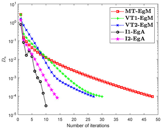
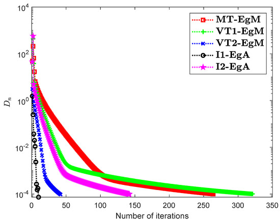
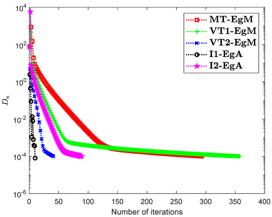
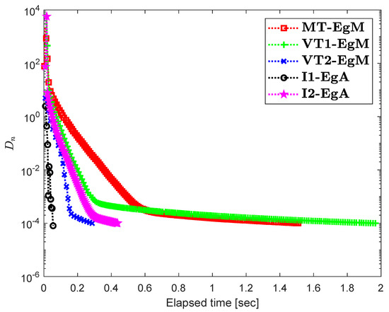
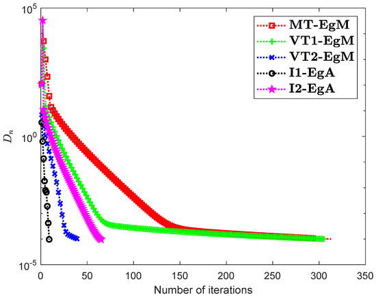
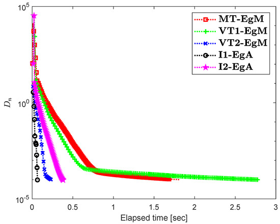
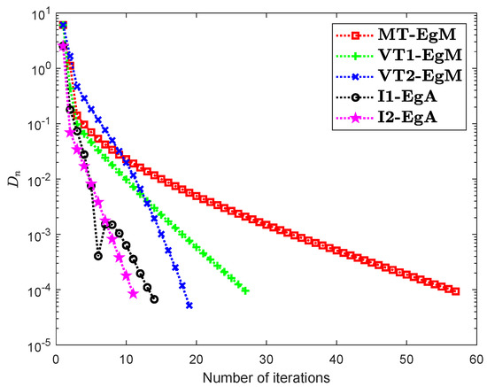
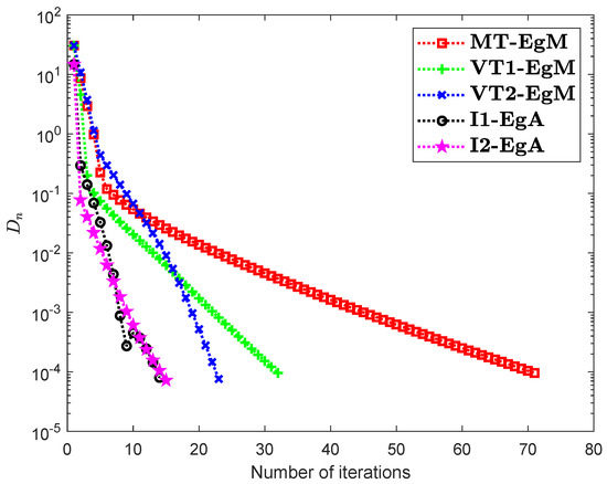
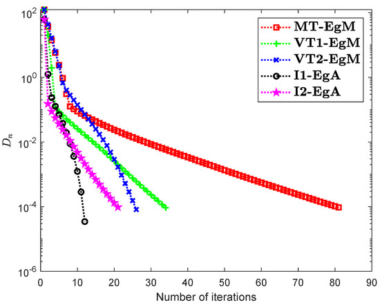
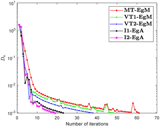
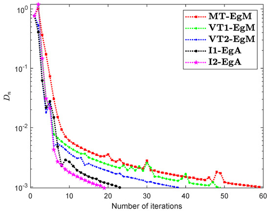
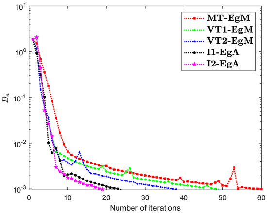
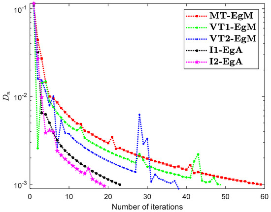
It is clear that $\mathcal{G}$ is monotone and Lipschitz continuous through $L=\parallel M\parallel .$ For $q=0$, the solution set of the corresponding variational inequality problem is $\Omega =\left\{0\right\}$. During this experiment, the initial point is $u_0=u_1=(1,1,\cdots ,1)$ and $D_n=\parallel w_n-y_n\parallel \le {10}^{-4}.$ The numerical findings of these methods are shown in Figure 1, Figure 2, Figure 3, Figure 4, Figure 5 and Figure 6 and Table 1. The control conditions are taken as follows:

Figure 1. Numerical illustration of Algorithms 1 and 2 with Algorithm 3.4 in [23] and Algorithm 3.2 in [24] and Algorithm 3.1 in [25] when $m=5.$

Figure 2. Numerical illustration of Algorithms 1 and 2 with Algorithm 3.4 in [23] and Algorithm 3.2 in [24] and Algorithm 3.1 in [25] when $m=20.$

Figure 3. Numerical illustration of Algorithms 1 and 2 with Algorithm 3.4 in [23] and Algorithm 3.2 in [24] and Algorithm 3.1 in [25] when $m=50.$

Figure 4. Numerical illustration of Algorithms 1 and 2 with Algorithm 3.4 in [23] and Algorithm 3.2 in [24] and Algorithm 3.1 in [25] when $m=50.$

Figure 5. Numerical illustration of Algorithms 1 and 2 with Algorithm 3.4 in [23] and Algorithm 3.2 in [24] and Algorithm 3.1 in [25] when $m=100.$

Figure 6. Numerical illustration of Algorithms 1 and 2 with Algorithm 3.4 in [23] and Algorithm 3.2 in [24] and Algorithm 3.1 in [25] when $m=100.$

Table 1. Numerical data for Figure 1, Figure 2, Figure 3, Figure 4, Figure 5 and Figure 6.

Dimension	$\mathit{m}=5$		$\mathit{m}=20$		$\mathit{m}=50$		$\mathit{m}=100$
Algorithm Name	Iter.	Time	Iter.	Time	Iter.	Time	Iter.	Time
Algorithm 3.4 in [23]	48	0.203351	264	1.440695	294	1.514870	313	1.817463
Algorithm 3.2 in [24]	30	0.150336	321	1.766826	357	1.966747	306	2.782575
Algorithm 3.1 in [25]	27	0.131781	42	0.182407	41	0.286670	40	0.234242
Algorithm 1	10	0.074348	10	0.041680	10	0.055002	9	0.064665
Algorithm 2	14	0.064953	142	0.672565	89	0.437610	65	0.380447

(i) 

Algorithm 3.4 in [23] (shortly, MT-EgM):

$${\chi }_0=0.20,\theta =0.70,\mu =0.30,{\varphi }_n=\frac{1}{(n+2)},{\tau }_n=\frac{1}{{(n+1)}^2},{\theta }_n=\frac{5}{10}(1-{\varphi }_n).$$

(ii) 

Algorithm 3.2 in [24] (shortly, VT1-EgM):

$${\tau }_0=0.20,\theta =0.50,\mu =0.50,{\varphi }_n=\frac{1}{(n+1)},{ϵ}_n=\frac{1}{{(n+1)}^2},f\left(u\right)=\frac{u}{3}.$$

(iii) 

Algorithm 3.1 in [25] (shortly, VT2-EgM):

$$\chi =\frac{0.7}{L},\theta =0.70,{\varphi }_n=\frac{1}{(n+2)},{\tau }_n=\frac{1}{{(n+1)}^2},f\left(u\right)=\frac{u}{3}.$$

(iv) 

Algorithm 1 (shortly, I1-EgA):

$$\chi =\frac{0.7}{L},\theta =0.70,{\varphi }_n=\frac{1}{(n+2)},{ϵ}_n=\frac{1}{{(n+1)}^2}.$$

(v) 

Algorithm 2 (shortly, I2-EgA):

$${\chi }_0=0.20,\mu =0.30,\theta =0.70,{\varphi }_n=\frac{1}{(n+2)},{ϵ}_n=\frac{1}{{(n+1)}^2}.$$

Example 2.

Assume that $\mathcal{H}=L^2\left([0,1]\right)$ is a Hilbert space with an inner product

$$⟨u,y⟩={\int }_0^{1}u\left(t\right)y\left(t\right)dt,\forall u,y\in \mathcal{H}$$

and norm is defined by

$$\parallel u\parallel =\sqrt{{\int }_0^1{\left|u\left(t\right)\right|}^{2}dt}.$$

Consider that the set $\mathcal{C}:=\{u\in L^2\left([0,1]\right):\parallel u\parallel \le 1\}$ is a unit ball. Let $\mathcal{G}:\mathcal{C}\to \mathcal{H}$ is defined by

$$\mathcal{G}\left(u\right)\left(t\right)={\int }_0^1\left(u\left(t\right)-H(t,s)f\left(u\right(s\left)\right)\right)ds+g\left(t\right)$$

where

$$H(t,s)=\frac{2ts{e}^{(t+s)}}{e\sqrt{e^2-1}},f\left(u\right)=cosu,g\left(t\right)=\frac{2t{e}^t}{e\sqrt{e^2-1}}.$$

It can be seen that $\mathcal{G}$ is Lipschitz-continuous with Lipschitz constant $L=2$ and monotone. Figure 7, Figure 8 and Figure 9 and Table 2 show the numerical results by choosing different choices of $u_0$. The control conditions are taken as follows:

Figure 7. Numerical illustration of Algorithms 1 and 2 with Algorithm 3.4 in [23] and Algorithm 3.2 in [24] and Algorithm 3.1 in [25] when $u_0=u_1=t^2+1$.

Figure 8. Numerical illustration of Algorithms 1 and 2 with Algorithm 3.4 in [23] and Algorithm 3.2 in [24] and Algorithm 3.1 in [25] when $u_0=u_1=3t^2+2sin\left(t\right)$.

Figure 9. Numerical illustration of Algorithms 1 and 2 with Algorithm 3.4 in [23] and Algorithm 3.2 in [24] and Algorithm 3.1 in [25] when $u_0=u_1=5t^2+e^t$.

Table 2. Numerical data for Figure 7, Figure 8 and Figure 9.

${\mathit{u}}_0={\mathit{u}}_1$	${\mathit{t}}^2+1$		$3{\mathit{t}}^2+2sin\left(\mathit{t}\right)$		${\mathit{t}}^2+{\mathit{e}}^{\mathit{t}}$
Algorithm Name	Iter.	Time	Iter.	Time	Iter.	Time
Algorithm 3.4 in [23]	57	0.037861	71	0.168874	81	0.207324
Algorithm 3.2 in [24]	27	0.021260	32	0.086875	34	0.109731
Algorithm 3.1 in [25]	19	0.012435	23	0.042838	26	0.049123
Algorithm 1	14	0.014493	14	0.032441	12	0.031265
Algorithm 2	11	0.017906	15	0.042816	21	0.076447

(i) 

Algorithm 3.4 in [23] (shortly, MT-EgM):

$${\chi }_0=0.25,\theta =0.75,\mu =0.35,{\tau }_n=\frac{1}{{(n+1)}^2},{\varphi }_n=\frac{1}{2(n+2)},{\theta }_n=\frac{6}{10}(1-{\varphi }_n).$$

(ii) 

Algorithm 3.2 in [24] (shortly, VT1-EgM):

$${\tau }_0=0.25,\theta =0.75,\mu =0.35,{ϵ}_n=\frac{1}{{(n+1)}^2},{\varphi }_n=\frac{1}{2(n+2)},f\left(u\right)=\frac{u}{4}.$$

(iii) 

Algorithm 3.1 in [25] (shortly, VT2-EgM):

$$\chi =\frac{0.75}{L},\theta =0.75,{\tau }_n=\frac{1}{{(n+1)}^2},{\varphi }_n=\frac{1}{2(n+2)},f\left(u\right)=\frac{u}{4}.$$

(iv) 

Algorithm 1 (shortly, I1-EgA):

$$\chi =\frac{0.75}{L},\theta =0.75,{ϵ}_n=\frac{1}{{(n+1)}^2},{\varphi }_n=\frac{1}{2(n+2)}.$$

(v) 

Algorithm 2 (shortly, I2-EgA):

$${\chi }_0=0.25,\mu =0.35,\theta =0.75,{ϵ}_n=\frac{1}{{(n+1)}^2},{\varphi }_n=\frac{1}{2(n+2)}.$$

Example 3.

Consider that the problem of Kojima–Shindo where the constraint set $\mathcal{C}$ is

$$\mathcal{C}=\{u\in {\mathbb{R}}^4:1\le u_i\le 5,i=1,2,3,4\},$$

and the mapping $\mathcal{G}:{\mathbb{R}}^4\to {\mathbb{R}}^4$ is defined by

$$\begin{array}{c}\hfill \mathcal{G}\left(u\right)=\left(\begin{array}{c}{u}_1+u_2+u_3+u_4-4u_2{u}_3{u}_4\\ u_1+u_2+u_3+u_4-4u_1{u}_3{u}_4\\ u_1+u_2+u_3+u_4-4u_1{u}_2{u}_4\\ u_1+u_2+u_3+u_4-4u_1{u}_2{u}_3\end{array}\right).\end{array}$$

It is easy to see that $\mathcal{G}$ is not monotone on the set $\mathcal{C}.$ By using the Monte-Carlo approach [34], it can be shown that $\mathcal{G}$ is pseudo-monotone on $\mathcal{C}.$ This problem has a unique solution $u^{*}={(5,5,5,5)}^T.$ Actually, in general, it is a very difficult task to check the pseudomonotonicity of any mapping $\mathcal{G}$ in practice. We here employ the Monte Carlo approach according to the definition of pseudo-monotonicity: Generate a large number of pairs of points u and y uniformly in $\mathcal{C}$ satisfying $\mathcal{G}{\left(u\right)}^T(y-u)\ge 0$ and then check if $\mathcal{G}{\left(y\right)}^T(y-u)\ge 0$. Table 3, Table 4, Table 5, Table 6, Table 7 and Table 8 show the numerical results by taking different values of $u_0$. The control conditions are taken as follows:

Table 3. Example 3: Numerical findings of Algorithm 3.4 in [23] and $u_0=u_1={(1,2,3,4)}^T$.

Iter (n)	${\mathit{u}}_1$	${\mathit{u}}_2$	${\mathit{u}}_3$	${\mathit{u}}_4$
1	7.88110105259549	11.1335921052147	11.6608026315329	11.4916973684078
2	2.72517069971347	5.52196307009909	5.91062617486984	5.78231681677249
3	2.74650358169779	5.23892462205654	5.43540972965547	5.37058363048288
4	2.79589652551700	5.10560097798145	5.20481731038818	5.17209179402342
5	2.84815300477526	5.04321208318383	5.09330195427214	5.07678246381620
6	2.90242325540275	5.01444727730850	5.03972755805987	5.03139070422338
7	2.95876979857588	5.00154113107122	5.01429541422714	5.01008946137975
8	3.01614532087206	4.99604650580771	5.00248193413128	5.00035976548024
⋮	⋮	⋮	⋮	⋮
194	4.99949159554096	4.99949159554096	4.99949159554096	4.99949159554096
195	4.99949420145518	4.99949420145518	4.99949420145518	4.99949420145518
196	4.99949678078979	4.99949678078979	4.99949678078979	4.99949678078979
197	4.99949933394941	4.99949933394941	4.99949933394941	4.99949933394941
198	4.99950186133047	4.99950186133047	4.99950186133047	4.99950186133047
CPU time is seconds	1.011633

Table 4. Example 3: Numerical findings of Algorithm 3.2 in [24] and $u_0=u_1={(1,2,3,4)}^T$.

Iter (n)	${\mathit{u}}_1$	${\mathit{u}}_2$	${\mathit{u}}_3$	${\mathit{u}}_4$
1	4.94814814707507	20.1659074073104	20.2289444443514	18.9075370362809
2	−8.04670389554580	12.4597307883609	12.5054021946827	11.3787988702116
3	1.03972935440247	4.90132095088790	4.89452802770933	4.98533018397129
4	1.11973537635742	4.89218078676053	4.88537889965809	4.95475431398367
5	1.20128523014071	4.89169908830941	4.88493057181313	4.94635475329384
6	1.27774539110779	4.89625929375273	4.88953484996449	4.94790178020963
7	1.34983811312425	4.90378394656115	4.89710336213719	4.95376528318611
8	1.41896397454886	4.91334870977828	4.90670981629961	4.96199173340817
⋮	⋮	⋮	⋮	⋮
144	4.99948911782781	4.99948911782781	4.99948911782781	4.99948911782781
145	4.99949261719944	4.99949261719944	4.99949261719944	4.99949261719944
146	4.99949606895811	4.99949606895811	4.99949606895811	4.99949606895811
147	4.99949947406902	4.99949947406902	4.99949947406902	4.99949947406902
148	4.99950283347142	4.99950283347142	4.99950283347142	4.99950283347142
CPU time is seconds	0.7115419

Table 5. Example 3: Numerical findings of Algorithm 2 and $u_0=u_1={(1,2,3,4)}^T$.

Iter (n)	${\mathit{u}}_1$	${\mathit{u}}_2$	${\mathit{u}}_3$	${\mathit{u}}_4$
1	4.99999999934819	20.0658752056891	20.0955845156778	18.7728355231621
2	−7.83144812920198	11.9265613339038	11.9437095513756	10.8524606746456
3	1.01490159056644	4.96724347328928	4.96512000980275	5.10532223071200
4	1.10642915068494	4.93819144878954	4.93599467724991	4.99999999995773
5	1.18463430195965	4.93374030970576	4.93153342235750	4.97372522603788
6	1.26412238398338	4.93785658351241	4.93565678779788	4.96968839262467
7	1.33805311564430	4.94627563468593	4.94408827533979	4.97519539293950
8	1.40748289276225	4.95692798081047	4.95475304777657	4.98440717807182
⋮	⋮	⋮	⋮	⋮
96	4.99999999962290	4.99999999962290	4.99999999962290	4.99999999962290
97	4.99999999962318	4.99999999962318	4.99999999962318	4.99999999962318
98	4.99999999962346	4.99999999962346	4.99999999962346	4.99999999962346
99	4.99999999962373	4.99999999962373	4.99999999962373	4.99999999962373
100	4.99999999962399	4.99999999962399	4.99999999962399	4.99999999962399
CPU time is seconds	0.503420

Table 6. Example 3: Numerical findings of Algorithm 3.4 in [23] and $u_0=u_1={(-1,0,1,2)}^T$.

Iter (n)	${\mathit{u}}_1$	${\mathit{u}}_2$	${\mathit{u}}_3$	${\mathit{u}}_4$
1	0.116881581449987	0.813197370923916	1.11161842825326	1.96709210640194
2	0.544096187738739	0.963936802772123	1.15066880224072	1.94902465158251
3	0.767743928389032	1.01063135569287	1.17422202753691	1.93884243796376
4	0.883925792457061	1.04508825238764	1.19706742465652	1.93285090332439
5	0.943732024663154	1.07700290591513	1.21999679143733	1.92972670723471
6	0.985076884925896	1.10717191339312	1.24263089418537	1.92912929557214
7	1.02327142457484	1.13769463060810	1.26640373232346	1.93117221434202
8	1.06041942145622	1.16848656060979	1.29115424126752	1.93571856968895
⋮	⋮	⋮	⋮	⋮
178	4.99949304114715	4.99949304114715	4.99949304114715	4.99949304114715
179	4.99949586970068	4.99949586970068	4.99949586970068	4.99949586970068
180	4.99949866686358	4.99949866686358	4.99949866686358	4.99949866686358
181	4.99950143315555	4.99950143315555	4.99950143315555	4.99950143315555
182	4.99950416908485	4.99950416908485	4.99950416908485	4.99950416908485
CPU time is seconds	0.957781

Table 7. Example 3: Numerical findings of Algorithm 3.2 in [24] and $u_0=u_1={(-1,0,1,2)}^T$.

Iter (n)	${\mathit{u}}_1$	${\mathit{u}}_2$	${\mathit{u}}_3$	${\mathit{u}}_4$
1	0.760053582775300	1.29003298382748	1.20319480217964	1.94068518744861
2	1.21804298615978	1.59414241359208	1.42464988939697	2.01820655416591
3	1.42659480361034	1.73943108707035	1.57161284553192	2.09415611599989
4	1.57886167340713	1.85447528443790	1.69967500052918	2.17426416753376
5	1.71808153256788	1.96701984456950	1.82539532502208	2.26236423411214
6	1.85632702927712	2.08392415770031	1.95375834077497	2.35895786218053
7	1.99842296843380	2.20786382779888	2.08766201331954	2.46482556588447
8	2.14689895343515	2.34039691864025	2.22903433081793	2.58085673886984
⋮	⋮	⋮	⋮	⋮
144	4.99948910579703	4.99948910579703	4.99948910579703	4.99948910579703
145	4.99949260517052	4.99949260517052	4.99949260517052	4.99949260517052
146	4.99949605693103	4.99949605693103	4.99949605693103	4.99949605693103
147	4.99949946204375	4.99949946204375	4.99949946204375	4.99949946204375
148	4.99950282144794	4.99950282144794	4.99950282144794	4.99950282144794
CPU time is seconds	0.8748252

Table 8. Example 3: Numerical findings of Algorithm 2 and $u_0=u_1={(-1,0,1,2)}^T$.

Iter (n)	${\mathit{u}}_1$	${\mathit{u}}_2$	${\mathit{u}}_3$	${\mathit{u}}_4$
1	0.775171247844478	1.30058646543549	1.21022901009941	1.94547500162994
2	1.21446821311615	1.59315820520707	1.41802847051195	2.01854575677085
3	1.40930154934255	1.72830536082867	1.55238769919704	2.08704132135424
4	1.55005042100928	1.83358202294312	1.66945202714427	2.15901099064876
5	1.67652335037437	1.93461531040966	1.78314662252036	2.23718181897121
6	1.80020428317844	2.03794015805606	1.89767214585452	2.32166725738566
7	1.92573577123647	2.14610904279505	2.01564105118587	2.41306525933486
8	2.05546783590764	2.26053026824905	2.13879627759795	2.51211478239818
⋮	⋮	⋮	⋮	⋮
96	4.99999999998368	4.99999999998368	4.99999999998368	4.99999999998368
97	4.99999999998368	4.99999999998368	4.99999999998368	4.99999999998368
98	4.99999999998368	4.99999999998368	4.99999999998368	4.99999999998368
99	4.99999999998369	4.99999999998369	4.99999999998369	4.99999999998369
100	4.99999999998369	4.99999999998369	4.99999999998369	4.99999999998369
CPU time is seconds	0.544268

(i) 

Algorithm 3.4 in [23] (shortly, MT-EgM):

$${\chi }_0=0.05,\theta =0.70,\mu =0.33,{\tau }_n=\frac{1}{{(n+1)}^2},{\varphi }_n=\frac{1}{50(n+2)},{\theta }_n=\frac{6}{10}(1-{\varphi }_n).$$

(ii) 

Algorithm 3.2 in [24] (shortly, VT1-EgM):

$${\tau }_0=0.05,\theta =0.70,\mu =0.33,{ϵ}_n=\frac{1}{{(n+1)}^2},{\varphi }_n=\frac{1}{50(n+2)},f\left(u\right)=\frac{u}{3}.$$

(iii) 

Algorithm 3.1 in [25] (shortly, VT2-EgM):

$$\chi =\frac{0.7}{L},\theta =0.70,{\tau }_n=\frac{1}{{(n+1)}^2},{\varphi }_n=\frac{1}{50(n+2)},f\left(u\right)=\frac{u}{3}.$$

(iv) 

Algorithm 1 (shortly, I1-EgA):

$$\chi =\frac{0.7}{L},\theta =0.70,{ϵ}_n=\frac{1}{{(n+1)}^2},{\varphi }_n=\frac{1}{50(n+2)}.$$

(v) 

Algorithm 2 (shortly, I2-EgA):

$${\chi }_0=0.05,\mu =0.33,\theta =0.70,{ϵ}_n=\frac{1}{{(n+1)}^2},{\varphi }_n=\frac{1}{50(n+2)}.$$

Example 4.

The last Example has taken from [35] where $\mathcal{G}:{\mathbb{R}}^2\to {\mathbb{R}}^2$ is defined by

$$\mathcal{G}\left(u\right)=\left(\begin{array}{c}0.5u_1{u}_2-2u_2-{10}^7\\ -4u_1-0.1u_2^2-{10}^7\end{array}\right)$$

where $\mathcal{C}=\{u\in {\mathbb{R}}^2:{(u_1-2)}^2+{(u_2-2)}^2\le 1\}.$ It can easily see that $\mathcal{G}$ is Lipschitz continuous with $L=5$ and $\mathcal{G}$ is not monotone on $\mathcal{C}$ but pseudomonotone. Here, the above problem has unique solution $u^{*}={(2.707,2.707)}^T.$ Figure 10, Figure 11, Figure 12 and Figure 13 and Table 9 show the numerical findings by letting different values of $u_0$. The control conditions are taken as follows:

Figure 10. Numerical illustration of Algorithms 1 and 2 with Algorithm 3.4 in [23] and Algorithm 3.2 in [24] and Algorithm 3.1 in [25] when $u_0=u_1={(1.5,1.7)}^T$.

Figure 11. Numerical illustration of Algorithms 1 and 2 with Algorithm 3.4 in [23] and Algorithm 3.2 in [24] and Algorithm 3.1 in [25] when $u_0=u_1={(2.0,3.0)}^T$.

Figure 12. Numerical illustration of Algorithms 1 and 2 with Algorithm 3.4 in [23] and Algorithm 3.2 in [24] and Algorithm 3.1 in [25] when $u_0=u_1={(1.0,2.0)}^T$.

Figure 13. Numerical illustration of Algorithms 1 and 2 with Algorithm 3.4 in [23] and Algorithm 3.2 in [24] and Algorithm 3.1 in [25] when $u_0=u_1={(2.7,2.6)}^T$.

Table 9. Numerical data for Figure 7, Figure 8 and Figure 9.

${\mathit{u}}_0={\mathit{u}}_1$	${(1.5,1.7)}^{\mathit{T}}$		${(2.0,3.0)}^{\mathit{T}}$		${(1.0,2.0)}^{\mathit{T}}$		${(2.7,2.6)}^{\mathit{T}}$
Algorithm Name	Iter.	Time	Iter.	Time	Iter.	Time	Iter.	Time
Algorithm 3.4 in [23]	61	3.083492	59	4.127714	60	2.882394	59	3.111729
Algorithm 3.2 in [24]	48	2.189625	49	2.674055	49	2.448063	49	2.306584
Algorithm 3.1 in [25]	38	1.440188	38	1.684040	38	1.784568	38	1.645227
Algorithm 1	23	0.933457	23	1.021092	24	1.139583	23	0.922199
Algorithm 2	19	0.899018	19	0.969045	19	0.907344	19	0.953694

(i) 

Algorithm 3.4 in [23] (shortly, MT-EgM):

$${\chi }_0=0.35,\theta =0.80,\mu =0.55,{\tau }_n=\frac{1}{{(n+1)}^2},{\varphi }_n=\frac{1}{100(n+2)},{\theta }_n=\frac{6}{10}(1-{\varphi }_n).$$

(ii) 

Algorithm 3.2 in [24] (shortly, VT1-EgM):

$${\tau }_0=0.35,\theta =0.80,\mu =0.55,{ϵ}_n=\frac{1}{{(n+1)}^2},{\varphi }_n=\frac{1}{100(n+1)},f\left(u\right)=\frac{u}{5}.$$

(iii) 

Algorithm 3.1 in [25] (shortly, VT2-EgM):

$$\chi =\frac{0.8}{L},\theta =0.80,{\tau }_n=\frac{1}{{(n+1)}^2},{\varphi }_n=\frac{1}{100(n+2)},f\left(u\right)=\frac{u}{5}.$$

(iv) 

Algorithm 1 (shortly, I1-EgA):

$$\chi =\frac{0.8}{L},\theta =0.80,{ϵ}_n=\frac{1}{{(n+1)}^2},{\varphi }_n=\frac{1}{100(n+2)}.$$

(v) 

Algorithm 2 (shortly, I2-EgA):

$${\chi }_0=0.35,\mu =0.55,\theta =0.80,{ϵ}_n=\frac{1}{{(n+1)}^2},{\varphi }_n=\frac{1}{100(n+2)}.$$

5. Conclusions

In this study, we have introduced two new methods for finding a solution of variational inequality problem in a Hilbert space. The results have been established on the base of two previous methods: the subgradient extragradient method and the inertial method. Some new approaches to the inertial framework and the step size rule have been set up. The strong convergence of our proposed methods is set up under the condition of pseudo-monotonicity and Lipschitz continuity of mapping. Some numerical results are presented to explain the convergence of the methods over others. The results in this paper have been used as methods for figuring out the variational inequality problem in Hilbert spaces. Finally, numerical experiments indicate that the inertial approach normally enhances the performance of the proposed methods.

References

- Konnov, I.V. On systems of variational inequalities. Russ. Math. C/C Izv. Vyss. Uchebnye Zaved. Mat. 1997, 41, 77–86. [Google Scholar]
- Stampacchia, G. Formes bilinéaires coercitives sur les ensembles convexes. Comptes Rendus Hebd. Seances Acad. Sci. 1964, 258, 4413. [Google Scholar]
- Elliott, C.M. Variational and quasivariational inequalities applications to free—boundary ProbLems. (claudio baiocchi and antónio capelo). SIAM Rev. 1987, 29, 314–315. [Google Scholar] [CrossRef]
- Kassay, G.; Kolumbán, J.; Páles, Z. On nash stationary points. Publ. Math. 1999, 54, 267–279. [Google Scholar]
- Kassay, G.; Kolumbán, J.; Páles, Z. Factorization of minty and stampacchia variational inequality systems. Eur. J. Oper. Res. 2002, 143, 377–389. [Google Scholar] [CrossRef]
- Kinderlehrer, D.; Stampacchia, G. An Introduction to Variational Inequalities and Their Applications; Society for Industrial and Applied Mathematics: Philadelphia, PA, USA, 2000. [Google Scholar]
- Konnov, I. Equilibrium Models and Variational Inequalities; Elsevier: Amsterdam, The Netherlands, 2007; Volume 210. [Google Scholar]
- Nagurney, A.; Economics, E.N. A Variational Inequality Approach; Springer: Boston, MA, USA, 1999. [Google Scholar]
- Takahashi, W. Introduction to Nonlinear and Convex Analysis; Yokohama Publishers: Yokohama, Japan, 2009. [Google Scholar]
- Censor, Y.; Gibali, A.; Reich, S. The subgradient extragradient method for solving variational inequalities in Hilbert space. J. Optim. Theory Appl. 2010, 148, 318–335. [Google Scholar] [CrossRef] [PubMed]
- Censor, Y.; Gibali, A.; Reich, S. Extensions of korpelevich extragradient method for the variational inequality problem in euclidean space. Optimization 2012, 61, 1119–1132. [Google Scholar] [CrossRef]
- Iusem, A.N.; Svaiter, B.F. A variant of korpelevich’s method for variational inequalities with a new search strategy. Optimization 1997, 42, 309–321. [Google Scholar] [CrossRef]
- Korpelevich, G. The extragradient method for finding saddle points and other problems. Matecon 1976, 12, 747–756. [Google Scholar]
- Malitsky, Y.V.; Semenov, V.V. An extragradient algorithm for monotone variational inequalities. Cybern. Syst. Anal. 2014, 50, 271–277. [Google Scholar] [CrossRef]
- Moudafi, A. Viscosity approximation methods for fixed-points problems. J. Math. Anal. Appl. 2000, 241, 46–55. [Google Scholar] [CrossRef]
- Noor, M.A. Some iterative methods for nonconvex variational inequalities. Comput. Math. Model. 2010, 21, 97–108. [Google Scholar] [CrossRef]
- Thong, D.V.; Hieu, D.V. Modified subgradient extragradient method for variational inequality problems. Numer. Algorithms 2017, 79, 597–610. [Google Scholar] [CrossRef]
- Thong, D.V.; Hieu, D.V. Weak and strong convergence theorems for variational inequality problems. Numer. Algorithms 2017, 78, 1045–1060. [Google Scholar] [CrossRef]
- Tseng, P. A modified forward-backward splitting method for maximal monotone mappings. SIAM J. Control Optim. 2000, 38, 431–446. [Google Scholar] [CrossRef]
- Zhang, L.; Fang, C.; Chen, S. An inertial subgradient-type method for solving single-valued variational inequalities and fixed point problems. Numer. Algorithms 2018, 79, 941–956. [Google Scholar] [CrossRef]
- Antipin, A.S. On a method for convex programs using a symmetrical modification of the lagrange function. Ekon. Mat. Metod. 1976, 12, 1164–1173. [Google Scholar]
- Polyak, B. Some methods of speeding up the convergence of iteration methods. USSR Comput. Math. Math. Phys. 1964, 4, 1–17. [Google Scholar] [CrossRef]
- Anh, P.K.; Thong, D.V.; Vinh, N.T. Improved inertial extragradient methods for solving pseudo-monotone variational inequalities. Optimization 2020, 1–24. [Google Scholar] [CrossRef]
- Thong, D.V.; Hieu, D.V.; Rassias, T.M. Self adaptive inertial subgradient extragradient algorithms for solving pseudomonotone variational inequality problems. Optim. Lett. 2019, 14, 115–144. [Google Scholar] [CrossRef]
- Thong, D.V.; Vinh, N.T.; Cho, Y.J. A strong convergence theorem for tseng’s extragradient method for solving variational inequality problems. Optim. Lett. 2019, 14, 1157–1175. [Google Scholar] [CrossRef]
- Bauschke, H.H.; Combettes, P.L. Convex Analysis and Monotone Operator Theory in Hilbert Spaces; Springer: Berlin/Heidelberg, Germany, 2011; Volume 408. [Google Scholar]
- Xu, H.-K. Another control condition in an iterative method for nonexpansive mappings. Bull. Aust. Math. Soc. 2002, 65, 109–113. [Google Scholar] [CrossRef]
- Maingé, P.-E. Strong convergence of projected subgradient methods for nonsmooth and nonstrictly convex minimization. Set-Valued Anal. 2008, 16, 899–912. [Google Scholar] [CrossRef]
- Takahashi, W. Nonlinear Functional Analysis; Yokohama Publishers: Yokohama, Japan, 2000. [Google Scholar]
- Harker, P.T.; Pang, J.-S. For the linear complementarity problem. Comput. Solut. Nonlinear Syst. Equ. 1990, 26, 265. [Google Scholar]
- Dong, Q.L.; Cho, Y.J.; Zhong, L.L.; Rassias, T.M. Inertial projection and contraction algorithms for variational inequalities. J. Glob. Optim. 2017, 70, 687–704. [Google Scholar] [CrossRef]
- Hieu, D.V.; Anh, P.K.; Muu, L.D. Modified hybrid projection methods for finding common solutions to variational inequality problems. Comput. Optim. Appl. 2016, 66, 75–96. [Google Scholar] [CrossRef]
- Solodov, M.V.; Svaiter, B.F. A new projection method for variational inequality problems. SIAM J. Control Optim. 1999, 37, 765–776. [Google Scholar] [CrossRef]
- Hu, X.; Wang, J. Solving pseudomonotone variational inequalities and pseudoconvex optimization problems using the projection neural network. IEEE Trans. Neural Netw. 2006, 17, 1487–1499. [Google Scholar]
- Shehu, Y.; Dong, Q.-L.; Jiang, D. Single projection method for pseudo-monotone variational inequality in Hilbert spaces. Optimization 2018, 68, 385–409. [Google Scholar] [CrossRef]
Publisher’s Note: MDPI stays neutral with regard to jurisdictional claims in published maps and institutional affiliations. |
© 2021 by the authors. Licensee MDPI, Basel, Switzerland. This article is an open access article distributed under the terms and conditions of the Creative Commons Attribution (CC BY) license (http://creativecommons.org/licenses/by/4.0/).