Fuzzy Interpolation with Extensional Fuzzy Numbers

Abstract

The article develops further directions stemming from the arithmetic of extensional fuzzy numbers. It presents the existing knowledge of the relationship between the arithmetic and the proposed orderings of extensional fuzzy numbers—so-called $\mathcal{S}$-orderings—and investigates distinct properties of such orderings. The desirable investigation of the $\mathcal{S}$-orderings of extensional fuzzy numbers is directly used in the concept of $\mathcal{S}$-function—a natural extension of the notion of a function that, in its arguments as well as results, uses extensional fuzzy numbers. One of the immediate subsequent applications is fuzzy interpolation. The article provides readers with the basic fuzzy interpolation method, investigation of its properties and an illustrative experimental example on real data. The goal of the paper is, however, much deeper than presenting a single fuzzy interpolation method. It determines direction to a wide variety of fuzzy interpolation as well as other analytical methods stemming from the concept of $\mathcal{S}$-function and from the arithmetic of extensional fuzzy numbers in general.

1. Introduction

Fuzzy interpolation is a generally well-established area with crucial results. Indeed, it is a natural area that has a deep connection to distinct areas. We can consider, e.g., the interpolation of fuzzy rule bases with logical motivations stemming from approximate reasoning where the pairs of antecedent and consequent fuzzy sets of a fuzzy rule base establish “pairs of fuzzy points” and the task is to infer an appropriate output fuzzy set for an input fuzzy sets lying in between of the antecedents. In this logical setting, such an interpolation task leads to the solvability of fuzzy relational equations—an area initiated by Sanchez [1] and followed by many others, see [2,3,4,5]. The interest of the community in this area does not seem to disappear [1] as it moves to the investigation of distinct extensions [6,7,8].

Another direction of fuzzy interpolation was rather geometrically motivated although the connection to fuzzy rule-based systems was declared too. The geometrical approaches often stem from usual interpolations (linear [9] or spline [10]) extended to fuzzy numbers and allow the interpolation of sparse rule bases [11,12]. Due to the importance of the interpolation for the approximate reasoning, decision-making or optimization, we may observe the interest of the community into this direction too [13]. For the comparison of some fundamentals, we refer readers to [14] and we also highlight a work that up to some degree combines both approaches and serves us one of our motivations [15].

Our work follows this attempt of joining both views. It works with pairs of fuzzy numbers representing ague quantities [16] and interpolates even a sparse case. However, the fuzzy numbers as well as the manipulation with them will be deeply stemming from fuzzy relational calculus [17], similarity relations, extensional hulls and other concepts related to the approximate reasoning [18].

In particular, we will deal with the MI-algebra-based arithmetics based on extensional fuzzy numbers, i.e., extensional hulls of crisp numbers constructed with respect to some similarity relations [19]. Such arithmetic serves as an alternative to other technical approaches [20,21] allowing the formalization of the ideas of Mareš [22] in a way that splits the often time-consuming process of calculating operations on fuzzy numbers into a two-step procedure: one calculating the standard operation on crisp points, the other one on processing the similarity relations forming fuzzy numbers around the crisp points. Indeed, as the extensional fuzzy numbers are nothing else but extensional hulls of crisp numbers, we get genuine representations of vague quantities—collections of points similar to the given crisp point. And operations on such objects, e.g., when summing up “about 3” and “about 5”, are intuitively performed by a human brain by adding the crisp numbers 3 and 5 to a partial result 8 which is later viewed with a tolerance measure respecting that both entries were imprecise. This tolerance measure is nothing else but a similarity relation that is a result of the operation on similarities used in the construction of both extensional fuzzy numbers.

The difference in the used arithmetic, of course, also changes the interpolation method and its results. Any classical interpolation can be extended to a fuzzy interpolation method, assuming that the used arithmetic is functional and equipped with all the necessary operations. Apart from the arithmetical operations, also other fundamental mathematical concepts, such as ordering of fuzzy numbers, must be developed. Thus, we adopt the orderings of extensional fuzzy numbers introduced in [23] and studied in [24]. It is important to note that such an ordering is tightly connected to the arithmetic itself, which we find essential.

The structure of the article is as follows. Section 2 recalls the basic preliminaries about the arithmetics of extensional fuzzy numbers. Section 3 recalls the approach to the orderings of extensional fuzzy numbers and Section 4 sets up their crucial properties. Section 5 leads the investigation towards fuzzy interpolation that is, later, in Section 6 experimentally demonstrated on an illustrative example from the real practice. Section 7 closes the article with a brief discussion.

2. Preliminaries—Arithmetical Operations on Extensional Fuzzy Numbers

2.1. Motivation and the Main Concepts

The arithmetic of extensional fuzzy numbers has been originally proposed in [25,26] as an alternative to other functional arithmetics that are often stemming from Zadeh’s extension principle. Such arithmetics often consider the $\alpha$-cut calculus and they are more technically oriented based on distinct parametric representations of fuzzy numbers [21,27,28].

The proposed alternative (detail description in [19]), was motivated from the non-preservation of some algebraic properties by the existing approaches, especially the non-existence of inverse elements. This is nothing surprising as the models of vague quantities provided by fuzzy numbers are rather fuzzy intervals than fuzzy numbers, and the absence of an inverse element is a feature of the interval calculus, see [29]. However, as pointed out by Mareš [16], instead of considering only a single crisp neutral element, we may observe infinitely many “neutral-like” elements so, when solving equations with vague quantities, we get the equality of both sides up to “nearly zero”. Therefore, there is no absence of the inverse, the operations on inverses only do not lead to the genuine neutral (identity) element but to any of the identity-like elements. This idea of Mareš is then developed in [19] and it leads to the MI-algebras (MI stands for many identities). Algebraically, it drops the standard field structure of real numbers $(\mathbb{R},+,·)$ however, it does not harm its ideas, just incorporates them with a certain vagueness.

Above-recalled alternative approach [29] correctly stems from the fact that the lack of the preserved algebraic properties is caused by the interval character of fuzzy numbers and the non-preservation inherited from interval calculus, is “healed” by using the concept of gradual numbers that are conceptually sort of inverse to the usual fuzzy numbers (intervals). Indeed, a gradual fuzzy number $\tilde{a}$ is a mapping from the interval $(0,1]$ to the real line and the (crisp) real number a is its special case such that $\tilde{a}\left(\alpha \right)=a$ for arbitrary $\alpha \in (0,1]$. Then the arithmetic operating on such functions preserves the algebraic properties such as existence of an inverse to any element. Note that the concept is so general that it does not assume any restriction on the “shape” (e.g., on monotonicity or continuity) which is, on one hand, an advantage, on the other hand, it allows dealing with or obtaining functions hardly interpreting any vaguely given quantity.

The arithmetic of extensional fuzzy numbers stemmed from a natural model of a vague quantity and formalized human-style calculus with them. It models a vaguely given quantity “about a” as an extensional hull of the crisp value (singleton) a with respect to a given similarity relation. Thus, it has a genuine construction determining a fuzzy set of values similar to a. On one hand, as we stated, it is a fuzzy set of elements so, it leads to a set-like concept that will never possess the arithmetical properties of numbers however, it was not constructed as an (fuzzy) interval and the generating crisp number $a\in \mathbb{R}$ is available for further purposes including the calculus.

The price we pay for such a restriction to extensional hulls of crisp numbers is not high as we do not see other than technical reasons stemming from the usual arithmetics themselves (e.g., results of limits) to consider technical definitions allowing dealing with e.g., upper semi-continuous fuzzy sets as models of fuzzy numbers. In our opinion, the restriction pays off in the subsequent advantages.

Let us fix the notation for a set of fuzzy sets defined on a universe X: $\mathcal{F}\left(X\right)=\{A\mid A:X\to [0,1\left]\right\}$; and of the support of a fuzzy set A: $\mathrm{Supp}\left(A\right)=\{x\in \mathbb{R}\mid A(x)>0\}$. Now, we recall the well-known fundamental definitions adopted to the universe of real numbers.

Definition 1.

[30,31] Let ⊗ be a left-continuous t-norm. A binary fuzzy relation $S\in \mathcal{F}\left(X\right)$ is called ⊗-similarity if the following holds

(i) 

$S(x,x)=1\left(reflexivity\right)$

(ii) 

$S(x,y)=S(y,x)\left(symmetry\right)$

(iii) 

$S(x,y)\otimes S(y,z)\le S(x,z)(\otimes -transitive)$

for all $x,y,z\in \mathbb{R}$.

Definition 2.

[19] Let S be a ⊗-similarity relation. It is called separable if $S(x,y)=1$ implies that $x=y$.

Definition 3.

[19] Let S be a ⊗-similarity relation. It is called shift-invariant if $S(x,y)=S(x+z,x+z)$ for any $x,y,z\in \mathbb{R}$.

Convention 1.

Due to the practical importance of the separability property, we assume that all ⊗-similarity relations considered in this paper are separable.

Definition 4.

[30] A fuzzy set $A\in \mathcal{F}\left(\mathbb{R}\right)$ is called extensional regarding a ⊗-similarity relation S if the following holds:

$$A\left(x\right)\otimes S(x,y)\le A\left(y\right),x,y\in \mathbb{R}.$$

Example 1.

Binary fuzzy relations on $\mathbb{R}$ given by

$$S_p(x,y)=(1-p|x-y\left|\right)\vee 0,p>0$$

(1)

are the shift-invariant ⊗-similarity relations where ⊗ is the ukasiewicz t-norm.

Example 2.

Binary fuzzy relations on $\mathbb{R}$ given by

$$S_p(x,y)=e^{-p|x-y|},p>0$$

(2)

are the shift-invariant ⊗-similarity relations where ⊗ is the product t-norm.

Remark 1.

The shift-invariance is a useful property for connecting similarities and arithmetics, see Proposition 6. An example of similarity relation that is not shift-invariant can be found in Remark 2.2 in [19].

An extensional hull of a fuzzy set A is the least fuzzy superset of A that is extensional.

Theorem 1.

[31] Let S be a ⊗-similarity relation and let $A\in \mathcal{F}\left(\mathbb{R}\right)$. The extensional hull of A, denoted by $\mathrm{EXT}\left(A\right)\in \mathcal{F}\left(\mathbb{R}\right)$, is given by

$${\mathrm{EXT}}_S\left(A\right)\left(x\right)=\underset{y\in \mathbb{R}}{\bigvee }\left(A\left(y\right)\otimes S(x,y)\right).$$

(3)

If we consider a singleton representation of a real number $a\in \mathbb{R}$ that is a fuzzy set $\tilde{a}\in \mathcal{F}\left(\mathbb{R}\right)$ such that $\tilde{a}\left(a\right)=1$, and $\tilde{a}\left(x\right)=0$ for any $x\ne a$ we can construct an extensional hull of a real number. Such an object is called extensional fuzzy number or a fuzzy point, see [18,31,32].

Definition 5.

[19,25] Let $a\in \mathbb{R}$ and let S be a ⊗-similarity. Then $a_S\in \mathcal{F}\left(\mathbb{R}\right)$ given as follows:

$$a_S\left(x\right)={\mathrm{EXT}}_S\left(a\right)\left(x\right)$$

(4)

is called extensional fuzzy number.

A correct version of Formula (4) would consider the extensional hull of the singleton ${\mathrm{EXT}}_S\left(\tilde{a}\right)\left(x\right)$ but as there is no danger of confusion, we will neglect the difference between a and $\tilde{a}$ and stick to the simpler denotation. The extensional fuzzy number may be easily calculated by a simple substitution.

Lemma 1.

[19] Let $a\in \mathbb{R}$ and let S be a ⊗-similarity. Then $a_S\left(x\right)=S(a,x)$, for any $y\in \mathbb{R}$.

Convention 2.

We restrict our choice of similarities to those ensuring that the fuzzy numbers $a_S$ are formed by $\alpha$-cuts ${\left(a_S\right)}_{\alpha }$ that are closed intervals in $\mathbb{R}$.

2.2. Arithmetic of Extensional Fuzzy Numbers

The construction as well as the denotation of the extensional fuzzy number emphasizes its semantics—number a with close numbers around it—where the closeness is determined by similarity S. Such a restriction to a subclass of fuzzy numbers is reasonable and justified by the most natural representation of a vague quantity reflecting the semantics already in its construction. Furthermore, the construction allows the derivation of appropriate models of the arithmetic [25,26]—algebraically leading to MI-algebraic structures. We avoid going into algebraic details and only refer interested readers to the relevant sources, mainly to [19] and furthermore, to [33,34] for the quotient MI-groups, and to [35] for the topological MI-groups. Here, we continue only with the computational part of the arithmetic of extensional fuzzy numbers.

Consider a system of nested ⊗-similarities $\mathcal{S}$ with the bottom element ${\perp }_{\mathcal{S}}$ and the set of all fuzzy numbers that are extensional with respect to a similarity from the given system:

$${\mathcal{F}}_{\mathcal{S}}\left(\mathbb{R}\right)=\{a_S\mid a\in \mathbb{R} \mathrm{and} S\in \mathcal{S}\}$$

preserving the Convention 2. Then the arithmetic operations on ${\mathcal{F}}_{\mathcal{S}}\left(\mathbb{R}\right)$ are given as

$$a_S+b_T={(a+b)}_{max(S,T)},a_S·b_T={(a·b)}_{max(S,T)},S,T\in \mathcal{S}$$

(5)

with the maximum operating on the set of similarities $\mathcal{S}$ is defined via the inclusion:

$$S\subseteq T\mathrm{if}S(x,y)\le T(x,y),x,y\in \mathbb{R}.$$

The operations given by (5) are motivated by calculus performed by humans. Indeed, when one is asked to sum up “about 20” and “about 30”, she or he ends up with “about 50” without any technical ($\alpha$-cut-based) calculus simply by summing up 20 and 30 to 50, and by adding some neighborhood. The arithmetic (5) acts analogously, it sums up a and b to $a+b$ in the first phase, and, in the second phase, performs some operation on similarities to determine what are the acceptably close numbers. This approach is very fast, and it does not result inevitably wide fuzzy numbers after a few operations.

Remark 2.

The proposed calculus that does not widen the resulting fuzzy sets may be for some readers unusual, yet we do not view it unintuitive. Let us recall the argumentation used in [36] cit. “Suppose that we have two factors that affect the accuracy of a measuring instrument. One factor leads to errors ±$10\%$—meaning that the resulting error component can take any value from −$10\%$ to $+10\%$. The second factor leads to errors of ±$0.1\%$. What is the overall error? From the purely mathematical viewpoint, the largest possible error is 10.1%. However, from the common sense viewpoint, an engineer would say: 10%.” These arguments in favor of common-sense in summing up errors (in our case similarities) are not left only on the motivation level but elaborated also mathematically based on the Hurwicz criterion [37], for details see [36].

The bottom element ${\perp }_{\mathcal{S}}\in \mathcal{S}$ (the “narrowest” similarity) is used in the construction of the so-called strong identity elements for the arithmetic operations, in particular:

$$\mathbf{0}=0_{{\perp }_{\mathcal{S}}}={\perp }_{\mathcal{S}}(0,·),\mathbf{1}=1_{{\perp }_{\mathcal{S}}}={\perp }_{\mathcal{S}}(1,·).$$

Inverses are obtained using the arithmetic operations, i.e., $-\left(a_S\right)={(-a)}_S$ and ${\left(a_S\right)}^{-1}={\left(a^{-1}\right)}_S$, where the division by “zero” must be omitted. The (non-strong) identities (pseudoidentities) are elements of ${\mathcal{F}}_{\mathcal{S}}\left(\mathbb{R}\right)$ obtained as results of operations applied to elements and their inverses:

$$I_{\mathcal{S}}^0=\{a_S+{(-a)}_S\mid a_S\in {\mathcal{F}}_{\mathcal{S}}\left(\mathbb{R}\right)\},I_{\mathcal{S}}^1=\{a_S·{\left(a^{-1}\right)}_S\mid a_S\in {\mathcal{F}}_{\mathcal{S}}\left(\mathbb{R}\right)\setminus I_{\mathcal{S}}^0\}.$$

Example 3.

The set $\mathcal{S}=\{S_p\mid p\in [\ell ,r]\}$ where $S_p$ is given by (1) or (2) and is a parametric system of nested similarities with the bottom element ${\perp }_{\mathcal{S}}=S_r$. The arithmetic operations are then given as follows:

$$a_{S_p}+b_{S_{p^{\prime }}}={(a+b)}_{S_{p^{″}}},a_{S_p}·b_{S_{p^{\prime }}}={(a·b)}_{S_{p^{″}}},where{p}^{″}=min\{p,p^{\prime }\}.$$

Remark 3.

As the classical equality “=” is a ⊗-similarity for arbitrary t-norm ⊗, we can consider the systems of similarities from Example 3 with the parametrization $p\in [\ell ,+\infty )$ and additionally defined $S_{\infty }$ as the crisp equality. Then by adding this element to $\mathcal{S}$, we obtain a system ${\mathcal{S}}_{\infty }=\mathcal{S}\cup S_{\infty }$ allowing us to deal with crisp numbers as well. The bottom element will be then formed by the crisp equality ${\perp }_{{\mathcal{S}}_{\infty }}=S_{\infty }$.

Let us fix the denotation ${\mathcal{S}}_{\infty }$ for a system containing the crisp equality and let us call them systems of nested similarities with the crisp bottom element.

For the purposes of our work, it is sufficient to recall a single particular structure with properties sufficient for the further studies. It is an MI-prefield $({\mathcal{F}}_{\mathcal{S}}\left(\mathbb{R}\right),+,-,·{,}^{-1})$ preserving: the existence of the sets of pseudoidentities $I_{\mathcal{S}}^0$ and $I_{\mathcal{S}}^1$; associativity and commutativity of both arithmetic operations; closeness of the sets of pseudoidentitites with respect to the arithmetic operations (e.g., $a_S+b_T\in I_{\mathcal{S}}^0$ for any $a_S,b_T\in I_{\mathcal{S}}^0$); existence of inverse elements; and the distributive law:

$$a_R·(b_S+c_T)=a_R·b_S+a_R·c_T.$$

As the MI-prefield structure possess most of the appropriate properties, though we often do not need such a rich structure in the subsequent sections of the article, we will always assume we are given an MI-prefield. This assumption will help the brevity and readability of the article.

3. Orderings of Extensional Fuzzy Numbers

3.1. Motivation

The necessity of defining the ordering (also ranking) of fuzzy numbers (or generally even fuzzy sets) has been pointed out already by Zadeh [38] and then in many other works, e.g., in [39,40,41] leading to distinct applications [42]. Moreover, the ordering is essential for defining monotonous fuzzy rule bases [43,44,45] and reasoning with them which is a topic extremely closely connected to the area of fuzzy interpolation [7,8].

The simplest yet maybe most natural example of an ordering is the ordering of intervals

$$[a,b]{\le }_i[c,d]\iff a\le c\mathrm{and}b\le d$$

applied to all $\alpha$-cuts of the fuzzy numbers:

$$A{\le }_{i}B\iff A_{\alpha }{\le }_i{B}_{\alpha }\forall \alpha \in (0,1].$$

(6)

In the following lemma, we show two equivalent definition of the ordering of fuzzy numbers using the orderings of their $\alpha$-cuts.

Lemma 2.

Let $A,B$ be fuzzy numbers. Then the following statements are equivalent.

(1) 

$A{\le }_{i}B$,

(2) 

for any $\alpha \in (0,1]$ and $x\in A_{\alpha }$, there exists $y\in B_{\alpha }$ such that $x\le y$, and vice versa, for any $y\in B_{\alpha }$, there exists $x\in A_{\alpha }$ such that $x\le y$.

(3) 

for any $x\in \mathbb{R}$, there exists $y\in \mathbb{R}$ such that $x\le y$ and $A\left(x\right)\le B\left(y\right)$, and vice versa, for any $y\in \mathbb{R}$, there exists $x\in \mathbb{R}$ such that $x\le y$ and $B\left(y\right)\le A\left(x\right)$.

Proof. 

$\left(1\right)\Rightarrow \left(2\right)$ Let $\alpha \in (0,1]$. Assume that $x\in A_{\alpha }$. Since $A_{\alpha }{\le }_i{B}_{\alpha }$, it is sufficient to put $y=max{B}_{\alpha }$, and we obtain that $y\in B_{\alpha }$ such that $x\le y$. Similarly, if $y\in B_{\alpha }$, from $A_{\alpha }{\le }_i{B}_{\alpha }$, it is sufficient to put $x=min{A}_{\alpha }$, and we obtain that $x\in A_{\alpha }$ such that $x\le y$.

$\left(2\right)\Rightarrow \left(3\right)$ Let $x\in \mathbb{R}$. If $A\left(x\right)=0$, then it is sufficient to consider any $y\in \mathbb{R}$ such that $x\le y$. Assume that $A\left(x\right)=\alpha >0$. By (2), there exists $y\in B_{\alpha }$ such that $x\le y$ and $A\left(x\right)\le B\left(y\right)$ holds. Let $y\in \mathbb{R}$. Again, if $B\left(y\right)=0$, then it is sufficient to consider any $x\in \mathbb{R}$ such that $x\le y$. If $\alpha =B\left(y\right)$, then by (2), we find that there exists $x\in A_{\alpha }$ such that $x\le y$ and $B\left(y\right)\le A\left(x\right)$ holds.

$\left(3\right)\Rightarrow \left(1\right)$ Let $\alpha \in (0,1]$, and consider $A_{\alpha }=[a,b]$ and $B_{\alpha }=[c,d]$. By (3), for $b\in A_{\alpha }$, there exists $y\in \mathbb{R}$ such that $\alpha \le A\left(b\right)\le B\left(y\right)$ and $b\le y$. Since $y\in B_{\alpha }$, we find that $b\le y\le d$. Similarly, for $c\in B_{\alpha }$, there exists $x\in \mathbb{R}$ such that $\alpha \le B\left(c\right)\le A\left(x\right)$ and $x\le c$. Since $x\in A_{\alpha }$, we find that $a\le x\le b$. Hence, we obtain that $A_{\alpha }{\le }_i{B}_{\alpha }$. □

This approach, however, does not preserve any information about the vagueness so, we will not apply it to extensional fuzzy numbers ${\mathcal{F}}_{\mathcal{S}}\left(\mathbb{R}\right)$. Indeed, general fuzzy sets or technically defined fuzzy numbers $A,B$ do not necessarily encode the information on the position and the neighborhood unlike the extensional numbers that are generically created from these two sources of the information.

Another flaw of the $\alpha$-cut-based ordering is that it is not a total ordering and, for example, two fuzzy numbers depicted in Figure 1 are not comparable. The totality in the strict sense, as with the one we know from classical mathematics, is not an unavoidable property. However, cases such as the one in Figure 1 are so intuitive that anyone would expect that A is smaller than B. Incidentally, appropriate arithmetic confirms this intuition as it leads to a positive result of the difference $(B-A)$.

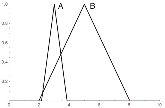
Figure 1. Fuzzy numbers modeling the vague quantity “about 3” (A), and the vague quantity “about 5” (B).

There are different approaches attempting to avoid the problem of the missing totality, mostly they consist of determining a certain ranking index (a crisp number representing the fuzzy number). On the other hand, this leads to a reduction of information. One of the exceptions that we found very elegant and formally founded was defined by Bodenhofer in [46,47]. It works with extending the original fuzzy numbers by constructing their extensional hulls up to the situation when the extended fuzzy numbers can be already ordered regarding their $\alpha$-cuts. Naturally, this approach is very closely connected to the arithmetic of extensional fuzzy numbers and thus, it served for us a motivation, yet our approach comes from a bit more abstract setting and then lands to a particular type of Bodenhofer’s ordering.

3.2. Definitions and Examples

With the goal to encode the necessary vagueness and preserve it as an essential property over the whole computational process, we extend the standard binary ordering relation (between crisp numbers) to a ternary relation ≤ operating on the Cartesian product ${\mathcal{F}}_{\mathcal{S}}\left(\mathbb{R}\right)\times {\mathcal{F}}_{\mathcal{S}}\left(\mathbb{R}\right)\times \mathcal{S}$. As there is never a danger of confusion between the order operating on real numbers and the newly defined order operating on extensional fuzzy sets, the difference will be always clear from the context, we will use the same symbol ≤.

Definition 6.

Let $({\mathcal{F}}_{\mathcal{S}}\left(\mathbb{R}\right),+,-,·{,}^{-1})$ be an MI-prefield of extensional fuzzy numbers with respect to a system $\mathcal{S}$ of nested ⊗-similarities on $\mathbb{R}$. A ternary relation ≤ on ${\mathcal{F}}_{\mathcal{S}}\left(\mathbb{R}\right)\times {\mathcal{F}}_{\mathcal{S}}\left(\mathbb{R}\right)\times \mathcal{S}$ is called an$\mathcal{S}$-ordering on ${\mathcal{F}}_{\mathcal{S}}\left(\mathbb{R}\right)$ provided that

(O1)

$\exists P\in \mathcal{S}:(a_S,a_T,P)\in \le$, (reflexivity)

(O2)

$(a_S,b_T,Q)\in \le \&(b_T,a_S,R)\in \le \Rightarrow a_S-b_T\in I_{\mathcal{S}}^0,(anti-symmetry)$

(O3)

$(a_S,b_T,Q)\in \le \&(b_T,c_U,R)\in \le \Rightarrow \exists P\in \mathcal{S}:(a_S,c_U,P)\in \le ,\left(transitivity\right)$

holds for any $a,b,c\in \mathbb{R}$ and for any $Q,R,S,T,U\in \mathcal{S}$.

Notation 1.

For the case of brevity and clarity, let us introduce the following notation ${(a_S\le b_T)}_U$ denoting the fact that $(a_S,b_T,U)\in \le$. Furthermore, let $a_S\le b_T$ denotes the fact that there exists some $U\in \mathcal{S}$ such that ${(a_S\le b_T)}_U$. This second notation losses the information on which particular $U\in \mathcal{S}$ must be used to obtain a triplet $(a_S,b_T,U)\in \le$ however, in certain situations, such a Boolean information about the order of two fuzzy numbers will be sufficient.

Using Notation 1, the axioms of the $\mathcal{S}$-ordering on ${\mathcal{F}}_{\mathcal{S}}\left(\mathbb{R}\right)$ can be rewritten to a very convenient form:

(O1)

$\exists P\in \mathcal{S}:{(a_S\le a_T)}_P$, (reflexivity)

(O2)

${(a_S\le b_T)}_Q\&{(b_T\le a_S)}_R\Rightarrow a_S-b_T\in I_{\mathcal{S}}^0,(anti-symmetry)$

(O3)

${(a_S\le b_T)}_Q\&{(b_T\le c_U)}_R\Rightarrow \exists P\in \mathcal{S}:{(a_S\le c_U)}_P\left(transitivity\right)$.

Let us recall some examples that first appeared in a bit different formalism in [23,48].

Example 4.

Let $({\mathcal{F}}_{\mathcal{S}}\left(\mathbb{R}\right),+,-,·{,}^{-1})$ be an MI-prefield. Then ${\le }_{max}$ defined as

$${\le }_{max}=\{(a_S,b_T,max(S,T))\mid a,b\in \mathbb{R}\&S,T\in \mathcal{S}\}$$

is an $\mathcal{S}$-ordering on ${\mathcal{F}}_{\mathcal{S}}\left(\mathbb{R}\right)$.

The simple denotation of the fact $(a_S,b_T,max(S,T))\in {\le }_{max}$ is according to Notation 1 very convenient, in particular, we may write ${\left(a_S{\le }_{max}{b}_T\right)}_{max(S,T)}$ or in general $a_S{\le }_{max}{b}_T$.

Relation ${\le }_{max}$ demonstrates an $\mathcal{S}$-ordering reflecting the arithmetic operations: the width of the result of the arithmetic operations determines also the “width of the fuzzy truth” of the proposition stating that $a_S$ is smaller or equal to $b_T$ that is encoded in the third component of the triplet $(a_S,b_T,max(S,T))$. If we mirror this idea into particular arithmetics from Example 3, we get the following ternary relation:

$${\le }_{max}=\{(a_{S_p},b_{S_{p^{\prime }}},min(p,p^{\prime }))\mid a,b\in \mathbb{R}\&S_p,S_{p^{\prime }}\in \mathcal{S}\}$$

where $\mathcal{S}=\{S_p\mid p\in [\ell ,r]\mid \}$ and $S_p$ is given by (1). The demonstration of such an ordering is visualized in Figure 2.

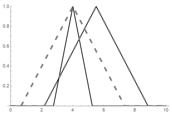
Figure 2. Fuzzy numbers $x_{S_{p^{\prime }}}$ and $y_{S_{p^{″}}}$ determined by the ukasiewicz similarities from Example 3 based on values $x=4$ and $p^{\prime }=0.8$ (“left” solid fuzzy set), $y=5.5$ and $p^{″}=0.3$ (“right” solid fuzzy set). Fuzzy sets $x_{S_{p^{\prime }}}$ and $y_{S_{p^{″}}}$ cannot be ordered by ${\le }_i$ of $\alpha$-cuts however, if we use ${\le }_{max}$, we obtain the dashed fuzzy sets ${\mathrm{EXT}}_{S_{p^{″}}}\left(x_{S_{p^{\prime }}}\right)$ and ${\mathrm{EXT}}_{S_{p^{″}}}\left(y_{S_{p^{″}}}\right)$, respectively, and thus $x_{S_{p^{\prime }}}{\le }_{max}{y}_{S_{p^{″}}}$.

Let us present another example of an $\mathcal{S}$-ordering. It assumes that set of similarities $\mathcal{S}$ has the greatest element.

Example 5.

Let ${\top }_{\mathcal{S}}$ be the greatest element of $\mathcal{S}$, i.e., $R\subseteq {\top }_{\mathcal{S}}$ for all $R\in \mathcal{S}$. Then the ternary relation ${\le }_{{\top }_{\mathcal{S}}}$ given by:

$${\le }_{{\top }_{\mathcal{S}}}=\{(a_S,b_T,{\top }_{\mathcal{S}})\mid a_S,b_T\in {\mathcal{F}}_{\mathcal{S}}\left(\mathbb{R}\right)\&\exists R\in \mathcal{S}:{\mathrm{EXT}}_R\left(a_S\right){\le }_i{\mathrm{EXT}}_R\left(b_T\right)\}$$

is an $\mathcal{S}$-ordering.

The order ${\le }_{{\top }_{\mathcal{S}}}$ orders two fuzzy numbers if there exists a similarity such that the extensional hulls of both fuzzy numbers with respect to this similarity are $\alpha$-cut ordered. Here we see a direct link to the works of Bodenhofer [46,47] that will not be here commented more detail but will turn to be very important in the subsequent sections.

Remark 4.

Note that the particular similarity relation R that was used to order the extensional hulls of two fuzzy numbers via their α-cuts is not mirrored in the information ${\left(a_S{\le }_{{\top }_{\mathcal{S}}}{b}_T\right)}_{{\top }_{\mathcal{S}}}$. This feature, which is not present here, will also turn to be important in the subsequent sections. It actually tells us that ${\le }_{{\top }_{\mathcal{S}}}$ is not that appropriate $\mathcal{S}$-ordering as it does not provide meaningful all three components of the triplet. But it is important to mention that even such structures meet the axiomatic definition of the $\mathcal{S}$-ordering.

Let us consider, e.g., the product t-norm and

$$\mathcal{S}=\{S_p\mid p\in [1,5] \mathrm{and} S_p(x,y)=e^{-p|x-y|}\}.$$

The ordering ${\le }_{{\top }_{\mathcal{S}}}$ can be visually demonstrated by Figure 3 where one can see two extensional fuzzy numbers $4_{S_{2.5}}$ and $5.5_{S_{1.2}}$ (displayed by solid lines) and their extensional hulls ${\mathrm{EXT}}_{S_5}\left(4_{S_2.5}\right)=4_{S_5}$ (left dashed fuzzy set) and ${\mathrm{EXT}}_{S_5}(5.5_{S_{1.2}})=5.5_{S_5}$ (right dashed fuzzy set) that due to their interval-ordering $4_{S_5}{\le }_{i}5.5_{S_5}$ allow the ordering of the original fuzzy numbers ${(4_{S_{2.5}}{\le }_{{\top }_{\mathcal{S}}}5.5_{S_{1.2}})}_{{\top }_{\mathcal{S}}}$.

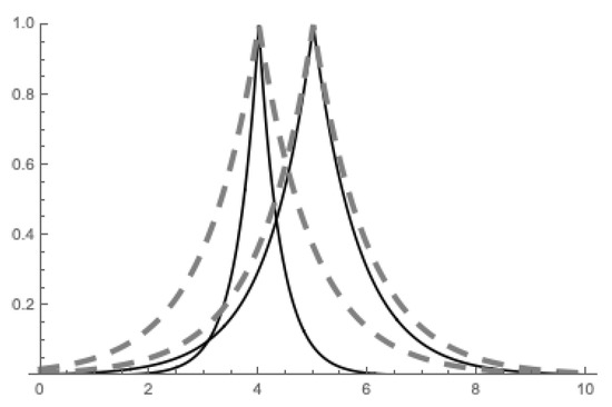
Figure 3. Demonstration of the $\mathcal{S}$-ordering ${\le }_{{\top }_{\mathcal{S}}}$.

Let us equip the system of similarities $\mathcal{S}$ with its bottom element ${\perp }_{\mathcal{S}}$. Then, as $\mathcal{S}$ is the system of nested similarities, it has all infima, i.e., $inf\{S\in \mathcal{C}\mid \mathcal{C}\subseteq \mathcal{S}\}$ exists for any subset $\mathcal{C}$. Then, we can define the ordering that determines the third component of the triplet (the tolerance added to the ordering) as the “narrowest” similarity relation that is sufficient to get ordered $\alpha$-cut of extensional hulls (with respect to this similarity) of the given fuzzy numbers. Mathematically, such a $\mathcal{S}$-ordering ${\le }_{inf}$ will be given by the intersection of all such similarities that lead to the interval-ordering of $\alpha$-cuts of the extensional hulls:

$${\le }_{\cap }=\{(a_S,b_T,E)\mid a_S,b_T\in {\mathcal{F}}_{\mathcal{S}}\left(\mathbb{R}\right)\&E=\cap \{R\in \mathcal{S}\mid {\mathrm{EXT}}_R\left(a_S\right){\le }_i{\mathrm{EXT}}_R\left(b_T\right)\}\}.$$

The visualization of the ordering ${\le }_{\cap }$ is provided in Figure 4.

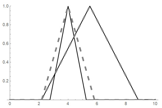
Figure 4. Example of ${\le }_{\cap }$ applied to fuzzy sets from Figure 2.

Let us now come back to the properties of the $\mathcal{S}-orderings$ that were foreshadowed above. In particular, we will recall the so-called pre-order compatibility [23,24] and the real-order compatibility [24].

Definition 7.

Let ≤ be an $\mathcal{S}$-ordering on an MI-prefield $({\mathcal{F}}_{\mathcal{S}}\left(\mathbb{R}\right),+,-,·{,}^{-1})$. Then ≤ is called pre-order compatible if for any $a_S,b_T\in {\mathcal{F}}_{\mathcal{S}}\left(\mathbb{R}\right)$ and $R\in \mathcal{S}$,

$${(a_S\le b_T)}_R\Rightarrow {\mathrm{EXT}}_R\left(a_S\right){\le }_i{\mathrm{EXT}}_R\left(b_T\right).$$

(7)

The name of the pre-order compatibility comes from the close connection to the works of Bodenhofer where the author dealt with pre-orderings of fuzzy sets, see [46,47]. The nature of the property is indeed such that it puts the given $\mathcal{S}$-ordering into the perspective of the above-mentioned pre-orderings. In other words, an $\mathcal{S}$-ordering that is pre-order compatible reflects in the third component of the triplet the width (similarity) of the extension that is necessary to obtain $\alpha$-cut ordered extensional hulls of given fuzzy numbers.

The provided examples of $\mathcal{S}$-orderings ${\le }_{max},{\le }_{{\top }_{\mathcal{S}}},$ and ${\le }_{\cap }$ are examples of pre-order compatible orderings. Now, we will show how easy it is to construct $\mathcal{S}$-orderings that will meet the axioms of Definition 6 but will not be pre-order compatible. There will be two such examples, each of them harming the pre-order compatibility from a different perspective. The first example harms the reflection of the necessary extension.

Example 6.

Let $\mathcal{S}$ be equipped with the bottom element ${\perp }_{\mathcal{S}}$. Then the ternary relation ${\le }_{{\perp }_{\mathcal{S}}}$ given by

$${\le }_{{\perp }_{\mathcal{S}}}=\{(a_S,b_T,{\perp }_{\mathcal{S}})\mid a_S,b_T\in {\mathcal{F}}_{\mathcal{S}}\left(\mathbb{R}\right)\&a\le b\}$$

is an $\mathcal{S}$-ordering that is not pre-order compatible.

The construction of ${\le }_{{\perp }_{\mathcal{S}}}$ focuses only on the core elements—crisp numbers $a,b\in \mathbb{R}$ and ignores the widths of the extensional fuzzy numbers $a_S,b_T\in {\mathcal{F}}_{\mathcal{S}}\left(\mathbb{R}\right)$ constructed above them. In other words, the fuzzy truth (similarity, tolerance) of the proposition $a_S$ is smaller or equal to $b_T$ is thus meaningless, it does not store any information and we get only binary information on the mutual position of a and b.

The other way how the pre-order compatibility can be easily harmed is presented in the following example that reverses the linear order on $\mathbb{R}$.

Example 7.

The ternary relation ${\le }_{max}^{rev}$ defined as follows

$${\le }_{max}^{rev}=\{(a_S,b_T,max(S,T))\mid a_S,b_T\in {\mathcal{F}}_{\mathcal{S}}\left(\mathbb{R}\right)\&b\le a\}$$

is an $\mathcal{S}$-ordering that is not pre-order compatible.

Unlike the $\mathcal{S}$-ordering ${\le }_{{\perp }_{\mathcal{S}}}$, the construction of ${\le }_{max}^{rev}$ reflects the necessary extension and the third component of the triplet would not be meaningful; however, it reverses the order. Thus, we get the information that “about 4” below “about 2”. Please note that reversed order is still order so, nothing wrong in a sense that ${\le }_{max}^{rev}$ would harm Definition 6.

Let us present a lemma which demonstrates the practical impact of the pre-order compatibility as the crucial property of $\mathcal{S}$-orderings.

Lemma 3.

Let ≤ be a pre-order compatible $\mathcal{S}$-ordering on an MI-prefield $({\mathcal{F}}_{\mathcal{S}}\left(\mathbb{R}\right),+,-,·{,}^{-1})$. If $a_S\le b_T$ for certain $S,T\in \mathcal{S}$ then $a\le b$.

Proof. 

Let ≤ be pre-order compatible. Then $a_S\le b_T$ (according to Notation 1) means that there exists $U\in \mathcal{S}$ such that ${\mathrm{EXT}}_R\left(a_S\right){\le }_i{\mathrm{EXT}}_R\left(b_T\right)$. Let us expand the formula for the extensional hull of $a_S$

$$\begin{array}{c}{\mathrm{EXT}}_R\left(a_S\right)\left(z\right)=\underset{y\in \mathbb{R}}{\bigvee }{a}_S\left(y\right)\otimes R(y,z)\end{array}$$

and let us determine its core, i.e., let us put it equal to 1:

$$\begin{array}{c}1=\underset{y\in \mathbb{R}}{\bigvee }{a}_S\left(y\right)\otimes R(y,z)=\underset{y\in \mathbb{R}}{\bigvee }S(a,y)\otimes R(y,z)\le \\ \underset{y\in \mathbb{R}}{\bigvee }max(S,R)(a,y)\otimes max(S,R)(y,z)\le max(S,R)(a,z),\end{array}$$

Due to the separability property assumed in Convention 1, we get $max(S,R)(a,z)=1$ if and only if $a=z$. Thus, the sought core ($\alpha$-cut for $\alpha =1$) is ${\mathrm{EXT}}_R{\left(a_S\right)}_1=\left\{a\right\}$. Analogously, we get ${\mathrm{EXT}}_R{\left(b_T\right)}_1=\left\{b\right\}$. Finally, ${\mathrm{EXT}}_R{\left(a_S\right)}_1\le {\mathrm{EXT}}_R{\left(b_T\right)}_1$ can be directly rewritten as $a\le b$, which concludes the proof. □

Example 8.

Let us demonstrate Lemma 3 on examples. Consider the case depicted in Figure 2. For the pre-order compatible $\mathcal{S}$-ordering ${\le }_{max}$, the assumptions of the lemma are met, and it can be seen that $x_{S_{p^{\prime }}}{\le }_{max}{y}_{S_{p^{″}}}$ as well as $x\le y$ holds. For the $\mathcal{S}$-ordering ${\le }_{max}^{rev}$ the assumption on the pre-order compatibility is dropped and from $y_{S_{p^{″}}}{\le }_{max}^{rev}{x}_{S_{p^{\prime }}}$ we cannot deduce that $y\le x$ as the opposite is true.

However, Lemma 3 claims only one direction implication, not the equivalence, and so, it does not exclude the possibility of a pre-order $\mathcal{S}$-ordering that would preserve the implication. Indeed, consider ${\le }_{{\perp }_{\mathcal{S}}}$ that is defined in such a way that from $x_{S_{p^{\prime }}}{\le }_{{\perp }_{\mathcal{S}}}{y}_{S_{p^{″}}}$ we can easily deduce $x\le y$.

Naturally, one may revisit the pre-order compatibility defining Formula (7) and consider it with the equivalence instead of the implication. However, such a condition would be too restrictive and the only order that would in general meet such a requirement would be ${\le }_{\cap }$. However, we can weaken the opposite implication and require only weaken version that ensures some dependence on the order of the real line but without reflecting the particular similarity. The reflection of the necessarily used similarity mirrored only in one of the implications—the one in Formula (7)—will turn to be sufficient, see Section 4.

Definition 8.

Let ≤ be an $\mathcal{S}$-ordering on an MI-prefield $({\mathcal{F}}_{\mathcal{S}}\left(\mathbb{R}\right),+,-,·{,}^{-1})$. Then ≤ is called real-order compatible if for any $a_S,b_T\in {\mathcal{F}}_{\mathcal{S}}\left(\mathbb{R}\right)$ and $R\in \mathcal{S}$ the following holds

$${\mathrm{EXT}}_R\left(a_S\right){\le }_i{\mathrm{EXT}}_R\left(b_T\right)\Rightarrow a_S\le b_T.$$

(8)

The $\mathcal{S}$-orderings ${\le }_{max},{\le }_{{\top }_{\mathcal{S}}}$, ${\le }_{\cap }$, and ${\le }_{{\perp }_{\mathcal{S}}}$ presented above are real-order compatible however, for example, ${\le }_{max}^{rev}$ is not real-order compatible. Can we construct an $\mathcal{S}$-ordering that is unlike ${\le }_{max}^{rev}$ pre-order compatible however, it is not real-order compatible? Indeed, the following example focusing only on the left points of the supports provides such an example.

Example 9.

The ternary relation ${\le }_{max}^L$ defined as follows

$${\le }_{max}^L=\{(a_S,b_T,max(S,T))\mid a_S,b_T\in {\mathcal{F}}_{\mathcal{S}}\left(\mathbb{R}\right)\&inf\mathrm{Supp}\left(a_S\right)\le inf\mathrm{Supp}\left(b_T\right)\}$$

is an $\mathcal{S}$-ordering that is pre-order compatible but it is not real-order compatible.

Now, putting both compatibilities together gives us an $\mathcal{S}$-ordering with properties sufficient for proving further results.

Definition 9.

If an $\mathcal{S}$-ordering is pre-order compatible and real-order compatible, it is said to be strongly compatible.

Remark 5.

The $\mathcal{S}$-orderings ${\le }_{max},{\le }_{{\top }_{\mathcal{S}}}$, and ${\le }_{\cap }$ presented above are strongly compatible.

Another crucial property is the linearity or totality of the order. Naturally, also this property deserves to be incorporated into the context of $\mathcal{S}$-orderings.

Definition 10.

Consider an MI-prefield $({\mathcal{F}}_{\mathcal{S}}\left(\mathbb{R}\right),+,-,·{,}^{-1})$ and an $\mathcal{S}$-ordering ≤ on ${\mathcal{F}}_{\mathcal{S}}\left(\mathbb{R}\right)$. Then ≤ is called total if the following holds for arbitrary $a_S,b_T\in {\mathcal{F}}_{\mathcal{S}}\left(\mathbb{R}\right)$:

$$a_S\le b_{T}or{b}_T\le a_S.$$

(totality)

Let us focus on the relationship of the real-order compatibility and the totality.

Proposition 1.

Let $({\mathcal{F}}_{\mathcal{S}}\left(\mathbb{R}\right),+,-,·{,}^{-1})$ be an MI-prefield and let ≤ be an $\mathcal{S}$-ordering on ${\mathcal{F}}_{\mathcal{S}}\left(\mathbb{R}\right)$. If ≤ is real-order compatible then it is also total.

Proof. 

We prove the proposition by contradiction. Let us assume that for some $a_S,b_T\in {\mathcal{F}}_{\mathcal{S}}\left(\mathbb{R}\right)$ it holds that $a_S\nleqq b_T\&b_T\nleqq a_S$.

The assumption $a_S\nleqq b_T$ means that there does not exist any $R\in \mathcal{S}$ such that ${\mathrm{EXT}}_R\left(a_S\right){\le }_i{\mathrm{EXT}}_R\left(b_T\right)$. Indeed, if it existed, the real-order compatibility would lead to the contradiction with the assumption. As for any $\alpha$, the $\alpha$-cuts ${\mathrm{EXT}}_R{\left(a_S\right)}_{\alpha }$ and ${\mathrm{EXT}}_R{\left(b_T\right)}_{\alpha }$ are of the same width and ${\mathrm{EXT}}_R\left(a_S\right){\nleqq }_i{\mathrm{EXT}}_R\left(b_T\right)$ holds then necessarily ${\mathrm{EXT}}_R\left(b_T\right){\le }_i{\mathrm{EXT}}_R\left(a_S\right)$ which, due to the real-order compatibility, means that $b_T\le a_S$. □

4. Properties of $\mathcal{S}$-Orderings

4.1. Wang–Kerre Properties of Orderings of Fuzzy Numbers

As the orderings and rankings of fuzzy numbers attracted significant interest of the researcher, it is not surprising that some of them aimed at their properties. Many ordering techniques rely on comparing certain crisp numbers (indices or representative numbers) instead of comparing the original fuzzy numbers [49]. The natural consequence is a partiality of such orderings that is viewed as a problem by some authors. This is sometimes heuristically overcome by using multiple indices. This article does not focus on an exhaustive survey of all such methods and we are convinced that every single approach has its motivation justifying its existence. However, if we intend to apply the proposed arithmetic of extensional fuzzy numbers to the problem of fuzzy interpolation where orderings of fuzzy numbers play a crucial role, we need to know more about it. In particular, we should investigate under which conditions our approach preserves the most natural properties.

We have adopted the investigations of Wang and Kerre [49,50] as the starting point. This step is rather natural as the authors set up the most intuitive properties of orderings of fuzzy numbers and our goal is not to mimic such works but to investigate our technique in such a generally accepted framework.

Remark 6.

No matter if using indices or not, several techniques for ordering/ranking of fuzzy numbers operate on a finite subset of (reference) fuzzy numbers to which the ordering can be applied. Therefore, the ordering of two fuzzy numbers compares both to the reference set first. This fact is mirrored in the Wang–Kerre properties (axioms) recalled below. When mimicking the properties in our formalism of extensional fuzzy numbers, the properties will need to be slightly modified to drop the reference set(s), one of the properties will become totally redundant without considering the reference set.

Wang–Kerre properties: Let us consider $\mathcal{F}\left(\mathbb{R}\right)$ and let $H,H_1,$ and $H_2$ be arbitrary finite subsets of $\mathcal{F}\left(\mathbb{R}\right)$ (the reference sets). Furthermore, let $h\in \mathbb{R}$. Then

A1:

$A⪯A$, for $A\in H$;

A2:

$A⪯BandB⪯A\Rightarrow A\sim B$, for $A,B\in H$;

A3:

$A⪯BandB⪯C\Rightarrow A⪯C$, for $A,B,C\in H$;

A4:

$sup\mathrm{Supp}\left(A\right)\le inf\mathrm{Supp}\left(B\right)\Rightarrow A⪯B$, for $A,B\in H$;

A5:

Let $A,B\in H_1\cap H_2$. Then $A⪯Bin{H}_1\iff A⪯Bin{H}_2$;

A6:

Let $A⪯Bin{H}_1=\{A,B\}$. Then $A+C⪯B+Cin{H}_2=\{A+C,B+C\}$;

A7:

Let $0\le h$ and $A,B,h·A,h·B\in H$.

Then $A⪯Bin{H}_1=\{A,B\}impliesh·A⪯h·Bin{H}_2=\{h·A,h·B\}$.

For the sake of brevity, when recalling the Wang–Kerre properties A1–A7, we dared to relax the precise definitions of the used symbols ⪯ and ∼ as the main motivation is to provide the readers with the ideas that must be accommodated to a different formalism in the framework of extensional fuzzy numbers anyhow.

4.2. Wang–Kerre Properties for $\mathcal{S}$-Orderings and Their Preservation

The implementation of the above-recalled Wang–Kerre properties to the framework of $\mathcal{S}$-orderings and extensional fuzzy numbers requires some modifications, for example, any use of reference sets is meaningless, $\mathcal{S}$-orderings of not use them to order objects from ${\mathcal{F}}_{\mathcal{S}}\left(\mathbb{R}\right)$ at all. Consequently, axiom A5 is omitted from our consideration as whenever no reference set is used, it is always automatically fulfilled. Otherwise, one can see that the modification is only formal and preserving the same ideas and motivations.

Let $a_S,b_T,c_R\in {\mathcal{F}}_{\mathcal{S}}\left(\mathbb{R}\right)$ and let $h\in \mathbb{R}$. Then the modified Wang–Kerre properties are given as follows:

A1’:

$a_S\le a_S$;

A2’:

$a_S\le b_T\mathrm{and}{b}_T\le a_S\Rightarrow (a_S-b_T)\in I_{\mathcal{S}}^0$;

A3’:

$a_S\le b_T\mathrm{and}{b}_T\le c_R\Rightarrow a_S\le c_R$;

A4’:

$sup\mathrm{Supp}\left(a_S\right)\le inf\mathrm{Supp}\left(b_T\right)\Rightarrow a_S\le b_T$;

A6’:

$a_S\le b_T\Rightarrow a_S+c_R\le b_T+c_R$;

A7’:

$0\le h$ and $a_S\le b_T\Rightarrow h·a_S\le h·b_T$;

The goal of the subsequent parts of the article is to investigate under which conditions an $\mathcal{S}$-ordering preserves the properties A1’–A7’.

Proposition 2.

Let ≤ be an $\mathcal{S}$-ordering. Then it preserves properties A1’, A2’, and A3’.

Proof. 

Using the reflexivity axiom (O1) from Definition 6, for any $S,T\in \mathcal{S}$ there must exist $P\in \mathcal{S}$ such that ${(a_S\le a_T)}_P$ which implies $a_S\le a_T$. It suffices to put $S=T$ to complete the proof of A1’.

The anti-symmetry axiom (O2) from Definition 6 states that ${(a_S\le b_T)}_Q$ and ${(b_T\le a_T)}_R$ implies $a_S-b_T\in I_{\mathcal{S}}^0$. As it holds for any for any $S,T,Q,R\in \mathcal{S}$, we directly obtain the proof of A2’.

Finally, the transitivity axiom (O3) from Definition 6 states that ${(a_S\le b_T)}_Q$ and ${(b_T\le c_U)}_R$ implies ${(a_S\le c_U)}_P$ for some $P\in \mathcal{S}$. As it holds for any for any $S,T,U,Q,R\in \mathcal{S}$, we directly obtain the proof of A3’. □

The preservation of A4’ is not as automatic as the preservation of A1’-A3’ that stemmed directly from the axioms (O1)-(O3). An additional property must be assumed.

Proposition 3.

Let ≤ be a real-order compatible $\mathcal{S}$-ordering. Then it preserves the property A4’.

Proof. 

If $sup\mathrm{Supp}\left(a_S\right)\le inf\mathrm{Supp}\left(b_T\right)$ holds, we immediately get the interval-ordering for all $\alpha$-cuts of both fuzzy numbers: $a_S{\le }_i{b}_T$ or equivalently ${\mathrm{EXT}}_S\left(a\right){\le }_i{\mathrm{EXT}}_T\left(b\right)$ by Lemma 1. Put $R=min(S,T)$. Recall that the composition of similarities U and V is defined as $U\circ V(x,y)={\bigvee }_{z\in \mathbb{R}}U(x,z)\otimes V(z,y)$. Obviously, we have $S=S\circ R$ and $T=T\circ R$, where $R=min(S,T)$. Indeed, assume that $R=S$. Then $S=S\circ S$ follows immediately from the transitivity of S. In addition, we have

$$\begin{array}{c}T\circ S(x,y)=\underset{z\in \mathbb{R}}{\bigvee }T(x,z)\otimes S(z,y)\ge T(x,y)\otimes S(y,y)=T(x,y)\otimes 1=T(x,y),x,y\in \mathbb{R},\end{array}$$

therefore, $T\subseteq T\circ S$. On the other side, from $S\subseteq T$ and the transitivity of T, we have

$$\begin{array}{c}T\circ S(x,y)=\underset{z\in \mathbb{R}}{\bigvee }T(x,z)\otimes S(z,y)\le \underset{z\in \mathbb{R}}{\bigvee }T(x,z)\otimes T(z,y)=T(x,y),x,y\in \mathbb{R},\end{array}$$

therefore, $T\circ S\subseteq T$, and hence, we obtain $T=T\circ S$. Similarly, one can show the equalities for $R=T$. Since ${\mathrm{EXT}}_S\left(a\right){\le }_i{\mathrm{EXT}}_T\left(b\right)$, using the previous equalities, we simply find that ${\mathrm{EXT}}_R\left(a_S\right)={\mathrm{EXT}}_{S\circ R}\left(a\right)={\mathrm{EXT}}_S\left(a\right){\le }_i{\mathrm{EXT}}_T\left(b\right)={\mathrm{EXT}}_{T\circ R}\left(b\right)={\mathrm{EXT}}_R\left(b_T\right)$ which jointly with the real-order compatibility leads to $a_S\le b_T$. □

Example 10.

Let us again demonstrate Proposition 3 on examples. Let us consider two (disjoint) extensional fuzzy numbers such that $sup\mathrm{Supp}\left(a_S\right)\le inf\mathrm{Supp}\left(b_T\right)$. For the real-order compatible $\mathcal{S}$-ordering ${\le }_{max}$, we easily obtain $a_S{\le }_{max}{b}_T$. However, for the $\mathcal{S}$-ordering ${\le }_{max}^{rev}$ that is not real-order compatible, we get the opposite, in particular $b_T{\le }_{max}^{rev}{a}_S$.

The real-order compatibility turned to be useful in proving the preservation of A4’ however, it is not sufficient to prove the preservation of A5’. As it will be shown, we will need to use “the other direction” encoded in the pre-order compatibility and thus, the strong compatibility will be assumed.

Proposition 4.

Let ≤ be a strongly compatible $\mathcal{S}$-ordering, and let any similarity from $\mathcal{S}$ be shift-invariant. Then it preserves the property A6’.

Proof. 

Let $a_S,b_T,c_R\in {\mathcal{F}}_{\mathcal{S}}\left(\mathbb{R}\right)$ and let $a_S\le b_T$ where ≤ is strongly compatible. Put $U=max(S,T,R)$. From the reflexivity axiom (O1) we have ${(a_U\le a_S)}_P$ and ${(b_T\le b_U)}_Q$ for certain similarities $P,Q\in \mathcal{S}$, i.e., $a_U\le a_S$ and $b_T\le b_U$, and by the transitivity axiom (O3), we find that ${(a_U\le b_U)}_V$ for a certain similarity $V\in \mathcal{S}$, i.e., $a_U\le b_U$. In what follows, for simplicity, we do not mention the existence of similarities P and Q in $\mathcal{S}$, and we will directly write $\mathcal{S}$-ordering. Since ≤ is strong compatible, there exists $W\in \mathcal{S}$ such that ${\mathrm{EXT}}_W\left(a_U\right){\le }_i{\mathrm{EXT}}_W\left(b_U\right)$. We show that ${\mathrm{EXT}}_W\left({(a+c)}_U\right){\le }_i{\mathrm{EXT}}_W\left({(b+c)}_U\right)$ also holds. By Lemma 2, one can simply check that for any $x\in \mathbb{R}$, there exists $x^{\prime }\in \mathbb{R}$ such that $x\le x^{\prime }$ and

$${\mathrm{EXT}}_W\left(a_U\right)(x-c)={\bigvee }_{y\in \mathbb{R}}U(a,y)\otimes W(y,x-c)\le {\bigvee }_{z\in \mathbb{R}}U(b,z)\otimes W(z,x^{\prime }-c)={\mathrm{EXT}}_W\left(b_U\right)(x^{\prime }-c)$$

(9)

and vice versa, for any $x^{\prime }\in \mathbb{R}$, there exists $x\in \mathbb{R}$ such that $x\le x^{\prime }$ and

$${\mathrm{EXT}}_W\left(b_U\right)(x^{\prime }-c)={\bigvee }_{z\in \mathbb{R}}U(b,z)\otimes W(z,x^{\prime }-c)\le {\bigvee }_{y\in \mathbb{R}}U(a,y)\otimes W(y,x-c)={\mathrm{EXT}}_W\left(a_U\right)(x-c).$$

(10)

Hence, and using the shift-invariance of U and W, e.g., $U(a+c,y)=U(a,y-c)$ or $W(y,x)=W(y-c,x-c)$, if $x\in \mathbb{R}$, then there exists $x^{\prime }\in \mathbb{R}$ such that $x\le x^{\prime }$ and (9) holds, which implies

$$\begin{array}{cc}\hfill {\mathrm{EXT}}_W\left({(a+c)}_U\right)\left(x\right)& =\underset{y\in \mathbb{R}}{\bigvee }U(a+c,y)\otimes W(y,x)=\underset{y\in \mathbb{R}}{\bigvee }U(a,y-c)\otimes W(y-c,x-c)\hfill \\ \hfill & ={\mathrm{EXT}}_W\left(a_U\right)(x-c)\le {\mathrm{EXT}}_W\left(b_U\right)(x^{\prime }-c)=\underset{z\in \mathbb{R}}{\bigvee }U(b,z-c)\otimes W(z-c,x^{\prime }-c)\hfill \\ \hfill & =\underset{z\in \mathbb{R}}{\bigvee }U(b+c,z)\otimes W(z,x^{\prime })={\mathrm{EXT}}_W\left({(b+c)}_U\right)\left(x^{\prime }\right).\hfill \end{array}$$

Similarly, if $x^{\prime }\in \mathbb{R}$, then there exists $x\in \mathbb{R}$ such that $x\le x^{\prime }$ and (10) holds, which implies

$$\begin{array}{cc}\hfill {\mathrm{EXT}}_W\left({(b+c)}_U\right)\left(x^{\prime }\right)& =\underset{z\in \mathbb{R}}{\bigvee }U(b+c,z)\otimes W(z,x^{\prime })=\underset{z\in \mathbb{R}}{\bigvee }U(b,z-c)\otimes W(z-c,x^{\prime }-c)\hfill \\ \hfill & ={\mathrm{EXT}}_W\left(b_U\right)(x^{\prime }-c)\le {\mathrm{EXT}}_W\left(a_U\right)(x-c)=\underset{y\in \mathbb{R}}{\bigvee }U(b,y-c)\otimes W(y-c,x-c)\hfill \\ \hfill & =\underset{y\in \mathbb{R}}{\bigvee }U(b+c,y)\otimes W(y,x)={\mathrm{EXT}}_W\left({(b+c)}_U\right)\left(x\right).\hfill \end{array}$$

By Lemma 2, we find that ${\mathrm{EXT}}_W\left({(a+c)}_U\right){\le }_i{\mathrm{EXT}}_W\left({(b+c)}_U\right)$, and using the real-order compatibility, we obtain ${(a+c)}_U\le {(b+c)}_U$. Using reflexivity (O1), it holds that ${(a+c)}_{max(S,R)}\le {(a+c)}_U$ and ${(b+c)}_U\le {(b+c)}_{max(T,R)}$, and by transitivity (O3), we obtain $a_S+c_R={(a+c)}_{max(S,R)}\le {(b+c)}_{max(T,R)}=b_T+c_R$. □

Example 11.

Let us demonstrate Proposition 4 on some examples. Let us again consider the case depicted in Figure 2 with $x_{S_{p^{\prime }}}$ and $y_{S_{p^{″}}}$ that are shift-invariant. Furthermore, let us consider $z_{S_{p^{″\prime }}}$ such that z is an arbitrary number from $\mathbb{R}$ and $S_{p^{″\prime }}\ge max(S_{p^{\prime }},S_{p^{″}})$ (i.e., $p^{″\prime }<min(p^{\prime },p^{″})$ ).

If we consider a strongly compatible $\mathcal{S}$-ordering ${\le }_{max}$ then we have $x_{S_{p^{\prime }}}{\le }_{max}{y}_{S_{p^{″}}}$ and easily, we can check that also ${(x+z)}_{S_{p^{‴}}}{\le }_{max}{(y+z)}_{S_{p^{‴}}}$ holds, where the left-hand side is equal to $x_{S_{p^{\prime }}}+z_{S_{p^{‴}}}$ and the right-hand side is equal to $y_{S_{p^{″}}}+z_{S_{p^{‴}}}$.

Now, let us consider the $\mathcal{S}$-ordering ${\le }_{max}^L$ and that is not strongly compatible, see Example 9. Due to the position of the left-hand sides of the supports, the following $y_{S_{p^{″}}}{\le }_{max}^L{x}_{S_{p^{\prime }}}$ holds. However, $x_{S_{p^{\prime }}}+z_{S_{p^{‴}}}={(x+z)}_{S_{p^{‴}}}$ and $y_{S_{p^{″}}}+z_{S_{p^{‴}}}={(y+z)}_{S_{p^{‴}}}$ so, we get two extensional fuzzy number of the same width and as $(x+y)\le (y+z)$, also the left-hand sides of the supports are ordered in this way. Consequently, ${(x+z)}_{S_{p^{‴}}}{\le }_{max}^L{(y+z)}_{S_{p^{‴}}}$ which harms the property A6’.

Again, note that the proposition states only one implication but the opposite implication does not hold. Therefore, if we consider the $\mathcal{S}$-ordering that reverses the order ${\le }_{max}^{rev}$, we get $y_{S_{p^{″}}}{\le }_{max}^L{x}_{S_{p^{\prime }}}$ as well as ${(y+z)}_{S_{p^{‴}}}{\le }_{max}^L{(x+z)}_{S_{p^{‴}}}$ and thus, A6’ is preserved even though ${\le }_{max}^{rev}$ is not strongly compatible.

The last axiom that must be checked will be preserved again under the assumption of the strong compatibility. Additionally, the presence of the crisp bottom element in the considered MI-pregroup will be assumed.

Proposition 5.

Let ≤ be a strongly compatible $\mathcal{S}$-ordering on an MI-prefield $({\mathcal{F}}_{S_{\infty }}\left(\mathbb{R}\right),+,-,·{,}^{-1})$ with the crisp bottom element. Then it preserves the property A7’.

Proof. 

As $S_{\infty }$ contains the crisp bottom element ${\perp }_{\mathcal{S}}$ (classical equality), we may incorporate the representation of the scalar multiplication in ${\mathcal{F}}_{S_{\infty }}\left(\mathbb{R}\right)$:

$$h·a_S=h_{{\perp }_{\mathcal{S}}}·a_S={(h·a)}_{max(S,{\perp }_{\mathcal{S}})}={(h·a)}_S.$$

If $a_S\le b_T$ and ≤ is pre-order compatible, then $a\le b$ and necessarily $h·a\le h·b$ for any $h>0$. Since ${\left({\mathrm{EXT}}_{{\perp }_{\mathcal{S}}}\left({(h·a)}_{{\perp }_{\mathcal{S}}}\right)\right)}_{\alpha }=\{h·a\}$ and ${\left({\mathrm{EXT}}_{{\perp }_{\mathcal{S}}}\left({(h·b)}_{{\perp }_{\mathcal{S}}}\right)\right)}_{\alpha }=\{h·b\}$ for any $\alpha \in (0,1]$, we find that ${\mathrm{EXT}}_{{\perp }_{\mathcal{S}}}\left({(h·a)}_{{\perp }_{\mathcal{S}}}\right){\le }_i{\mathrm{EXT}}_{{\perp }_{\mathcal{S}}}{(h·b)}_{{\perp }_{\mathcal{S}}})$, which implies ${(h·a)}_{{\perp }_{\mathcal{S}}}\le {(h·b)}_{{\perp }_{\mathcal{S}}}$ as a consequence of the real-order compatibility. Using the reflexivity axiom (O1), we obtain ${(h·a)}_S\le {(h·a)}_{{\perp }_{\mathcal{S}}}$ and ${(h·b)}_{{\perp }_{\mathcal{S}}}\le {(h·b)}_T$, and from the transitivity axiom (O3), we find that ${(h·a)}_S\le {(h·b)}_T$. □

Corollary 1.

Let ≤ be a strongly compatible $\mathcal{S}$-ordering on an MI-prefield $({\mathcal{F}}_{S_{\infty }}\left(\mathbb{R}\right),+,-,·{,}^{-1})$ with the crisp bottom element. Then it simultaneously preserves axioms A1’-A4’ and A6’-A7.

Proof. 

We have to prove that A6’ remains true if the shift-invariance is omitted in ${\mathcal{F}}_{S_{\infty }}\left(\mathbb{R}\right)$ (cf. Proposition 4). Let $a_S,b_T,c_R\in {\mathcal{F}}_{S_{\infty }}\left(\mathbb{R}\right)$. As with the proof of Proposition 5, if $a_S\le b_T$ and ≤ is pre-order compatible, then $a\le b$ and necessarily $a+c\le b+c$. Since ${\mathrm{EXT}}_{{\perp }_{\mathcal{S}}}\left({(a+c)}_{{\perp }_{\mathcal{S}}}\right){\le }_i{\mathrm{EXT}}_{{\perp }_{\mathcal{S}}}{(b+c)}_{{\perp }_{\mathcal{S}}})$, we find that ${(a+c)}_{{\perp }_{\mathcal{S}}}\le {(b+c)}_{{\perp }_{\mathcal{S}}}$ because of the real-order compatibility. Using the reflexivity axiom (O1), we obtain $a_S+c_R={(a+c)}_{max(S,R)}\le {(a+c)}_{{\perp }_{\mathcal{S}}}$ and ${(b+c)}_{{\perp }_{\mathcal{S}}}\le {(b+c)}_{max(T,R)}=b_T+c_R$, and from the transitivity axiom (O3), we obtain $a_S+c_R\le b_T+c_R$. □

Corollary 1 directly gathers the results from Propositions 2–5 and shows an elegant and safe way how to construct a system of similarities and an $\mathcal{S}$-ordering that is safe in the sense of meeting all the preferable properties. Indeed, the list of assumptions may seem high, but it is not restrictive at all. As we showed above, the most natural and intuitive $\mathcal{S}$-orderings are strongly compatible and analogously, including the crisp equality as the crisp bottom element to the system of nested similarities is more natural than starting from a wider bottom element.

Definition 11.

Let $({\mathcal{F}}_{\mathcal{S}}\left(\mathbb{R}\right),+,-,·{,}^{-1})$ be an MI-prefield, and let ≤ be an $\mathcal{S}$-ordering on ${\mathcal{F}}_{\mathcal{S}}\left(\mathbb{R}\right)$. The structure $({\mathcal{F}}_{\mathcal{S}}\left(\mathbb{R}\right),+,-,·{,}^{-1},\le )$ will be called an$\mathcal{S}$-ordered MI-prefield provided that for any $a_S,b_T,c_R\in {\mathcal{F}}_{\mathcal{S}}\left(\mathbb{R}\right)$ and $U,V\in \mathcal{S}$, it holds that

(P1) 

$a_S\le b_T\Rightarrow a_S+c_U\le b_T+b_U$,

(P2) 

$0_U\le a_S$ and $0_V\le b_T\Rightarrow \exists W\in \mathcal{S}:0_W\le a_S·b_T$.

The following statement shows that the shift-invariance of similarities and strong compatibility of $\mathcal{S}$-ordering are sufficient conditions to get a $\mathcal{S}$-ordered MI-prefield.

Proposition 6.

Let $({\mathcal{F}}_{\mathcal{S}}\left(\mathbb{R}\right),+,-,·{,}^{-1})$ be an MI-prefield such that any similarity from $\mathcal{S}$ is shift-invariant, and let ≤ be a strongly compatible $\mathcal{S}$-ordering on ${\mathcal{F}}_{\mathcal{S}}\left(\mathbb{R}\right)$. Then $({\mathcal{F}}_{\mathcal{S}}\left(\mathbb{R}\right),+,-,·{,}^{-1},\le )$ is an $\mathcal{S}$-ordered MI-prefield.

Proof. 

(P1) follows from Proposition 4. Let $0_U\le a_S$ and $0_V\le b_T$ for $a_S,b_T\in {\mathcal{F}}_{\mathcal{S}}\left(\mathbb{R}\right)$ and $U,V\in \mathcal{S}$. According to reflexivity of $\mathcal{S}$-ordering, we obtain $0_S\le 0_U$ and $0_T\le 0_V$, and by transitivity, we find that $0_S\le a_S$ and $0_T\le b_T$. Denote $R=max(S,T)$. Then we have $0_R=0_S·0_T$ and ${\left(ab\right)}_R=a_S·b_T$. We will show that $0_R\le {\left(ab\right)}_S$. Since ≤ is strongly compatible, as a consequence of the real-order compatibility, it is sufficient to show that there exists $W\in \mathcal{S}$ such that

$$\begin{array}{c}{\mathrm{EXT}}_W\left(0_R\right){\le }_i{\mathrm{EXT}}_W\left({\left(ab\right)}_R\right).\end{array}$$

(11)

By Lemma 2, we will show that for any $x\in \mathbb{R}$ there exists $x^{\prime }\in \mathbb{R}$ such that $x\le x^{\prime }$ and

$$\begin{array}{c}\underset{y\in \mathbb{R}}{\bigvee }R(0,y)\otimes W(y,x)\le \underset{z\in \mathbb{R}}{\bigvee }R(ab,z)\otimes W(z,x^{\prime })\end{array}$$

(12)

and vice versa, for any $x^{\prime }\in \mathbb{R}$ there exists $x\in \mathbb{R}$ such that $x\le x^{\prime }$ and

$$\begin{array}{c}\underset{z\in \mathbb{R}}{\bigvee }R(ab,z)\otimes W(z,x^{\prime })\le \underset{y\in \mathbb{R}}{\bigvee }R(0,y)\otimes W(y,x).\end{array}$$

(13)

Let $W\in \mathcal{S}$ be an arbitrary similarity. Since R and W are shift-invariant, for any $x\in \mathbb{R}$, we obtain

$$\begin{array}{c}\underset{y\in \mathbb{R}}{\bigvee }R(0,y)\otimes W(y,x)=\underset{y\in \mathbb{R}}{\bigvee }R(ab,y+ab)\otimes W(y+ab,x+ab)=\underset{y\in \mathbb{R}}{\bigvee }R(ab,z)\otimes W(z,x^{\prime }),\end{array}$$

where we put $x^{\prime }=x+ab$. Since R is strongly compatible, by Lemma 3 we find that $0\le a$ and $0\le b$, which implies $x\le x+ab=x^{\prime }$. Similarly, for any $x^{\prime }\in \mathbb{R}$, we obtain

$${\bigvee }_{z\in \mathbb{R}}R(ab,z)\otimes W(z,x^{\prime })={\bigvee }_{z\in \mathbb{R}}R(0,z-ab)\otimes W(z-ab,x^{\prime }-ab)={\bigvee }_{y\in \mathbb{R}}R(0,y)\otimes W(y,x),$$

(14)

where we put $x=x^{\prime }-ab$, and thus $x\le x^{\prime }$. By Lemma 2, we obtain (11) and thus $0_R\le {\left(ab\right)}_R=a_S·b_T$, which concludes the proof of (P2). □

Example 12.

Let $({\mathcal{F}}_{{\mathcal{S}}_{\infty }}\left(\mathbb{R}\right),+,-,·{,}^{-1})$ be the MI-prefield with ${\mathcal{S}}_{\infty }=\{S_p\mid p\in (0,+\infty ]\}$, where $S_p$ is given by (1) for any $0<p<+\infty$ and $S_{\infty }$ is the crisp equality (see, Remark 3), which is enriched by a strong compatible ${\mathcal{S}}_{\infty }$-ordering ≤. Since any similarity from ${\mathcal{S}}_{\infty }$ is shift-invariant (see, Example 1), by the previous proposition, $({\mathcal{F}}_{{\mathcal{S}}_{\infty }}\left(\mathbb{R}\right),+,-,·{,}^{-1},\le )$ is an ordered MI-prefield.

Since $\mathcal{S}$-ordering on an MI-prefield ${\mathcal{F}}_{\mathcal{S}}\left(\mathbb{R}\right)$ is determined by the set $\mathcal{S}$ of similarities that is referred in the index of the MI-prefield, for convenience, we will omit $\mathcal{S}$ in “$\mathcal{S}$-ordered MI-prefield” and write only “ordered MI-prefield”. In the following definition, we introduce the isomorphism of ordered MI-prefields which is used in our demonstration of fuzzy interpolation. As with algebraic literature, for convenience, we do not distinguish the operations and orderings of ordered MI-prefields using indexes if no confusion can appear.

Definition 12.

Let $({\mathcal{F}}_{{\mathcal{S}}_1}\left(\mathbb{R}\right),+,-,·{,}^{-1},\le )$ and $({\mathcal{F}}_{{\mathcal{S}}_2}\left(\mathbb{R}\right),+,-,·{,}^{-1},\le )$ be ordered MI-prefields. A map $h:{\mathcal{F}}_{{\mathcal{S}}_1}\left(\mathbb{R}\right)\to {\mathcal{F}}_{{\mathcal{S}}_2}\left(\mathbb{R}\right)$ is a homomorphism of ordered MI-prefields provided that

(H1) 

$h(a_S+b_T)=h\left(a_S\right)+h\left(b_T\right)$, $h\left(0_{{\perp }_{{\mathcal{S}}_1}}\right)=0_{{\perp }_{{\mathcal{S}}_2}}$ and $h(-a_S)=-h\left(a_S\right)$ for any $a_S,b_T\in {\mathcal{F}}_{{\mathcal{S}}_1}\left(\mathbb{R}\right)$;

(H2) 

$h(a_S·b_T)=h\left(a_S\right)·h\left(b_T\right)$, $h\left(1_{{\perp }_{{\mathcal{S}}_1}}\right)=1_{{\perp }_{{\mathcal{S}}_2}}$ and $h\left({\left(a_S\right)}^{-1}\right)=h^{-1}\left(a_S\right)$ for any $a_S,b_T\in {\mathcal{F}}_{{\mathcal{S}}_1}\left(\mathbb{R}\right)\setminus I_{{\mathcal{S}}_1}^0$;

(H3) 

$a_S\le b_T\Rightarrow h\left(a_S\right)\le h\left(b_T\right)$ for any $a_S,b_T\in {\mathcal{F}}_{{\mathcal{S}}_1}\left(\mathbb{R}\right)$.

A homomorphism h of ordered MI-prefields is called an isomorphism provided that h is a bijective map.

In the following example we show an isomorphism using the ordered MI-prefield ${\mathcal{F}}_{{\mathcal{S}}_{\infty }}\left(\mathbb{R}\right)$ from Example 12.

Example 13.

Let $({\mathcal{F}}_{{\mathcal{S}}_{\infty }}\left(\mathbb{R}\right),+,-{,}^{-1},\le )$ be an ordered MI-prefield with a strong compatible $\mathcal{S}$-ordering ≤. Let $r\in \mathbb{R}$ such that $0<r$. The the map $h_r:{\mathcal{F}}_{{\mathcal{S}}_{\infty }}\left(\mathbb{R}\right)\to {\mathcal{F}}_{{\mathcal{S}}_{\infty }}\left(\mathbb{R}\right)$ given by $h_r\left(a_{S_p}\right)=a_{S_{r·p}}$ for any $a_{S_p}\in {\mathcal{F}}_{{\mathcal{S}}_{\infty }}\left(\mathbb{R}\right)$ is an isomorphism of ordered MI-prefields. It is easy to see that $h_r$ is a bijective map, since $f\left(p\right)=r·p$ for $p\in (0,\infty ]$ is a bijection from $(0,\infty ]$ onto $(0,\infty ]$, where we naturally define $r·\infty =\infty$. Let us show that $h_r$ satisfies (H1) and (H2). Since the proofs are analogous for + and ·, we verify only (H1). For any $a_{S_{p_1}},b_{S_{p_2}}\in {\mathcal{F}}_{{\mathcal{S}}_{\infty }}\left(\mathbb{R}\right)$, we have

$$\begin{array}{c}{h}_r(a_{S_p}+b_{S_{p_2}})=h_r({(a+b)}_{max(S_{p_1},S_{p_2})}=h_r\left({(a+b)}_{S_{min(p_1,p_2)}}\right)={(a+b)}_{S_{r·min(p_1,p_2)}}=\\ {(a+b)}_{S_{min(r·p_1,r·p_2)}}={(a+b)}_{max(S_{r·p_1},S_{r·p_2})}=a_{S_{r·p_1}}+b_{S_{r·p_2}}=h_r\left(a_{S_{p_1}}\right)+h_r\left(b_{S_{p_2}}\right).\end{array}$$

For the zero element $0_{S_{\infty }}$ in ${\mathcal{F}}_{{\mathcal{S}}_{\infty }}\left(\mathbb{R}\right)$, we obtain $h_r\left(0_{S_{\infty }}\right)=0_{S_{r·\infty }}=0_{S_{\infty }}$, where we use $r·\infty =\infty$. Finally, for any $a_{S_p}\in {\mathcal{F}}_{{\mathcal{S}}_{\infty }}\left(\mathbb{R}\right)$, we have $h_r\left({\left(a_{S_p}\right)}^{-1}\right)=h_r\left({\left(a^{-1}\right)}_{S_p}\right)={\left(a^{-1}\right)}_{S_{r·p}}={\left(a_{S_{r·p}}\right)}^{-1}=h_r{\left(a_{S_p}\right)}^{-1}$. Now, we show that (H3) also holds. Let $a_{S_{p_1}}{b}_{S_{p_2}}\in {\mathcal{F}}_{{\mathcal{S}}_{\infty }}\left(\mathbb{R}\right)$ such that $a_{S_{p_1}}\le b_{S_{p_2}}$. Since ≤ is strong compatible, to prove that $h_r\left(a_{S_{p_1}}\right)\le h_r\left(b_{S_{p_2}}\right)$, it is sufficient to show that there exists $S_q\in {\mathcal{S}}_{\infty }$ such that ${\mathrm{EXT}}_{S_q}\left(a_{S_{r{p}_1}}\right){\le }_i{\mathrm{EXT}}_{S_q}\left(b_{S_{r{p}_2}}\right)$; the desired inequality is a straightforward consequence of the real-order compatibility of ≤. Recall that $S_p\circ S_q=S_q$ whenever $S_p\subseteq S_q$ or equivalently $p\ge q$ (see the proof of Proposition 3). Since $a_{S_{p_1}}\le b_{S_{p_2}}$ and ≤ is pre-order compatible, we find that $a\le b$ according to Lemma 3. Put $q=min(r{p}_1,r{p}_2)$. Then we obtain ${\mathrm{EXT}}_{S_q}\left(a_{S_{r{p}_1}}\right)=a_{S_q}$ and ${\mathrm{EXT}}_{S_q}\left(b_{S_{r{p}_2}}\right)=b_{S_q}$. Indeed, for any $y\in \mathbb{R}$, we have

$$\begin{array}{c}{\mathrm{EXT}}_{S_q}\left(a_{S_{r{p}_1}}\right)\left(y\right)=\underset{z\in \mathbb{R}}{\bigvee }{S}_{r{p}_1}(a,z)\otimes S_q(z,y)=(S_{r{p}_1}\circ S_q)(a,y)=S_q(a,y)=a_{S_q}\left(y\right),\end{array}$$

where ⊗ is the ukasiewicz multiplication, and similarly for the second equality. Now, for any $\alpha \in (0,1]$, we can simply calculate that

$$\begin{array}{c}{\left({\mathrm{EXT}}_{S_q}\left(a_{S_{r{p}_1}}\right)\right)}_{\alpha }=\left[a-\frac{1-\alpha }{q},a+\frac{1-\alpha }{q}\right]\mathrm{and}{\left({\mathrm{EXT}}_{S_q}\left(b_{S_{r{p}_2}}\right)\right)}_{\alpha }=\left[b-\frac{1-\alpha }{q},b+\frac{1-\alpha }{q}\right],\end{array}$$

which implies that ${\mathrm{EXT}}_{S_q}\left(a_{S_{r{p}_1}}\right){\le }_i{\mathrm{EXT}}_{S_q}\left(b_{S_{r{p}_2}}\right)$ as a consequence of $a\le b$.

5. Application to Fuzzy Interpolation

5.1. The Concept of $\mathcal{S}$-Function

We will approach fuzzy interpolation from the analytical perspective rather than from the logical one. Therefore, we will always have in mind some function that is partially given (in a finite number of points) and our goal is to complete it to a total mapping that assigns an output to an arbitrary input. Therefore, first, we must start from defining such fundamental objects as a function operating on extensional fuzzy numbers.

Remark 7.

Deliberately, we avoid the notion of a fuzzy function as it has been used by many authors for distinct objects with distinct definitions. Usually, the ideas and motivations are similar, but the technical aspects differ. As the natural name involving the “extensional fuzzy numbers” might be too long, for the sake of brevity we adopt the name $\mathcal{S}$-function.

Definition 13.

Let ≤ be an $\mathcal{S}$-ordering on an MI-prefield $({\mathcal{F}}_{\mathcal{S}}\left(\mathbb{R}\right),+,-,·{,}^{-1})$ and let D be a non-empty subset of ${\mathcal{F}}_{\mathcal{S}}\left(\mathbb{R}\right)$. A mapping $f:D\to {\mathcal{F}}_{\mathcal{S}}\left(\mathbb{R}\right)$ is an$\mathcal{S}$-function if there exists a function $g:\mathbb{R}\to \mathbb{R}$ such that

$$\forall x_S\in D\exists S^{\prime }\in \mathcal{S}:f\left(x_S\right)=g{\left(x\right)}_{S^{\prime }}.$$

(15)

Equation (15) states that each $\mathcal{S}$-function is determined by a real-valued function. This allows the introduction of fundamental properties known from mathematical analysis, such as monotonicity, injectivity, or surjectivity of functions, in an analogous way.

For example, an $\mathcal{S}$-function $f:D\to {\mathcal{F}}_{\mathcal{S}}\left(\mathbb{R}\right)$ is called increasing if

$$\forall u_R,v_S\in D:u_R\le v_S\Rightarrow f\left(u_R\right)\le f\left(v_S\right).$$

(16)

Analogously, we could define monotonically decreasing $\mathcal{S}$-function and of course, also strictly increasing and strictly decreasing $\mathcal{S}$-function. Note the importance of the choice of the $\mathcal{S}$-ordering and the fact that the same ordering is used on both sides of the definition. Indeed, for distinct choices of the $\mathcal{S}$-ordering, the given $\mathcal{S}$-function may be or must not be monotonous. The generalization of the definition that would allow the use of different ordering on the left-hand side than the one used on the right-hand side is technically possible yet, would need to be strongly motivated by the modeled problem.

Using the concept of $\mathcal{S}$-function, we can very naturally define extensions of classical functions using the arithmetic operations, for example:

$$f\left(x_S\right)=a_T·x_S+b_R,for{a}_T,b_R\in {\mathcal{F}}_{\mathcal{S}}\left(\mathbb{R}\right)$$

is a linear $\mathcal{S}$-function;

$$f\left(x_S\right)=a_{T_0}+a_{T_1}·x_S+\cdots +a_{T_n}·x_S^n,for{a}_{T_0},\cdots ,a_{T_n}\in {\mathcal{F}}_{\mathcal{S}}\left(\mathbb{R}\right)$$

is a polynomial $\mathcal{S}$-function (of the n-th order).

Moreover, we can define natural extensions of other fundamental functions, for example

$$e^{\left(x_S\right)}={\left(e^x\right)}_{h\left(s\right)},log\left(x_S\right)=log{\left(x\right)}_{h\left(s\right)},h:\mathcal{S}\to \mathcal{S}$$

is an exponential (logarithm) $\mathcal{S}$-function;

$$sin\left(x_S\right)=sin{\left(x\right)}_{h\left(S\right)},cos\left(x_S\right)=cos{\left(x\right)}_{h\left(S\right)},h:\mathcal{S}\to \mathcal{S}$$

is a sine (cosine) $\mathcal{S}$-function.

The crucial for transferring the vagueness will be the choice and appropriateness of the mapping h. The most trivial would be to put h equal to the identity mapping however, such a choice would not be probably adequate for managing the uncertainty.

5.2. $\mathcal{S}$-interpolation

The fuzzy interpolation task can be in general formally define as follows. Let us be given two finite equal sized sets of fuzzy sets $A_1,\cdots ,A_n$ and $B_1,\cdots ,B_n$ on the universe $\mathbb{R}$ (or its non-empty subsets). We search for a mapping $F:\mathcal{F}\left(\mathbb{R}\right)\to \mathcal{F}\left(\mathbb{R}\right)$ such that the condition $F\left(A_i\right)=B_i$ holds for any $i=1,\cdots ,n$. Let us reformulate the problem into the formalism of $\mathcal{S}$-functions.

Definition 14.

Let $({\mathcal{F}}_{\mathcal{S}}\left(\mathbb{R}\right),+,-,·{,}^{-1})$ be an MI-prefield and let ≤ be an $\mathcal{S}$-ordering on ${\mathcal{F}}_{\mathcal{S}}\left(\mathbb{R}\right)$. Let $x^i,y^i\in \mathbb{R}$ for $i=1,\cdots ,n$ and let $(x_{S_1}^1,y_{T_1}^1),\cdots ,(x_{S_n}^n,y_{T_n}^n)\in {\mathcal{F}}_{\mathcal{S}}{\left(\mathbb{R}\right)}^2$ such that $x_{S_i}^i\le x_{S_{i+1}}^{i+1}$ for any $i=1,\cdots ,n-1$. We say that an $\mathcal{S}$-function f$\mathcal{S}$-interpolates above-given pairs of extensional fuzzy numbers if

$$f\left(x_{S_i}^i\right)=y_{T_i}^i,i=1,\cdots ,n.$$

Naturally, we may mimic the classical interpolation methods that are well-founded. For example, the linear $\mathcal{S}$-interpolation will be defined for an arbitrary $x_S\in {\mathcal{F}}_{\mathcal{S}}\left(\mathbb{R}\right)$ such that $x_{S_i}^i\le x_S\le x_{S_{i+1}}^{i+1}$ as follows:

$$f\left(x_S\right)=y_{T_i}^i+(x_S-x_{S_i}^i)·\frac{y_{T_{i+1}}^{i+1}-y_{T_i}^i}{x_{S_{i+1}}^{i+1}-x_{S_i}^i}.$$

(17)

Remark 8.

The linear interpolation in the crisp sense can be computed by several formulas that are equivalent. Therefore, a natural question is whether this would hold also for the case of $\mathcal{S}$-interpolations stemming from these crisp equivalent formulas. The answer is positive. Due to the particular used arithmetic, the computation runs over the “centers” and the similarities are, in the second phase, calculated over their maximum. Therefore, as long as we use extensions of formulas that are equivalent in the crisp case, and the inputs are the same, the results of the extended formulas must be equal too. However, note that if we use another type of MI-algebra with different calculus over the similarities (see [19] for some examples), the results could differ.

We will present a short lemma that will be used in the latter. The basically states that if an input is between two input nodes, the output obtained by Formula (17) is between the respective output nodes.

Lemma 4.

Let $({\mathcal{F}}_{\mathcal{S}}\left(\mathbb{R}\right),+,-,·{,}^{-1})$ be an MI-prefield such that any similarity from $\mathcal{S}$ is shift-invariant and let ≤ be a strongly compatible $\mathcal{S}$-ordering on ${\mathcal{F}}_{\mathcal{S}}\left(\mathbb{R}\right)$. Let $x^i,y^i\in \mathbb{R}$ for $i=1,\cdots ,n$ and let $(x_{S_1}^1,y_{T_1}^1),\cdots ,(x_{S_n}^n,y_{T_n}^n)\in {\mathcal{F}}_{\mathcal{S}}{\left(\mathbb{R}\right)}^2$ such that $x_{S_i}^i\le x_{S_{i+1}}^{i+1}$ for any $i=1,\cdots ,n-1$. For $x_{S_i}^i\le x_S\le x_{S_{i+1}}^{i+1}$ and for the $\mathcal{S}$-function f given by (17) it holds that:

$$y_{T_i}^i\le f\left(x_S\right)\le y_{T_{i+1}}^{i+1}$$

Proof. 

Using the fact that $x_{S_i}^i\le x_S\le x_{S_{i+1}}^{i+1}$ and Lemma 3 we obtain $x^i\le x\le x^{i+1}$. Using Formula (17), we obtain $f\left(x_S\right)=y_T$ such that

$$y=y^i+(x-x^i)·\frac{y^{i+1}-y^i}{x^{i+1}-x^i}$$

and $T=max(S_i,S_{i+1},T_i,T_{i+1},S)$. Hence, we find that $y^i\le y\le y^{i+1}$. We show that ${\mathrm{EXT}}_T\left(y^i\right){\le }_i{\mathrm{EXT}}_T\left(y\right)$. Put $d=y-y^i$. Since T is shift-invariant, for any $x\in \mathbb{R}$, we obtain ${\mathrm{EXT}}_T\left(y_i\right)\left(x\right)=T(y^i,x)=T(y^i+d,x+d)=T(y,x+d)={\mathrm{EXT}}_T\left(y\right)(x+d)$, where $x\le x+d$, and vice versa, for any $x^{\prime }\in \mathbb{R}$, we obtain ${\mathrm{EXT}}_T\left(y\right)\left(x^{\prime }\right)=T(y,x^{\prime })=T(y-d,x^{\prime }-d)=T(y^i,x^{\prime }-d)={\mathrm{EXT}}_T\left(y^i\right)(x^{\prime }-d)$, where $x^{\prime }-d\le x^{\prime }$. By Lemma 9, we find that ${\mathrm{EXT}}_T\left(y^i\right){\le }_i{\mathrm{EXT}}_T\left(y\right)$. Similarly, one can show that ${\mathrm{EXT}}_T\left(y\right){\le }_i{\mathrm{EXT}}_T\left(y^{i+1}\right)$. Since $T_i\subseteq T$ and $T_{i+1}\subseteq T$ and from the transitivity of similarities, we have $T=T_i\circ T$, $T=T_{i+1}\circ T$ and $T=T\circ T$ as has been verified in the proof of Proposition 3. Hence, we have ${\mathrm{EXT}}_T\left(y^i\right)={\mathrm{EXT}}_{T_i\circ T}\left(y^i\right)={\mathrm{EXT}}_T\left(y_{T_i}^i\right)$, ${\mathrm{EXT}}_T\left(y\right)={\mathrm{EXT}}_{T\circ T}\left(y\right)={\mathrm{EXT}}_T\left(y_T\right)$, and ${\mathrm{EXT}}_T\left(y^{i+1}\right)={\mathrm{EXT}}_{T_{i+1}}\left(y^{i+1}\right)={\mathrm{EXT}}_T\left(y_{T_{i+1}}^{i+1}\right)$, which implies ${\mathrm{EXT}}_T\left(y_{T_i}^i\right){\le }_i{\mathrm{EXT}}_T\left(y_T\right){\le }_i{\mathrm{EXT}}_T\left(y_{T_{i+1}}^{i+1}\right)$, and due to the real-order compatibility of ≤, we obtain $y_{T_i}^i\le f\left(x_S\right)\le y_{T_{i+1}}^{i+1}$. □

There are two important observations coming from the definition of the $\mathcal{S}$-interpolation and the formula for the linear $\mathcal{S}$-interpolation.

First, the choice $\mathcal{S}$-ordering is absolutely crucial as the technique assumes all fuzzy points in the input space to be linearly ordered and moreover, every input needs to lie in between of two neighboring fuzzy points. Thus, the totality of the $\mathcal{S}$-ordering seems to be a natural requirement of the highest importance.

Secondly, the technique may determine reliably a unique solution for an extensional fuzzy number $x_S$ that possesses the following position $x_{S_i}^i<x_S<x_{S_{i+1}}^{i+1}$ however, if the input point $x_S$ is one of the given points, say, $x_S=x_{S_i}^i$ then there are two approaches leading to two results that need not be equal. In particular, the first approach (interpolation from the right) considers $x_S$ to lie between $x_{S_i}^i$ and $x_{S_{i+1}}^{i+1}$:

$$f\left(x_S\right)=y_{T_i}^i+(x_{S_i}^i-x_{S_i}^i)·\frac{y_{T_{i+1}}^{i+1}-y_{T_i}^i}{x_{S_{i+1}}^{i+1}-x_{S_i}^i}=y_{T_i}^i+0_{max(S_i,S_{i+1},T_i,T_{i+1})}=y_{max(S_i,S_{i+1},T_i,T_{i+1})}^i,$$

while the other approach (interpolation from the left) considers $x_S$ to be positioned between $x_{S_{i-1}}^{i-1}$ and $x_{S_i}^i$:

$$f\left(x_S\right)=y_{T_{i-1}}^{i-1}+(x_{S_i}^i-x_{S_{i-1}}^{i-1})·\frac{y_{T_i}^i-y_{T_{i-1}}^{i-1}}{x_{S_i}^i-x_{S_{i-1}}^{i-1}}=y_{T_{i-1}}^{i-1}+{(y^i-y^{i-1})}_{max(S_{i-1},S_i,T_{i-1},T_i)}=y_{max(S_{i-1},S_i,T_{i-1},T_i)}^i.$$

Moreover, none of the two results is necessarily equal to $y_{T_i}^i$ which means that the interpolation condition would not be met. This problem is not critical at all as then word interpolation actually assumes that it focuses on points between the given nodes so, nothing prevents us from defining the outputs for the given nodes $f\left(x_{S_i}^i\right)=y_{T_i}^i$.

However, the problem arises when the input is not equivalent to the node only due to a different width, i.e., we consider $x_S^i$ such that $S\ne S_i$. In such a case, the interpolation from the right would give us $f\left(x_S^i\right)=y_{max(S_i,S_{i+1},T_i,T_{i+1},S)}^i$ while the interpolation from the left would lead to $f\left(x_S^i\right)=y_{max(S_{i-1},S_i,T_{i-1},T_i,S)}^i$. As it is not clear which result should be adopted and both “directions” can be justified, we can choose the one that lowers the uncertainty by picking

$$f\left(x_S^i\right)=y_T^i\mathrm{where}T=min(max(S_i,S_{i+1},T_i,T_{i+1},S),max(S_{i-1},S_i,T_{i-1},T_i,S)).$$

(18)

However, we should check whether if we impose some reasonable properties, the proposed approach meets them. The most natural property one would expect is the monotonicity with respect to the uncertainty, i.e., less uncertain inputs cannot lead to more uncertain outputs:

$$x_S,x_T,y_U,y_V\in {\mathcal{F}}_{\mathcal{S}}\left(\mathbb{R}\right)\mathrm{s}.\mathrm{t}.y_U=f\left(x_S\right),y_V=f\left(x_T\right)\mathrm{it}\mathrm{holds}\mathrm{that}:S\le T\Rightarrow U\le V.$$

(19)

It is easy to assume conditions to preserve the uncertainty monotonicity condition (19) for any $x\ne x^i$, $i=1,\cdots ,n$ but its preservation for $x=x^i$ must be ensured. Indeed, Formula (18) can easily lead to $T_i<T$ although $S\le S_i$. Therefore, let us introduce a linear $\mathcal{S}$-interpolation that meets the constraint.

Definition 15.

Let $({\mathcal{F}}_{\mathcal{S}}\left(\mathbb{R}\right),+,-)$ and $({\mathcal{F}}_{\mathcal{S}}\left(\mathbb{R}\right),·{,}^{-1})$ be MI-pregroups and let ≤ be an $\mathcal{S}$-ordering on ${\mathcal{F}}_{\mathcal{S}}\left(\mathbb{R}\right)$ that is strongly compatible. Let $x^i,y^i\in \mathbb{R}$ for $i=1,\cdots ,n$ and let $(x_{S_1}^1,y_{T_1}^1),\cdots ,$$(x_{S_n}^n,y_{T_n}^n)\in {\mathcal{F}}_{\mathcal{S}}{\left(\mathbb{R}\right)}^2$ such that $x_{S_i}^i\le x_{S_{i+1}}^{i+1}$ for any $i=1,\cdots ,n-1$. The linear $\mathcal{S}$-interpolation of the given pairs of extensional fuzzy numbers is an $\mathcal{S}$-function $f:D\to {\mathcal{F}}_{\mathcal{S}}\left(\mathbb{R}\right)$, where $D\subseteq {\mathcal{F}}_{\mathcal{S}}\left(\mathbb{R}\right)$ such that $D=\{x_S\mid x\in [x_1,x_n]\&S\in \mathcal{S}\}$, i.e., for any $x_S\in {\mathcal{F}}_{\mathcal{S}}\left(\mathbb{R}\right)$ given as follows:

$$f\left(x_S\right)=\left\{\begin{array}{c}\left(17\right),if{x}_{S_i}^i\le x_S\le x_{S_{i+1}}^{i+1}\&x\ne x_i,x_{i+1},\hfill \\ \left(18\right),ifx=x_i\&S_i<S,\hfill \\ y_{T_i}^i,ifx=x_i\&S\le S_i.\hfill \end{array}\right.$$

(20)

Remark 9.

Let us note that as the basis for the above-introduced $\mathcal{S}$-interpolation, we have chosen the simplest crisp interpolation—the linear one. However, the concept of $\mathcal{S}$-function allows much more, basically, any standard interpolation method can be extended in this way, for example, Lagrange polynomial interpolation or Newton polynomial interpolation. On the other hand, one must take into account that such interpolations do not consider only neighboring points but basically all nodes which, using the arithmetic, causes inevitable widening of the results, which is exactly the problem that was aimed when introducing the arithmetic of extensional fuzzy numbers.

Indeed, when calculating with two extensional fuzzy numbers, the result does not get wider than the widest one which is a positive aspect compared to arithmetics using Zadeh’s extension principle. On the other hand, if we consider all nodes, the result will always be as wide as the widest one, which is a positive result when the used similarities are more or less of the same widths. But it is not very positive when we deal with significantly different values (e.g., daily COVID-19 increases in a particular country ranging from individuals to thousands per day) and the interpolation between two vaguely defined small (and thus also narrow) quantities would result into something as wide as the width of the highest values in the set of nodes. Such cases must be treated by special similarity transformation techniques or by using “relative” similarities flexibly changing the widths of the fuzzy numbers.

5.3. Properties

Proposition 7.

The linear $\mathcal{S}$-interpolation:

(a) 

$\mathcal{S}$-interpolates the given pairs of extensional fuzzy numbers;

(b) 

preserves uncertainty monotonicity condition (19).

Proof. 

The proof is constructed directly. Let $x_S=x_{S_i}^i$ then (20) directly assigns $y_{T_i}^i$ which meets the interpolation conditions and thus, a) holds.

Let us consider $x_S$ and $x_R$ such that $S\le R$ and let us split the situation. First, let $x=x_i$. If both S and R are narrower than $S_i$ then the result is $y_{T_i}^i$ and the monotonicity condition is preserved. If $S\le S_i$ and $S_i\le R$ then according to (18):

$$f\left(x_R\right)=y_T^i\mathrm{where}T=min(max(S_i,S_{i+1},T_i,T_{i+1},R),max(S_{i-1},S_i,T_{i-1},T_i,R))$$

and clearly, $T_i\le T$ which again preserves the monotonicity.

Let $x\ne x_i$ then Formula (17) applies to $f\left(x_S\right)$ and $f\left(x_R\right)$ leads to $y_{max(S_i,S_{i+1},T_i,T_{i+1},S)}$ and $y_{max(S_i,S_{i+1},T_i,T_{i+1},R)}$, respectively, with $y\in \mathbb{R}$ being the solution of the crisp linear interpolation problem. As $S\le R$ and all the other similarities are present in both solutions, the uncertainty monotonicity condition (19) is preserved and thus, (a) holds. □

Finally, we investigate another important property of the interpolating $\mathcal{S}$-function that is, the preservation of the monotonicity with respect to the inputs. This property, naturally, makes sense only if the described dependency that is being modeled is assumed to be monotone. This assumption, though might be viewed as too restrictive, belongs to crucial and very usual properties. In the context of the approximate reasoning, the first studies on monotonicity of fuzzy rule bases were introduced by Van Broekhoven and De Baets [44,51,52]. Later, the original studies focusing mainly (not exclusively) on Mamdani–Assilian type of fuzzy rules, were followed by works aiming at the preservation of the monotonicity of implicative fuzzy rules [45,53,54]. Such research starts always by assuming that the given fuzzy rule base is monotone, i.e., abstracting from the mathematical formalism, considering any two antecedents, the bigger one is connected to a bigger consequent. Interestingly, the resulting function after applying the defuzzification is not always preserving the monotonicity, see [43]. Therefore, the other works aimed at determining the conditions under which the monotonicity is preserved.

Other two approximate reasoning tasks related to the above-given monotonicity problem are: preservation of the interpolation condition and monotonicity regarding fuzzy inputs.

The very first one became a natural consequence of the works [7,8] that, in order to preserve the monotonicity of the resulting function, modifies the original fuzzy rule base by specific at-least and at-most modifiers [55,56]. Then naturally, one must ask whether an input equivalent with one of the original antecedents still leads to the derived output equivalent to the original consequent, although the fuzzy rule base used for the inference contains already modified antecedents as well as consequents. The solution presented in [7,8] investigated the conditions under which the interpolativity remains preserved.

The other problem arises whenever we do not intend to involve a defuzzification and the inputs are fuzzy as well. Then the monotonicity preservation is investigated on a higher layer, in particular, assuming that we are given a partial mapping from fuzzy sets to fuzzy sets, e.g., by a fuzzy rule base, such that for any two fuzzy inputs (antecedents) that are ordered, the respective fuzzy outputs (consequents) reflect the order. Moreover, as in the above cases, the fuzzy inputs (are supposed to be ordered) and thus, the monotonic description is provided, although in a discrete form. Now, the task is to complete this partial mapping from fuzzy sets to fuzzy sets to a total one, but preserving the monotonicity. Therefore, if two order fuzzy inputs are processed, the generated fuzzy outputs must preserve the same order. Following the previous works, the whole description of the monotonicity is provided for the increasing case as the decreasing case is directly obtained by inverse steps.

This naturally leads to the investigation of the monotonicity of the $\mathcal{S}$-interpolation. Let us assume that the nodes are ordered $x_{S_i}^i\le x_{S_{i+1}}^{i+1}$ and the respective consequents are reflecting the order, i.e., let $y_{T_i}^i\le y_{T_{i+1}}^{i+1}$, for any $i=1,\cdots ,n-1$. Let us apply the linear $\mathcal{S}$-interpolation. Do we obtain a monotone $\mathcal{S}$-function f? The following proposition provides us with the answer.

Proposition 8.

Let $({\mathcal{F}}_{\mathcal{S}}\left(\mathbb{R}\right),+,-,·{,}^{-1})$ be an MI-prefield such that any similarity from $\mathcal{S}$ is shift-invariant and let ≤ be a strongly compatible $\mathcal{S}$-ordering on ${\mathcal{F}}_{\mathcal{S}}\left(\mathbb{R}\right)$. Let $(x_{S_1}^1,y_{T_1}^1),\cdots ,(x_{S_n}^n,y_{T_n}^n)\in {\mathcal{F}}_{\mathcal{S}}{\left(\mathbb{R}\right)}^2$ such that $x_{S_i}^i\le x_{S_{i+1}}^{i+1}$ and $y_{T_i}^i\le y_{T_{i+1}}^{i+1}$ for any $i=1,\cdots ,n-1$ and let f be given by the linear $\mathcal{S}$-interpolation of the given pairs of extensional fuzzy numbers. Then f is increasing.

Proof. 

As the $\mathcal{S}$-order is strongly compatible, it is also total and thus, the problem is correctly defined. Let us consider inputs $u_R,v_S\in {\mathcal{F}}_{\mathcal{S}}\left(\mathbb{R}\right)$ such that $u_R\le v_S$. The situation splits into several cases.

First, let us assume that both inputs are indistinguishable from the nodes up to a certain similarity, i.e., $u_R-x_{S_i}^i\in I_{\mathcal{S}}^0$ and $v_S-x_{S_{i+k}}^{i+k}\in I_{\mathcal{S}}^0$ for some i and some k such that $i+k\le n$. Then necessarily $u=x^i$ and $v=x^{i+k}$ and the respective outputs $f\left(u_R\right)=y_M^i$ and $f\left(v_S\right)=y_N^{i+k}$ for some $M,N\in \mathcal{S}$. Due to the assumption of the theorem, we know that $y^i\le y^{i+k}$. Put $U=max(M,N)$. Since $M\subseteq U$ and $N\subseteq U$, we obtain $U=M\circ U$ and $U=N\circ U$ as has been verified in the proof of Proposition 3. As with the proof of Lemma 4, from the shift-invariance of U, we simply obtain ${\mathrm{EXT}}_U\left(y^i\right){\le }_i{\mathrm{EXT}}_U\left(y^{i+1}\right)$, and hence, ${\mathrm{EXT}}_{max(M,N)}\left(y_M^i\right)={\mathrm{EXT}}_{M\circ U}\left(y^i\right)={\mathrm{EXT}}_U\left(y^i\right){\le }_i{\mathrm{EXT}}_U\left(y^{i+k}\right)={\mathrm{EXT}}_{N\circ U}\left(y^{i+k}\right)={\mathrm{EXT}}_{max(M,N)}\left(y_N^{i+k}\right)$. Due to the real-order compatibility we get $y_M^i\le y_N^{i+k}$ that is $f\left(u_R\right)\le f\left(v_S\right)$.

Second, let us consider $u_R,v_S$ such that they lie in different “intervals”, i.e., let $x_{S_i}^i\le u_R\le x_{S_{i+1}}^{i+1}$ and let $x_{S_{i+k}}^{i+k}\le v_S\le x_{S_{i+k+1}}^{i+k+1}$ for some $i,k$ such that $k\ge 1$ and $i+k\le n-1$. Then using Formula (20) for the $\mathcal{S}$-interpolation and Lemma 4 we obtain $f\left(u_R\right)\le y_{T_{i+1}}^{i+1}$ and $y_{T_{i+k}}^{i+k}\le f\left(v_S\right)$ which, using the transitivity axiom (O3), proves that $f\left(u_R\right)\le f\left(v_S\right)$.

Finally, we assume that both inputs belong to the same “interval”, i.e., $x_{S_i}^i\le u_R\le v_S\le x_{S_{i+1}}^{i+1}$. Using an analogous technique, we used in the second case, we obtain $f\left(u_R\right)=w_M^1$ and $f\left(v_S\right)=w_N^2$ such that $w^1\le w^2$. Then, we proceed analogously to the first case and we obtain ${\mathrm{EXT}}_{max(M,N)}\left(w_M^1\right){\le }_i{\mathrm{EXT}}_{max(M,N)}\left(w_N^2\right)$ that jointly with the pre-order compatibility leads to the desirable conclusion that $f\left(u_R\right)\le f\left(v_S\right)$. □

Proposition 7 jointly with Proposition 8 provides us with the crucial answers. In particular, they confirm that the proposed linear $\mathcal{S}$-interpolation interpolates the given pairs of extensional fuzzy numbers and moreover, it is monotone in “both directions”, with respect to the uncertainty as well as with respect to the ordering of vague quantities. Especially the latter has a strong impact on modeling the approximate reasoning in distinct schemes, namely when fuzzy interpolating a sparse fuzzy rule base.

6. Experimental Demonstration

The purpose of this experiment is not to demonstrate an exhaustive comparison of the suggested approach with the existing ones. First, such a comparison would need to have given a justified cost function on which we could evaluate some fair score. And the fairness of such a cost function would be a nutshell from the objectivity point of view. Indeed, for any interpolation function, there might be a cost function on which the particular method is optimal; however, this only creates biased information that we want to avoid deliberately. Secondly, the aim of this article is not centrally focused on the fuzzy interpolation problem. It provides a very general concept coming from the arithmetics of extensional fuzzy numbers and allowing the construction of concepts such as $\mathcal{S}$-ordering, $\mathcal{S}$-function, and/or $\mathcal{S}$-interpolation that can be either directly used or further extended to additional concepts known from the classical mathematical analysis. It is clear that a particular comparison would rather give information on the particular setting. Not only parametric but mainly conceptual, see Section 7.

However, for the sake of clarity, comprehensibility, and mainly for demonstrative purposes, we find the experimental example as a crucial part of the work. Below, we provide one such example that comes from the real-world problem, in particular, from our long-term grant supported co-operation with economists.

6.1. Ice-Cream Sales Modeling

The world ice-cream market is dominated by several well-established players who saturate a large market share. Their products are very similar and often differ only in marketing and seasonal innovations. The market basically consists of three types of products, namely artisanal ice-cream, pulse ice-cream, and take-home ice-cream, where the latter dominates the global market, with hypermarkets and supermarkets being the leading distribution channel. The largest market in terms of revenues is the US market, although the highest growth rate is currently observed in Asia–Pacific market.

The experimental demonstration is focused on the Czech Republic with the average per capital consumption close to 5 kg with low but stable annual growth of about 2% over the last decade and the high sensitivity to weather conditions leading to large differences between summer and winter sales, which is a feature observed in all countries outside the (sub)tropics. Analysis of ice-cream market data (see e.g., www.statista.com) shows that atypical weather conditions in seasons such as warm winter and early spring or colder summer can cause a drop in the ice-cream market revenue growth. Therefore, it is desirable to model the relationship between weather conditions in individual seasons and ice-cream sales, which will be used to predict the ice-cream market revenue growth when weather conditions are estimated.

For this purpose, we use dataset that consists of adjusted and normalized quarterly sales in the Ice category (various kinds of, mostly, take-home ice-cream) of one of the largest market players over 2008–2014, i.e., 28 observations are available, in the Czech Republic. It should be noted that only quarterly sales data are available; however, the production process cannot be rescheduled every day and the product has a relatively long use, allowing it to be stored relatively long in shops and households; therefore, the quarterly sales prediction appears to be sufficient to optimize the production process. To illustrate the $\mathcal{S}$-interpolation also for quarterly ice-cream sales that are inaccurate for some reason, we extend the crisp sales to extensional fuzzy numbers by adding a randomly determined standard deviation to each sale (see, Table 1). The quarterly sale expressed as an extension fuzzy number is then determined by the parameters $(s,{\sigma }_s)$ and described as a fuzzy number $s_T:\mathbb{R}\to [0,1]$, where the similarity of the relation T on $\mathbb{R}$ is given (1) in Example 1, i.e.,

$$\begin{array}{c}T(x,y)=1-\frac{|x-y|}{{\sigma }_s}\vee 0,x,y\in \mathbb{R},\end{array}$$

(21)

and $s_T\left(x\right)=T(s,x)$. Unlike the quarterly ice-cream sale s expressed by a crisp number, the extensional fuzzy number $s_T$ models the fact that the quarterly sale is “about s”; for example, we have “about 1.53” in spring 2010 as could be seen in Figure 5a.

Table 1. Quarterly sales of ice-cream rounded to two decimals and standard deviations rounded to three decimals over 2008–2014 ($Q_1=\mathrm{winter}$, $Q_2=\mathrm{spring}$, $Q_3=\mathrm{summer}$, $Q_4=\mathrm{fall}$).

	2008	2009	2010	2011	2012	2013	2014
$Q_1$	(0.23, 0.029)	(0.24, 0.053)	(0.25, 0.030)	(0.24, 0.048)	(0.27, 0.032)	(0.19, 0.047)	(0.31, 0.18)
$Q_2$	(1.54, 0.091)	(1.77, 0.094)	(1.53, 0.072)	(1.72, 0.082)	(1.66, 0.101)	(1.51, 0.118)	(1.60, 0.073)
$Q_3$	(2.53, 0.171)	(3.25, 0.299)	(2.59, 0.260)	(2.62, 0.433)	(2.57, 0.204)	(2.50, 0.399)	(2.22, 0.244)
$Q_4$	(0.32, 0.072)	(0.17, 0.106)	(0.35, 0.042)	(0.35, 0.075)	(0.22, 0.087)	(0.36, 0.064)	(0.27, 0.079)

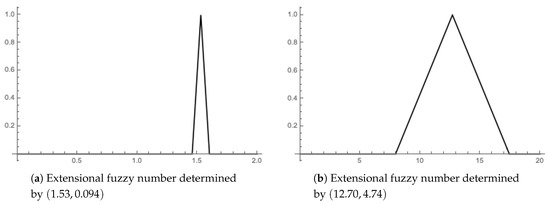
Figure 5. Extensional fuzzy numbers expressing the ice-cream sale “about $1.53$” and temperature “about $12.70$” in spring 2010.

To express weather conditions, for demonstration purposes, we will use the daily average temperatures (in degree Celsius) at Václav Havel Airport in Prague. Because each quarter contains approximately 90 records of temperature, and similarly to ice-cream sales, we summarize the temperature into an extensional fuzzy number determined by two parameters, namely the average temperature and the standard deviation in the quarter (see Table 2), which contains more information than only average temperature. Please note that the standard modeling of the relationship between temperatures and ice-cream sales (e.g., based on the interpolation or regression) use the average temperature in the quarters, while the random fluctuation of temperatures in the quarters expressed by the standard deviation is not considered (cf. [57]).

Table 2. Quarterly temperatures and standard deviations rounded to two decimals over 2008–2014.

	2008	2009	2010	2011	2012	2013	2014
$Q_1$	(3.11, 3.55)	(0.09, 4.44)	(−0.75, 5.63)	(0.94, 5.30)	(1.16, 6.95)	(−0.97, 4.04)	(3.44, 4.16)
$Q_2$	(13.37, 5.09)	(14.09, 3.22)	(12.70, 4.74)	(14.46, 4.37)	(13.94, 5.95)	(12.32, 5.59)	(13.19, 4.34)
$Q_3$	(16.53, 4.60)	(18.12, 2.96)	(17.02, 4.85)	(17.05, 3.26)	(17.40, 3.99)	(17.02, 4.64)	(17.05, 3.60)
$Q_4$	(4.75, 4.68)	(4.53, 8.81)	(2.13, 6.67)	(4.84, 4.54)	(3.96, 4.80)	(4.96, 4.53)	(6.35, 5.01)

An extensional fuzzy number expressing the temperature in a quarter and determined by parameters $(t,{\sigma }_t)$ is the fuzzy set $t_S:\mathbb{R}\to [0,1]$, which is defined in the same way as the similarity R for the quarterly sales. An example of the extensional fuzzy number expressing the temperature “about $12.7$” in spring 2010, which is determined by parameters $(12.70,4.74)$ in Table 2, is displayed in Figure 5b.

In the following subsection we will describe the procedure how to $\mathcal{S}$-interpolate extensional fuzzy numbers expressing temperatures and ice-cream sales in quarters in the years 2008–2014.

6.2. General Description of $\mathcal{S}$-Interpolation Procedure

Let $(x_{S_1}^1,y_{T_1}^1),\cdots ,(x_{S_n}^n,y_{T_n}^n)$ be pairs of extensional fuzzy numbers such that $x_{S_i}^i\le x_{S_{i+1}}^{i+1}$ for any $i=1,\cdots ,n$. We call these pairs of extensional fuzzy numbers as extensional fuzzy data. In contrast to the interpolation of real data, we must be more careful in the direct use of Formula (20) for extensional fuzzy data. The reason is that the fuzziness of extensional fuzzy numbers on input, which is expressed by a similarity relationship, is distributed through Formula (20) to another fuzziness specifying the similarity relation of extensional fuzzy number on the output of $\mathcal{S}$-interpolation. Since the input and output of extensional fuzzy data are in practice obtained by the measurement on different scales, the meanings of fuzziness are different for input and output fuzzy data, which leads to incorrect results by direct application of (20). In other words, unless the same measurement scale is used to determine the input and output fuzzy data, we cannot assume that extensional fuzzy data can be handled in one ordered MI-prefield, and the $\mathcal{S}$-interpolation introduced in Definition 14 cannot be applied for them. This problem can be overcome by a normalization procedure, which ensures that the normalized extensional fuzzy numbers will belong to the same ordered MI-prefield.

In what follows, we assume that extensional fuzzy data generally belong to ${\mathcal{F}}_{{\mathcal{S}}_I}\left(\mathbb{R}\right)\times {\mathcal{F}}_{{\mathcal{S}}_O}\left(\mathbb{R}\right)$, where ${\mathcal{F}}_{{\mathcal{S}}_I}\left(\mathbb{R}\right)$ and ${\mathcal{F}}_{{\mathcal{S}}_O}\left(\mathbb{R}\right)$ are ordered MI-prefields with a strongly compatible ${\mathcal{S}}_I$-ordering ${\le }_I$ and a strongly compatible ${\mathcal{S}}_O$-ordering ${\le }_O$. respectively. We use I and O in the indexes to refer to the input and output, respectively. Let ${\mathcal{F}}_{\mathcal{S}}\left(\mathbb{R}\right)$ be an ordered MI-prefield with a strongly compatible $\mathcal{S}$-orderings ≤, and let $N_I:{\mathcal{F}}_{{\mathcal{S}}_I}\left(\mathbb{R}\right)\to {\mathcal{F}}_{\mathcal{S}}\left(\mathbb{R}\right)$ and $N_O:{\mathcal{F}}_{{\mathcal{S}}_O}\left(\mathbb{R}\right)\to {\mathcal{F}}_{\mathcal{S}}\left(\mathbb{R}\right)$ be isomorphisms of ordered MI-prefields. We say that a pair $(N_I,N_O)$ of isomorphisms is a normalization of extensional fuzzy numbers if the composition $N_I^{-1}\circ N_O$ and $N_O^{-1}\circ N_I$ introduce natural correspondences between the ordered MI-prefields ${\mathcal{F}}_{{\mathcal{S}}_I}\left(\mathbb{R}\right)$ and ${\mathcal{F}}_{{\mathcal{S}}_O}\left(\mathbb{R}\right)$, i.e., $N_I^{-1}\circ N_0\left(x_S\right)$ is a natural image of $x_S$ in ${\mathcal{F}}_{{\mathcal{S}}_O}\left(\mathbb{R}\right)$ and vice versa $N_O^{-1}\circ N_I\left(y_T\right)$ is a natural image of $y_T$ in ${\mathcal{F}}_{{\mathcal{S}}_I}\left(\mathbb{R}\right)$. Please note that the decision if the compositions $N_I^{-1}\circ N_0$ and $N_I^{-1}\circ N_0$ are natural correspondences between the ordered MI-prefields ${\mathcal{F}}_{{\mathcal{S}}_I}\left(\mathbb{R}\right)$ and ${\mathcal{F}}_{{\mathcal{S}}_O}\left(\mathbb{R}\right)$ depends on the user. If ${\mathcal{F}}_{{\mathcal{S}}_I}\left(\mathbb{R}\right)={\mathcal{F}}_{{\mathcal{S}}_O}\left(\mathbb{R}\right)$, i.e., ${\mathcal{S}}_I={\mathcal{S}}_O=\mathcal{S}$, the pair $(N_I,N_O)$ given by $N_I=id=N_O$, where $id$ is the identity map on ${\mathcal{F}}_{\mathcal{S}}\left(\mathbb{R}\right)$, defines the trivial normalization of extensional fuzzy numbers, nevertheless, the user must agree that extensional fuzzy data are determined by the measurement on the same scale and thus can be processed in the same ordered MI-prefield ${\mathcal{F}}_{\mathcal{S}}\left(\mathbb{R}\right)$. Now, we can introduce the procedure of $\mathcal{S}$-interpolation of extensional fuzzy data.

Let $(x_{S_1}^1,y_{T_1}^1),\cdots ,(x_{S_n}^n,y_{T_n}^n)$ be extensional fuzzy data, and let $N_I:{\mathcal{F}}_{{\mathcal{S}}_I}\left(\mathbb{R}\right)\to {\mathcal{F}}_{\mathcal{S}}\left(\mathbb{R}\right)$ and $N_O:{\mathcal{F}}_{{\mathcal{S}}_O}\left(\mathbb{R}\right)\to {\mathcal{F}}_{\mathcal{S}}\left(\mathbb{R}\right)$ define a normalization of extensional fuzzy numbers. We put $x_S^{N_I}=N_I\left(x_S\right)$ and similarly $y_T^{N_O}=N_O\left(y_T\right)$. The procedure of linear $\mathcal{S}$-interpolation of extensional fuzzy data with respect to the normalization given by $(N_I,N_O)$ is as follows:

Input: 

extensional fuzzy number $x_S$ from ${\mathcal{F}}_{{\mathcal{S}}_I}\left(\mathbb{R}\right)$

Step 1: 

normalize $x_S$ with respect to $N_I$ to get $x_S^{N_I}$

Step 2: 

find $x_{S_i}^{i{N}_I},x_{S_{i+1}}^{i+1N_I}$ such that $x_{S_i}^{i{N}_I}\le x_S^{N_I}\le x_{S_{i+1}}^{i+1N_I}$

Step 3: 

compute $z_R$ from $(x_{S_i}^{i{N}_I},y_{T_i}^{i{N}_O})$ and $(x_{S_{i+1}}^{i+1N_I},y_{T_{i+1}}^{i+1N_O})$ by Formula (20)

Step 4: 

compute $y_T=N_O^{-1}\left(z_R\right)$ (a denormalization procedure)

Output: 

extensional fuzzy number $y_T$ from ${\mathcal{F}}_{{\mathcal{S}}_O}\left(\mathbb{R}\right)$

It is easy to see that if ${\mathcal{F}}_{{\mathcal{S}}_I}\left(\mathbb{R}\right)={\mathcal{F}}_{{\mathcal{S}}_O}\left(\mathbb{R}\right)$ and the input and output extensional fuzzy numbers were determined by the measurement on the same scale, one can set $(N_I,N_O)$ as the trivial normalization, and the output extensional fuzzy number coincides with the extensional fuzzy number obtained directly by Formula (20).

6.3. Experimental Results

Our extensional fuzzy data consist of 32 pairs $(t_{S_i}^i,s_{T_i}^i)$, where we put $i=1$ for winter 2008, $i=2$ for spring 2008, etc. Recall that each input extensional fuzzy number $t_{S_i}^i$ is determined by parameters $(t^i,{\sigma }_t^i)$ displayed in Table 2, where $t_i$ is the average temperature, ${\sigma }_i$ the standard deviation in the i-th quarter and $S_i$ is given by (21). For the output values, we will consider two situations:

(a)

the ice-cream sales are crisp fuzzy numbers, i.e., extensional fuzzy numbers $s_{T_i}^i$, where $T_i$ is the equality relation and only the first parameter in each pair $(s^i,{\sigma }_s^i)$ is considered in Table 1;

(b)

the ice-cream sales are “true” fuzzy numbers, i.e., extensional fuzzy numbers $s_{T_i}^i$, where the similarity $T_i$ is given by (21) and both parameters in each pair $(s^i,{\sigma }_s^i)$ are considered in Table 1.

The first situation is very common in practice and occurs when output data (ice-cream sales) are available as real numbers, and we have no further information. The second situation requires additional information, for example, quarterly sales are average ice-cream sales that are calculated from weekly sales in quarters, where the standard deviation provides additional information, or the expert expresses an inaccuracy in the total sale in the quarter.

Let ${\mathcal{F}}_{{\mathcal{S}}_{\infty }}\left(\mathbb{R}\right)$ be the ordered MI-prefield introduced in Example 12. Obviously, our extensional fuzzy data belong to ${\mathcal{F}}_{{\mathcal{S}}_{\infty }}{\left(\mathbb{R}\right)}^2$, where $p_i$ is the inverse element to the standard deviation ${\sigma }_i$, i.e., $p_i=\frac{1}{{\sigma }_i}$, but the input and output extensional fuzzy numbers cannot be reasonably processed in this ordered MI-prefield without normalization. Indeed, the scale for measuring temperature is different from the scale used for sales of ice-cream, and even scales within different quarters are different as could be seen from Table 3, where we display the standard deviations for the temperatures and ice-cream sales.

Table 3. Data for normalization computed in quarters 2008–2017.

Quarters	Temperature st. Deviation $\left({\mathit{\sigma }}_{\mathit{t},\mathit{j}}\right)$	Ice-Cream Sale st. Deviation $\left({\mathit{\sigma }}_{\mathit{s},\mathit{j}}\right)$
$Q_1$	8.110	0.036
$Q_2$	8.063	0.010
$Q_3$	8.161	0.313
$Q_4$	8.034	0.072

In contrast to the standard deviations of temperature in quarters (the standard deviation for all temperatures in 2008–2014 is $8.17$), which are almost the same, there are large differences between the standard deviations of ice-cream sales in quarters (the standard deviation for all sales in 2008–2014 is $1.02$). The variability of the standard deviations of ice-cream sales forces us to model the relationship between temperature and ice-cream sales in each quarter separately, otherwise the resulting sales uncertainty may be affected by inaccurate normalization. This would certainly happen if we applied overall normalization to all sales. Therefore, before we use the linear $\mathcal{S}$-interpolation procedure introduced in the previous subsection, we normalize the standard deviations with respect to the standard deviations of the temperatures and the sales in the respective quarters of the years 2008–2014, see Table 3. Please note that the normalized values (i.e., standard deviations) are measured in the unit of the standard deviation.

For any extensional fuzzy number $t_{S_p}$ expressing a temperature in a quarter $Q_j$ ($j=1,\cdots ,4)$, we define $N_{I,j}\left(t_{S_p}\right)=t_{S_{p^{\prime }}}$ with $p^{\prime }=p·{\sigma }_{t,j}$, where ${\sigma }_{t,j}$ is the standard deviation of temperatures in $Q_j$. Similarly, for any extensional fuzzy number $s_{T_q}$ expressing an ice-cream sale in a quarter $Q_j$, we define $N_{O,j}\left(s_{T_q}\right)=s_{T_{q^{\prime }}}$ with $q^{\prime }=q·{\sigma }_{s,j}$, where ${\sigma }_{s,j}$ is the standard deviation of sales in $Q_j$. For $p=q=\infty$, we put $p^{\prime }=q^{\prime }=\infty ·{\sigma }_t=\infty ·{\sigma }_s=\infty$, hence, $N_{I,j}\left(t_{S_{\infty }}\right)=t_{S_{\infty }}$ and $N_{O,j}\left(s_{T_{\infty }}\right)=s_{T_{\infty }}$. Please note that $p^{\prime }=p·{\sigma }_{t,j}$ (and similarly $q^{\prime }=a·{\sigma }_{s,j}$) is derived from the following formula

$$\begin{array}{c}\frac{1}{p^{\prime }}=\frac{\frac{1}{p}}{{\sigma }_t^j}\end{array}$$

where $\frac{1}{p}$ represents a standard deviation for p and $\frac{1}{p^{\prime }}$ a standard deviation for $p^{\prime }$, and thus the standard deviation $\frac{1}{p^{\prime }}$ is a normalization of the standard deviation $\frac{1}{p}$ with respect to ${\sigma }_{t,j}$. According to Example 13, the maps $N_{I,j}$ and $N_{O,j}$ are isomorphisms from ${\mathcal{F}}_{{\mathcal{S}}_{\infty }}\left(\mathbb{R}\right)$ onto ${\mathcal{F}}_{{\mathcal{S}}_{\infty }}\left(\mathbb{R}\right)$. In addition, we agree that these isomorphisms are appropriately selected for normalization, where we do not measure in the original units, which are clearly different, but in the units of standard deviations in quarters, which are abstract and the same for input and output.

Unlike the standard linear interpolation, we cannot display the linear $\mathcal{S}$-interpolation in a clear way, because we have infinitely many extensional fuzzy numbers for any real number. On Figure 6, we illustrate the linear $\mathcal{S}$-interpolation on extensional fuzzy data observed in summer that are crisp and fuzzy, and we show separately the use of each rule of Formula (20) from Definition 15, where the computational algorithm is designed according to the procedure established in the previous subsection. In Figure 6a-left, the temperature measured as “about 17.7” and expressed by the extensional fuzzy number $t_{S_p}$ with $t=17.7$ and $p=1/4$ (or ${\sigma }_t=4$) gives the estimation of ice-cream sale $s_{T_q}$ with $s=2.857$ and $q=1/0.153$ (or ${\sigma }_s=0.153$). Since the sales of ice-cream in output data are crisp numbers, the uncertainty of the estimated sale is only affected by the uncertainty of the input data temperatures and the uncertainty of the temperature for which the sale is estimated. The standard deviation ${\sigma }_{t,3}=8.161$ for normalization and ${\sigma }_{s,3}=0.313$ for denormalization are used in our procedure to get an appropriate estimation of the uncertainty of the ice-cream sale. In Figure 6a-right, we consider the same input data as above, but the sales of ice-cream in output data are “true” extensional fuzzy numbers. It can be seen that in both situations the same estimate of ice-cream sales is obtained, which indicates a dominant similarity among the used temperatures. In other words, the uncertainty present in the sales nodes is lower than the uncertainty present in a used temperature. In Figure 6b-left, the input temperature determined as “about $17.4$” and expressed by $t_{S_p}$ with $t=17.4$ and $p=1/3$ (or ${\sigma }_t=3$) gives the estimation of ice-cream sale that coincides with the crisp sale output $2.57$ for the temperature node $t_{S_{p_{19}}}^{19}$ with $t^{19}=17.4$ and $p_{19}=1/3.99$ (or ${\sigma }_{t^{19}}=3.99)$. The reason is that $t=t^{19}$ and simultaneously $S_p\le S_{p_{19}}$ (i.e., $p=1/3>1/3.99=p_{19}$), and due to the uncertainty monotonicity condition (19), the uncertainty of ice-cream sale corresponding to temperature $t_{S_p}$ cannot be higher than the uncertainty of output corresponding to temperature node $t_{S_{p_{19}}}^{19}$. Similarly, in Figure 6b-right, the estimation of ice-cream sale coincides with the sale output $s_{T_{q_{19}}}^{19}$ with $s^{19}=2.57$ and $q_{19}=1/0.204$ (or ${\sigma }_{s^{19}}=0.204$). On the other side, in Figure 6c-left, the input temperature determined as “about 17.4” and expressed by $t_{S_p}$ with $t=17.4$ and $p=1/4.3$ (or ${\sigma }_t=4.3$) gives the estimation of ice-cream sale $s_{T_q}$ with $s=s^{19}=2.57$ and $q=1/0.165$ (or ${\sigma }_q=0.165$). The reason is that $t=t^{19}$ and simultaneously $S_p>S_{p_{19}}$ and therefore, the uncertainty of ice-cream sale output corresponding to temperature $t_{S_p}$ can be higher than the uncertain of output corresponding to temperature node $t_{S_{p_{19}}}^{19}$ (i.e., $p_{19}=1/3.99>1/4.3=p$), which results in the application of Formula (18). In Figure 6c-right, we display the resulting estimation of ice-cream sale in the situation when the input data are the same as above and the ice-cream sales in the output data are expressed by extensional fuzzy numbers. One can see that the estimation is the same as for sales expressed in real numbers, which indicates a dominant similarity among the used temperatures similarly as in Figure 6a.

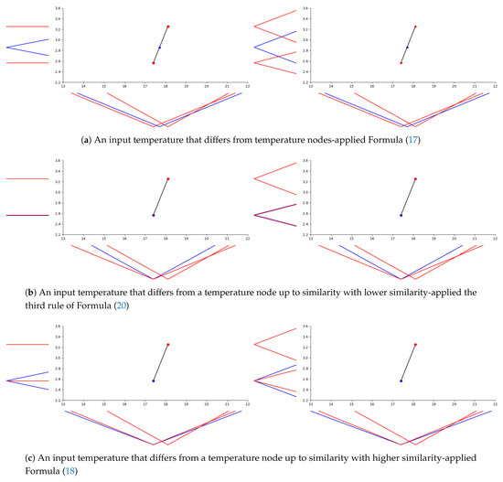
Figure 6. Estimation of ice-cream sales based on the linear $\mathcal{S}$-interpolation for selected temperatures in summer, where sale data are crisp (left) and fuzzy (right); temperature and ice-cream sale nodes are colored red, the selected (input) temperature and estimated (output) sale blue.

In Figure 7, we illustrate the linear $\mathcal{S}$-interpolation between three pairs of temperatures and ice-cream sales observed in winter, where sales are expressed by extensional fuzzy numbers, and show the estimation of ice-cream sales for three selected temperatures. Two of them, namely “about 1.7” (${\sigma }_{t_1}=3$) and “about 3.3” (${\sigma }_{t_2}=4.5$), lie between temperature nodes and “about 1.16” (${\sigma }_{t_3}=7.35$) coincides with the first node up to similarity with a higher similarity. The estimation of ice-cream sales is “about 0.257” (${\sigma }_{s_1}=0.032$), “about 0.277” (${\sigma }_{s_2}=0.029$) and “about 0.266” (${\sigma }_{s_3}=0.033$).

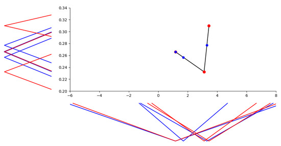
Figure 7. Estimation of ice-cream sales based on the linear $\mathcal{S}$-interpolation for selected temperatures in winter.

It should be noted that in practice it is very difficult to predict the average temperature in the coming quarter as a single number and it is more appropriate to use a confidence interval or an extensional fuzzy number as in our case. The linear $\mathcal{S}$-interpolation can be then used to predict ice-cream sales in the coming quarter, providing important information for production planning.

6.4. Comparing with Other Approaches—Discussion

As stated in the Introduction, fuzzy interpolation is a rather old problem with many well-developed techniques, no matter we talk about the geometrically motivated or rather logically motivated approaches. Thus, the formal apparatus designed in this article should naturally face some comparison with them. In data sciences (e.g., in pattern recognition or classification), we usually encounter an exhaustive experimental comparison with some objective evaluation on a given cost function. However, up to our best knowledge, there is no generally accepted quality criterion determining for fuzzy interpolation tasks. Indeed, there is always a way to define such a criterion, but it would be purely subjectively designed.

In such a case, we opt for a demonstrative comparison on the above-presented ice-cream sales data with two prototypical representatives of existing methods employing different paradigms. The first one that stems from the geometric motivation is the well-known Kóczy–Hirota (abbr. KH) methods introduced in [9]. Although this method is rather old and several improvements have been employed soon after its publication, it is a fundamental basis for many other geometrically oriented techniques, see [58]. Moreover, this method possesses the advantage of low computational costs and it is driven by the same crisp technique—the classical linear interpolation. For observing the differences, we find this choice very appropriate.

The second method stems from the logical (approximate reasoning) motivation and it is the standard fuzzy relational inference. Such method models the existing rules by a fuzzy relation that is either conjunctive (often called Mamdani–Assilian [59]) or implicative [60] and connects the fuzzy relation to a composition-based inference, i.e., to an appropriate image of a fuzzy set under the fuzzy relation. For more details on the distinct types of rules, their properties and the connection to the compositions/images as inference mechanisms, we refer to [61,62]. Briefly, the appropriate combinations are: (1) the implicative fuzzy rule base (antecedents and consequents are connected via a residated implication, rules are aggregated with help of the minimum) together with the basic composition, which is the well-known Compositional Rule of Inference (CRI); and (2) the conjunctive fuzzy rule base (antecedents and consequents are connected via a t-norm, rules are aggregated with help of the maximum) together with the Bandler–Kohout subproduct. The opposite combinations may cause complications, see [63].

Remark 10.

Many articles use the combination of the (Mamdani–Assilian) conjunctive fuzzy rules base and the CRI. This is often totally correct as the vast majority of cases deals with crisp inputs while the danger appears in the case of fuzzy inputs. Indeed, in the case of crisp inputs, no matter we deal with CRI or the Bandler–Kohout subproduct, the inference degenerates into a simple substitution of the crisp input into the given fuzzy relation so, we even cannot distinguish between these two compositional inferences, they coincide. But for the fuzzy interpolation task with fuzzy inputs, the choice of the combination is essential.

Now, let us focus on several examples from the above elaborated ice-cream sales dataset. The first example considers “the simplest” case when the antecedents as well as consequents are ordered with respect to the interval-ordering of $\alpha$-cuts and the fuzzy input lies “between” the antecedents, and the antecedents as well as consequents are overlapping. This case is demonstrated on a part of the autumn data from the ice-cream sales problem, see Figure 8. As we can see, the KH method and the proposed $\mathcal{S}$-interpolation method provides very comparable results. The proposed method generated a bit narrower output however, this advantage is caused by a well-chosen relativization determined by the standard deviation transformation caused and indeed, it could be easily lost. Therefore, we do not dare to claim it as a generally valid principle. The third method determined by fuzzy relational inference determined something that is logically correct however, not meeting the expectations of the analytical interpolation that is used under the implicit assumption of the satisfaction of the functionality axiom. Please note that the choice of the algebra has no significant influence, for example, using the Łukasiewicz implications would lead to a higher output fuzzy set but still reaching values around 0.6 at maximum and moreover, with an unlimited support. Here, we would like to emphasize that this is nothing against fuzzy relational inference. The problem lies in the fact that the antecedents are closer to each other than the consequents and thus, the fuzzy rule base is not coherent [64] which is a sort of consistency (non-conflictness) of the fuzzy rules. In other words, this means nothing wrong about fuzzy relational inference but rather about its non-applicability on such interpolative setting. Finally, the use of the other preferred combination (Mamdani–Assilian rules with Bandler–Kohout subproduct) would lead to a subnormal and non-convex output fuzzy set—again not meeting the implicit functionality axiom.

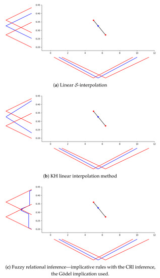
Figure 8. Comparison of our method with two fundamental interpolation techniques on particular part of autumn ice-cream sales.

Now, let us consider the cases depicted on the right-hand side of Figure 6a. There, the antecedents are not ordered with respect to the interval-ordering of $\alpha$-cuts which makes impossible to use the KH method (at least in its original form) while the proposed $\mathcal{S}$-interpolation works well due to the robustness of the $\mathcal{S}$-ordering. The fuzzy relational inference here can easily infer the outputs too as the ordering of antecedents does not play any role. However, the consequent part makes the inferred outputs inappropriate, in particular, the disjointness of the consequents is an extreme version of the incoherence and thus, the implicative rules would infer a fuzzy set equal to zero on the whole universe. For the completeness, let us mention that the Mamdani–Assilian rules would result again subnormal and non-convex outputs without any functional meaning.

Another similar example is depicted on the right-hand side of Figure 6b. It is the same situation as in the previous case with the only difference that the fuzzy input is located in one of the nodes for the antecedents; however, the input is narrower than the antecedent. The figure shows how the proposed $\mathcal{S}$-interpolation generates the outputs while up to our best knowledge, KH method would not be applicable. But again, after some adjustments, KH method would deal with this input too and infer some reasonable output. The fuzzy relational inference would lead to the same as in the previous case.

The last case we consider is the situation of a sparse rule base where fuzzy relational inference would not again meet the expectations imposed by the assumed functionality axiom. In particular, if we were given two disjoint antecedents and the fuzzy input would be placed in between of them in such a way it would be disjoint with both, the inferred output would be equal to 1 on the whole output universe (or to 0, in the case of the Mamdani–Assilian rules with the Bandler–Kohout subproduct). Here, we would like to again emphasize that this not wrong at all from the logical perspective. If the rules are logical constraints stating that the consequent should be inferred under the assumption that the antecedent holds, and none of the antecedent is met by the input, we may deduce nothing, which is mirrored by the outputs 1 or 0, depending on the semantics of the rules. This is only again a case where, without further improvement like the one proposed in [15], relational inference is not appropriate for approximate reasoning schemes of this type of sparse cases. Here, the KH method performs a practical advantage as it is deliberately designed for the sparse rule bases. This case is not demonstrated on the real data as such a case has not occurred in the ice-cream sales dataset at all. However, from the principal point of view, the results obtained from the KH method and from the proposed $\mathcal{S}$-interpolation would be very comparable—mimicking the cases depicted in Figure 8.

7. Conclusions and Future Work

The presented approach stemmed from the particular fuzzy arithmetic, namely from the arithmetic of extensional fuzzy numbers [19,25]. The first steps from the arithmetic towards the ordering were published in [23,24] with the aim to construct metrics of fuzzy numbers [48]. The original motivation came from the need for modeling the triangle inequality in the metric-like structures. However, it is clear that the importance of $\mathcal{S}$-orderings is much only higher and mainly more general. Apart from the clear directions coming from the mathematical analysis based on the extensional fuzzy numbers (fuzzy approximation, mathematical analysis, construction of limits, convergences), already [24] mentioned approximate reasoning as one of the related areas where this research can have an importance.

Indeed, the fuzzy interpolation is one of the crucial problems in approximate reasoning and it is not possible to study it from the analytical point of view if we cannot order the used fuzzy sets (fuzzy numbers) in such a way to be able to state that an input lies “between two given fuzzy nodes”. This article copes with this topic and incorporates the technique of the $\mathcal{S}$-interpolation generically from the formal roots (arithmetic, ordering, $\mathcal{S}$-functions) to the problem formalization ($\mathcal{S}$-interpolation, uncertainty monotonicity, and standard monotonicity) towards the practical implementation and the demonstrative example. It is clear that the proposed calculation is just one of the rich pool of possibilities and as mentioned in Remark 9 other techniques can be introduced analogously. The remark also contains a discussion pointing the potential drawbacks of more sophisticated approaches as well as the direction towards their elimination.

One can view the proposed approach as a single instance of more general classes of $\mathcal{S}$-interpolations not only form the linear, polynomial or other basis point of view, but also form the point of view of processing the vagueness. Indeed, following the arithmetic of extensional fuzzy numbers, also the $\mathcal{S}$-interpolation is a sort of two-step procedure. In the first one, the “crisp” part of the task is solved using the standard technique. In the second one, the resulting vagueness (uncertainty, tolerance, etc.) is calculated as a result of the computation with the similarities entering the interpolation problem. And as one can modify the first step of the procedure and consider, e.g., polynomial interpolations, the second step can be modified as well, and the resulting similarity may be deduced differently. So far, the procedure coming from the arithmetic of extensional numbers was naturally inherited as the linear $\mathcal{S}$-interpolation is derived from the arithmetic operations. However, considering the definition of the $\mathcal{S}$-function that is more general and the above-introduced examples (exponential, logarithmic, trigonometric), we are equipped with tools that allow modeling of the spreading of the vagueness in distinct ways according to the application or theoretical needs.

In our future research we plan to continue in the development of $\mathcal{S}$-interpolation for other types of functions and using metrics introduced in [48] we want to design more advanced interpolation approaches. For example, motivated by the Gaussian process regression (kriging) that has become popular in Machine Learning [65], where the interpolated values are modeled by Gaussian processes and are basically obtained as weighted averages of known neighbor nodes (see, e.g., [66]). In addition, it is a very challenging task to design an interpolation (regression) model that together admits probability and fuzziness of the data. The proposed theory seems to provide promising tools for successful solutions of this task.

References

- Perfilieva, I. Finitary Solvability Conditions for Systems of Fuzzy Relation Equations. Inf. Sci. 2013, 234, 29–43. [Google Scholar] [CrossRef]
- Di Nola, A.; Sessa, S.; Pedrycz, W.; Sanchez, E. Fuzzy Relation Equations and Their Applications to Knowledge Engineering; Kluwer: Boston, MA, USA, 1989. [Google Scholar]
- Pedrycz, W. Applications of fuzzy relational equations for methods of reasoning in presence of fuzzy data. Fuzzy Sets Syst. 1985, 16, 163–175. [Google Scholar] [CrossRef]
- De Baets, B. Analytical solution methods for fuzzy relational equations. In The Handbook of Fuzzy Set Series Vol. 1; Dubois, D., Prade, H., Eds.; Academic Kluwer Publ.: Boston, MA, USA, 2000; pp. 291–340. [Google Scholar]
- Perfilieva, I.; Lehmke, S. Correct models of fuzzy IF-THEN rules are continuous. Fuzzy Sets Syst. 2006, 157, 3188–3197. [Google Scholar] [CrossRef]
- Cornejo, M.E.; Lobo, D.; Medina, J. On the solvability of bipolar max-product fuzzy relation equations with the product negation. J. Comput. Appl. Math. 2018, 354, 520–532. [Google Scholar] [CrossRef]
- Štěpnička, M.; De Baets, B. Interpolativity of at-least and at-most models of monotone single-input single-output fuzzy rule bases. Inf. Sci. 2013, 234, 16–28. [Google Scholar] [CrossRef]
- Štěpnička, M.; Jayaram, B. Interpolativity of at-least and at-most models of monotone fuzzy rule bases with multiple antecedent variables. Fuzzy Sets Syst. 2016, 297, 26–45. [Google Scholar] [CrossRef]
- Kóczy, L.; Hirota, K. Approximate reasoning by linear rule interpolation and general approximation. Int. J. Approx. Reason. 1993, 9, 197–225. [Google Scholar] [CrossRef]
- Vetterlein, T.; Štěpnička, M. Completing fuzzy if-then rule bases by means of smoothing. Int. J. Uncertain. Fuzziness Knowl.-Based Syst. 2006, 14, 235–244. [Google Scholar] [CrossRef]
- Kóczy, L.; Hirota, K. Interpolative reasoning with insufficient evidence in sparse fuzzy rule bases. Inf. Sci. 1993, 71, 169–201. [Google Scholar] [CrossRef]
- Baranyi, P.; Kóczy, L.; Gedeon, T. A generalized concept for fuzzy rule interpolation. IEEE Trans. Fuzzy Syst. 2004, 12, 820–837. [Google Scholar] [CrossRef]
- Li, F.; Shang, C.; Li, Y.; Yang, J.; Shen, Q. Interpolation with Just Two Nearest Neighboring Weighted Fuzzy Rules. IEEE Trans. Fuzzy Syst. 2020, 28, 2255–2262. [Google Scholar] [CrossRef]
- Bouchon-Meunier, B.; Dubois, D.; Marsala, C.; Prade, H.; Ughetto, L. A comparative view of interpolation methods between sparse fuzzy rules. In Proceedings of the Annual Conference of the North American Fuzzy Information Processing Society-NAFIPS, Vancouver, BC, Canada, 25–28 July 2001; Volume 5, pp. 2499–2504. [Google Scholar]
- Perfilieva, I.; Dubois, D.; Prade, H.; Esteva, F.; Godo, L.; Hoďáková, P. Interpolation of fuzzy data: Analytical approach and overview. Fuzzy Sets Syst. 2012, 192, 134–158. [Google Scholar] [CrossRef]
- Mareš, M. Computation over Fuzzy Quantities; CRC Press: Boca Raton, FL, USA, 1994. [Google Scholar]
- Bělohlávek, R. Fuzzy Relational Systems: Foundations and Principles; Kluwer Academic, Plenum Press: Dordrecht, the Netherlands; New York, NY, USA, 2002. [Google Scholar]
- Klawonn, F. Fuzzy Points, Fuzzy Relations and Fuzzy Functions. In Discovering the World with Fuzzy Logic; Novák, V., Perfilieva, I., Eds.; Springer: Berlin, Germany, 2000; pp. 431–453. [Google Scholar]
- Holčapek, M.; Štěpnička, M. MI-algebras: A new framework for arithmetics of (extensional) fuzzy numbers. Fuzzy Sets Syst. 2014, 257, 102–131. [Google Scholar] [CrossRef]
- Dubois, D.; Prade, H. Operations on fuzzy numbers. Int. J. Syst. Sci. 1978, 9, 613–626. [Google Scholar] [CrossRef]
- Stefanini, L.; Sorini, L.; Guerra, M. Parametric representation of fuzzy numbers and application to fuzzy calculus. Fuzzy Sets Syst. 2006, 157, 2423–2455. [Google Scholar] [CrossRef]
- Mareš, M. Weak arithmetics of fuzzy numbers. Fuzzy Sets Syst. 1997, 91, 143–153. [Google Scholar] [CrossRef]
- Štěpnička, M.; Holčapek, M.; Škorupová, N. Orderings of Extensional Fuzzy Numbers. In Proceedings of the IEEE International Conference on Fuzzy Systems (FUZZ-IEEE) 2019, New Orleans, LA, USA, 23–26 June 2019. [Google Scholar]
- Štěpnička, M.; Škorupová, N.; Holčapek, M. On the properties of orderings of extensional fuzzy numbers. In Proceedings of the IEEE International Conference on Fuzzy Systems (FUZZ-IEEE) 2020, Glasgow, UK, 19–24 July 2020. [Google Scholar]
- Holčapek, M.; Štěpnička, M. Arithmetics of extensional fuzzy numbers–part I: Introduction. In Proceedings of the IEEE International Conference on Fuzzy Systems, Brisbane, Australia, 10–15 June 2012. [Google Scholar]
- Holčapek, M.; Štěpnička, M. Arithmetics of extensional fuzzy numbers–part II: Algebraic framework. In Proceedings of the IEEE International Conference on Fuzzy Systems, Brisbane, Australia, 10–15 June 2012. [Google Scholar]
- Ma, M.; Friedman, M.; Kandel, A. A new fuzzy arithmetic. Fuzzy Sets Syst. 1999, 108, 83–90. [Google Scholar] [CrossRef]
- Stefanini, L.; Sorini, L.; Guerra, M. Simulation of fuzzy dynamical systems using the LU-representation of fuzzy numbers. Chaos Solitons Fractals 2006, 29, 638–652. [Google Scholar] [CrossRef]
- Fortin, J.; Dubois, D.; Fargier, H. Gradual Numbers and Their Application to Fuzzy Interval Analysis. IEEE Trans. Fuzzy Syst. 2008, 16, 388–402. [Google Scholar] [CrossRef]
- Boixader, D.; Jacas, J. Extensionality based approximate reasoning. Int. J. Approx. Reason. 1998, 19, 221–230. [Google Scholar] [CrossRef]
- Klawonn, F.; Castro, J.L. Similarity in Fuzzy Reasoning. Mathw. Soft Comput. 1995, 2, 197–228. [Google Scholar]
- Klawonn, F.; Kruse, R. Equality relations as a basis for fuzzy control. Fuzzy Sets Syst. 1993, 54, 147–156. [Google Scholar] [CrossRef]
- Holčapek, M.; Wrublová, M.; Bacovský, M. Quotient MI-groups. Fuzzy Sets Syst. 2016, 283, 1–25. [Google Scholar] [CrossRef]
- Holčapek, M. On generalized quotient MI-groups. Fuzzy Sets Syst. 2017, 326, 3–23. [Google Scholar] [CrossRef]
- Holčapek, M.; Škorupová, N. Topological MI-Groups: Initial Study. In IPMU 2018: Information Processing and Management of Uncertainty in Knowledge-Based Systems, Proceedings of the Applications-17th International Conference, Cádiz, Spain, 11–15 June 2018; Proceedings, Part III; Medina, J., Ojeda-Aciego, M., Galdeano, J.L.V., Perfilieva, I., Bouchon-Meunier, B., Yager, R.R., Eds.; Springer: Berlin/Heidelberg, Germany, 2018; Volume 855, Communications in Computer and Information Science; pp. 603–615. [Google Scholar]
- Aryal, B.; Bokati, L.; Godinez, K.; Ibarra, S.; Liu, H.; Wang, B.; Kreinovich, V. Common Sense Addition Explained by Hurwicz Optimism-Pessimism Criterion. J. Uncertain Syst. 2019, 13, 171–174. [Google Scholar]
- Hurwicz, L. Optimality Criteria for Decision Making Under Ignorance; Cowles Commission Discussion Paper, Statistics; Yale University: New Haven, CT, USA, 1951; pp. 171–174. [Google Scholar]
- Zadeh, L. Similarity relations and fuzzy orderings. Inf. Sci. 1971, 3, 177–200. [Google Scholar] [CrossRef]
- Bodenhofer, U. A Similarity-Based Generalization of Fuzzy Orderings Preserving the Classical Axioms. Int. J. Uncertain. Fuzziness Knowl.-Based Syst. 2000, 8, 593–610. [Google Scholar] [CrossRef]
- Wang, W.; Wang, Z. Total orderings defined on the set of all fuzzy numbers. Fuzzy Sets Syst. 2014, 243, 131–141. [Google Scholar] [CrossRef]
- Asady, B.; Zendehnam, A. Ranking fuzzy numbers by distance minimization. Appl. Math. Model. 2007, 31, 2589–2598. [Google Scholar] [CrossRef]
- De Hierro, A.F.R.L.; Roldán, C.; Herrera, F. On a new methodology for ranking fuzzy numbers and its application to real economic data. Fuzzy Sets Syst. 2018, 353, 86–110. [Google Scholar] [CrossRef]
- Van Broekhoven, E.; De Baets, B. A linguistic fuzzy model with a monotone rule base is not always monotone. In Proceedings of the EUSFLAT-LFA’05, Barcelona, Spain, 7–9 September 2005; pp. 530–535. [Google Scholar]
- Van Broekhoven, E.; De Baets, B. On the monotonicity of Mamdani-Assilian models with two input variables. In Proceedings of the NAFIPS’06, Montreal, QC, Canada, 3–6 June 2006; pp. 102–107. [Google Scholar]
- Štěpnička, M.; De Baets, B. Implication-based models of monotone fuzzy rule bases. Fuzzy Sets Syst. 2013, 232, 134–155. [Google Scholar] [CrossRef]
- Bodenhofer, U. Orderings of Fuzzy Sets Based on Fuzzy Orderings Part I: The Basic Approach. Mathw. Soft Comput. 2008, 15, 201–218. [Google Scholar]
- Bodenhofer, U. Orderings of Fuzzy Sets Based on Fuzzy Orderings Part II: Generalizations. Mathw. Soft Comput. 2008, 15, 219–249. [Google Scholar]
- Štěpnička, M.; Škorupová, N.; Holčapek, M. From arithmetics of extensional fuzzy numbers to their distances. In Proceedings of the IEEE International Conference on Fuzzy Systems (FUZZ-IEEE) 2020, Glasgow, UK, 19–24 July 2020. [Google Scholar]
- Wang, X.; Kerre, E.E. Reasonable properties for the ordering of fuzzy quantities (I). Fuzzy Sets Syst. 2001, 118, 375–385. [Google Scholar] [CrossRef]
- Wang, X.; Kerre, E.E. Reasonable properties for the ordering of fuzzy quantities (II). Fuzzy Sets Syst. 2001, 118, 387–405. [Google Scholar] [CrossRef]
- Van Broekhoven, E.; De Baets, B. Monotone Mamdani-Assilian models under mean of maxima defuzzification. Fuzzy Sets Syst. 2008, 159, 2819–2844. [Google Scholar] [CrossRef]
- Van Broekhoven, E.; De Baets, B. Only smooth rule bases can generate monotone Mamdani-Assilian models under Center-of-gravity defuzzification. IEEE Trans. Fuzzy Syst. 2009, 17, 1157–1174. [Google Scholar] [CrossRef]
- Štěpnička, M.; De Baets, B. Monotonicity of implicative fuzzy models. In Proceedings of the FUZZ-IEEE 2010, Barcelona, Spain, 18–23 July 2010; pp. 2334–2340. [Google Scholar]
- Mandal, S.; Jayaram, B. Monotonicity of SISO Fuzzy Relational Inference With an Implicative Rule Base. IEEE Trans. Fuzzy Syst. 2016, 24, 1475–1487. [Google Scholar] [CrossRef]
- Bodenhofer, U.; De Cock, M.; Kerre, E.E. Openings and closures of fuzzy preorderings: Theoretical basics and applications to fuzzy rule-based systems. Int. J. Gen. Syst. 2003, 32, 343–360. [Google Scholar] [CrossRef]
- Bodenhofer, U.; Bauer, P. Interpretability of Linguistic Variables: A Formal Account. Kybernetika 2005, 41, 227–248. [Google Scholar]
- Dvořáčková, H.; A., K.; Tichý, T. Sales Prediction in the Ice Category Applying Fuzzy Sets Theory. Ekon. Rev. Cent. Eur. Rev. Econ. Issues 2018, 21, 35–41. [Google Scholar]
- Das, S.; Chakraborty, D.; Kóczy, L. Linear fuzzy rule base interpolation using fuzzy geometry. Int. J. Approx. Reason. 2019, 112, 105–118. [Google Scholar] [CrossRef]
- Mamdani, E.H.; Assilian, S. An experiment in linguistic synthesis with a fuzzy logic controller. Int. J. Man-Mach. Stud. 1975, 7, 1–13. [Google Scholar] [CrossRef]
- Jones, H.; Charnomordic, B.; Dubois, D.; Guillaume, S. Practical inference with systems of gradual implicative rules. IEEE Trans. Fuzzy Syst. 2009, 17, 61–78. [Google Scholar] [CrossRef]
- Dubois, D.; Prade, H. What are fuzzy rules and how to use them. Fuzzy Sets Syst. 1996, 84, 169–185. [Google Scholar] [CrossRef]
- Štěpnička, M.; Mandal, S. Fuzzy inference systems preserving Moser–Navara axioms. Fuzzy Sets Syst. 2018, 338, 97–116. [Google Scholar] [CrossRef]
- Štěpnička, M.; Jayaram, B.; Su, Y. A short note on fuzzy relational inference systems. Fuzzy Sets Syst. 2018, 338, 90–96. [Google Scholar] [CrossRef]
- Dubois, D.; Prade, H.; Ughetto, L. Checking the Coherence and Redundancy of Fuzzy Knowledge Bases. IEEE Trans. Fuzzy Syst. 1997, 5, 398–417. [Google Scholar] [CrossRef]
- Rasmussen, C.; Williams, C. Gaussian Processes for Machine Learning; The MIT Press: Cambridge, MA, USA, 2006. [Google Scholar]
- Le, N.D.; Zidek, J.V. Statistical Analysis of Environmental Space-Time Processes; Springer: New York, NY, USA, 2006. [Google Scholar]
Publisher’s Note: MDPI stays neutral with regard to jurisdictional claims in published maps and institutional affiliations. |
© 2021 by the authors. Licensee MDPI, Basel, Switzerland. This article is an open access article distributed under the terms and conditions of the Creative Commons Attribution (CC BY) license (http://creativecommons.org/licenses/by/4.0/).