On the Semi-Analytical Solutions in Hydrodynamics of Ideal Fluid Flows Governed by Large-Scale Coherent Structures of Spiral-Type

Abstract

We have presented here a clearly formulated algorithm or semi-analytical solving procedure for obtaining or tracing approximate hydrodynamical fields of flows (and thus, videlicet, their trajectories) for ideal incompressible fluids governed by external large-scale coherent structures of spiral-type, which can be recognized as special invariant at symmetry reduction. Examples of such structures are widely presented in nature in “wind-water-coastline” interactions during a long-time period. Our suggested mathematical approach has obvious practical meaning as tracing process of formation of the paths or trajectories for material flows of fallout descending near ocean coastlines which are forming its geometry or bottom surface of the ocean. In our presentation, we explore (as first approximation) the case of non-stationary flows of Euler equations for incompressible fluids, which should conserve the Bernoulli-function as being invariant for the aforementioned system. The current research assumes approximated solution (with numerical findings), which stems from presenting the Euler equations in a special form with a partial type of approximated components of vortex field in a fluid. Conditions and restrictions for the existence of the 2D and 3D non-stationary solutions of the aforementioned type have been formulated as well.

1. Introduction, Equations of Motion

A lot of meaningful works in the field of hydrodynamics are devoted to investigations of influencing large-scale coherent structures on averaged fluid flows which take place on a bay or ocean coastline in a sufficiently stable regime [1,2,3]. Such research is known to have duly practical meaning with aim of tracing paths or trajectories of material flows of fallout descending near ocean coastlines which are forming its structure, topology of the bottom surface of the ocean and thus, e.g., let us predict and trace the safe ways of ships floating near aforementioned coastline or reefs.

In the current research, we will use Euler full equations for incompressible flow for the modelling of such structure or solutions for ideal fluid flows. In accordance with [4,5], the Euler system of equations governs flows of incompressible non-viscous fluid to be presented in the Cartesian coordinates as follows (under the given initial or boundary conditions):

$$\nabla \cdot \overrightarrow{u} = 0 ,$$

(1)

$$\frac{\partial \overrightarrow{u}}{\partial t} + (\overrightarrow{u} \cdot \nabla ) \overrightarrow{u} = -\frac{\nabla p}{\rho } + \overrightarrow{F} ,$$

(2)

where $\overrightarrow{u} \equiv \{u_1, u_2, u_3\}$ is the flow velocity, a vector field; ρ is the density of fluid (we choose ρ = 1 for the sake of simplicity), p is the pressure; F represents external volumetric force acting per unit of mass of the fluid in a volume; we assume that such the external force F corresponds to the given central field with the potential φ and so it can be represented by F = −∇φ. As for the domain in which flow occurs and the boundary conditions, let us consider only the Cauchy problem in the whole space.

2. The General Form of Coherent Spiral-Type Fluid Structures Which Drive the Fluid of Incompressible Flows of Euler Equations via Rotation

According to the approach suggested previously in [6], we could present Equations (1) and (2) in the case of incompressible flow u = {u₁, u₂, u₃}, as below [4,5] (by using identity (u⋅∇)u = (1/2)∇(u²) − u× (∇ × u)), denotations $\overrightarrow{u}$ or u are equivalent to each other:

$$\begin{array}{l}\nabla \cdot \overrightarrow{u} = 0 ,\\ \hspace{1em}\hspace{1em}\hspace{1em}\hspace{1em}\hspace{1em}\hspace{1em}\hspace{1em}\hspace{1em}\hspace{1em}\hspace{1em}\hspace{1em}\\ \frac{\partial \overrightarrow{u}}{\partial t} + \overrightarrow{w}\times \overrightarrow{u}\hspace{0.33em}= - \nabla B\end{array}$$

(3)

where Bernoulli-function B is defined by the given expression as follows:

$$B = \frac{1}{2} ({\overrightarrow{u}}^{ 2}) + p + \phi ,$$

We denote in Equation (3) the curl field w = ∇× u (a time-dependent pseudovector field [6]). As first approximation, let us search for solutions {u, p} of the system of Equation (3), which should conserve the Bernoulli-function as to be of constant value for the aforementioned system (as has been done in earlier works [7,8,9,10,11]).

We will consider here and below, the asymptotics of non-stationary three-dimensional solutions of non-viscous rotational flow, as below (which can be recognized as special invariant at symmetry reduction):

$$B = \frac{1}{2} ({\overrightarrow{u}}^{ 2}) + p + \phi =const$$

(4)

$$U(z,t) = \sigma (t\cos \left(A(z,t) t\right),\hspace{1em}\hspace{0.33em}V(z,t) = \sigma (t)\sin \left(A(z,t) t\right) ,\hspace{1em}W(x,y,t) = \sqrt{{\gamma }^{ 2} (x,y)-{\sigma }^{ 2}(t)} ,$$

(5)

where {U, V, W} are the components of flows velocity of the large-scale coherent structure in a fluid flow (in the ocean); γ(x, y) is the arbitrary function, A(z, t) is the function, associated with the proper angular velocity of spiral rotation; σ(t) is a spiral factor. Let us note that the continuity equation (Equation (1)) is automatically satisfied for the chosen form (Equation (5)) of the solution (such a conclusion can be easily checked by direct substitution).

3. Presentation of the Time-Dependent Part of Solution

The second of the equations of system (3) (with the additional demand (4)) was proved to have the analytical way for presenting its non-stationary solution [7,8,9] as follows:

$$\begin{array}{l}{u}_{ 1} = -\xi \left(\frac{2a}{1 + (a^{ 2}+b^{ 2})}\right),\hspace{1em}\hspace{0.33em}{u}_{ 2} = -\xi \left(\frac{2b}{1 + (a^{ 2}+b^{ 2})}\right) ,\\ \hspace{1em}\hspace{1em}\hspace{1em}\hspace{1em}\hspace{1em}\hspace{1em}\hspace{1em}\hspace{1em}\hspace{1em}\hspace{1em}\hspace{1em}\hspace{1em}\hspace{1em}\hspace{1em}\hspace{1em}\hspace{1em}\hspace{1em}\hspace{1em}\hspace{1em}\hspace{1em}\hspace{1em}\\ u_{ 3} = \xi \left(\frac{1 - (a^{ 2}+b^{ 2})}{1 + (a^{ 2}+b^{ 2})}\right) = \xi \left(\frac{2}{1 + (a^{ 2}+b^{ 2})} - 1\right)\hspace{0.33em},\end{array}$$

(6)

where ξ = ξ (x, y, z) is some arbitrary function, given by the initial conditions; the real-valued coefficients a(x, y, z, t), b(x, y, z, t) are solutions of the mutual system of two Riccati ordinary differential equations with respect to time t [7,8,9] (let us consider variables {x,y,z} as variable parameters below).

Let us also assume that spatial part of the curl field w in Equation (7) is determined by asymptotics (Equation (5)) via rotating of a fluid’s flow by external coherent spiral-type fluid structures (for which we consider the case $\left\{\begin{array}{c}\\ \end{array}\right.\sigma (t) ,\hspace{0.33em}A(z,t) ,\hspace{0.33em}\left(\frac{\partial A(z,t)}{\partial z}\right)\left.\begin{array}{c}\\ \end{array}\right\}\hspace{0.33em}\ne \hspace{0.33em}0\hspace{0.33em}$):

$$\left\{\begin{array}{c} a^{\prime } = \frac{w_{ 2}}{2} a^{ 2}-(w_{ 1} b) a- \frac{w_{ 2}}{2} (b^{ 2}- 1)+ w_{ 3} b ,\\ \\ b^{\prime } = -\frac{w_{ 1}}{2} b^{ 2}+(w_{ 2} a) b+\frac{w_{ 1}}{2} (a^{ 2}-1)- w_{ 3} a .\end{array}\right.$$

(7)

$$\left\{\begin{array}{c}{w}_{ 1}\\ w_{ 2}\\ w_{ 3}\end{array}\right\}\hspace{0.33em}\hspace{0.33em}\equiv \hspace{0.33em}\hspace{0.33em} \left\{\begin{array}{c}\left(\frac{\gamma (x,y)}{\sqrt{{\gamma }^2 (x,y)-{\sigma }^2(t)}}\frac{\partial \gamma }{\partial y}-\sigma (t) \left(\frac{\partial A(z,t)}{\partial z}\right) t \cos \left(A(z,t)t\right)\right)\\ \hspace{0.33em}\left(-\sigma (t)\left(\frac{\partial A(z,t)}{\partial z}\right)t \sin \left(A(z,t)t\right)-\frac{\gamma (x,y)}{\sqrt{{\gamma }^2 (x,y)-{\sigma }^2(t)}}\frac{\partial \gamma }{\partial x}\right)\hspace{0.33em}\\ \begin{array}{c}\\ 0\end{array}\end{array}\right\}\hspace{0.33em}\hspace{0.33em}$$

(8)

Taking into account the appropriate physically reasonable assumption, such as $\left(\frac{\partial A(z,t)}{\partial z}\right) = \mathsf{\Omega }(t)$ for the aforementioned Formula (8) the system of Equation (7) can be simplified properly as:

$$\left\{\begin{array}{c} a^{\prime } = \frac{w_{ 2}}{2} a^{ 2}-(w_{ 1} b) a- \frac{w_{ 2}}{2} (b^{ 2}- 1),\\ \\ b^{\prime } = -\frac{w_{ 1}}{2} b^{ 2}+(w_{ 2} a) b+\frac{w_{ 1}}{2} (a^{ 2}-1),\end{array}\right.\left\{\begin{array}{c}{w}_{ 1}\\ w_{ 2}\\ w_{ 3}\end{array}\right\} \equiv \left\{\begin{array}{c}\left(\frac{\gamma (x,y)}{\sqrt{{\gamma }^{ 2} (x,y)-{\sigma }^2(t)}}\frac{\partial \gamma }{\partial y}-\sigma (t) \mathsf{\Omega }(t) t \cos \left(\mathsf{\Omega }(t)z,t\right)\right)\\ \left(-\sigma (t) \mathsf{\Omega }(t)t \sin \left(\mathsf{\Omega }(t)z,t\right)-\frac{\gamma (x,y)}{\sqrt{{\gamma }^{ 2} (x,y)-{\sigma }^{ 2}(t)}}\frac{\partial \gamma }{\partial x}\right)\\ \begin{array}{c}\\ 0\end{array}\end{array}\right\}$$

(9)

We should especially note that the system of Equation (9) is the system of two non-linear ordinary differential equations of the 1st order, which could be solved by numerical methods only.

4. Final Presentation of the Solution

Let us present the new family of non-stationary semi-analytical solutions {p, u} of the Euler equation (Equation (3)) (which stems from first approximation (9) reducing components of external vortex (8) for system (7) under additional assumption $\left(\frac{\partial A(z,t)}{\partial z}\right) = \mathsf{\Omega }(t)$) that conserves the Bernoulli-function (B = const) (4), as to be of constant value for the aforementioned system:

$$\begin{array}{l}\hspace{1em}\hspace{1em}\hspace{1em}p = B_0 - \phi - \frac{{\xi }^{ 2}(x,y,z)}{2},\hspace{1em}{B}_0 = const ,\hspace{1em}\overrightarrow{u} \equiv \{u_1,\hspace{0.33em}{u}_2,\hspace{0.33em}{u}_3\},\hspace{1em}\hspace{1em}\hspace{1em}\hspace{0.33em}\hspace{0.33em}\\ u_1 = -\xi \left(\frac{2a}{1 + (a^{ 2}+b^{ 2})}\right) ,\hspace{0.33em}{u}_2 = -\xi \left(\frac{2b}{1 + (a^{ 2}+b^{ 2})}\right) ,\hspace{0.33em}{u}_3 = \xi \left(\frac{2}{1 + (a^{ 2}+b^{ 2})} - 1\right),\end{array}$$

(10)

where φ is the potential of external force, acting on a fluid; function ξ = ξ (x, y, z) is some arbitrary function, given by the initial conditions; the time-dependent functions a(x,y,t), b(x,y,t) are the semi-analytical solutions of system of two non-linear ordinary differential equations of the 1st order (9), variables {x,y} should be considered as variable parameters for them; components of the curl field in (9) are given properly by the appropriate expressions in Equation (9), which stem from the asymptotics (5) for external coherent spiral-type structures of fluid flows (where γ² >> σ²).

Let us especially note that solutions of system (9) can be generalized up to a 3D case if we do not take into account simplifying assumption $\left(\frac{\partial A(z,t)}{\partial z}\right) = \mathsf{\Omega }(t)$ for solutions (8). Meanwhile, there are restrictions for choosing function ξ(x,y,z) for the aforementioned solutions, which stem from the continuity equation (Equation (1)); nonetheless, the continuity equation (Equation (1)) is automatically satisfied for the chosen form of asymptotics (5) for external coherent spiral-type fluid flow.

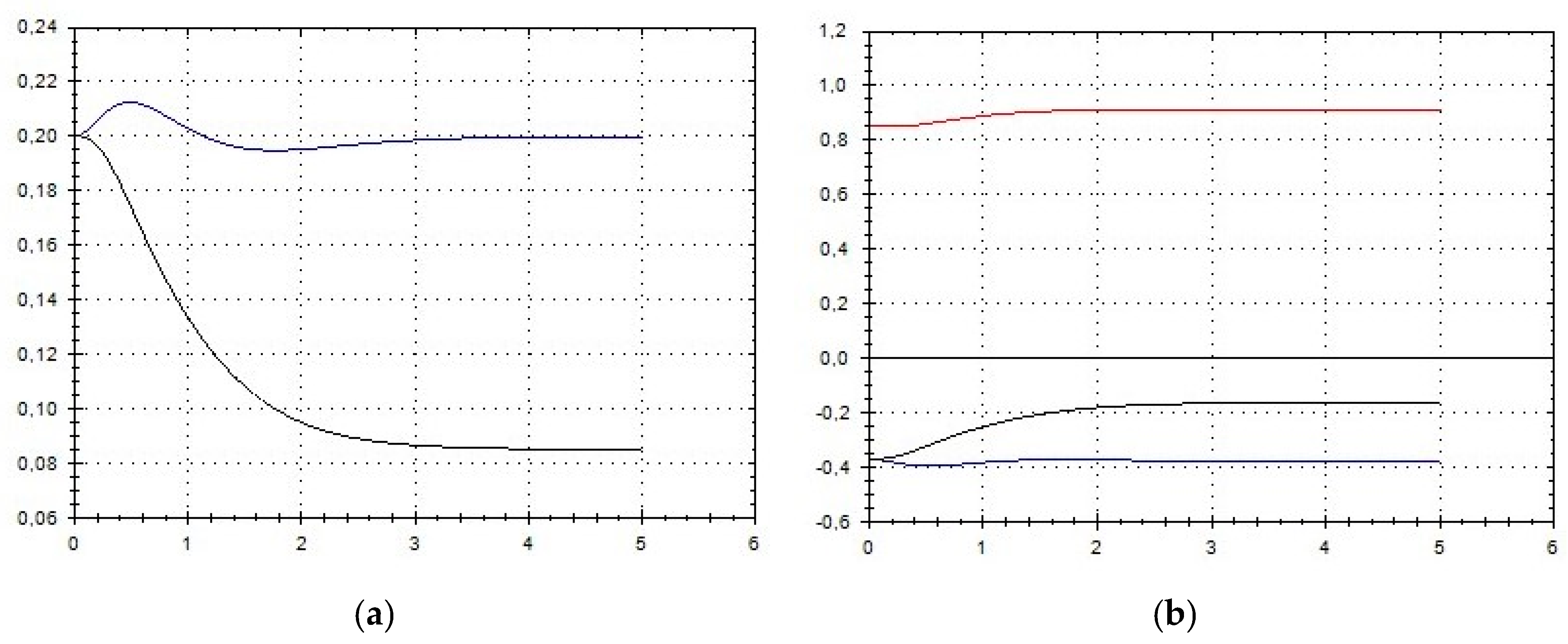
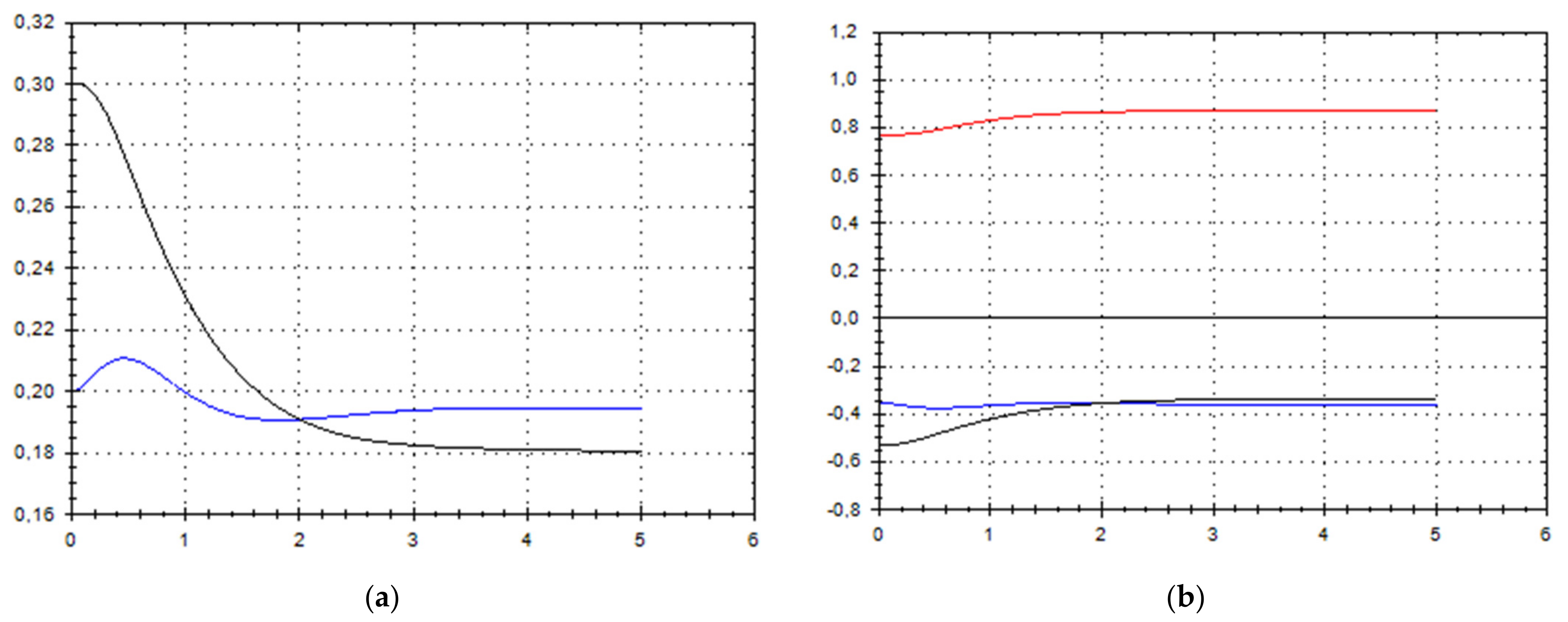
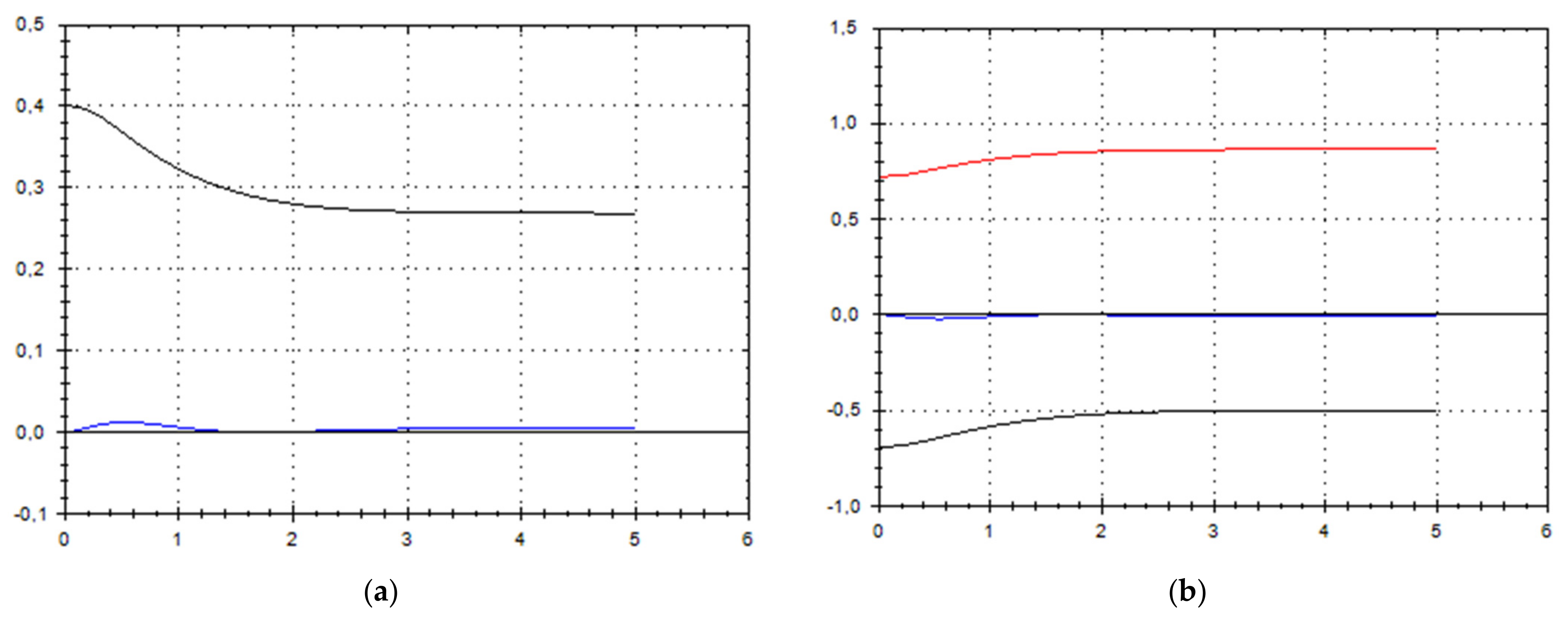
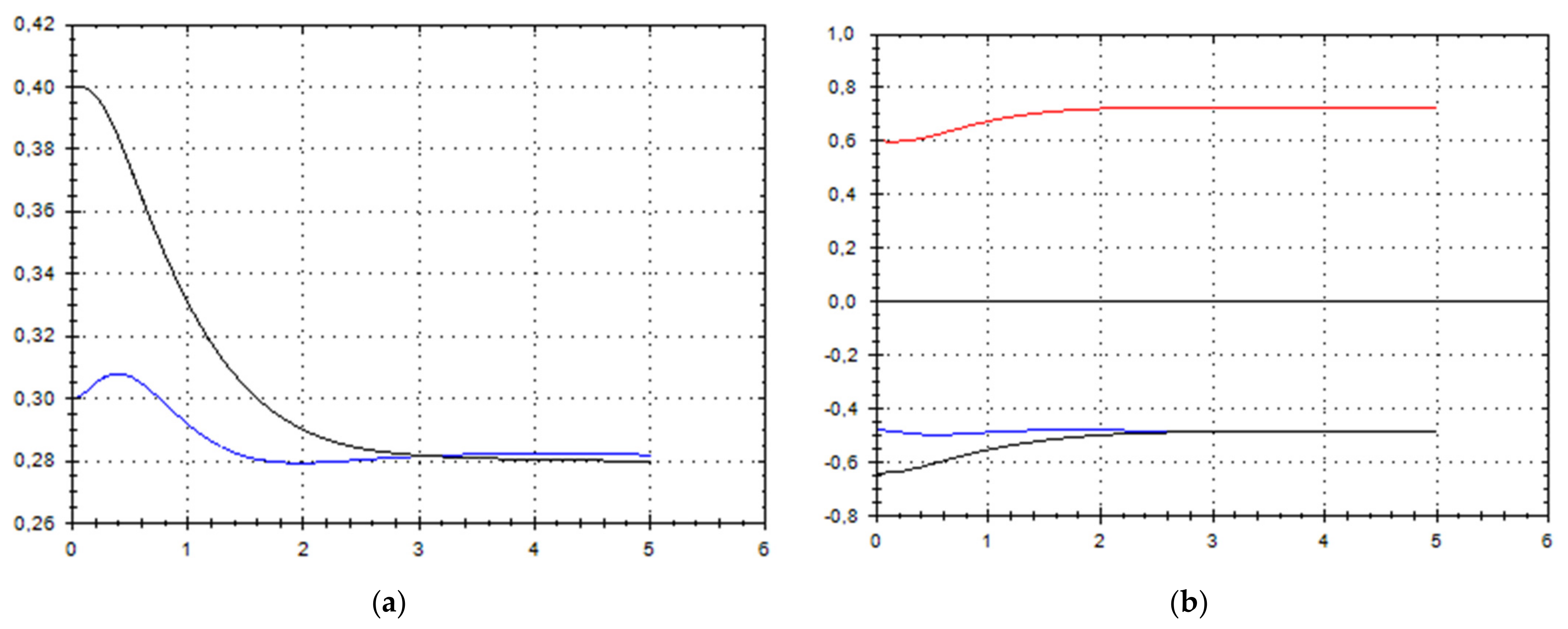
Let us schematically imagine at Figure 1, Figure 2, Figure 3, Figure 4, Figure 5, Figure 6, Figure 7, Figure 8, Figure 9, Figure 10, Figure 11 and Figure 12, the appropriate components of velocity field {u₁, u₂, u₃}, according to Formula (10) (which corresponds to the approximate solutions of system (9) for {a, b}, as well as to the chosen parameters of asymptotic flow (5) given in Figure 13), as well as let us imagine solutions {a, b} themselves there. We should note that we have used, for calculating the data, the Runge–Kutta fourth-order method with a step of 0.001 starting from initial values:

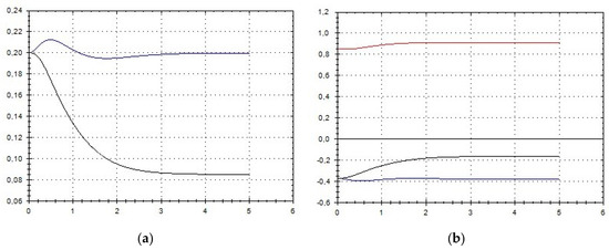
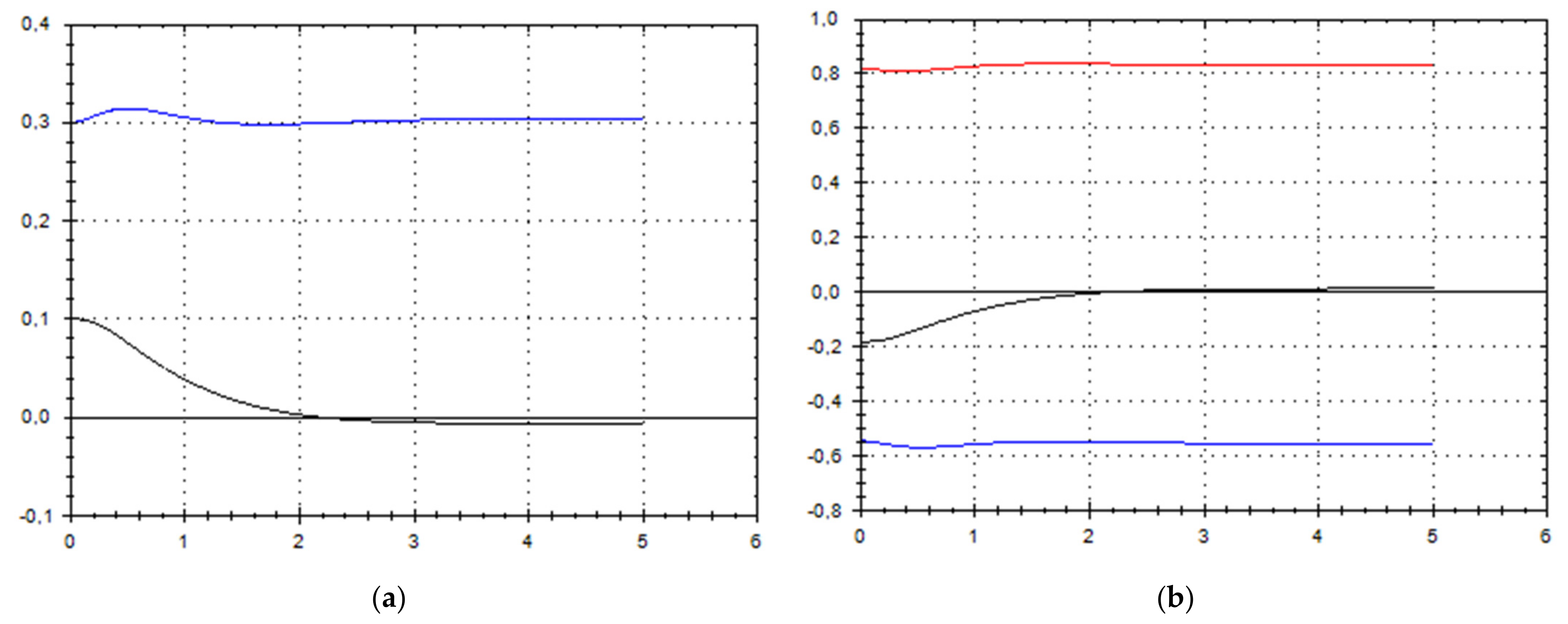
Figure 1. (a) A schematic plot of approximate solutions {a, b} of system (9), depending on time t (a is in black, b in blue). We have chosen initial data as follows: $a(0)=0.2, b(0)=0.2$. (b) A schematic plot of approximate components {u₁, u₂, u₃} of velocity field (10), depending on time t (u₁ is in black, u₂ in blue, u₃ in red). We have chosen initial data as follows: $a(0)=0.2, b(0)=0.2$, $\gamma =1.5$.

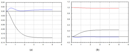
Figure 2. (a) A schematic plot of approximate solutions {a, b} of system (9), depending on time t (a is in black, b in blue). We have chosen initial data as follows: $a(0)=0\hspace{0.33em},\hspace{0.33em}\hspace{0.33em}b(0)=0$. (b) A schematic plot of approximate components {u₁, u₂, u₃} of velocity field (10), depending on time t (u₁ is in black, u₂ in blue, u₃ in red). We have chosen initial data as follows: $a(0)=0 ,\hspace{0.33em}b(0)=0$.

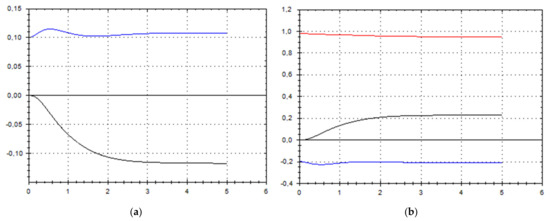
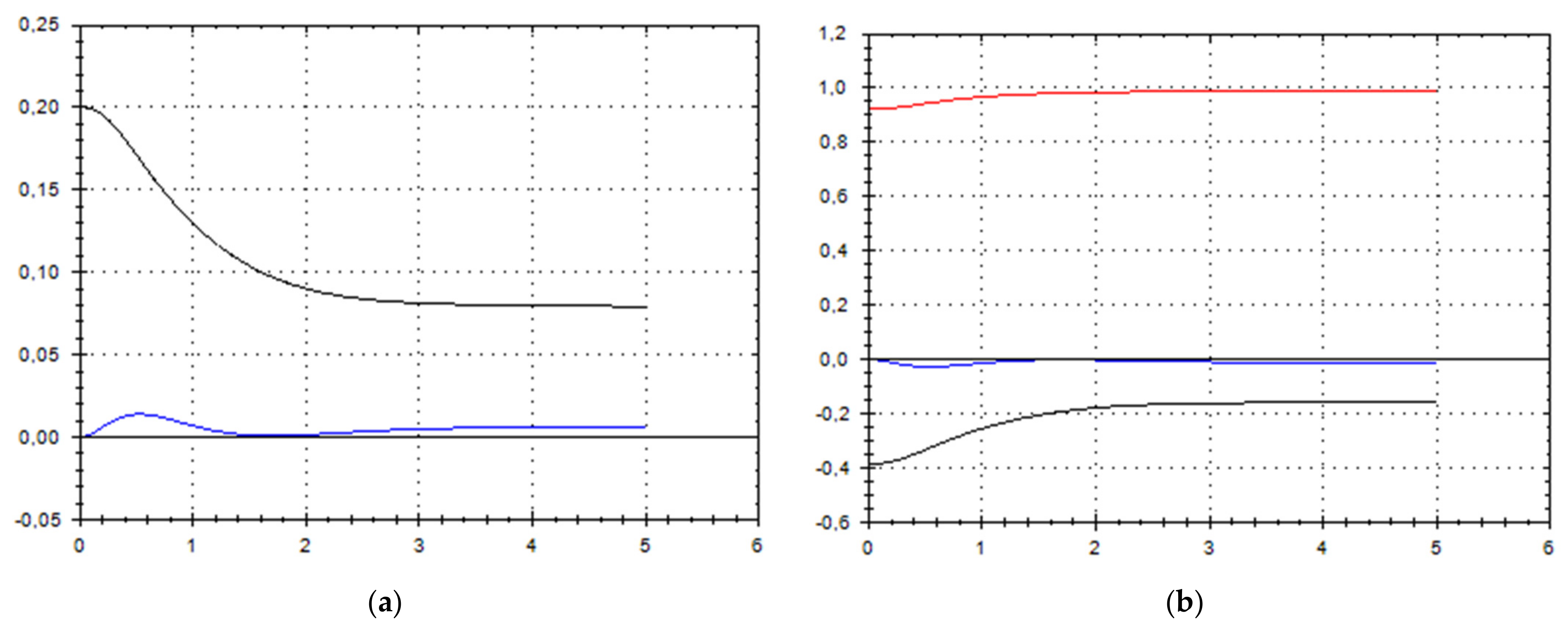
Figure 3. (a) A schematic plot of approximate solutions {a, b} of system (9), depending on time t (a is in black, b in blue). We have chosen initial data as follows: $a(0)=0\hspace{0.33em},\hspace{0.33em}\hspace{0.33em}b(0)=0.1$. (b) A schematic plot of approximate components {u₁, u₂, u₃} of velocity field (10), depending on time t (u₁ is in black, u₂ in blue, u₃ in red). We have chosen initial data as follows: $a(0)=0 ,\hspace{0.33em}b(0)=0.1$.

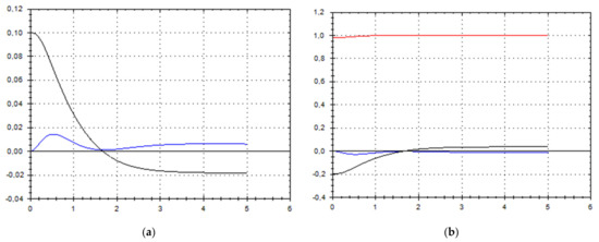
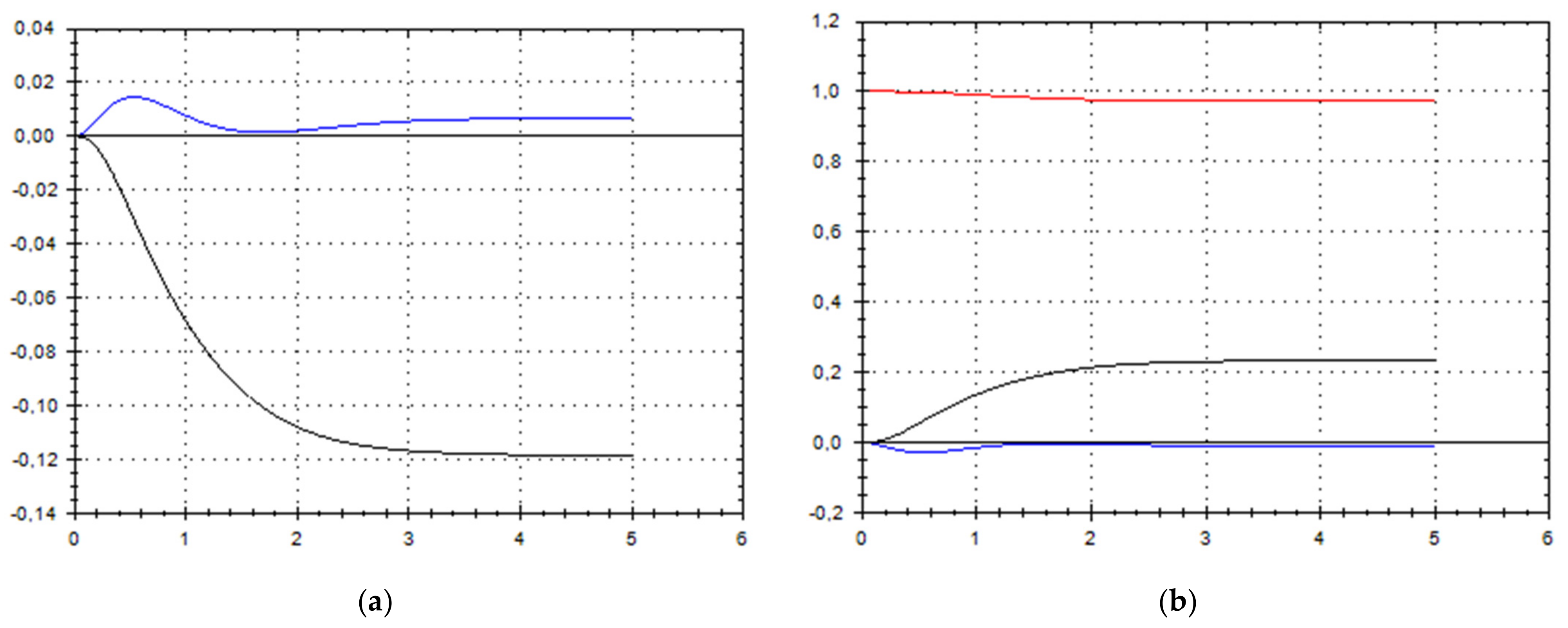
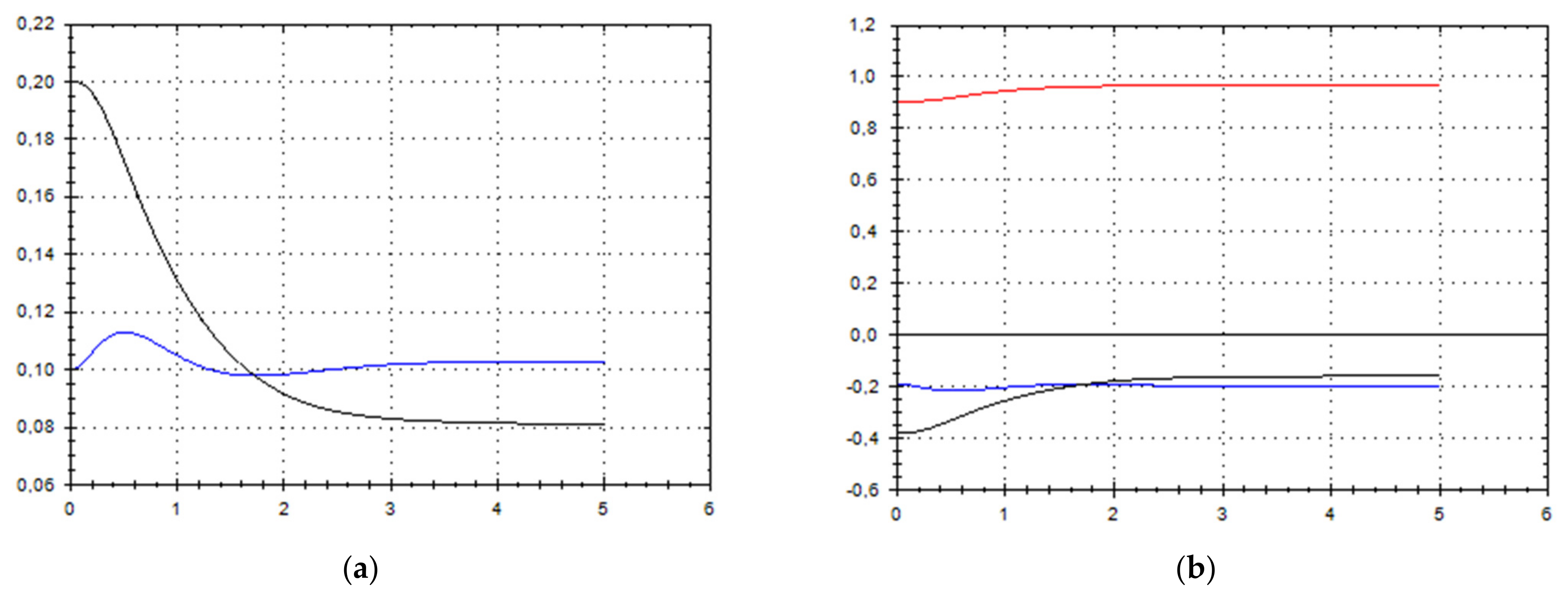
Figure 4. (a) A schematic plot of approximate solutions {a, b} of system (9), depending on time t (a is in black, b in blue). We have chosen initial data as follows: $a(0)=0.1\hspace{0.33em},\hspace{0.33em}\hspace{0.33em}b(0)=0$. (b) A schematic plot of approximate components {u₁, u₂, u₃} of velocity field (10), depending on time t (u₁ is in black, u₂ in blue, u₃ in red). We have chosen initial data as follows: $a(0)=0.1 ,\hspace{0.33em}b(0)=0$.

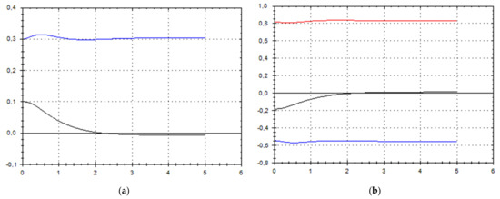
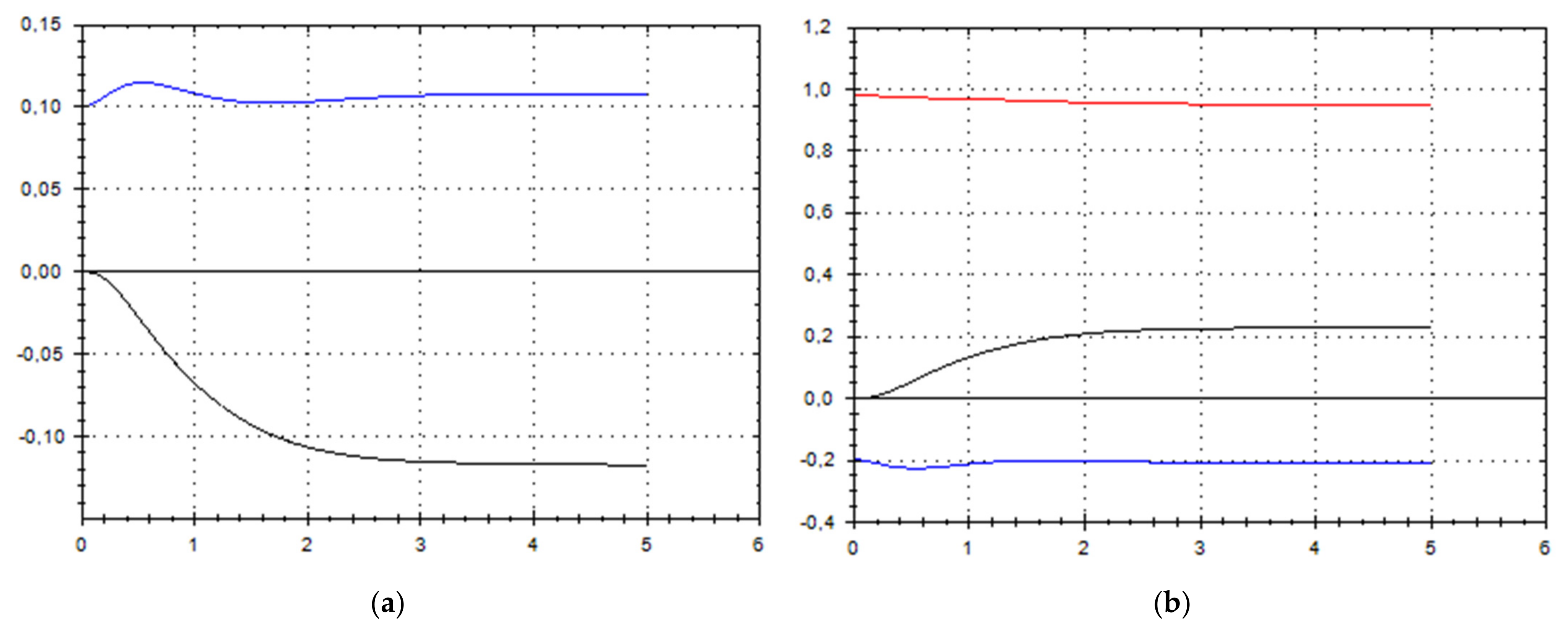
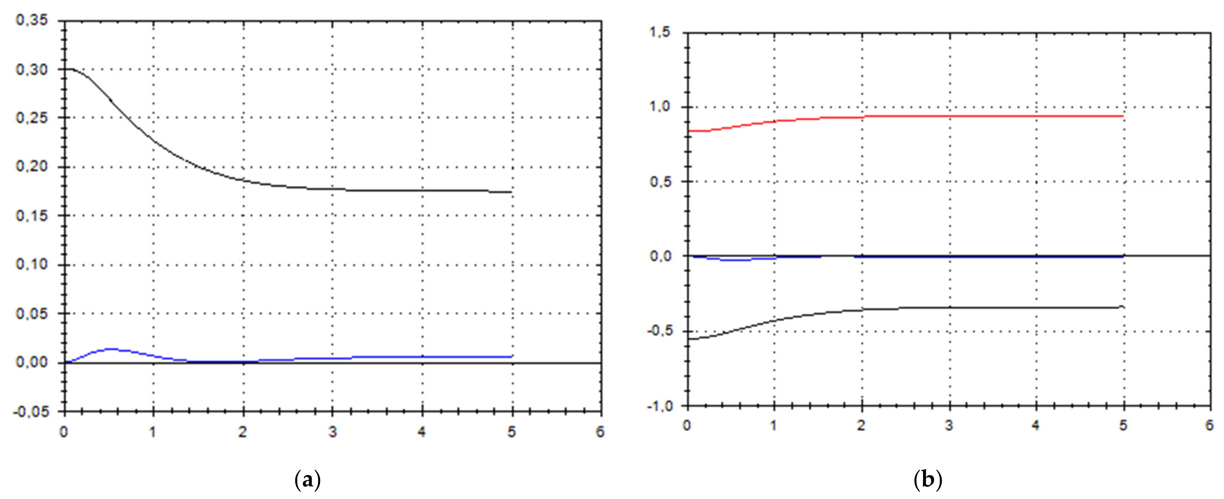
Figure 5. (a) A schematic plot of approximate solutions {a, b} of system (9), depending on time t (a is in black, b in blue). We have chosen initial data as follows: $a(0)=0.1\hspace{0.33em},\hspace{0.33em}\hspace{0.33em}b(0)=0.3$. (b) A schematic plot of approximate components {u₁, u₂, u₃} of velocity field (10), depending on time t (u₁ is in black, u₂ in blue, u₃ in red). We have chosen initial data as follows: $a(0)=0.1 ,\hspace{0.33em}b(0)=0.3$.

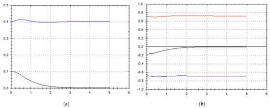
Figure 6. (a) A schematic plot of approximate solutions {a, b} of system (9), depending on time t (a is in black, b in blue). We have chosen initial data as follows: $a(0)=0.1,\hspace{0.33em}\hspace{0.33em}b(0)=0.4$. (b) A schematic plot of approximate components {u₁, u₂, u₃} of velocity field (10), depending on time t (u₁ is in black, u₂ in blue, u₃ in red). We have chosen initial data as follows: $a(0)=0 .1 ,\hspace{0.33em}b(0)=0.4$.

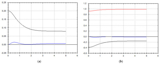
Figure 7. (a) A schematic plot of approximate solutions {a, b} of system (9), depending on time t (a is in black, b in blue). We have chosen initial data as follows: $a(0)=0.2\hspace{0.33em},\hspace{0.33em}\hspace{0.33em}b(0)=0$. (b) A schematic plot of approximate components {u₁, u₂, u₃} of velocity field (10), depending on time t (u₁ is in black, u₂ in blue, u₃ in red). We have chosen initial data as follows: $a(0)=0.2 ,\hspace{0.33em}b(0)=0$.

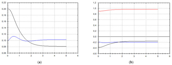
Figure 8. (a) A schematic plot of approximate solutions {a, b} of system (9), depending on time t (a is in black, b in blue). We have chosen initial data as follows: $a(0)=0.2\hspace{0.33em},\hspace{0.33em}\hspace{0.33em}b(0)=0.1$. (b) A schematic plot of approximate components {u₁, u₂, u₃} of velocity field (10), depending on time t (u₁ is in black, u₂ in blue, u₃ in red). We have chosen initial data as follows: $a(0)=0 .2 ,\hspace{0.33em}b(0)=0.1$.

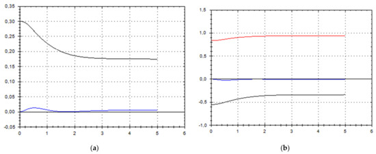
Figure 9. (a) A schematic plot of approximate solutions {a, b} of system (9), depending on time t (a is in black, b in blue). We have chosen initial data as follows: $a(0)=0.3\hspace{0.33em},\hspace{0.33em}\hspace{0.33em}b(0)=0$. (b) A schematic plot of approximate components {u₁, u₂, u₃} of velocity field (10), depending on time t (u₁ is in black, u₂ in blue, u₃ in red). We have chosen initial data as follows: $a(0)=0.3 ,\hspace{0.33em}b(0)=0$.

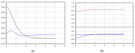
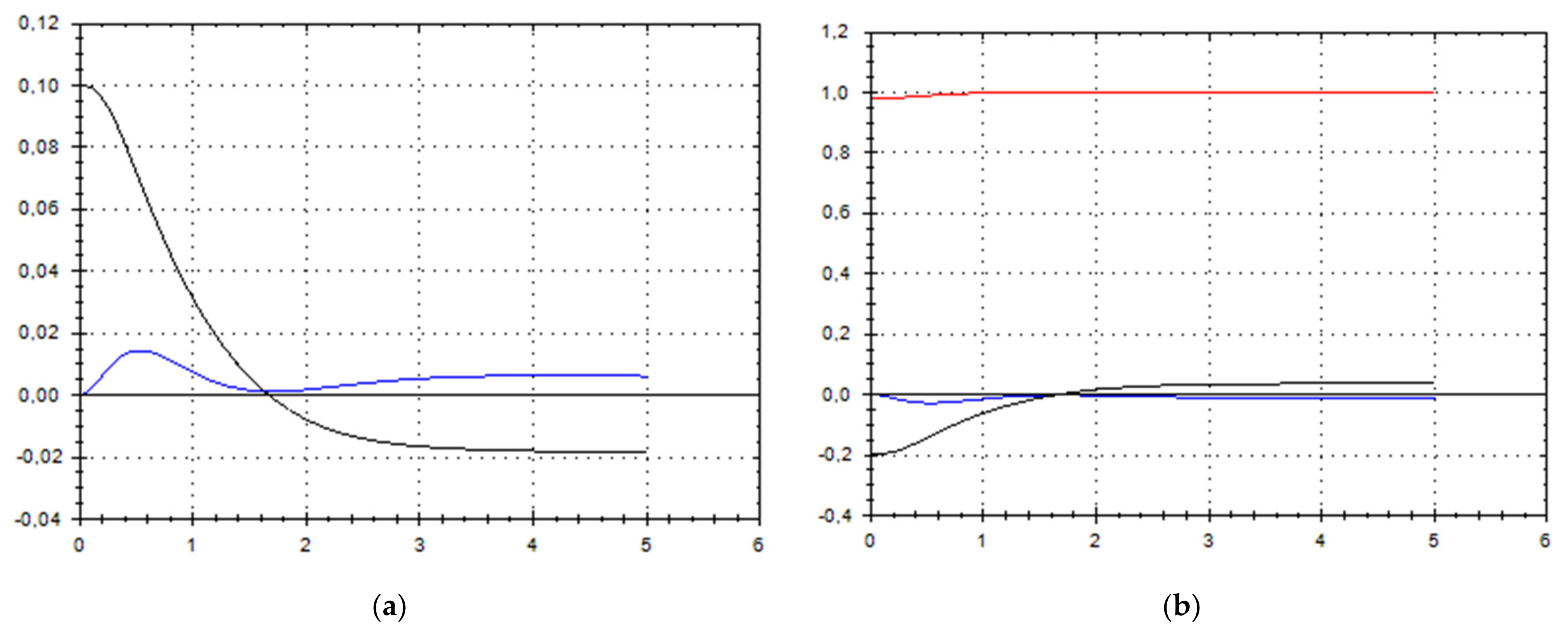
Figure 10. (a) A schematic plot of approximate solutions {a, b} of system (9), depending on time t (a is in black, b in blue). We have chosen initial data as follows: $a(0)=0.3\hspace{0.33em},\hspace{0.33em}\hspace{0.33em}b(0)=0.2$. (b) A schematic plot of approximate components {u₁, u₂, u₃} of velocity field (10), depending on time t (u₁ is in black, u₂ in blue, u₃ in red). We have chosen initial data as follows: $a(0)=0.3 ,\hspace{0.33em}b(0)=0.2$.

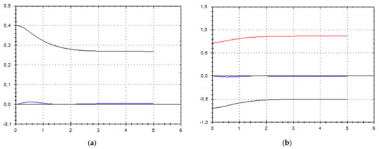
Figure 11. (a) A schematic plot of approximate solutions {a, b} of system (9), depending on time t (a is in black, b in blue). We have chosen initial data as follows: $a(0)=0.4\hspace{0.33em},\hspace{0.33em}\hspace{0.33em}b(0)=0$. (b) A schematic plot of approximate components {u₁, u₂, u₃} of velocity field (10), depending on time t (u₁ is in black, u₂ in blue, u₃ in red). We have chosen initial data as follows: $a(0)=0.4 ,\hspace{0.33em}b(0)=0$.

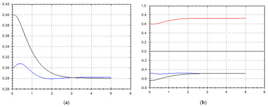
Figure 12. (a) A schematic plot of approximate solutions {a, b} of system (9), depending on time t (a is in black, b in blue). We have chosen initial data as follows: $a(0)=0.4\hspace{0.33em},\hspace{0.33em}\hspace{0.33em}b(0)=0.3$. (b) A schematic plot of approximate components {u₁, u₂, u₃} of velocity field (10), depending on time t (u₁ is in black, u₂ in blue, u₃ in red). We have chosen initial data as follows: $a(0)=0.4 ,\hspace{0.33em}b(0)=0.3$.

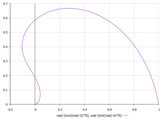
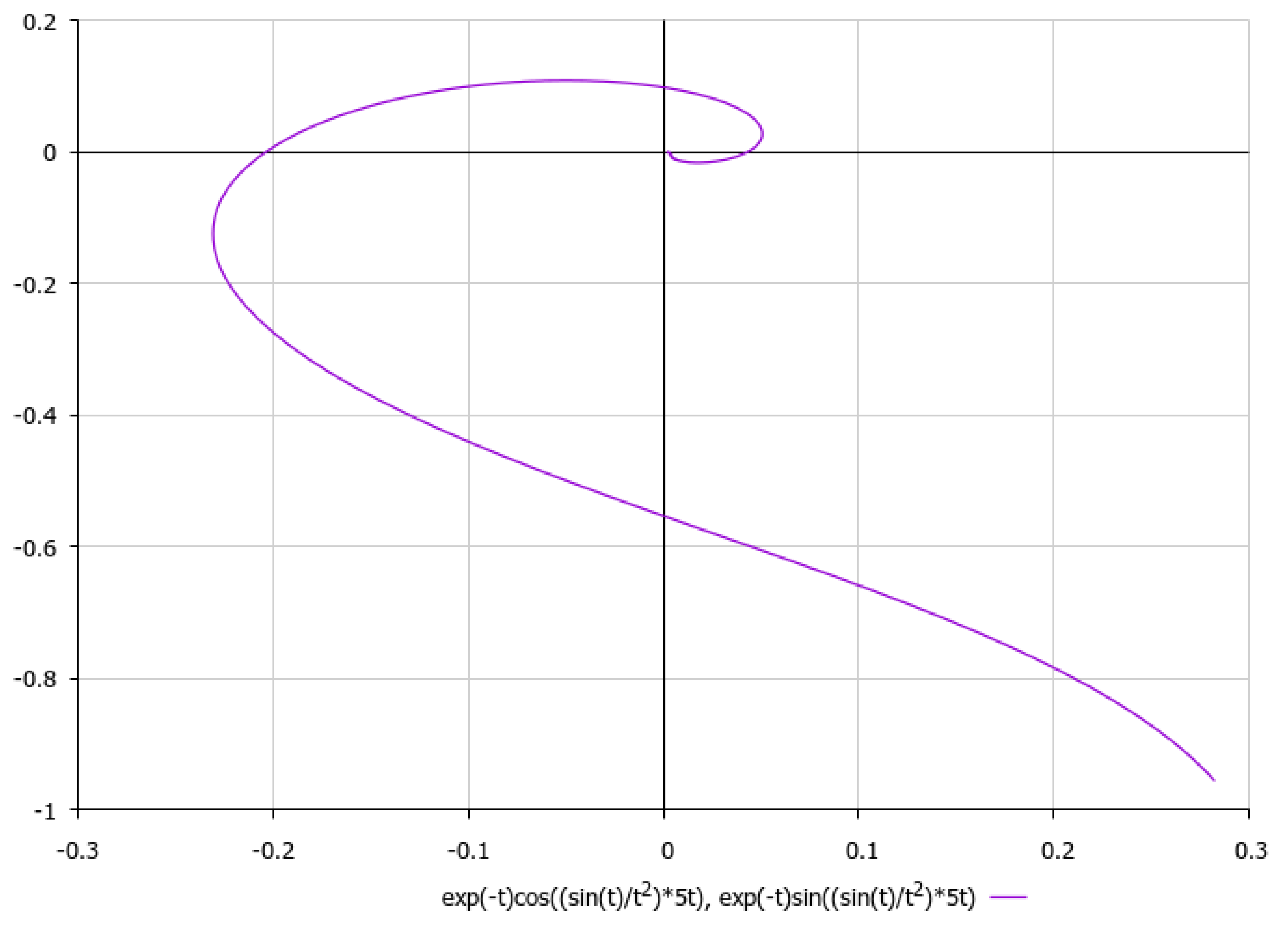
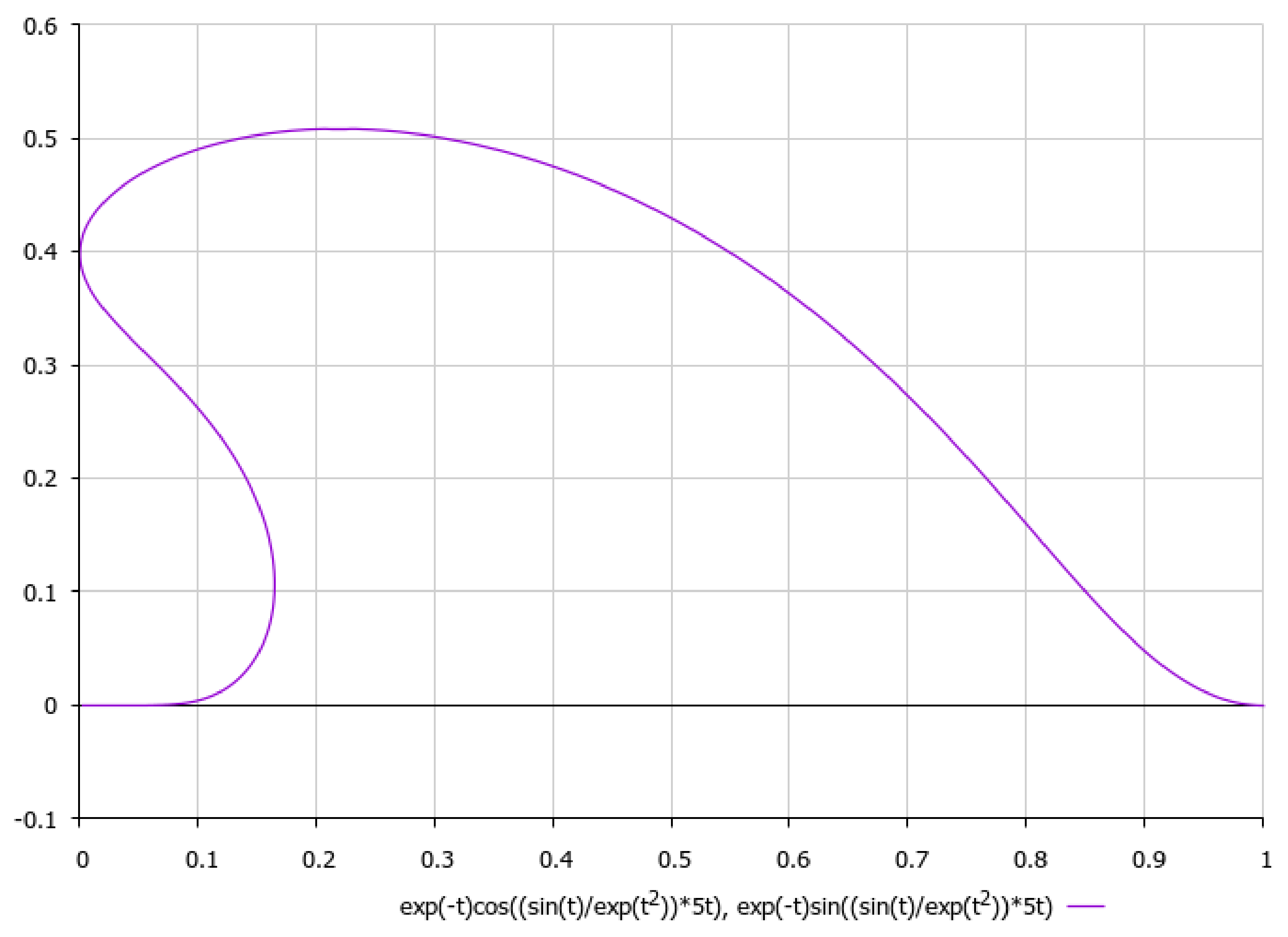
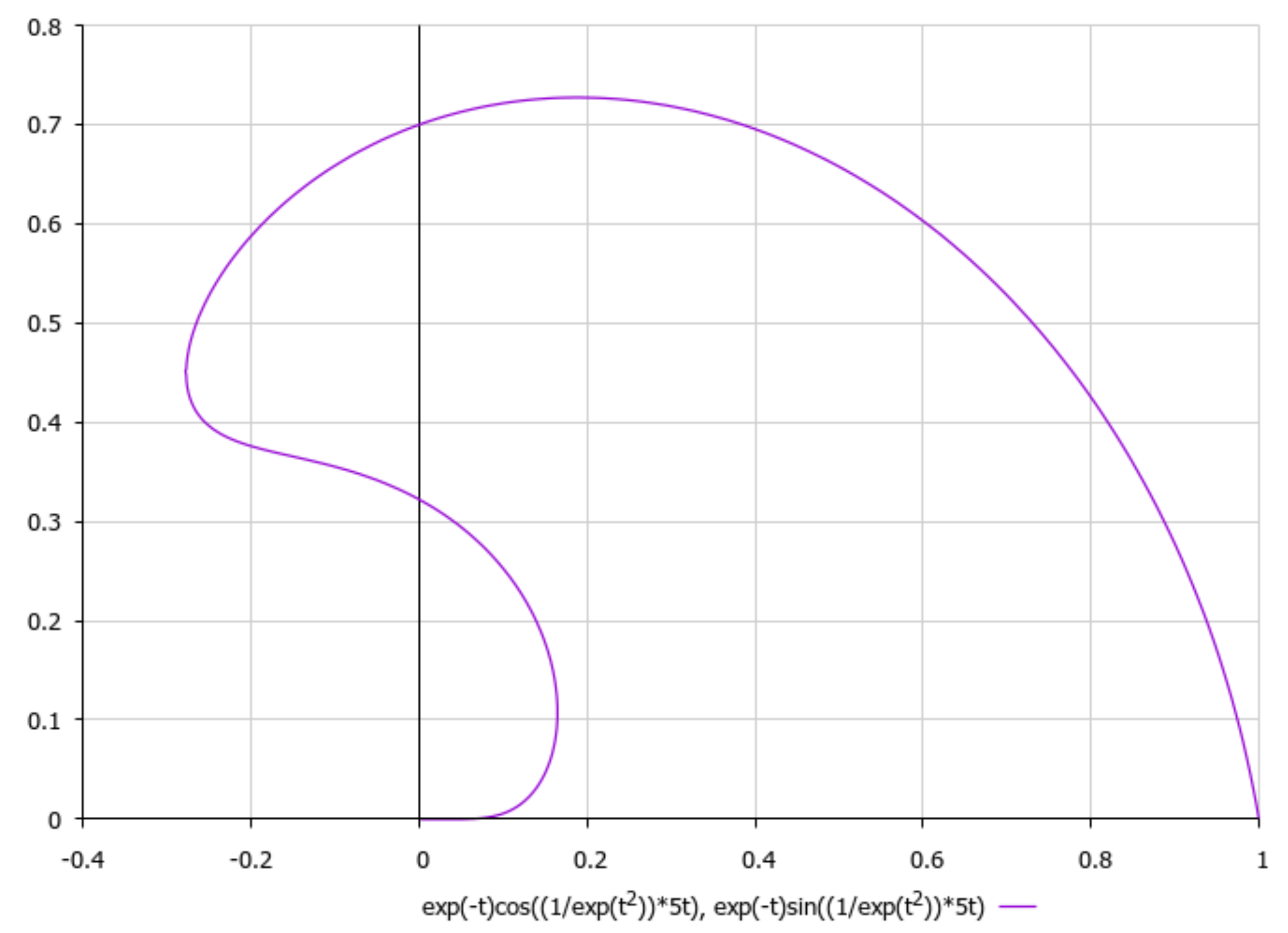
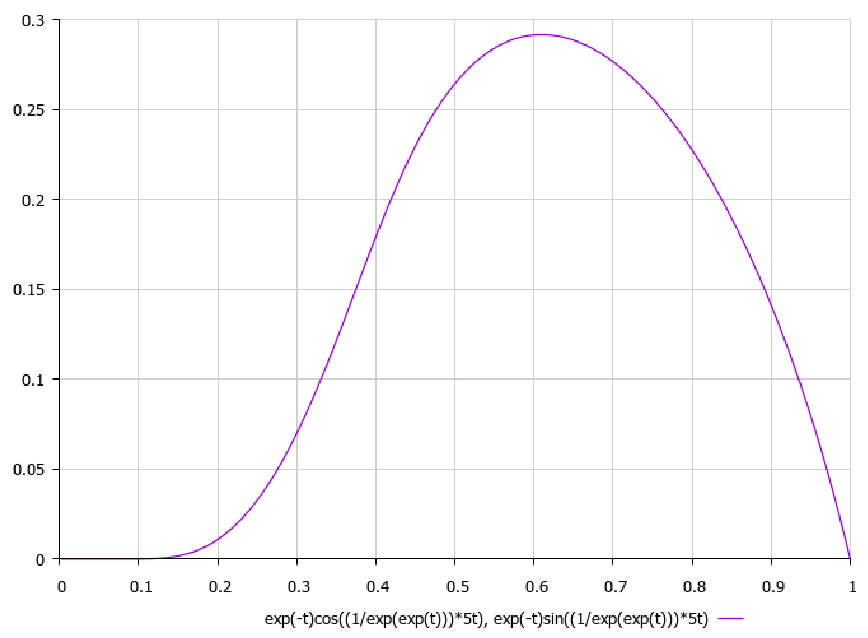
Figure 13. A schematic plot of external spiral-type flow (5), $\sigma (t)=\exp (- t) ,\hspace{0.33em}A(t)=z\exp (- t) ,\hspace{0.33em}z=5$.

Here and below, we have presented a series of numerical experiments for chosen parameters as follows $\gamma =1.5\hspace{0.33em},\hspace{0.33em}\hspace{0.33em}\frac{\partial \gamma }{\partial x}=\frac{\partial \gamma }{\partial y}=0.001$:

5. Discussion

As we can see from Figure 1, Figure 2, Figure 3, Figure 4, Figure 5, Figure 6, Figure 7, Figure 8, Figure 9, Figure 10, Figure 11 and Figure 12, we have presented here semi-analytical solutions for ideal fluid flows (governed by Euler full equations, Equations (1) and (2)), driven by external large-scale coherent structure of spiral-type presented in Figure 13. Most of them (except for Figure 5, Figure 6 and Figure 12) are presented by dynamically upwelling 3D non-stationary flows with significant 3rd component of motion, with respect to 1st and 2nd components of fluid flow. The intriguing fact is that, in Figure 4b and Figure 5b, we can see the examples of reverse flows where amplitude of the first component of solution is changing its sign to the opposite.

It is worth noting, with respect to presenting the asymptotics of non-stationary three-dimensional solutions of external non-viscous rotational flow (5), that we should obtain under aforementioned simplifying assumption γ² >> σ², that if we choose, e.g., $\sigma = \alpha \exp (\pm \beta t)$, it would yield a 2D logarithmic spiral (here {α,β} are positive constants) for which third component of velocity field $W(x,y,t) = \sqrt{{\gamma }^2 (x,y)-{\sigma }^2(t)}\cong \gamma (x,y)$ could be considered as to be approximately constant with respect to the time-parameter t. Let us schematically imagine at Figure 13, Figure 14, Figure 15, Figure 16 and Figure 17, the appropriate graphical plots of velocity field (5) (asymptotics of external rotational flow, z = 5), which demonstrate extremely nonlinear dynamics.

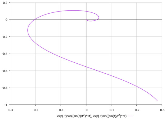
Figure 14. A schematic plot of external spiral-type flow (5), $\sigma (t)=\exp (- t) ,\hspace{0.33em}\hspace{0.33em}A(t)=z\sin ( t)/t^{ 2}$.

Figure 15. Schematic plot of external spiral-type flow (5), $\sigma (t)=\exp (- t) ,\hspace{0.33em}A(t)=z\sin ( t)/\exp (t^{ 2})$.

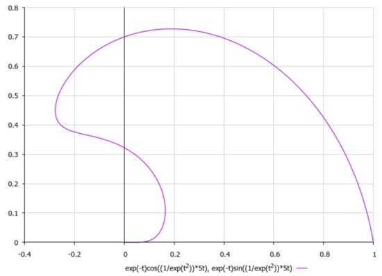
Figure 16. A schematic plot of external spiral-type flow (5), $\sigma (t)=\exp (- t) ,\hspace{0.33em}\hspace{0.33em}A(t)=z/\exp (t^{ 2})$.

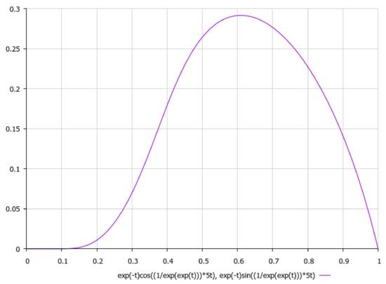
Figure 17. A schematic plot of external spiral-type flow (5), $\sigma (t)=\exp (- t) ,\hspace{0.33em}A(t)=z/\exp (\exp (t))$.

We can see that the most realistic cases have been presented in Figure 13, Figure 14, Figure 15, Figure 16 and Figure 17, with respect to the appropriate graphical plots of velocity field (5), namely the asymptotics of external rotational flows (for z = 5), which could be forming the coastline geometry of a bay or topology of the bottom surface in various parts of the ocean.

The last but not least, we should especially note that we have presented here the appropriate solving procedure for modelling the semi-analytical solutions for ideal fluid flows driven by external large-scale coherent structures of spiral-type, but in cases for which we do not choose to consider any of the restrictions $\left\{\begin{array}{c}\\ \end{array}\right.\sigma (t) ,\hspace{0.33em}A(z,t) ,\hspace{0.33em}\left(\frac{\partial A(z,t)}{\partial z}\right)\left.\begin{array}{c}\\ \end{array}\right\} \ne 0$ we should definitely obtain in result, the variations of analytical solution of periodic-type, which was firstly presented in [11] (with linear dependence of function a(t) on function b(t) in (9), whereas a(t) is linearly dependent on tan(f(t)) where f(t) is linear function of time or even nonlinear function of time in special cases of proportionality between coefficients in the aforementioned restrictions to each other).

In addition, some remarkable articles should be cited, which concern the problem under consideration [12,13,14,15,16,17,18]. In [12], the formation and shedding of vortices in two vortex-dominated flows around an actuated flat plate are studied to develop a better method of identifying and tracking coherent structures in unsteady flows. In [13], authors model the ionospheric–thermospheric flows with the Thermosphere-Ionosphere-Electrodynamics General Circulation Model and identify the Lagrangian coherent structures, which are objective ridges in time-evolving flows that describe the tendency of neighboring fluid elements to separate, providing a unique opportunity to infer the dynamics in the ionospheric–thermospheric system. In [14], it was reported the interaction between active non-spherical swimmers and a long-standing flow structure (Lagrangian coherent structures), in a weakly turbulent two-dimensional flow by using a hybrid experimental–numerical model. In [15], the unsteady phenomena of vertical-axis turbine wake-flow were analyzed in two rotational speed conditions from a Lagrangian perspective. In the sound research [16], the proper formation of a canonical vortex ring is performed to investigate the nature of vortex added-mass and explore a solution for estimating the vortex added-mass coefficient (where the ridges of finite-time Lyapunov exponent are applied to identify the Lagrangian boundary of the vortex ring). In [17], the three-dimensional transport pathways, the time and space scales of vertical transport, and the dispersion characteristics of submesoscale currents at an upper-ocean front, are investigated using tracing particles. Let us outline that the authors of [17] found a number of coherent vortex filaments and eddies, generated and sustained during the evolution of baroclinic instability (including one’s which are forming structures through coherent, anisotropic submesoscale motions). In a very useful (from practical point of view) investigation [18], authors explored the Lagrangian coherent structure of Laizhou Bay which was calculated based on the appropriate hydrodynamic simulation by them. The results have shown, in particular (but not limited to), that the theory of Lagrangian coherent structure is a powerful tool to explain the complex flow phenomena and has reference significance for studying offshore material transport.

6. Conclusions

We have presented here the clearly formulated algorithm or semi-analytical solving procedure for obtaining (or tracing) the approximate hydrodynamical fields of flows (and thus, their trajectories) for ideal incompressible fluids governed externally by large-scale coherent structures of spiral-type (e.g., which are based on “wind-water-coastline” interactions during a long-time period), which can be recognized as special invariant at symmetry reduction.

Indeed, we have started our research from introducing the partial form of coherent structures of spiral-type (5), which may play a role of external driving process for ideal fluid flows governed by Euler equations (Equations (1), (2), or (3)) (via mechanism of rotation which corresponds to the actual giving of the curl field in incompressible fluids).

Then, we have suggested to investigate (as first approximation) such solutions of Euler equations (Equations (1), (2), or (3)) which should conserve the Bernoulli-function (4) for the flow in the whole space (considering the Cauchy problem in the whole space).

We should especially note that results of the current research can be generalized to the case of non-stationary Bernoulli-function (e.g., to the case of changing the variables {x,y,z} considered in Equations (6)–(10) as parameters, or even to the time-dependent case, or moreover to the most complex case of their combination) for the reason that system of Equation (3) with $\nabla B\hspace{0.33em}\ne \hspace{0.33em}0$ could be theoretically considered as having been solved, as reported in [11], if we obtain a general solution for the corresponding homogeneous system (3) (i.e., in case $\nabla B\hspace{0.33em}=\hspace{0.33em}0$).

It is also worth noting that solutions of system (9) can be easily generalized up to a 3D case if we do not take into account the simplifying assumption $\left(\frac{\partial A(z,t)}{\partial z}\right) = \mathsf{\Omega }(t)$ for solutions (8). However, nevertheless, in this case, the resulting system of ODE will look very complicated with respect to the one presented by Equation (9), as well as such system in any case will require additional simplifications for its successful numerical solving procedure.

The aforementioned approach quite differs from that which was used previously in investigation of Euler equations in [6] by two of the authors. Indeed, the approach suggested in the current research assumes the approximated solution (with numerical findings) which stems from Equation (7) with approximated components of a vortex field (8) in the fluid, whereas in [6] a kind of exact solution has been basically proposed with further semi-analytical ansatz for the solving procedure to obtain particular solutions along with their graphical plots.

The relevant restrictions at choosing of the form of 3D solution for the given constant Bernoulli-function B are emphasized: for example, the pressure field should be calculated from the given constant Bernoulli-function B, if all the components of velocity field are obtained. In addition, restrictions for choosing function ξ(x,y,z) for the aforementioned solutions stem from the continuity equation (Equation (1)).

References

- Samelson, R.M. Lagrangian Motion, Coherent Structures, and Lines of Persistent Material Strain. Annu. Rev. Mar. Sci. 2013, 5, 137–163. [Google Scholar] [CrossRef] [PubMed] [Green Version]
- Malhotra, N.; Mezić, I.; Wiggins, S. Patchiness: A new diagnostic for Lagrangian trajectory analysis in time-dependent fluid flows. Int. J. Bifurc. Chaos 1998, 8, 1053–1093. [Google Scholar] [CrossRef]
- Gnosh, A.; Suara, K.; Yu, Y.; Zhang, H.; Brown, R.J. Using Lagrangian Coherent Structures to Investigate Tidal Transport Barriers in Moreton Bay, Queensland. In Proceedings of the 21st Australasian Fluid Mechanics Conference Adelaide, Adelaide, Australia, 10–13 December 2018. [Google Scholar]
- Saffman, P.G. Vortex Dynamics; Cambridge University Press: Cambridge, UK, 1995. [Google Scholar]
- Landau, L.D.; Lifshitz, E.M. Fluid Mechanics, Course of Theoretical Physics 6, 2nd ed.; Pergamon Press: Cambridge, UK, 1987; ISBN 0-08-033932-8. [Google Scholar]
- Ershkov, S.V.; Shamin, R.V. A Riccati-type solution of 3D Euler equations for incompressible flow. J. King Saud Univ.-Sci. 2020, 32, 125–130. [Google Scholar] [CrossRef]
- Ershkov, S.V. On Existence of General Solution of the Navier-Stokes Equations for 3D Non-Stationary Incompressible Flow. Int. J. Fluid Mech. Res. 2015, 42, 206–213. [Google Scholar] [CrossRef] [Green Version]
- Ershkov, S.V. Non-stationary Riccati-type flows for incompressible 3D Navier-Stokes equations. Comput. Math. Appl. 2015, 71, 1392–1404. [Google Scholar] [CrossRef]
- Ershkov, S.V. A procedure for the construction of non-stationary Riccati-type flows for incompressible 3D Navier-Stokes equations. Rend. Circ. Mat. Palermo 2016, 65, 73–85. [Google Scholar] [CrossRef] [Green Version]
- Ershkov, S.V.; Giniyatullin, A.R.; Shamin, R.V. On a new type of non-stationary helical flows for incompressible 3D Navier-Stokes equations. J. King Saud Univ.-Sci. 2020, 32, 459–467. [Google Scholar] [CrossRef]
- Ershkov, S.V.; Shamin, R.V. On a new type of solving procedure for Laplace tidal equation. Phys. Fluids 2018, 30, 127107. [Google Scholar] [CrossRef] [Green Version]
- Huang, Y.; Green, M.A. Detection and tracking of vortex phenomena using Lagrangian coherent structures. Exp. Fluids 2015, 56, 147. [Google Scholar] [CrossRef]
- Wang, N.; Dand, T.; Lei, I.; Wang, W.; Datta-Barrua, S. Alignment of High-Latitude Ionospheric and Thermospheric Lagrangian Coherent Structures. J. Geophys. Res.: Space Phys. 2021, 126, e2020JA029028. [Google Scholar] [CrossRef]
- Si, X.; Fang, L. Preferential alignment and heterogeneous distribution of active non-spherical swimmers near Lagrangian coherent structures. Phys. Fluids 2021, 33, 073303. [Google Scholar] [CrossRef]
- Wang, K.; Zou, L.; Zhang, I.; Jiang, Y.; Zhao, P. Lagrangian coherent structures and material transport in unsteady flow of vertical-axis turbine wakes. AIP Adv. 2021, 11, 085001. [Google Scholar] [CrossRef]
- Lin, S.-J.; Xiang, Y.; Li, Z.-Q.; Wang, F.-X.; Liu, H. Evolution of the Lagrangian drift and vortex added-mass of a growing vortex ring. J. Hydrodyn. 2021, 33, 725–735. [Google Scholar] [CrossRef]
- Verma, V.; Sarkar, S. Lagrangian three-dimensional transport and dispersion by submesoscale currents at an upper-ocean front. Ocean Model. 2021, 165, 101844. [Google Scholar] [CrossRef]
- Zhang, Y.-W.; Feng, Y.-L.; Feng, C.-A.; Wang, Z.-W.; Zhang, X.-Q. Study on Lagrangian Coherent Structure of tidal current field in Laizhou Bay. Shuidonglixue Yanjiu yu Jinzhan/Chin. J. Hydrodyn. Ser. A 2021, 36, 95–101. [Google Scholar]
- Koptev, A.V. Generator of solutions for 2D Navier-Stokes equations. J. Sib. Fed. Univ. 2014, 7, 324–330. [Google Scholar]
- Koptev, A.V. Integrals of Motion of an Incompressible Medium Flow. From Classic to Modern. In Handbook of Navier-Stokes Equations: Theory and Applied Analysis; Nova Science Publishers: New York, NY, USA, 2017; pp. 443–460. [Google Scholar]
- Koptev, A.V. Method for Solving the Navier-Stokes and Euler Equations of Motion for Incompressible Media. J. Math. Sci. 2020, 250, 10–21. [Google Scholar] [CrossRef]
- Koptev, A.V. Exact Solutions of 3D Navier-Stokes Equations. J. Sib. Fed. Univ. Math. Phys. 2020, 13, 306–313. [Google Scholar] [CrossRef]
- Semenov, V.I. Some new identities for solenoidal fields and applications. Mathematics 2014, 2, 29–36. [Google Scholar] [CrossRef] [Green Version]
Publisher’s Note: MDPI stays neutral with regard to jurisdictional claims in published maps and institutional affiliations. |
© 2021 by the authors. Licensee MDPI, Basel, Switzerland. This article is an open access article distributed under the terms and conditions of the Creative Commons Attribution (CC BY) license (https://creativecommons.org/licenses/by/4.0/).