Applicable Image Security Based on New Hyperchaotic System

Abstract

Hyperchaotic systems are widely applied in the cryptography domain on account of their more complex dynamical behavior. In view of this, the greatest contribution of this paper is that a two-dimensional Sine coupling Logistic modulated Sine (2D-SCLMS) system is proposed based on Logistic map and Sine map. By a series of analyses, including Lyapunov index (LE), 0–1 test, two complexity analysis methods, and two entropy analysis methods, it is concluded that the new 2D-SCLMS map is hyperchaotic with a wider range of chaos and more complex randomness. The new system combined with two-dimensional Logistic-Sine Coupling Mapping (2D-LSCM) is further applied to an image encryption application. SHA-384 is used to generate the initial values and parameters of the two chaotic systems. Symmetric keys are generated during this operation, which can be applied to the proposed image encryption and decryption algorithms. The encryption process and the decryption process of the new image encryption approaches mainly include pixel scrambling, exclusive NOR (Xnor), and diffusion operations. Multiple experiments illustrate that this scheme has higher security and lower time complexity.

1. Introduction

Cryptography is a traditional and effective way to protect information security for a long time. According to whether the same key is used in the encryption and decryption processes, encryption can be divided into symmetric encryption and asymmetric encryption. Running symmetric encryption and decryption is relatively faster than the asymmetric encryption and decryption which usually takes a longer time. With the approach of 5G era, the amount of image data in wired and wireless communication nets is in the tens of thousands. Therefore, an efficient symmetric image encryption scheme becomes extremely important for protecting image security during storage and transmission.

Through the years, scholars have proposed multifarious image encryption schemes, such as a series of popularly known confusion and diffusion-based methods [1,2]. The framework structure of confusion and diffusion for image encryption was put forwarded by Fridrich in 1998 [3]. Confusion is usually achieved by permuting pixel control by keys without changing pixel values. Nevertheless, diffusion guarantees that altering one original pixel will cause several encrypted pixels to change.

Multifarious chaotic systems have been extensively applied to diverse fields [4,5,6,7,8,9,10,11] over the years because of their excellent properties [12,13,14,15]. Many scholars have designed robust and complex image encryption algorithms by using chaotic systems and the excellent characteristics of chaos [16,17,18,19,20,21,22,23,24,25]. When changing the initial parameters of the chaotic map, we can obtain totally different chaotic sequences. However, the premise for applying a chaotic map to image encryption is that it should have a large parameter space. Unfortunately, some classical maps, like Tent and Logistic maps, are chaotic only within a small scope of parameters. Therefore, it is essential to improve them to generate chaotic maps with more complex properties [26]. Hua et al. [27] proposed 2D-SLMM combined with CMT for image encryption. Zhu et al. [28] designed LSMCL map and combined with the substitution and diffusion methods for image encryption. Although the dimensionalities of these proposed chaotic systems are higher than those of the classical maps, their chaotic trajectories still do not spread over the whole space and their parameter space is not very large. Therefore, a new 2D system with larger parameter space and excellent chaotic properties is put forward.

To strengthen the safety of the chaotic systems and the formation of confusion- and diffusion-based image encryption, we put forward a new Sine-coupling-Logistic-modulated-Sine system based on two one-dimensional maps, which expands the results from one-dimensional to two-dimensional. To verify the better performance of the newly designed 2D-SCLMS map compared to many existing chaotic maps, the dynamics of the newly designed 2D-SCLMS map is analyzed from multiple perspectives, including chaotic trajectory, bifurcation diagram, Lyapunov exponent, two complexity analysis methods [29,30], 0–1 test [31,32], sample entropy, and permutation entropy [33]. Experimental tests show that 2D-SCLMS is a hyperchaotic system and has a wider chaotic range and better randomness.

Besides, a new symmetric encryption scheme using two new chaotic systems, which includes 2D-SCLMS map and 2D-LSCM [34], is further introduced. The procedure of the encryption scheme is realized by pixel scrambling, Xnor, and diffusion. When scrambling, we propose to scramble the image by combining the indices of two chaotic sequences generated by the 2D-SCLMS system. Diffusion consists of two parts, row diffusion and column diffusion. We make use of two other chaotic sequences to perform the row and column diffusion respectively. In addition, the SHA-384 hash is used to produce the initial parameters of two systems, which greatly improves the resistance to known plaintext and chosen plaintext attacks [33,35].

The major contributions of this paper are as follows: (1) A new two-dimensional hyperchaotic map is designed based on Logistic and Sine maps. (2) Various methods, such as chaotic trajectory, Lyapunov exponent, 0–1 test, complexity analysis methods, and two different entropy analysis methods, are used to evaluate the chaotic properties of the new two-dimensional hyperchaotic map. (3) According to the two chaotic maps, a new symmetric encryption scheme for improving image security is proposed.

The rest of this article is arranged as follows. Section 2 states related works. Section 3 proposes the new 2D-SCLMS map and analyzes its chaotic behaviors. Section 4 presents the design of the new pixel scrambling method. Section 5 demonstrates the new symmetric image encryption algorithm. Section 6 describes the corresponding image decryption process. Section 7 presents simulation experiments and safety performance analysis. Section 8 shows color image encryption. Section 9 introduces the application areas of encryption algorithms. Section 10 provides the conclusion.

2. Related Works

This section first introduces two proposed chaotic maps, which constitute the basis for creating the 2D-SCLMS map. Then, another chaotic system 2D-LSCM for image encryption algorithm is described.

2.1. Logistic Map

Pierre François Verhulst denominated this map as the Logistic map [36]. It is known for its complex dynamic properties and has been widely used in different domains. In general, the expression of a 1D Logistic map [37] is

x_i+1 = 4μ(x_i − x_i²)

(1)

where μ ∈ (0, 1) is the parameter. x_i ∈ (0, 1), i = 1, 2,⋯.

2.2. Sine Map

A variation of the sine function is Sine map whose input is converted from [0, π] to [0, 1] and whose output range [0, 1] remains unchanged. The expression of the Sine map is described as [38]:

x_i+1 = λsin(πx_i)

(2)

where λ ∈ (0, 1) is a parameter. x_i ∈ (0, 1), i = 1, 2,⋯.

2.3. 2D-LSCM

In this paper, 2D-LSCM is used as one of the chaotic systems of the encryption algorithm. The expression of the 2D-LSCM [34] is

$$\left\{\begin{array}{c}{z}_{i+1}=\sin (\pi (4\alpha (z_i-z_i^2)+(1-\alpha )\sin (\pi w_i)))\hfill \\ w_{i+1}=\sin (\pi (4\alpha (w_i-w_i^2)+(1-\alpha )\sin (\pi z_{i+1})))\hfill \end{array}\right.$$

(3)

where α ∈ [0, 1] is a parameter.

3. 2D-SCLMS Map

We propose a novel Sine-coupling-Logistic-modulated-Sine map, in view of Logistic and Sine maps. To verify the better chaotic performance of the newly 2D-SCLMS map, efficient analysis and comparison are implemented in this section.

3.1. The Newly 2D-SCLMS Map

In fact, Logistic and Sine maps have good chaotic performances only in a suitable range of parameters and they also have some drawbacks, such as simple chaos and small chaotic range. Hence, it is relatively easy to forecast their trajectories using chaotic signal estimation techniques [39,40]. To overcome these drawbacks, a new 2D-SCLMS chaotic map with better chaotic properties is constructed in this paper. It is defined by Equation (4).

$$\left\{\begin{array}{l}{x}_{i+1}=\sin (4{\pi }^2(u\sin (4\pi (x_i-x_i^2)))+4u(y_i-y_i^2))\\ y_{i+1}=\sin (4{\pi }^2(u\sin (4\pi (y_i-y_i^2)))+4u(x_{i+1}-x_{i+1}^2))\end{array}\right.$$

(4)

where u > 0.1 is the parameter. x_i, y_i ∈ (−1,1), i = 1, 2,⋯.

3.2. Performance Analysis

The 2D-SCLMS map is innovated by combining Logistic and Sine maps and it is expanded to two dimensions. Therefore, the 2D-SCLMS map has more complex chaotic properties and its dynamics will be specified from several aspects.

3.2.1. Chaotic Trajectory

Chaotic trajectory is the motion track of the chaotic map over time for given parameters and initial values. Theoretically, the distribution of trajectories can prove to some extent the randomness of sequences. We set x₀ = 0.1, y₀ = 0.1, and the corresponding parameters. Figure 1 gives the trajectory diagrams of the newly 2D-SCLMS map, LSMCL, 2D logistic map and 2D-SLMM [28]. It can be obtained that chaotic trajectories of the new 2D-SCLMS map occupy a larger space, indicating that the map has better chaotic and track ergodicity.

Figure 1. Chaotic trajectory. (a) LSMCL with α = 0.75, β = 3; (b) 2D logistic map with ω = 1.19; (c) 2D-SLMM with γ = 1, η = 3; (d) 2D-SCLMS with u = 4.

3.2.2. Bifurcation Diagram

The 2D-SCLMS map is chaotic when u is not in the vicinity of 0, which is drawn in Figure 2. However, as we all know, Logistic and Sine maps are in a chaotic state when the parameters are μ ∈ (0.89, 1) and λ ∈ (0.87, 1) respectively. Thus, the 2D-SCLMS system exhibits chaos over a larger parameter interval.

Figure 2. Bifurcation diagram.

3.2.3. Lyapunov Exponent

A significant index to evaluate the dynamical behavior of chaotic maps and a measurable way to represent the sensitivity of chaotic systems to initial values is the Lyapunov exponent. The LE of a 1D dynamic system is represented as

$$\lambda =\underset{n\to \infty }{\lim }\frac{1}{n}{\displaystyle \sum _{i=0}^{n-1}\ln }|f^{\prime }(x_i)|$$

(5)

A positive LE implies that the map is chaotic. A larger LE implies that the system has a better chaotic property. Besides, the number of positive LE of a hyper-chaotic system is not less than two. The LEs of the newly 2D-SCLMS map, LSMCL, 2D logistic map and 2D-SLMM [28] are demonstrated in Figure 3. It reveals that the 2D-SCLMS map has two positive LEs over a broader range of parameters. Therefore, the 2D-SCLMS map has a wider chaos range and more complex chaotic behavior.

Figure 3. Lyapunov exponent. (a) LSMCL with β = 3; (b) 2D logistic map; (c) 2D-SLMM with η = 3; (d) 2D-SCLMS.

3.2.4. Complexity Analysis

A momentous index to appraise whether a chaotic sequence is close to a random sequence is the complexity. Under normal circumstances, a higher value of complexity implies that the chaotic sequence is closer to a random sequence. The spectral entropy (SE) complexity algorithm [29] and the C₀ structure complexity algorithm [30] are used to test complexity.

• SE complexity algorithm

The SE value is obtained based on the Shannon entropy algorithm. The process of the algorithm is shown below.

• In order to make the calculated spectrum more precise, delete the DC part of $\psi (n)$ by Equation (6)

  $$\psi (n)=\frac{N\psi (n)-{\displaystyle \sum _{n=0}^{N-1}\psi (n)}}{N}$$

  (6)

  wherein n = 0, 1, 2, …, N − 1.
• Discrete Fourier transform of Equation (6) by Equation (7).
  $$\Psi (s)={\displaystyle \sum _{n=0}^{N-1}\psi (n)e^{-j\frac{2\pi }{N}ns}}={\displaystyle \sum _{n=0}^{N-1}\psi (n)W_N^{ns}}$$

  (7)

  wherein s = 0, 1, 2, …, N − 1.
• The sequence Ψ(s) processed by the discrete Fourier transform is calculated by taking the first half of the sequence Ψ(s) and using the Paserval algorithm to compute the power spectrum of one of the specific frequencies by Equation (8).
  $$p(s)=\frac{1}{N}|\Psi (s){|}^2$$

  (8)

  where s = 0, 1, 2, …, N/2 − 1.
  Calculate the total power by Equation (9).

  $$p_{tot}=\frac{1}{N}{\displaystyle \sum _{s=0}^{N/2-1}|\Psi (s){|}^2}$$

  (9)
  The probability of the relative power spectrum is given by Equation (10)

  $$P_s=\frac{p(s)}{p_{tot}}=\frac{\frac{1}{N}|\Psi (s){|}^2}{\frac{1}{N}{\displaystyle \sum _{s=0}^{N/2-1}|\Psi (s){|}^2}}=\frac{|\Psi (s){|}^2}{{\displaystyle \sum _{s=0}^{N/2-1}|\Psi (s){|}^2}}$$

  (10)
  In Equation (10), ${\displaystyle \sum _{s=0}^{N/2-1}{P}_s}=1$.
• Using the above Equations (8)–(10) and combining the concept of Shannon entropy, the spectral entropy se of the signal can be found by Equation (11)

  $$se=-{\displaystyle \sum _{s=0}^{N/2-1}{P}_s}\ln P_s$$

  (11)

If P_s = 0 in the Equation (11), it is defined that P_slnP_s = 0. The magnitude of the SE tends to ln(N/2). To facilitate comparative analysis, normalization is implemented

$$SE(N)=\frac{se}{\ln (N/2)}$$

(12)

Figure 4 shows the SE of the 2D-SCLMS map and LSMCL. Figure 4a,c are the SE values of the x sequence obtained by the 2D-SCLMS system and LSMCL respectively. Figure 4b,d are the SE values of the y sequence generated by the 2D-SCLMS map and LSMCL respectively. When u > 0.35, the value of SE is around 0.95, which is very close to 1. However, the SE of LSMCL are much smaller than the SE of the 2D-SCLMS map on several small intervals. This indicates that the 2D-SCLMS system has a higher complexity, i.e., the two sequences obtained by the new chaotic system are closer to the random sequence.

Figure 4. SEs. (a) 2D-SCLMS with u–SE(x); (b) 2D-SCLMS with u–SE(y); (c) LSMCL with β = 3, α–SE(x); (d) LSMCL with β = 3, α–SE(y).

• C₀ structure complexity algorithm

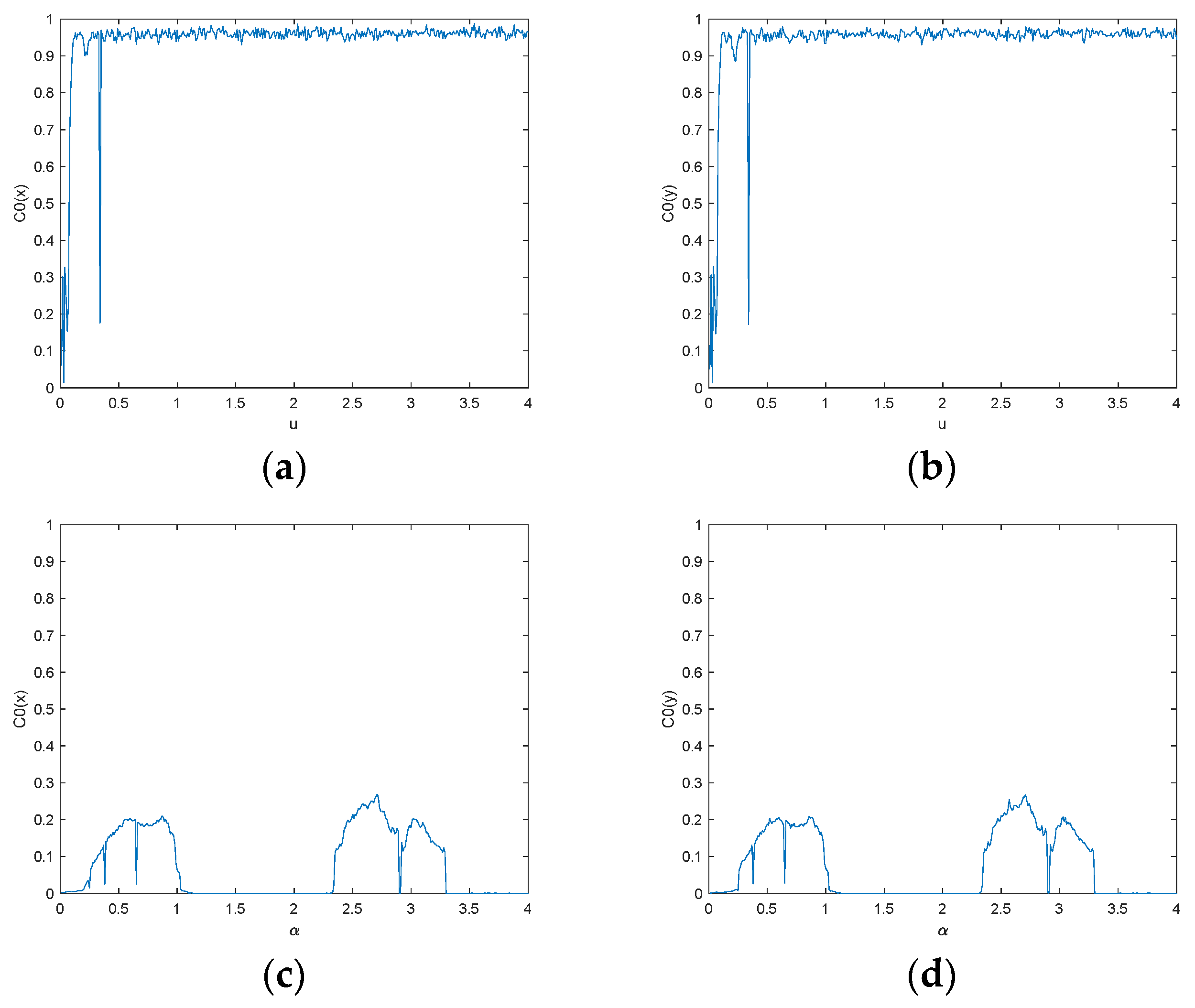
The main idea of the C₀ complexity algorithm is to split the sequence into regular and irregular parts and what is wanted is the percentage of the irregular part of the whole chaotic sequence. The specific calculation steps of the C₀ complexity algorithm are as follows.

• Discrete FFT transform of the sequence $\psi (n)$ by Equation (13)

  $$\Psi (s)={\displaystyle \sum _{n=0}^{N-1}\psi (n)e^{-j\frac{2\pi }{N}ns}}={\displaystyle \sum _{n=0}^{N-1}\psi (n)W_N^{ns}}$$

  (13)

  wherein s = 0, 1, 2, …, N − 1.
• Removing the irregular part of Ψ(s), assume that the mean square value of {Ψ(s), s = 0, 1, 2, …, N − 1} is Equation (14)

  $$Q_N=\frac{1}{N}{\displaystyle \sum _{s=0}^{N-1}|\Psi (s){|}^2}$$

  (14)
• Adding a parameter η to the above equation and leaving more than η multiple of that mean square value, assuming the value of the remaining part is zero, i.e.,

  $$\tilde{\Psi }(s)= \left\{\begin{array}{c}\Psi (s),\\ 0,\end{array}\right.\begin{array}{c}|\Psi (s){|}^2>\eta Q_N\\ |\Psi (s){|}^2<\eta Q_N\end{array}$$

  (15)
• Fourier inversion of Equation (15) by Equation (16)

  $$\tilde{\psi }(n)=\frac{1}{N}{\displaystyle \sum _{s=0}^{N-1}\tilde{\Psi }(s)e^{j\frac{2\pi }{N}ns}}=\frac{1}{N}{\displaystyle \sum _{s=0}^{N-1}\tilde{\Psi }(s)W_N^{-ns}}$$

  (16)

  wherein n = 0, 1, 2, …, N − 1.
• The expression of the C₀ complexity measure is Equation (17)

  $$C_0(\eta ,N)=\frac{1}{{\displaystyle \sum _{n=0}^{N-1}|\psi (n)}{|}^2}{\displaystyle \sum _{n=0}^{N-1}|\psi (n)}-\tilde{\psi }(n){|}^2$$

  (17)

The C₀ complexity algorithm developed based on the FFT transform removes the regular part and retains the irregular part. The more irregular parts in the whole sequence, the closer the corresponding time domain signal is to the random sequence.

Figure 5 implies the C₀ complexity algorithm of the 2D-SCLMS map and LSMCL. Figure 5a,c are the C₀ values of the x sequence generated by the 2D-SCLMS map and LSMCL respectively. Figure 5b,d are the C₀ values of the y sequence generated by the 2D-SCLMS map and LSMCL respectively. When u > 0.35, the C₀ value of 2D-SCLMS map is very close to 1. However, the C₀ values of LSMCL are small. This indicates that 2D-SCLMS system has a high complexity, that is, the two sequences generated by 2D-SCLMS map are close to random sequences.

Figure 5. C₀ complexity algorithm. (a) 2D-SCLMS with u–C₀(x); (b) 2D-SCLMS with u–C₀(y); (c) LSMCL with β = 3, α–C₀(x); (d) LSMCL with β = 3, α–C₀(y).

3.2.5. 0–1 Test

The 0–1 test [31] is an reliable and useful binary algorithm to determine whether a system is chaotic or not, proposed by Gottwald and Melbourne [32]. The 0–1 test is a direct method to determine whether a system is chaotic or not by calculating whether the linear growth rate K_c values of the discrete data transformation variables are close to 1 or 0, without the need of phase space reconstruction.

For a sequence φ(s) of length M and any real constant ζ, define two equations,

$$p(s)={\displaystyle \sum _{i=1}^s\phi (i)}\cos (i\zeta )$$

(18)

$$q(s)={\displaystyle \sum _{i=1}^s\phi (i)}\sin (i\zeta )$$

(19)

where s = 1, 2, …, M.

According to Equations (18) and (19), the expression of the displacement mean squared error is Equation (20)

$$Q(s)=\underset{M\to \infty }{\lim }\frac{1}{M}{\displaystyle \sum _{i=1}^s{[p(i)-p(i+s)]}^2}+{[q(i)-q(i+s)]}^2$$

(20)

where s = 1, 2, …, M.

It can be seen that it increases linearly with time or that it is bounded, especially, if p(s)(q(s)) is Brownian motion, which implies that Q(s) increases linearly with time. If p(s)(q(s)) is bounded, which implies that Q(s) is also bounded. Finally, the expression for K_c is Equation (21)

$$K_c=\underset{s\to \infty }{\lim }\frac{\log Q(s)}{\log s}$$

(21)

A dynamical system is considered non-chaotic when K_c ≈ 0 and chaotic when K_c ≈ 1.

For the 2D-SCLMS map, when setting the parameter u = 3 and the initial values x₀ = 0.1 and y₀ = 0.5, the 0–1 test is performed for each of the two sequences generated by the 2D-SCLMS system. We obtain the test results of the (p,q) plot, as shown in Figure 6. The results show that both sequence trajectories are similar to Brownian motion. Moreover, when 0 ≤ u ≤ 3, the K_c values of both sequences are close to 1. Therefore, the 2D-SCLMS map is a chaotic system.

Figure 6. 0–1 test. (a) p(x)–q(x); (b) s–Q(x); (c) p(y)–q(y); (d) s–Q(y); (e) u–K_c(x); (f) u–K_c(y).

3.2.6. Sample Entropy

A method to assess the complexity of a system is sample entropy. For a sequence U = {u(1), u(2), …, u(N)}, define parameters s, v.

Reconstructing s dimensional vectors V(1), V(2), …, V(N-s + 1), where V(i) = [u(i), u(i + 1), …, u(i + s − 1)]

$$H_i^s=\frac{H}{N-s}$$

(22)

where H is the number of V(i)’s that satisfy the condition d[V(i), V(j)] ≤ v

Find the average of the above equation for all i

$$H^s(\upsilon )=\frac{{\displaystyle \sum _{i=1}^{N-s+1}{H}_i^s(\upsilon )}}{N-s+1}$$

(23)

Set g = s + 1, repeating the above steps, we get D^g(v)

Then, the sample entropy is defined as

$$SampEn=-\ln \frac{D^g(\upsilon )}{H^s(\upsilon )}$$

(24)

Figure 7 implies the sample entropy of two sequences generated by the 2D-SCLMS map separately. When u > 0.35, the sample entropy is close to 2, which indicates that the two sequences are chaotic sequences and the 2D-SCLMS map is a complex chaotic system.

Figure 7. Sample entropy. (a) u–SampEn(x); (b) u–SampEn(y).

3.2.7. Permutation Entropy

A valid way to test the complexity of chaotic sequences is permutation entropy (PE) [33]. The range of PE is from 0 to 1. A larger PE indicates that the generated chaotic sequence is more complex.

In Figure 8, the PE value is very close to 1, which explains that the 2D-SCLMS system is a complex chaotic system.

Figure 8. Permutation entropy.

In summary, this paper proposes a hyperchaotic system based on two existing chaotic maps, which has a larger parameter space and better chaotic properties than some existing chaotic maps. Based on this, the hyperchaotic system can be applied to encryption to provide convenience and security for image transmission. Therefore, a new symmetric image encryption algorithm based on this system is proposed in the paper.

4. Pixel Scrambling

Two matrices A, B are arranged in ascending order by columns to produce two position index matrices A₁, B₁. Let A₁ be the row index and B₁ be the column index, combined together to permute the matrix P. In this section, the 6 × 6 matrix is used as an example and the results are shown in Figure 9.

$$[~,A_1]=sort(A)$$

(25)

$$[~,B_1]=sort(B)$$

(26)

$$P_1=scramble(P,[A_1,B_1])$$

(27)

Figure 9. Pixel scrambling.

5. Image Encryption Algorithm

The paper expounds the symmetric encryption scenario based on 2D-LSCM and new 2D-SCLMS system and Figure 10 is the flowchart. The encryption step mainly includes pixel scrambling, Xnor, and diffusion.

Figure 10. The encryption flowchart.

• Generation of keys

To heighten the safety of the scenario and the relevance of keys to original image. The hash is utilized to create initial parameters of the two systems. The hash 384 algorithm is used to acquire a 384-bit hash value that can be converted into a sequence of 48 binary values k₁, k₂, …, k₄₈. These values are computed by Equation (28)

$$\left\{\begin{array}{c}{x}_0=mod\left(\left(k_1+k_2+k_3+k_4+k_5+k_6+k_7+k_8+k_9+k_{10}\right),256\right)/256+x_0^{\prime }\hfill \\ y_0=mod\left(\left(k_{11}+k_{12}+k_{13}+k_{14}+k_{15}+k_{16}+k_{17}+k_{18}+k_{19}+k_{20}\right),256\right)/256+y_0^{\prime }\hfill \\ u=mod\left(\left(k_{21}+k_{22}+k_{23}+k_{24}+k_{25}+k_{26}+k_{27}+k_{28}+k_{29}+k_{30}\right),256\right)/256+u^{\prime }\hfill \\ z_0=mod\left(\left(k_{31}+k_{32}+k_{33}+k_{34}+k_{35}+k_{36}\right),256\right)/256+z_0^{\prime }\hfill \\ w_0=mod\left(\left(k_{37}+k_{38}+k_{39}+k_{40}+k_{41}+k_{42}\right),256\right)/256+w_0^{\prime }\hfill \\ \alpha =mod\left(\left(k_{43}+k_{44}+k_{45}+k_{46}+k_{47}+k_{48}\right),256\right)/256+{\alpha }^{\prime }\hfill \end{array}\right.$$

(28)

where the parameters x₀′, y₀′, u′, z₀′, w₀′, α′ are symmetric keys.

2.

Pixel scrambling

The initial values (x₀, y₀, u) are brought into the 2D-SCLMS map for MN + 500 iterations to generate two chaotic sequences x_n, y_n. The first 500 iterations are discarded in order to eliminate transient effects. First, the two sequences are processed separately to obtain two new sequences U, V.

$$\begin{array}{l}{u}_i=floor(mod(x_i\times {10}^{10},256))\\ v_i=floor(mod(y_i\times {10}^{10},256))\end{array}$$

(29)

U, V sequences are converted to matrices U₁, V₁ respectively. The sequence U₁, V₁ are sorted in ascending order by each column to generate two position indexes L₁, L₂. As introduced in Section 4, let L₁ be the row index and L₂ be the column index, and combine them together to disrupt the original image matrix P to generate P₁.

3.

Xnor

Perform the Xnor operation on matrix P₁ and matrix V₁ to generate matrix P₂.

$$P_2=255-\mathrm{mod}(bitxor(V_1,P_1),256)$$

(30)

4.

Diffusion of rows

The initial values (z₀, w₀, α) are brought into the 2D-LSCM for MN + 500 iterations to generate two chaotic sequences z_n, w_n. The first 500 iterations are discarded in order to eliminate transient effects.

$$\begin{array}{l}{a}_i=round(mod(z_i\times {10}^{14},256))\\ b_i=ceil(mod(w_i\times {10}^{14},256))\end{array}$$

(31)

A, B sequences are converted to matrices Z₂, W₂ respectively.

For the first column of P₂, P₃(i, 1) is calculated via Equation (32)

$$P_3(i,1)=\mathrm{mod}(P_2(i,1)+P_2(i,N)+Z_2(i,1),256)$$

(32)

For the other column of P₂, P₃(i, j) is calculated using Equation (33)

$$P_3(i,j)=\mathrm{mod}(P_2(i,j)+P_3(i,j-1)+Z_2(i,j),256)$$

(33)

5.

Diffusion of columns

For the first row of P₃, P₄(1, j) is calculated by Equation (34)

$$P_4(1,j)=\mathrm{mod}(P_3(1,j)+P_3(M,j)+W_2(1,j),256)$$

(34)

For the other column of P₃, P₄(i, j) is calculated by Equation (35)

$$P_4(i,j)=\mathrm{mod}(P_3(i,j)+P_4(i-1,j)+W_2(i,j),256)$$

(35)

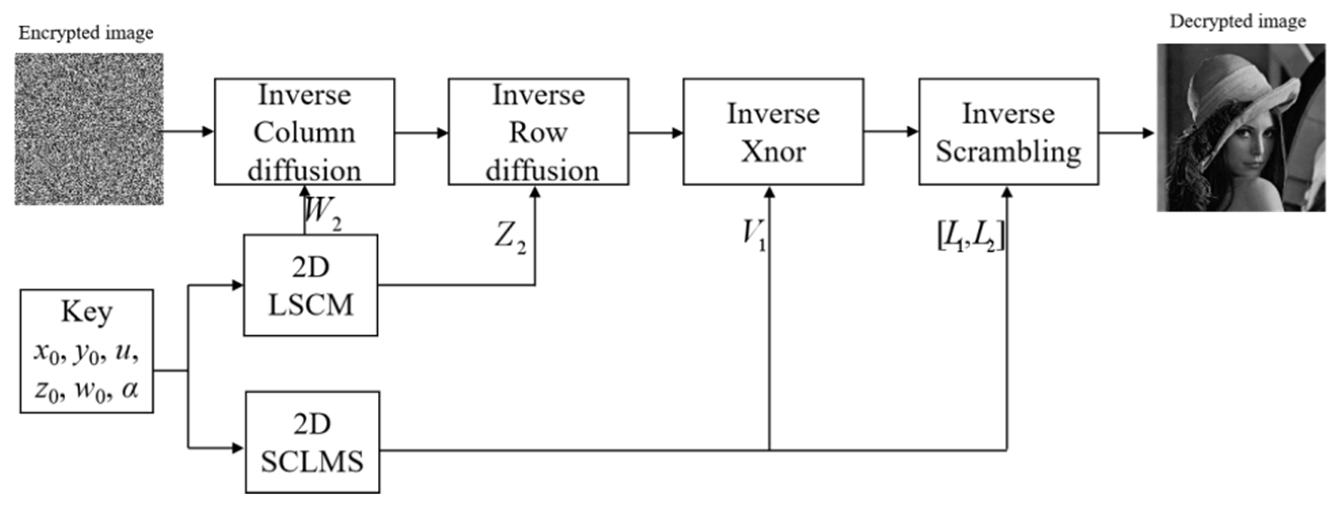
6. Image Decryption

The specific step is described below and drawn in Figure 11.

Figure 11. The decryption flowchart.

The image is obtained by performing the inverse operations of column diffusion, row diffusion, Xnor, and pixel scrambling on the ciphertext image in turn.

7. Experimental Results and Performance Analysis

To confirm the performance of the new symmetric encryption programme, all experiments are conducted on a PC with AMD Ryzen 2.00 GHz CPU, 8 G RAM, and 1 TB hard disk with Window 10 Ultimate system. This experiment is operated by MATLAB R2020a software. The selected images in this paper are all 512 × 512 in size.

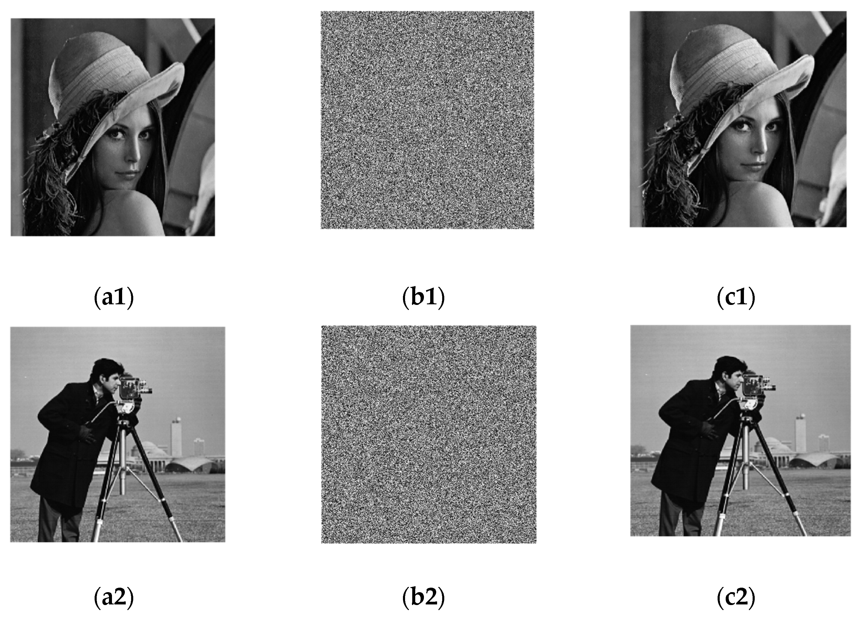
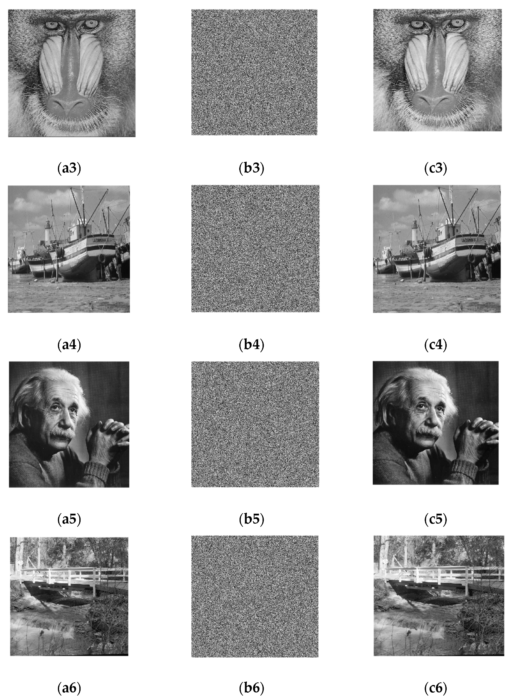
7.1. Simulation Results

In this paper, we set the parameters x₀′, y₀′, z₀′, w₀′, and α′ all to 0 and u’ = 1. Six images are selected for testing. In Figure 12, each column is respectively the original, ciphertext and decrypted image. All the cipher images resemble noise and all of them can be decrypted successfully, which illustrates that the encryption algorithm is extremely secure.

Figure 12. Illustration of image encryptions and decryptions. (a1–a6) Plain images; (b1–b6) Encrypted images; (c1–c6) Decrypted images.

7.2. Running Time (Complexity)

To verify that the new encryption scheme is practical and efficient, we calculated the time for the encryption algorithm and the decryption algorithm in Table 1. Table 1 demonstrates that the new encryption algorithm takes less time, which illustrates that the algorithm is practical and efficient. Table 2 shows the running time comparison between the encryption algorithm proposed in this paper and other encryption algorithms. It can be seen from Table 2 that the scheme proposed in this paper has an acceptable speed.

Table 1. Running time of encryption and decryption algorithms (unit: s).

Image	Lena	Couple	Cattle	Boat	Average
Encryption	0.5769	0.5858	0.6556	0.6426	0.615225
Decryption	0.6137	0.6136	0.6352	0.6519	0.6286

Table 2. The average running time of different encryption schemes (unit: s).

Scheme	Encryption Time	Microprocessor/RAM/O.S
Ref. [41]	11.005	2.53 GHz, 2 GB RAM, Windows 7 and Matlab R2012b
Ref. [42]	0.497	1.9 GHz, 4 GB RAM, Windows 7 and MATLAB 7.9
Ours	0.615	2.00 GHz, 8 GB RAM and 1 TB hard disk with, Window 10 and MATLAB R2020a

7.3. Information Entropy (IE)

Shannon proposed the entropy criterion in [43]. It is an indispensable tool [44] for testing the randomness of images before and after encryption. The expression of information entropy [45] is

$$H(s)=-{\displaystyle \sum _{i=0}^{2^8-1}p(s_i){\log }_{2}p(s_i)}$$

(36)

In Equation (36), p(s_i) is the probability of s_i. Theoretically, the ideal value of IE is 8.

We test the IE of the new encryption scenario and compare it with other encryption algorithms on “Boat” image. For the IE, Table 3 demonstrates that the original image is around 7, while the encrypted image is almost nearly 8. Table 4 demonstrates that our scheme has the largest entropy value, which explains that the ciphertext image has better randomness.

Table 3. IE of multiple images.

Image	Lena	Couple	Cameraman	Boat	Einstein	Cattle
Plain	7.3920	7.2010	7.0480	7.1914	7.2655	7.3579
Encryption	7.9994	7.9993	7.9994	7.9993	7.9993	7.9993

Table 4. IE of different schemes.

Image	Ref. [27]	Ref. [41]	Ref. [42]	Ours
Boat	7.9959	7.99928	7.9980	7.9993

7.4. Key Space Analysis

An excellent encryption scenario with a key space greater than 2¹⁰⁰ is considered sufficient to oppose the most usual violent attack [46]. Then, the key of this scenario consists of a 384-bit hash values and initial keys x₀′, y₀′, u′, z₀′, w₀′, α′. Suppose the calculation accuracy is 10⁻¹⁴, the key space of this algorithm is 10^14×6 = 10⁸⁴. In addition to that, we have the 384-bit stream generated by SHA-384, so the entire key space is resistant to violent attack.

7.5. Key Sensitivity Analysis

A slight change of key causes the decrypted image to be completely different. We encrypt the “Boat” using the correct key. After that, any one of these keys is changed slightly. Figure 13 displays the images under different key decryption. When keys change very little, the decrypted images resemble noise, which indicates that this scenario is extremely sensitive to all keys.

Figure 13. Key sensitivity analysis. (a) Image decrypted with correct keys; (b) Decrypted image when x₀′ changes to x₀′ + 10⁻⁹; (c) Decrypted image when y₀′ changes to y₀′ + 10⁻⁹; (d) Decrypted image when u′ changes to u′ + 10⁻⁹; (e) Decrypted image when z₀′ changes to z₀′ + 10⁻⁹; (f) Decrypted image when w₀′ changes to w₀′ + 10⁻⁹.

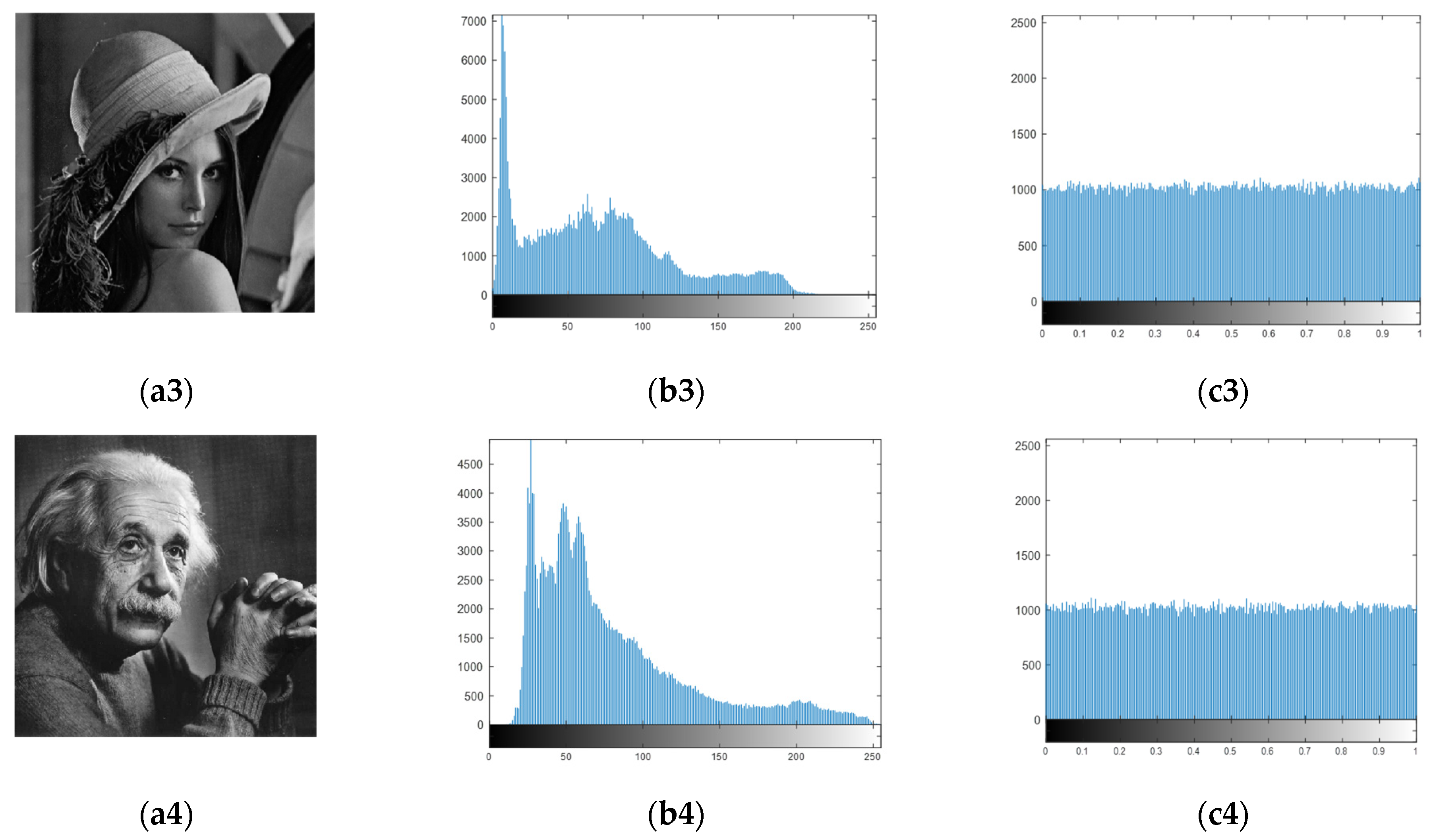
7.6. Histogram Analysis

Normally, the histogram is nearly flat to resist statistical attacks. Obviously, the histogram of ciphertext images tends to be uniformly distributed in Figure 14, which indicates that this scenario is resistant to statistical attacks.

Figure 14. Histogram analysis. (a1–a4) Plain images; (b1–b4) Plain image histograms; (c1–c4) Encrypted image histograms.

7.7. Chi-Square Analysis

This paper utilizes a quantitative way to calculate the resistance of encryption scenario to statistical attacks, i.e., the chi-square test [47], whose expression is Equation (37).

$${\chi }^2={\displaystyle \sum _{i=0}^{255}\frac{{({\upsilon }_i-{\upsilon }_0)}^2}{{\upsilon }_0}}$$

(37)

where υ_i is frequency occupied by grayscale value i. υ₀ = MN/256. Table 5 shows the chi-square calculation results, where the first and second rows show the chi-square results of the encrypted and plain images, respectively. The chi-square of all encrypted images is less than 293.25 [34], which indicates that the encryption scheme is sufficient to defend against statistical attacks.

Table 5. Chi-square.

Image	Lena	Couple	5.2.10	Cattle	Boat
Chi-square	232.9199	261.8418	229.6328	262.5801	259.3848
	270,681.8	298,865.2	118,561.8	187,692.2	383,969.7

7.8. Correlation Analysis

The meaning of encryption is to decrease the correlation, which is expressed in Equations (38)–(41). This section arbitrarily selects 10,000 pairs of adjacent pixels x, y from the plain and encrypted images and calculates them in horizontal, vertical, and diagonal directions.

$${\rho }_{xy}=\frac{1}{\sqrt{D(x)D(y)}}cov(x,y)$$

(38)

$$\mathrm{cov}(x,y)=\frac{1}{N}{\displaystyle \sum _{i=1}^N(x_i-E(x))(y_i-E(y))}$$

(39)

$$E(x)=\frac{1}{N}{\displaystyle \sum _{i=1}^N{x}_i}$$

(40)

$$D(x)=\frac{1}{N}{\displaystyle \sum _{i=1}^N{(x_i-E(x))}^2}$$

(41)

Table 6 lists the correlation coefficients of multiple images. Table 7 compares the correlation coefficients of different encryption algorithms for the “Boat” image. Figure 15 reveals the correlation of the plain and ciphertext images of “Lena”. The correlation of the plain image is diagonal in all directions, i.e., the correlation of the original image is very high. The correlation of the ciphertext image is scattered throughout the image, that is, the correlation of the ciphertext image is vastly abated, which demonstrates that the encryption scenario is very good.

Table 6. Correlation coefficient of multiple images.

Image	Horizontal	Vertical	Diagonal
Lena	0.9840	0.9835	0.9717
	0.0037	−0.00027	0.001
Cameraman	0.9853	0.9870	0.9765
	0.0004	−0.00006	−0.00035
Boat	0.9833	0.9727	0.9617
	0.0012	0.000587	−0.00003
Couple	0.9624	0.9650	0.9386
	0.0046	−0.00062	0.000345
Einstein	0.9687	0.9644	0.9548
	−0.0049	0.0034	−0.0013
Cattle	0.8573	0.9103	0.8423
	0.0018	0.0031	0.000611

Table 7. Correlation coefficients of Boat for multiple algorithms.

Direction	Horizontal	Vertical	Diagonal
Ref. [27]	−0.0295	−0.015	−0.0224
Ref. [41]	0.009480	0.004406	−0.010305
Ref. [42]	−0.0100	−0.0124	−0.0185
Ours	0.0012	0.000587	−0.00003

Figure 15. Correlation. (a) Plain image horizontal correlation; (b) Plain image vertical correlation; (c) Plain image diagonal correlation; (d) Encrypted image horizontal correlation; (e) Encrypted image vertical correlation; (f) Encrypted image diagonal correlation.

7.9. Differential Attack Analysis

The value of pixel change rate (NPCR) [48,49] and the unified average change intensity (UACI) [50] are utilized to determine the ability of the new scheme against differential attacks, which are given by

$$\mathrm{N}\mathrm{P}\mathrm{C}\mathrm{R}=\frac{1}{M\times N}{\displaystyle \sum _{i=1}^M{\displaystyle \sum _{j=1}^N|Sign(C_1(i,j)-C_2(i,j))|}}$$

(42)

$$\mathrm{U}\mathrm{A}\mathrm{C}\mathrm{I}=\frac{1}{M\times N}{\displaystyle \sum _{i=1}^M{\displaystyle \sum _{j=1}^N\frac{|C_1(i,j)-C_2(i,j)|}{2^8-1}}}$$

(43)

The ideal NPCR and UACI values are respectively 0.996094 and 0.334635 for 256 gray level images [51,52]. Table 8 lists the NPCR and UACI values of the new scenario for several images and they are both approach desired value. The UACI of the new scenario is closer to 33.4635% than other algorithms in Table 9. Thus, this scenario is forceful against differential attacks.

Table 8. NPCR and UACI of multiple images.

Image	NPCR	UACI
Lena	0.996235	0.334444
Einstein	0.996117	0.334894
5.2.10	0.996239	0.334401
Cattle	0.996246	0.334874
Boat	0.995869	0.334856
Cameraman	0.996155	0.334441
Mean	0.9961435	0.3346517

Table 9. NPCR and UACI of Boat for different schemes.

	NPCR	UACI
Ref. [27]	0.996209	0.336018
Ref. [41]	0.996100	0.334412
Ref. [42]	0.996102	0.335367
Ours	0.995869	0.334856

7.10. Local Shannon Entropy

The local Shannon entropy can better express the randomness of the local image and can overcome some drawbacks of the global Shannon entropy. For each image P, arbitrarily choose k non-overlapping sub-images S_i, i = 1, 2, …, k. T_B pixels are arbitrarily chosen for every sub-image. The local Shannon information entropy is calculated as follows:

$$\overline{L{H}_{k,T_B}}(P)={\displaystyle \sum _{i=1}^k\frac{H(S_i)}{k}}$$

(44)

In Equation (44), H(S_i) shows the IE of sub-image S_i. We set k = 30, T_B = 7936 in this paper. When the confidence interval is 0.05, the local Shannon entropy is in the interval of [7.901901305, 7.903373329] [34]. Table 10 lists the local Shannon entropy of multiple images whose results pass the experiment, i.e., the randomness of the local image is good.

Table 10. Local Shannon entropy.

Image	Local Entropy	Result
Lena	7.9025	Pass
Cameraman	7.9027	Pass
Boat	7.9024	Pass
Cattle	7.9026	Pass
Einstein	7.9028	Pass
5.2.10	7.9027	Pass

7.11. Cropping Attack

Remove some pixels from the encrypted image and see if it can be decrypted is the cropping attack. In this section, we test “Lena”. Figure 16 presents the decrypted images after cutting 1/64, 1/16 and 1/4, respectively. Even if 1/4 of the data is cut off, the decrypted image still displays information from the original image, which illustrates that this scheme is highly resistant to clipping attack.

Figure 16. Cropping attack. (a) Crop 1/64; (b) Crop 1/16; (c) Crop 1/4; (d) Decrypted image of crop 1/64; (e) Decrypted image of crop 1/16; (f) Decrypted image of crop 1/4.

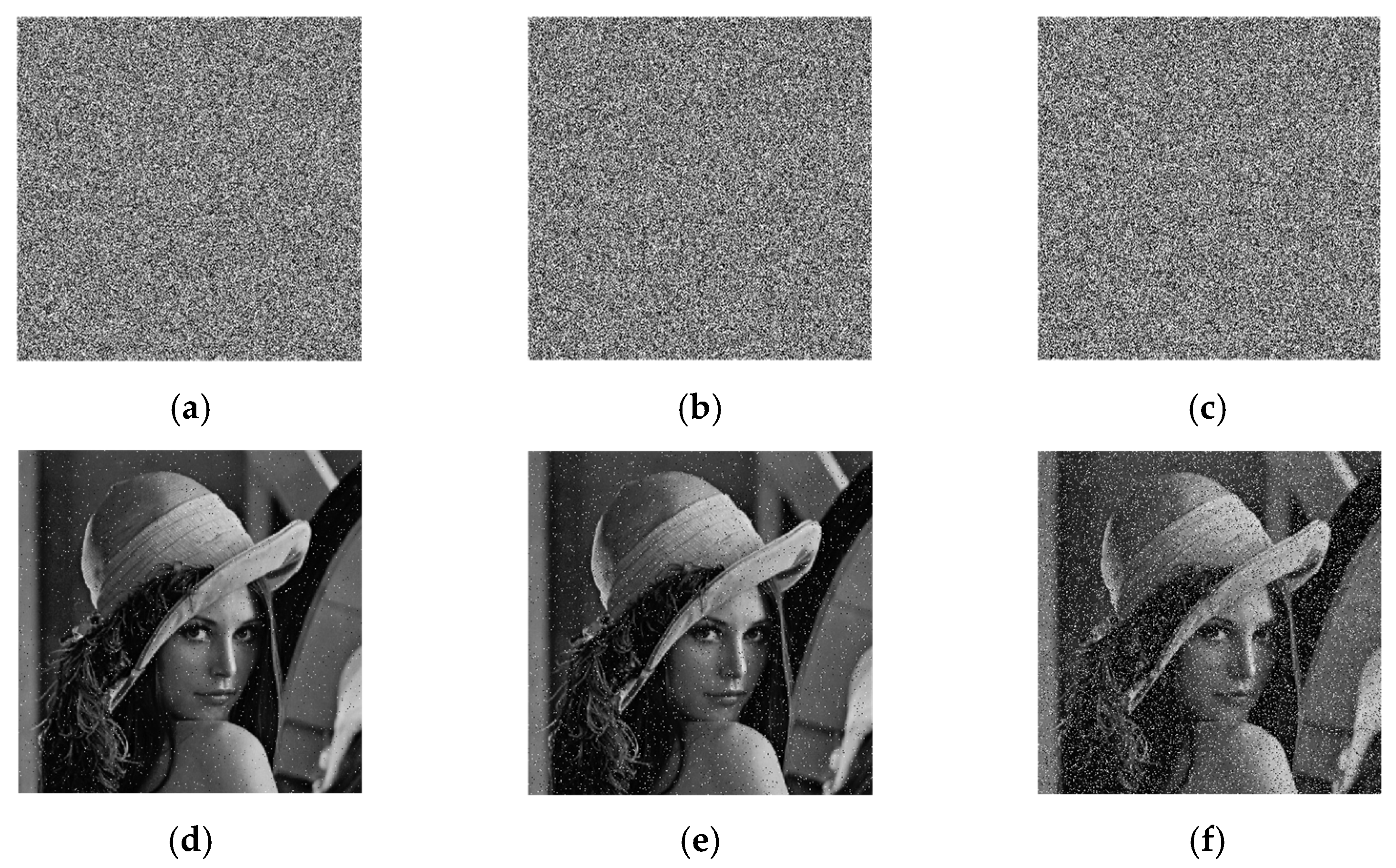
7.12. Noise Attack

Inevitably, images are affected during transmission by noise that causes data loss. We take the noise of pepper and salt as an example to show the robustness of the proposed encryption algorithm, whose noise strengths are 0.005, 0.01, and 0.05, respectively. Even with the addition of 0.05 noise, the decrypted image still displays information from the original image in Figure 17, which indicates that this scheme is highly resistant to noise attacks.

Figure 17. Noise attack. (a) 0.005 noise; (b) 0.01 noise; (c) 0.05 noise; (d) Decrypted image with 0.005 noise; (e) Decrypted image with 0.01 noise; (f) Decrypted image with 0.05 noise.

8. Color Image Encryption

The encryption algorithm proposed in this paper can be used not only for grayscale images, but also for color images. The flowchart of color image encryption is given in Figure 18. Unlike grayscale images, color images are divided into three channels, R, G, and B. Each channel is encrypted separately and finally combined to obtain the cipher image.

Figure 18. The color image encryption flowchart.

We take the “Peppers” image as an example. The original image, cipher image, and decrypted image are shown in Figure 19. From the figure, we can see that the cipher image is similar to noise, and no information from the original image is obtained. This indicates that the encryption algorithm proposed in this paper works well and is applicable to color images.

Figure 19. Color image. (a) Plain image; (b) Cipher image; (c) Decrypted image.

When the color image is divided into three channels, R, G, and B, the encryption of each channel is the same as that of the gray image. Therefore, the security tests are not re-demonstrated in detail.

9. Application Areas of Encryption Algorithms

The high efficiency and securer performance of the proposed symmetric encryption algorithm make it possible to apply in many military, commercial, and even daily-use fields. Herein, we itemize several typical applications.

• E-mail

Image data in e-mails are usually transmitted over non-secure channels, such as the Internet. The widespread use of the Internet has also made encrypting e-mail with sensitive information a very important application in recent years.

2.

Electronic money

Electronic money, as a new means of financial transactions, must make the transactions authenticated but untraceable. Transactions must be authenticated so that both parties involved in the transaction are not deceived. Transactions must be untraceable so that each party’s privacy is protected. In practice, however, if there is no special protocol to support collaboratively, these requirements are difficult to achieve.

3.

Authentication server

The authentication server solves the security problem between two communities at different endpoints in the network. Two groups must be able to exchange keys, and at the same time must ensure that they are talking to the correct counterparty, not an imposter. The authentication server implements these functions through various protocols that rely on encryption mechanisms.

4.

Smart card

A smart card contains a microcomputer as well as a small amount of storage space. In general, smart cards are mostly used on various forms of credit. Other types of smart cards are used for access to computers or building access control, etc. Smart cards use encryption technology because it allows certain important operations to be performed, such as modifying bank accounts and accessing secure environments.

5.

Internet of Things

In the Internet of Things, the use of smart mobile devices to transfer images in large amounts of data has become increasingly common, such as photos of criminal suspects, medical photos of patients, military photos, etc. The image data captured by some end devices or IoT nodes is related to the private information of users. To protect these image data, image encryption schemes provide a convenient and secure method for the confidentiality of image conversion and storage in IoT systems.

10. Conclusions

The paper mainly introduces a new 2D-SCLMS map based on Logistic and Sine maps. A series of tests, such as Lyapunov exponent, 0–1 test, two complexity analysis methods, and two entropy analysis methods, are used to conclude that the 2D-SCLMS map is hyperchaotic with a broader chaotic range and better randomness. This paper further designs a symmetric image encryption algorithm using 2D-SCLMS map and 2D-LSCM. The encryption algorithm is used under the permutation-diffusion framework which combines pixel scrambling, Xnor, and diffusion. In addition, it uses the hash to create the initial parameters of two systems, which greatly improves the resistance to known plaintext and chosen plaintext attacks. Finally, the simulation experiments of time complexity, key space and sensitivity, information entropy and local Shannon entropy and correlation coefficient demonstrate the large key space, high security, and low time complexity of the new encryption scheme.

Among them, the information entropy of encrypted images using the proposed encryption algorithm can reach 7.9994 at best, which is very close to 8 and better than other related algorithms. The correlation coefficient of the cipher image can even reach −0.00003, which is far smaller than the correlation coefficients obtained using other encryption algorithms. Besides, various attacks, e.g., differential, cropping, and noise attacks, are also analyzed and the conclusions illustrate that this algorithm is also resistant to various attacks. Finally, the value of UACI can reach 33.4651%, which is very small from the standard value and can still recover the original image well when a quarter of the image is cropped off.

In the future, we intend to focus on the verification of the hyperchaotic systems from the perspective of theoretical analysis. Moreover, we remain interested in the practical combination of the proposed image encryption schemes with Internet of Things applications to effectively protect the security of images during the transmission of Internet of Things.