Convergence Analysis of the LDG Method for Singularly Perturbed Reaction-Diffusion Problems

Abstract

We analyse the local discontinuous Galerkin (LDG) method for two-dimensional singularly perturbed reaction–diffusion problems. A class of layer-adapted meshes, including Shishkin- and Bakhvalov-type meshes, is discussed within a general framework. Local projections and their approximation properties on anisotropic meshes are used to derive error estimates for energy and “balanced” norms. Here, the energy norm is naturally derived from the bilinear form of LDG formulation and the “balanced” norm is artificially introduced to capture the boundary layer contribution. We establish a uniform convergence of order k for the LDG method using the balanced norm with the local weighted $L^2$ projection as well as an optimal convergence of order $k+1$ for the energy norm using the local Gauss–Radau projections. The numerical method, the layer structure as well as the used adaptive meshes are all discussed in a symmetry way. Numerical experiments are presented.

1. Introduction

Over the past few decades, singularly perturbed problems have attracted considerable attention in the scientific community. Such problems arise in many applications, including the modelling of viscous fluid flows, semiconductor devices, and more [1]. For reaction–diffusion problems, difficulties arise owing to the presence of boundary layers in the solution. Unless the meshes are sufficiently refined, traditional finite-difference or finite-element methods on uniform or quasi-uniform meshes yield oscillatory and inaccurate numerical solutions. Consequently, three common approaches have been proposed in the literature. The first is to use traditional numerical methods on strongly refined, layer-adapted meshes, such as the Shishkin-type (S-type) or Bakhvalov-type (B-type) mesh [2,3,4,5]. Various parameter-uniform convergence results have been established in this way; notably, the order of convergence and error constant are independent of the singular perturbation parameters. The second approach is to use a stabilised numerical method, such as the streamline diffusion finite-element method, interior-penalty discontinuous Galerkin method, or local discontinuous Galerkin (LDG) method [6,7,8]; well-behaved local error estimates have been investigated using uniform or quasi-uniform meshes. The third approach [2,9,10,11] is to combine the aforementioned stabilised numerical methods with layer-adapted meshes. From a practical perspective, the third approach is preferable because it is more stable and less sensitive to the choice of transition point on the layer-adapted mesh.

The LDG method is a form of finite-element method; it was first proposed as a generalisation of the discontinuous Galerkin (DG) method for a convection–diffusion problem [12]. Later, it was applied to solve the purely elliptic problem [13], convection–diffusion problems [14], Stokes system [15], KdV-type equations [16], Hamilton–Jacobi equations [17], time-dependent fourth-order problems [18] and other higher-order partial differential equations [19]. Because the LDG method shares many advantages of the DG methods and can effectively simulate the acute change of a singular solution, it is particularly suited to solving singularly perturbed problems. For example, Cheng et al. performed double-optimal local error estimates for two explicit, fully discrete LDG methods on quasi-uniform meshes [6,7]. Xie et al. established uniform convergence and super-convergence analyses of the LDG method on a standard Shishkin mesh [10,11,20]. However, few results have been established for the LDG method on general S-type or B-type meshes.

Recently, we analysed the LDG method on several S-type meshes and a B-type mesh for singularly perturbed convection–diffusion problems. Robust error estimates were derived from the energy norm [9]. However, the reaction–diffusion case remains unexplored. Despite its simpler appearance, reaction-dominated diffusion without convection differs from convection–diffusion in the following three respects:

• For singularly perturbed reaction–diffusion problems, the boundary layer structure is considerably more complicated because of the parabolic layers along all boundary edges [21]. As a result, the regularity of the solution is complex. This adds many difficulties to the theoretical analysis, such as in the construction of layer-adapted meshes and the estimates of various approximation errors.
• Better than the convergence order obtained in [9] for the convection–diffusion problem, we can establish an optimal convergence of order $k+1$ for the LDG method in the energy norm through a more elaborate analysis for the two-dimensional Gauss–Radau projections on anisotropic meshes.
• In the reaction–diffusion region, the balanced-norm is more suitable to reflect the contribution of the boundary layer component [22]. To date, balanced-norm error estimates are only available for the Galerkin finite-element method (FEM) [23,24], mixed FEM [22], and hp-FEM [25], but not for the LDG method. For the first time, we establish the uniform convergence of the LDG method for the balanced norm.

Note that the numerical method, layer structure as well as the used adaptive meshes are all discussed in a symmetry way, which simplify our analysis to some extent.

The remainder of this paper is organised as follows. In Section 2, we describe the LDG method. In Section 3, we introduce a class of layer-adapted meshes and state some elementary lemmas for them. In Section 4, we establish uniform convergence for the balanced and energy norms. In Section 5, we present numerical experiments.

2. The LDG Method

Consider a two-dimensional singularly perturbed reaction–diffusion problem, expressed as

$$\begin{array}{cccc}\hfill -\epsilon \mathsf{\Delta }u+b(x,y)u& =f(x,y),\hfill & \hfill \mathrm{in}& \mathsf{\Omega }={(0,1)}^2,\hfill \end{array}$$

(1a)

$$\begin{array}{cccc}\hfill u& =0,\hfill & \hfill \mathrm{on}& \partial \mathsf{\Omega },\hfill \end{array}$$

(1b)

where $0<\epsilon \ll 1$ is a perturbation parameter, and $b(x,y)\ge 2{\beta }^2>0$ for any $(x,y)\in \overline{\mathsf{\Omega }}$ and for some positive constant $\beta$. In this section, we present the LDG method for (1).

Let ${\mathsf{\Omega }}_N={\left\{K_{ij}\right\}}_{i=1,2,\dots ,N_x}^{j=1,2,\dots ,N_y}$ be a rectangle partition of $\mathsf{\Omega }$ with element $K_{ij}=I_i\times J_j$, where $I_i=(x_{i-1},x_i)$ and $J_j=(y_{j-1},y_j)$. We set $h_{x,i}=x_i-x_{i-1}$, $h_{y,j}=y_j-y_{j-1}$, and $\hslash ={min}_{K_{ij}\in {\mathsf{\Omega }}_N}min\{h_{x,i},h_{y,j}\}$. We let

$${\mathcal{V}}_N=\{v\in L^2(\mathsf{\Omega }):v{|}_K\in {\mathcal{Q}}^k(K),K\in {\mathsf{\Omega }}_N\},$$

(2)

be the discontinuous finite-element space, where ${\mathcal{Q}}^k(K)$ represents the space of polynomials on K with a maximum degree of k in each variable. ${\mathcal{V}}_N$ is contained in a broken Sobolev space, expressed as

$${\mathcal{H}}^1({\mathsf{\Omega }}_N)=\{v\in L^2(\mathsf{\Omega }):v{|}_K\in H^1(K),K\in {\mathsf{\Omega }}_N\},$$

(3)

whose function is allowed to have discontinuities across element interfaces. For $v\in {\mathcal{H}}^1({\mathsf{\Omega }}_N)$ and $y\in J_j$, $j=1,2,\dots ,N_y$, we use $v_{i,y}^{\pm }={lim}_{x\to x_i^{\pm }}v(x,y)$ and $v_{x,j}^{\pm }={lim}_{y\to y_j^{\pm }}v(x,y)$ to express the traces evaluated from the four directions. We denote

$$\begin{array}{cc}\hfill {\left[\left[v\right]\right]}_{i,y}& =v_{i,y}^{+}-v_{i,y}^{-},\mathrm{for}i=1,2,\dots ,N_x-1,{\left[\left[v\right]\right]}_{0,y}=v_{0,y}^{+},{\left[\left[v\right]\right]}_{N_x,y}=-v_{N_x,y}^{-},\hfill \\ \hfill {\left[\left[v\right]\right]}_{x,j}& =v_{x,j}^{+}-v_{x,j}^{-},\mathrm{for}j=1,2,\dots ,N_y-1,{\left[\left[v\right]\right]}_{x,0}=v_{x,0}^{+},{\left[\left[v\right]\right]}_{x,N_y}=-v_{x,N_y}^{-},\hfill \end{array}$$

as the jumps on the vertical and horizontal edges, respectively.

Rewrite (1) into an equivalent first-order system:

$$\begin{array}{c}\hfill -p_x-q_y+bu=f,{\epsilon }^{-1}p=u_x,{\epsilon }^{-1}q=u_y,\mathrm{in}\mathsf{\Omega }.\end{array}$$

(4)

Let ${⟨·,·⟩}_D$ be the inner product in $L^2(D)$. In order to determine the approximate solution $\mathsf{𝕨}=(\mathsf{𝕦},\mathsf{𝕡},\mathsf{𝕢})\in {\mathcal{V}}_N^3\equiv {\mathcal{V}}_N\times {\mathcal{V}}_N\times {\mathcal{V}}_N$, we first multiply each of the Equation (4) by arbitrary smooth functions $v,s,r$, respectively, and integrating over $K_{ij}$, we get after a simple formal integration by parts in (4),

$$\begin{array}{cc}\hfill & {⟨p,v_x⟩}_{K_{ij}}-{⟨p_{i,y},v_{i,y}^{-}⟩}_{J_j}+{⟨p_{i-1,y},v_{i-1,y}^{+}⟩}_{J_j}\hfill \\ \hfill & +{⟨q,v_y⟩}_{K_{ij}}-{⟨q_{x,j},v_{x,j}^{-}⟩}_{I_i}+{⟨q_{x,j-1},v_{x,j-1}^{+}⟩}_{I_i}+{⟨bu,v⟩}_{K_{ij}}={⟨f,v⟩}_{K_{ij}},\hfill \\ \hfill & {\epsilon }^{-1}{⟨p,s⟩}_{K_{ij}}+{⟨u,s_x⟩}_{K_{ij}}-{⟨u_{i,y},s_{i,y}^{-}⟩}_{J_j}+{⟨u_{i-1,y},s_{i-1,y}^{+}⟩}_{J_j}=0,\hfill \\ \hfill & {\epsilon }^{-1}{⟨q,r⟩}_{K_{ij}}+{⟨u,r_y⟩}_{K_{ij}}-{⟨u_{x,j},r_{x,j}^{-}⟩}_{I_i}+{⟨u_{x,j-1},r_{x,j-1}^{+}⟩}_{I_i}=0.\hfill \end{array}$$

Next, we replace the smooth functions $v,s,r$ by test functions $\mathsf{𝕧},\mathsf{𝕤},\mathsf{𝕣}$, respectively, in the finite element space ${\mathcal{V}}_N$ and the exact solution $\mathit{w}=(u,p,q)$ by the approximate solution $\mathsf{𝕨}=(\mathsf{𝕦},\mathsf{𝕡},\mathsf{𝕢})$. As this function is discontinuous in each of its components, we must also replace the fluxes $u_{i,y},u_{x,j},p_{i,y},q_{x,j}$ by the numerical fluxes ${\widehat{\mathsf{𝕦}}}_{i,y}$, ${\widehat{\mathsf{𝕦}}}_{x,j}$, ${\widehat{\mathsf{𝕡}}}_{i,y}$, ${\widehat{\mathsf{𝕢}}}_{x,j}$. Then, the LDG scheme is defined as follows. Find $\mathsf{𝕨}=(\mathsf{𝕦},\mathsf{𝕡},\mathsf{𝕢})\in {\mathcal{V}}_N^3$ such that in each element $K_{ij}$, the variational forms

$$\begin{array}{cc}& {⟨\mathsf{𝕡},{\mathsf{𝕧}}_x⟩}_{K_{ij}}-{⟨{\widehat{\mathsf{𝕡}}}_{i,y},{\mathsf{𝕧}}_{i,y}^{-}⟩}_{J_j}+{⟨{\widehat{\mathsf{𝕡}}}_{i-1,y},{\mathsf{𝕧}}_{i-1,y}^{+}⟩}_{J_j}\hfill \end{array}$$

$$\begin{array}{cc}& +{⟨\mathsf{𝕢},{\mathsf{𝕧}}_y⟩}_{K_{ij}}-{⟨{\widehat{\mathsf{𝕢}}}_{x,j},{\mathsf{𝕧}}_{x,j}^{-}⟩}_{I_i}+{⟨{\widehat{\mathsf{𝕢}}}_{x,j-1},{\mathsf{𝕧}}_{x,j-1}^{+}⟩}_{I_i}+{⟨b\mathsf{𝕦},\mathsf{𝕧}⟩}_{K_{ij}}={⟨f,\mathsf{𝕧}⟩}_{K_{ij}},\hfill \end{array}$$

(5a)

$$\begin{array}{cc}& {\epsilon }^{-1}{⟨\mathsf{𝕡},\mathsf{𝕤}⟩}_{K_{ij}}+{⟨\mathsf{𝕦},{\mathsf{𝕤}}_x⟩}_{K_{ij}}-{⟨{\widehat{\mathsf{𝕦}}}_{i,y},{\mathsf{𝕤}}_{i,y}^{-}⟩}_{J_j}+{⟨{\widehat{\mathsf{𝕦}}}_{i-1,y},{\mathsf{𝕤}}_{i-1,y}^{+}⟩}_{J_j}=0,\hfill \end{array}$$

(5b)

$$\begin{array}{cc}& {\epsilon }^{-1}{⟨\mathsf{𝕢},\mathsf{𝕣}⟩}_{K_{ij}}+{⟨\mathsf{𝕦},{\mathsf{𝕣}}_y⟩}_{K_{ij}}-{⟨{\widehat{\mathsf{𝕦}}}_{x,j},{\mathsf{𝕣}}_{x,j}^{-}⟩}_{I_i}+{⟨{\widehat{\mathsf{𝕦}}}_{x,j-1},{\mathsf{𝕣}}_{x,j-1}^{+}⟩}_{I_i}=0,\hfill \end{array}$$

(5c)

hold for any $\mathsf{𝕫}=(\mathsf{𝕧},\mathsf{𝕤},\mathsf{𝕣})\in {\mathcal{V}}_N^3$, where

$$\begin{array}{cc}\hfill {\widehat{\mathsf{𝕡}}}_{i,y}& =\left\{\begin{array}{cc}{\mathsf{𝕡}}_{i,y}^{+}+{\lambda }_{i,y}{\left[\left[\mathsf{𝕦}\right]\right]}_{i,y},\hfill & i=0,1,\dots ,N_x-1,\hfill \\ {\mathsf{𝕡}}_{N_x,y}^{-}-{\lambda }_{N_x,y}{\mathsf{𝕦}}_{N_x,y}^{-},\hfill & i=N_x,\hfill \end{array}\right.\hfill \end{array}$$

(6a)

$$\begin{array}{cc}\hfill {\widehat{\mathsf{𝕦}}}_{i,y}& =\left\{\begin{array}{cc}0,\hfill & i=0,N_x,\hfill \\ {\mathsf{𝕦}}_{i,y}^{-},\hfill & i=1,2,\dots ,N_x-1,\hfill \end{array}\right.\hfill \end{array}$$

(6b)

for $y\in J_j$ and $j=1,2,\dots ,N_y$. Here, ${\lambda }_{i,y}\ge 0$ $(i=0,1,\dots ,N_x)$ are stabilisation parameters to be determined later. Analogously, for $x\in I_i$ and $i=1,2,\dots ,N_x$, we can define ${\widehat{\mathsf{𝕢}}}_{x,j}$ and ${\widehat{\mathsf{𝕦}}}_{x,j}$ for $j=0,1,\dots ,N_y$.

Write $⟨w,v⟩={\sum }_{K_{ij}\in {\mathsf{\Omega }}_N}{⟨w,v⟩}_{K_{ij}}$. Then, we write the above LDG method into a compact form: Find $\mathsf{𝕨}=(\mathsf{𝕦},\mathsf{𝕡},\mathsf{𝕢})\in {\mathcal{V}}_N^3$ such that

$$B(\mathsf{𝕨};\mathsf{𝕫})=⟨f,\mathsf{𝕧}⟩,\forall \mathsf{𝕫}=(\mathsf{𝕧},\mathsf{𝕤},\mathsf{𝕣})\in {\mathcal{V}}_N^3,$$

(7)

where

$$\begin{array}{cc}\hfill B(\mathsf{𝕨};\mathsf{𝕫})=& {\mathcal{T}}_1(\mathsf{𝕨};\mathsf{𝕫})+{\mathcal{T}}_2(\mathsf{𝕦};\mathsf{𝕫})+{\mathcal{T}}_3(\mathsf{𝕨};\mathsf{𝕧})+{\mathcal{T}}_4(\mathsf{𝕦};\mathsf{𝕧}),\hfill \end{array}$$

(8)

with

$$\begin{array}{cc}\hfill {\mathcal{T}}_1(\mathsf{𝕨};\mathsf{𝕫})=& {\epsilon }^{-1}⟨\mathsf{𝕡},\mathsf{𝕤}⟩+{\epsilon }^{-1}⟨\mathsf{𝕢},\mathsf{𝕣}⟩+⟨b\mathsf{𝕦},\mathsf{𝕧}⟩,\hfill \\ \hfill {\mathcal{T}}_2(\mathsf{𝕦};\mathsf{𝕫})=& ⟨\mathsf{𝕦},{\mathsf{𝕤}}_x⟩+\sum _{j=1}^{N_y}\sum _{i=1}^{N_x-1}{⟨{\mathsf{𝕦}}_{i,y}^{-},{\left[\left[\mathsf{𝕤}\right]\right]}_{i,y}⟩}_{J_j}+⟨\mathsf{𝕦},{\mathsf{𝕣}}_y⟩+\sum _{i=1}^{N_x}\sum _{j=1}^{N_y-1}{⟨{\mathsf{𝕦}}_{x,j}^{-},{\left[\left[\mathsf{𝕣}\right]\right]}_{x,j}⟩}_{I_i},\hfill \\ \hfill {\mathcal{T}}_3(\mathsf{𝕨};\mathsf{𝕧})=& ⟨\mathsf{𝕡},{\mathsf{𝕧}}_x⟩+\sum _{j=1}^{N_y}\left[\sum _{i=0}^{N_x-1}{⟨{\mathsf{𝕡}}_{i,y}^{+},{\left[\left[\mathsf{𝕧}\right]\right]}_{i,y}⟩}_{J_j}-{⟨{\mathsf{𝕡}}_{N_x,y}^{-},{\mathsf{𝕧}}_{N_x,y}^{-}⟩}_{J_j}\right]\hfill \\ \hfill & +⟨\mathsf{𝕢},{\mathsf{𝕧}}_y⟩+\sum _{i=1}^{N_x}\left[\sum _{j=0}^{N_y-1}{⟨{\mathsf{𝕢}}_{x,j}^{+},{\left[\left[\mathsf{𝕧}\right]\right]}_{x,j}⟩}_{I_i}-{⟨{\mathsf{𝕢}}_{x,N_y}^{-},{\mathsf{𝕧}}_{x,N_y}^{-}⟩}_{I_i}\right],\hfill \\ \hfill {\mathcal{T}}_4(\mathsf{𝕦};\mathsf{𝕧})=& \sum _{j=1}^{N_y}\sum _{i=0}^{N_x}{⟨{\lambda }_{i,y}{\left[\left[\mathsf{𝕦}\right]\right]}_{i,y},{\left[\left[\mathsf{𝕧}\right]\right]}_{i,y}⟩}_{J_j}+\sum _{i=1}^{N_x}\sum _{j=0}^{N_y}{⟨{\lambda }_{x,j}{\left[\left[\mathsf{𝕦}\right]\right]}_{x,j},{\left[\left[\mathsf{𝕧}\right]\right]}_{x,j}⟩}_{I_i}.\hfill \end{array}$$

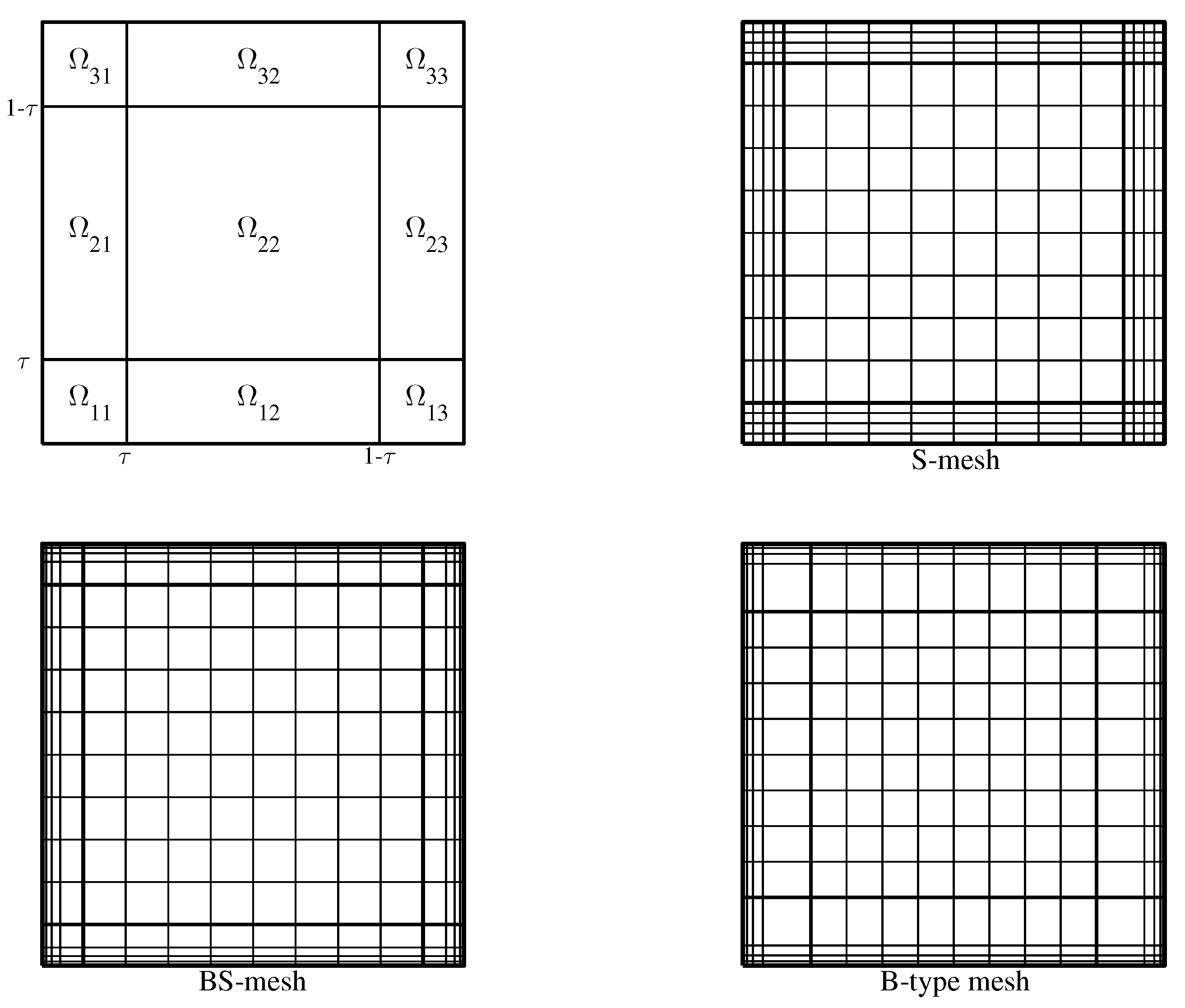
3. Layer-Adapted Meshes

To introduce the layer-adapted meshes, we extract some precise information from the exact solution of (1) and its derivatives in [21] (Theorem 2.2) and in [26] (Theorem 4.2).

Proposition 1.

Assume that the solution u of (1) can be decomposed by

$$u=S+\sum _{k=1}^4{W}_k+\sum _{k=1}^4{Z}_k,(x,y)\in \overline{\mathsf{\Omega }},$$

(9)

where S is a smooth part, $W_k$ is a boundary layer part and $Z_k$ is a corner layer part. More precisely, for $0\le i,j\le k+2$, there exists a constant C independent of ε such that

$$\begin{array}{c}\hfill \left|{\partial }_x^i{\partial }_y^{j}S\right|\le C,\left|{\partial }_x^i{\partial }_y^j{W}_1\right|\le C{\epsilon }^{-\frac{i}{2}}{e}^{-\frac{\beta x}{\sqrt{\epsilon }}},\left|{\partial }_x^i{\partial }_y^j{Z}_1\right|\le C{\epsilon }^{-\frac{i+j}{2}}{e}^{-\frac{\beta (x+y)}{\sqrt{\epsilon }}},\end{array}$$

(10)

and so on for the remaining terms. Here, ${\partial }_x^i{\partial }_y^{j}v=\frac{{\partial }^{i+j}v}{\partial x^i\partial y^j}$.

The layer-adapted mesh is constructed as follows: For notational simplification, we assume that $N_x=N_y=N$. Let $N\ge 4$ be a multiple of four. We introduce the mesh points

$$0=x_0<x_1<\dots <x_{N-1}<x_N=1,0=y_0<y_1<\dots <y_{N-1}<y_N=1,$$

and consider a tensor-product mesh with mesh points $(x_i,y_j)$. Because both meshes have the same structure, we only describe the mesh in the x-direction.

Suppose $\phi$ is a function defined in $[0,1/4]$ with

$$\begin{array}{c}\hfill \phi (0)=0,{\phi }^{\prime }>0,{\phi }^{″}\ge 0.\end{array}$$

(11)

We define the transition parameter

$$\tau =min\left\{\frac{1}{4},\frac{\sigma \sqrt{\epsilon }}{\beta }\phi (1/4)\right\},$$

(12)

where $\sigma >0$ is determined later. Assume that $\sqrt{\epsilon }\le N^{-1}$ means that we are in the singularly perturbed case. Moreover, $\epsilon$ is sufficiently small that (12) is replaced by $\tau =\frac{\sigma \sqrt{\epsilon }}{\beta }\phi (1/4)$.

The mesh in the x-direction is equidistant on $[\tau ,1-\tau ]$ with $N/2$ elements, but it is gradually divided on $[0,\tau ]$ and $[1-\tau ,1]$ with $N/4$ elements. Therefore, we set the mesh points as

$$x_i=\left\{\begin{array}{cc}\frac{\sigma \sqrt{\epsilon }}{\beta }\phi (i/N),\hfill & \mathrm{for}i=0,1,\dots ,N/4,\hfill \\ \tau +2(1-2\tau )(i/N-1/4),\hfill & \mathrm{for}i=N/4+1,\dots ,3N/4-1,\hfill \\ 1-\frac{\sigma \sqrt{\epsilon }}{\beta }\phi (1-i/N),\hfill & \mathrm{for}i=3N/4,\dots ,N.\hfill \end{array}\right.$$

(13)

In Table 1, we list three typical layer-adapted meshes [2] (Sections 1.2 and 1.3): Shishkin (S-mesh), Bakhvalov–Shishkin (BS mesh) and Bakhvalov-type (B-type mesh), together with $\psi =e^{-\phi }$ and the important quantity $max|{\psi }^{\prime }|$, which arises in error estimates. Figure 1 illustrates the divisions of $\mathsf{\Omega }$ and the generated meshes for $\epsilon ={10}^{-2}$ and $N=16$.

Table 1. Layer-adapted meshes.

	S-Mesh	BS-Mesh	B-Type Mesh
$\phi (t)$	$4tlnN$	$-ln\left[1-4(1-N^{-1})t\right]$	$-ln\left[1-4(1-\sqrt{\epsilon })t\right]$
$\psi (t)$	$N^{-4t}$	$1-4(1-N^{-1})t$	$1-4(1-\sqrt{\epsilon })t$
$max|{\psi }^{\prime }|$	$ClnN$	C	C

Figure 1. The division of $\mathsf{\Omega }$ and three types of layer-adapted meshes.

Note that for these meshes and under the assumption $\sqrt{\epsilon }\le N^{-1}$, we always have $\tau \ge \frac{\sigma \sqrt{\epsilon }}{\beta }lnN$.

In the following, we state two preliminary lemmas that will be frequently employed in the subsequent analysis. Because $h_{x,i}=h_{y,i}$, $i=1,2,\dots ,N$, we simply use $h_i$ to denote one of them.

Lemma 1.

Suppose that

$${\mathsf{\Theta }}_i=min\left\{\frac{h_i}{\sqrt{\epsilon }},1\right\}{e}^{-\frac{\beta x_{i-1}}{\sigma \sqrt{\epsilon }}},i=1,2,\dots ,N/4.$$

Then, there exists a constant $C>0$ independent of ε and N such that

$$\begin{array}{cc}\hfill \underset{1\le i\le N/4}{max}{\mathsf{\Theta }}_i\le & C{N}^{-1}max\left|{\psi }^{\prime }\right|,\hfill \end{array}$$

(14a)

$$\begin{array}{cc}\hfill \sum _{i=1}^{N/4}{\mathsf{\Theta }}_i\le & C.\hfill \end{array}$$

(14b)

Because of the symmetry of the mesh and layer function, (14) is also valid for the cases with $y_i$, $1-y_{i-1}$ and $1-x_{i-1}$.

Proof. 

See in [9] (Lemma 3.1) for details. □

Lemma 2.

We have $h_{N/4+1}=h_{N/4+2}=\dots =h_{3N/4}$ and $\hslash \ge C\sqrt{\epsilon }{N}^{-1}max\left|{\psi }^{\prime }\right|$. For the S-type meshes,

$$\begin{array}{c}\hfill \left\{\begin{array}{cc}1\ge h_i/h_{i+1}\ge C\hfill & i=1,2,\dots ,N/4-1,\hfill \\ 1\ge h_{i+1}/h_i\ge C\hfill & i=3N/4+1,3N/4+2,\dots ,N-1.\hfill \end{array}\right.\end{array}$$

(15)

For the B-type mesh,

$$\begin{array}{c}\hfill \left\{\begin{array}{cc}1\ge h_i/h_{i+1}\ge C\hfill & i=1,2,\dots ,N/4-2,\hfill \\ 1\ge h_{i+1}/h_i\ge C\hfill & i=3N/4+2,3N/4+3,\dots ,N-1.\hfill \end{array}\right.\end{array}$$

(16)

Moreover,

$$h_{ly}\equiv \underset{\begin{array}{c}i=1,\dots ,N/4\\ i=3N/4,\dots ,N\end{array}}{max}{h}_i\le C\varrho \equiv C\left\{\begin{array}{cc}\sqrt{\epsilon },\hfill & forS-type meshes,\hfill \\ N^{-1},\hfill & fora B-type meshes.\hfill \end{array}\right.$$

(17)

Proof. 

It can be seen that $h_{N/4+1}=h_{N/4+2}=\dots =h_{3N/4}$. (15) and (16) can be verified trivially (see [9] (Lemma 3.2)). By (13) and (11), and $\psi =e^{-\phi }$, we have

$$\begin{array}{cc}\hfill \hslash \ge & C\sqrt{\epsilon }{N}^{-1}min|{\phi }^{\prime }|=C\sqrt{\epsilon }{N}^{-1}|{\phi }^{\prime }(0)|=C\sqrt{\epsilon }{N}^{-1}|{\psi }^{\prime }(0)|=C\sqrt{\epsilon }{N}^{-1}max\left|{\psi }^{\prime }\right|.\hfill \end{array}$$

Now, we prove (17). Combining the fact that $h_{ly}\le C{N}^{-1}$ with the inequality

$$\begin{array}{c}\hfill h_{ly}\le C\sqrt{\epsilon }{N}^{-1}max|{\phi }^{\prime }|\le C\sqrt{\epsilon }{N}^{-1}\left|{\phi }^{\prime }(1/4)\right|,\end{array}$$

we obtain

$$\begin{array}{c}\hfill h_{ly}\le Cmin\left\{\sqrt{\epsilon }{N}^{-1}\left|{\phi }^{\prime }(1/4)\right|,N^{-1}\right\},\end{array}$$

(18)

which implies (17). □

4. Convergence Analysis

In this section, we perform uniform convergence analysis for the LDG method on layer-adapted meshes. Two related norms are considered.

The first is the energy norm, which is naturally derived from the formulation of the LDG method; that is, $⫴\mathsf{𝕨}{⫴}_E^2\equiv B(\mathsf{𝕨};\mathsf{𝕨})$. Therefore, we obtain

$$\begin{array}{cc}\hfill ⫴\mathsf{𝕨}{⫴}_E^2=& {\epsilon }^{-1}{∥\mathsf{𝕡}∥}^2+{\epsilon }^{-1}{∥\mathsf{𝕢}∥}^2+{∥b^{1/2}\mathsf{𝕦}∥}^2\hfill \\ \hfill & +\sum _{j=1}^N\sum _{i=0}^N{⟨{\lambda }_{i,y},{\left[\left[\mathsf{𝕦}\right]\right]}_{i,y}^2⟩}_{J_j}+\sum _{i=1}^N\sum _{j=0}^N{⟨{\lambda }_{x,j},{\left[\left[\mathsf{𝕦}\right]\right]}_{x,j}^2⟩}_{I_i},\hfill \end{array}$$

(19)

by using integration by parts and some trivial manipulations. Here,

${∥z∥}^2={\sum }_{K\in {\mathsf{\Omega }}_N}{∥z∥}_K^2$ and ${∥z∥}_K^2={⟨z,z⟩}_K$.

However, this norm is inadequate for reaction–diffusion problems because the layer contributions are not “seen” In fact, letting $u=e^{-\beta (x+y)/\sqrt{\epsilon }}$, we have $⫴(u,\epsilon u_x,\epsilon u_y){⫴}_E=\mathcal{O}(\sqrt[4]{\epsilon })$, which vanishes as $\epsilon \to 0$. Thus, the following “balanced” norm is introduced:

$$\begin{array}{cc}\hfill ⫴\mathsf{𝕨}{⫴}_B^2=& {\epsilon }^{-3/2}{∥\mathsf{𝕡}∥}^2+{\epsilon }^{-3/2}{∥\mathsf{𝕢}∥}^2+{∥b^{1/2}\mathsf{𝕦}∥}^2\hfill \\ \hfill & +\sum _{j=1}^N\sum _{i=0}^N{⟨1,{\left[\left[\mathsf{𝕦}\right]\right]}_{i,y}^2⟩}_{J_j}+\sum _{i=1}^N\sum _{j=0}^N{⟨1,{\left[\left[\mathsf{𝕦}\right]\right]}_{x,j}^2⟩}_{I_i}.\hfill \end{array}$$

(20)

This norm is balanced in the sense that both the regular and layer parts are bounded away from zero uniformly in $\epsilon$. We drop the penalty parameter $\lambda$ because they will be taken as $O(\sqrt{\epsilon })$ in the subsequent analysis and computation of balanced-norm error.

In the following subsections, we perform convergence analysis for these two norms. Different projections are introduced, and the related approximation properties are investigated.

4.1. Convergence of Balanced Norm

First, we analyse the LDG method for the balanced norm (20). Let $\omega \in C^1({\mathsf{\Omega }}_N)$ and $\omega \ge {\omega }_0>0$ be a general weight function. We define the piecewise local weight $L^2$ projection ${\mathsf{\Pi }}_{\omega }$ as follows: For each element $K\in {\mathsf{\Omega }}_N$ and for any $z\in L^2({\mathsf{\Omega }}_N)$, ${\mathsf{\Pi }}_{\omega }z\in V_N$ satisfies

$$\begin{array}{c}\hfill {⟨\omega {\mathsf{\Pi }}_{\omega }z,\mathsf{𝕧}⟩}_K={⟨\omega z,\mathsf{𝕧}⟩}_K,\forall \mathsf{𝕧}\in {\mathcal{Q}}^k(K).\end{array}$$

(21)

In the special case of $\omega =1$, this operator reduces to the classical local $L^2$ projection, which is denoted by $\mathsf{\Pi }$.

Lemma 3.

[27] (Lemma 2.14) There exists a constant $C>0$, independent of the element size and z, such that

$$\begin{array}{cc}\hfill {∥{\mathsf{\Pi }}_{\omega }z∥}_{L^m(K_{ij})}\le & C{∥z∥}_{L^m(K_{ij})},\hfill \end{array}$$

(22a)

$$\begin{array}{cc}\hfill {∥z-{\mathsf{\Pi }}_{\omega }z∥}_{L^m(K_{ij})}\le & C\left[h_i^{k+1}{∥{\partial }_x^{k+1}z∥}_{L^m(K_{ij})}+h_j^{k+1}{∥{\partial }_y^{k+1}z∥}_{L^m(K_{ij})}\right],\hfill \end{array}$$

(22b)

where $m\in \{2,\infty \}$.

Lemma 4.

Let $\sigma \ge k+1.5$. Then, there holds

$$\begin{array}{cc}\hfill ∥u-{\mathsf{\Pi }}_{\omega }u∥& \le C\left[\sqrt[4]{\epsilon }(N^{-1}max|{\psi }^{\prime }{|)}^{k+1}+N^{-(k+1)}\right],\hfill \end{array}$$

(23a)

$$\begin{array}{cc}\hfill {∥u-{\mathsf{\Pi }}_{\omega }u∥}_{L^{\infty }({\mathsf{\Omega }}_N)}& \le C(N^{-1}max|{\psi }^{\prime }{|)}^{k+1},\hfill \end{array}$$

(23b)

$$\begin{array}{cc}\hfill \sum _{j=1}^N\sum _{i=1}^{N-1}{∥{(u-{\mathsf{\Pi }}_{\omega }u)}_{i,y}^{-}∥}_{J_j}^2& \le C(N^{-1}max|{\psi }^{\prime }{|)}^{2k+1},\hfill \end{array}$$

(23c)

$$\begin{array}{cc}\hfill \sum _{j=1}^N\sum _{i=0}^N{⟨1,{\left[[u-{\mathsf{\Pi }}_{\omega }u]\right]}_{i,y}^2⟩}_{J_j}& \le C(N^{-1}max|{\psi }^{\prime }{|)}^{2k+1},\hfill \end{array}$$

(23d)

$$\begin{array}{cc}\hfill ∥p-{\mathsf{\Pi }}_{\omega }p∥& \le C{\epsilon }^{\frac{3}{4}}(N^{-1}max|{\psi }^{\prime }{|)}^{k+1},\hfill \end{array}$$

(23e)

$$\begin{array}{cc}\hfill \sum _{j=1}^N{∥{(p-{\mathsf{\Pi }}_{\omega }p)}_{N,y}^{-}∥}_{J_j}^2& \le C\epsilon (N^{-1}max|{\psi }^{\prime }{|)}^{2(k+1)},\hfill \end{array}$$

(23f)

$$\begin{array}{cc}\hfill \sum _{j=1}^N\sum _{i=0}^{N-1}{∥{(p-{\mathsf{\Pi }}_{\omega }p)}_{i,y}^{+}∥}_{J_j}^2& \le C\epsilon (N^{-1}max|{\psi }^{\prime }{|)}^{2k+1},\hfill \end{array}$$

(23g)

where $C>0$ is independent of ε and N. A similar procedure applies for u and q in other spatial directions.

Proof. 

The proof is provided in the Appendix A.1. □

Theorem 1.

Suppose that ${\lambda }_{i,y}={\lambda }_{x,j}=\sqrt{\epsilon }$ for $i,j=0,1,\dots ,N$. Let $\mathit{w}=(u,p,q)$ be the solution to problem (1), satisfying Proposition 1; furthermore, let $\mathsf{𝕨}=(\mathsf{𝕦},\mathsf{𝕡},\mathsf{𝕢})\in {\mathcal{V}}_N^3$ be the numerical solution of the LDG scheme (5) on layer-adapted meshes (13) when $\sigma \ge k+1.5$. Here, $k\ge 0$ is the degree of the piecewise polynomials used in the discontinuous finite element space. Then, there exists a constant $C>0$, independent of ε and N, such that

$$\begin{array}{c}\hfill ⫴\mathit{w}-\mathsf{𝕨}{⫴}_B\le C{N}^{-k}(max|{\psi }^{\prime }{|)}^{k+1/2}.\end{array}$$

(24)

Proof. 

Denote $\mathit{e}=\mathit{w}-\mathsf{𝕨}=\mathit{\eta }-\mathit{\xi }$ as

$$\begin{array}{cc}\hfill \mathit{\eta }& =({\eta }_u,{\eta }_p,{\eta }_q)=(u-{\mathsf{\Pi }}_{b}u,p-\mathsf{\Pi }p,q-\mathsf{\Pi }q),\hfill \end{array}$$

(25a)

$$\begin{array}{cc}\hfill \mathit{\xi }& =({\xi }_u,{\xi }_p,{\xi }_q)=(\mathsf{𝕦}-{\mathsf{\Pi }}_{b}u,\mathsf{𝕡}-\mathsf{\Pi }p,\mathsf{𝕢}-\mathsf{\Pi }q)\in {\mathcal{V}}_N^3,\hfill \end{array}$$

(25b)

where ${\mathsf{\Pi }}_b$ is defined in (21) with weight $\omega =b$.

From Proposition 1 and the consistency of numerical flux, we obtain the error equation:

$$\begin{array}{cc}\hfill B(\mathit{\xi };\mathsf{𝕫})& =B(\mathit{\eta };\mathsf{𝕫})\hfill \\ & ={\mathcal{T}}_1(\mathit{\eta };\mathsf{𝕫})+{\mathcal{T}}_2({\eta }_u;\mathsf{𝕫})+{\mathcal{T}}_3(\mathit{\eta };\mathsf{𝕧})+{\mathcal{T}}_4({\eta }_u;\mathsf{𝕧}).\hfill \end{array}$$

(26)

It can be seen that ${\mathcal{T}}_1(\mathit{\eta };\mathsf{𝕫})=0$.

To bound ${\mathcal{T}}_2({\eta }_u;\mathsf{𝕫})$, we use the Cauchy–Schwarz inequality, inverse inequality, $C\sqrt{\epsilon }{N}^{-1}$$max|{\psi }^{\prime }|\le \hslash \le C{N}^{-1}$, (23b), and ${\epsilon }^{-1/2}∥\mathsf{𝕤}∥\le ⫴\mathsf{𝕫}{⫴}_E$ to obtain

$$\begin{array}{cc}\hfill |⟨{\eta }_u,{\mathsf{𝕤}}_x⟩|\le & \sum _K{∥{\eta }_u∥}_K{∥{\mathsf{𝕤}}_x∥}_K\le C\sum _K{\left|K\right|}^{1/2}{∥{\eta }_u∥}_{L^{\infty }(K)}{h}_x^{-1}{∥\mathsf{𝕤}∥}_K\hfill \\ \hfill \le & C{\left(\sum _K\frac{h_y}{h_x}{∥{\eta }_u∥}_{L^{\infty }(K)}^2\right)}^{1/2}∥\mathsf{𝕤}∥\le C\sqrt[4]{\epsilon }{N}^{-k}(max|{\psi }^{\prime }{|)}^{k+1/2}⫴\mathsf{𝕫}{⫴}_E,\hfill \end{array}$$

and we use (23c) to obtain

$$\begin{array}{cc}\hfill \left|\sum _{j=1}^N\sum _{i=1}^{N-1}{⟨{({\eta }_u)}_{i,y}^{-},{\left[\left[\mathsf{𝕤}\right]\right]}_{i,y}⟩}_{J_j}\right|\le & C{\left(\sum _{j=1}^N\sum _{i=1}^{N-1}{∥{({\eta }_u)}_{i,y}^{-}∥}_{J_j}^2\right)}^{1/2}({\hslash }^{-1/2}∥\mathsf{𝕤}∥)\hfill \\ \hfill \le & C\sqrt[4]{\epsilon }(N^{-1}max|{\psi }^{\prime }{|)}^k⫴\mathsf{𝕫}{⫴}_E.\hfill \end{array}$$

Consequently, we have

$$\begin{array}{cc}\hfill {\mathcal{T}}_2({\eta }_u;\mathsf{𝕫})\le & C\sqrt[4]{\epsilon }{N}^{-k}(max|{\psi }^{\prime }{|)}^{k+1/2}⫴\mathsf{𝕫}{⫴}_E.\hfill \end{array}$$

(27)

Analogously, we have

$$\begin{array}{cc}\hfill {\mathcal{T}}_3(\mathit{\eta };\mathsf{𝕧})& =\sum _{j=1}^N\left[\sum _{i=0}^{N-1}{⟨{({\eta }_p)}_{i,y}^{+},{\left[\left[\mathsf{𝕧}\right]\right]}_{i,y}^{-}⟩}_{J_j}-{⟨{({\eta }_p)}_{N,y}^{-},{\mathsf{𝕧}}_{N,y}^{-}⟩}_{J_j}\right]\hfill \\ \hfill & +\sum _{i=1}^N\left[\sum _{j=0}^{N-1}{⟨{({\eta }_q)}_{x,j}^{+},{\left[\left[\mathsf{𝕧}\right]\right]}_{x,j}^{-}⟩}_{I_i}-{⟨{({\eta }_q)}_{x,N}^{-},{\mathsf{𝕧}}_{x,N}^{-}⟩}_{I_i}\right]\hfill \\ \hfill & \le C{\left(\sum _{j=1}^N\sum _{i=0}^{N-1}{\epsilon }^{-1}{∥{({\eta }_p)}_{i,y}^{+}∥}_{J_j}^2+\sum _{j=1}^N{\epsilon }^{-1}{∥{({\eta }_p)}_{N,y}^{-}∥}_{J_j}^2\right)}^{1/2}(\sqrt{\epsilon }{\hslash }^{-1/2}∥\mathsf{𝕧}∥)\hfill \\ \hfill & +C{\left(\sum _{i=1}^N\sum _{j=0}^{N-1}{\epsilon }^{-1}{∥{({\eta }_q)}_{x,j}^{+}∥}_{I_i}^2+\sum _{i=1}^N{\epsilon }^{-1}{∥{({\eta }_q)}_{x,N}^{-}∥}_{I_i}^2\right)}^{1/2}(\sqrt{\epsilon }{\hslash }^{-1/2}∥\mathsf{𝕧}∥)\hfill \\ \hfill & \le C{\hslash }^{-1/2}\sqrt{\epsilon }(N^{-1}max|{\psi }^{\prime }{|)}^{k+1/2}∥\mathsf{𝕧}∥\hfill \\ \hfill & \le C\sqrt[4]{\epsilon }(N^{-1}max|{\psi }^{\prime }{|)}^k⫴\mathsf{𝕫}{⫴}_E.\hfill \end{array}$$

(28)

Here, (23f) and (23g) are used.

Finally, we use the Cauchy–Schwarz inequality, (23d), and the assumption that ${\lambda }_{i,y}={\lambda }_{x,j}=\sqrt{\epsilon }$ for $i,j=0,1,\dots ,N$, to obtain

$$\begin{array}{cc}\hfill {\mathcal{T}}_4({\eta }_u;\mathsf{𝕧})& =\sum _{j=1}^N\sum _{i=0}^N{⟨{\lambda }_{i,y}{\left[\left[{\eta }_u\right]\right]}_{i,y},{\left[\left[\mathsf{𝕧}\right]\right]}_{i,y}⟩}_{J_j}+\sum _{i=1}^N\sum _{j=0}^N{⟨{\lambda }_{x,j}{\left[\left[{\eta }_u\right]\right]}_{x,j},{\left[\left[\mathsf{𝕧}\right]\right]}_{x,j}⟩}_{I_i}\hfill \\ & \le {\left[\sum _{i=0}^N\sum _{j=1}^N{\lambda }_{i,y}{⟨1,{\left[\left[{\eta }_u\right]\right]}_{i,y}^2⟩}_{J_j}+\sum _{j=0}^N\sum _{i=1}^N{\lambda }_{x,j}{⟨1,{\left[\left[{\eta }_u\right]\right]}_{x,j}^2⟩}_{I_i}\right]}^{1/2}⫴\mathsf{𝕫}{⫴}_E\hfill \\ & \le C\sqrt[4]{\epsilon }(N^{-1}max|{\psi }^{\prime }{|)}^{k+1/2}⫴\mathsf{𝕫}{⫴}_E.\hfill \end{array}$$

(29)

From (27)–(29), we have

$$\begin{array}{c}\hfill ⫴\mathit{\xi }{⫴}_E^2=B(\mathit{\xi };\mathit{\xi })=B(\mathit{\eta };\mathit{\xi })\le C\sqrt[4]{\epsilon }{N}^{-k}(max|{\psi }^{\prime }{|)}^{k+1/2}⫴\mathit{\xi }{⫴}_E,\end{array}$$

(30)

which implies

$$\begin{array}{c}\hfill ⫴\mathit{\xi }{⫴}_B\le {\epsilon }^{-1/4}⫴\mathit{\xi }{⫴}_E\le C{N}^{-k}(max|{\psi }^{\prime }{|)}^{k+1/2},\end{array}$$

(31)

from the definitions (19) and (20) and the choice of ${\lambda }_{i,y}={\lambda }_{x,j}=\sqrt{\epsilon }$ ($i,j=0,1,\dots ,N$). Using (23) and a trivial inequality, we derive (24). □

Remark that for the meshes listed in Table 1, one has balanced-norm error estimate

$$⫴\mathit{w}-\mathsf{𝕨}{⫴}_B\le \left\{\begin{array}{cc}C{N}^{-k}{(lnN)}^{k+1/2},\hfill & \mathrm{for} \mathrm{S}-\mathrm{mesh},\hfill \\ C{N}^{-k},\hfill & \mathrm{for} \mathrm{BS}-,\mathrm{B}-\mathrm{type} \mathrm{mesh}.\hfill \end{array}\right.$$

(32)

4.2. Improvement of Convergence in Energy Norm

By the analysis in Theorem 1, one can only obtain the energy-error bound of order $O(\sqrt[4]{\epsilon }{N}^{-k}(max|{\psi }^{\prime }{|)}^{k+1/2})$. In this subsection, we perform an elaborate analysis and establish a more sharp convergence result in the energy norm. The following local Gauss–Radau projections are required.

For each element $K_{ij}\in {\mathsf{\Omega }}_N$ and for any $z\in H^1(K_{ij})$, ${\mathsf{\Pi }}^{-}z,{\mathsf{\Pi }}_x^{+}z,{\mathsf{\Pi }}_y^{+}z\in {\mathcal{Q}}^k(K_{ij})$ are defined as

$$\begin{array}{cc}\hfill & \left\{\begin{array}{cc}{⟨{\mathsf{\Pi }}^{-}z,\mathsf{𝕧}⟩}_{K_{ij}}={⟨z,\mathsf{𝕧}⟩}_{K_{ij}},\hfill & \forall \mathsf{𝕧}\in {\mathcal{Q}}^{k-1}(K_{ij}),\hfill \\ {⟨{({\mathsf{\Pi }}^{-}z)}_{i,y}^{-},\mathsf{𝕧}⟩}_{J_j}={⟨z_{i,y}^{-},\mathsf{𝕧}⟩}_{J_j},\hfill & \forall \mathsf{𝕧}\in {\mathcal{P}}^{k-1}(J_j),\hfill \\ {⟨{({\mathsf{\Pi }}^{-}z)}_{x,j}^{-},\mathsf{𝕧}⟩}_{I_i}={⟨z_{x,j}^{-},\mathsf{𝕧}⟩}_{I_i},\hfill & \forall \mathsf{𝕧}\in {\mathcal{P}}^{k-1}(I_i),\hfill \\ ({\mathsf{\Pi }}^{-}z)(x_i^{-},y_j^{-})=z(x_i^{-},y_j^{-}).\hfill \end{array}\right.\hfill \end{array}$$

(33a)

$$\begin{array}{cc}\hfill & \left\{\begin{array}{cc}{⟨{\mathsf{\Pi }}_x^{+}z,\mathsf{𝕧}⟩}_{K_{ij}}={⟨z,\mathsf{𝕧}⟩}_{K_{ij}},\hfill & \forall \mathsf{𝕧}\in {\mathcal{P}}^{k-1}(I_i)\otimes {\mathcal{P}}^k(J_j),\hfill \\ {⟨{({\mathsf{\Pi }}_x^{+}z)}_{i,y}^{+},\mathsf{𝕧}⟩}_{J_j}={⟨z_{i,y}^{+},\mathsf{𝕧}⟩}_{J_j},\hfill & \forall \mathsf{𝕧}\in {\mathcal{P}}^k(J_j).\hfill \end{array}\right.\hfill \end{array}$$

(33b)

$$\begin{array}{cc}\hfill & \left\{\begin{array}{cc}{⟨{\mathsf{\Pi }}_y^{+}z,\mathsf{𝕧}⟩}_{K_{ij}}={⟨z,\mathsf{𝕧}⟩}_{K_{ij}}\hfill & \forall \mathsf{𝕧}\in {\mathcal{P}}^k(I_i)\otimes {\mathcal{P}}^{k-1}(J_j),\hfill \\ {⟨{({\mathsf{\Pi }}_y^{+}z)}_{x,j}^{+},\mathsf{𝕧}⟩}_{J_j}={⟨z_{x,j}^{+},\mathsf{𝕧}⟩}_{J_j},\hfill & \forall \mathsf{𝕧}\in {\mathcal{P}}^k(I_i).\hfill \end{array}\right.\hfill \end{array}$$

(33c)

Lemma 5.

[9] (Inequality (4.4)) There exists a constant $C>0$, independent of the element size and z, such that

$$\begin{array}{cc}\hfill {∥{\mathsf{\Pi }}^{-}z∥}_{K_{ij}}\le & C\left[{∥z∥}_{K_{ij}}+h_j^{1/2}{∥z_{x,j}^{-}∥}_{I_i}+h_i^{1/2}{∥z_{i,y}^{-}∥}_{J_j}+h_i^{1/2}{h}_j^{1/2}\left|z_{i,j}^{-}\right|\right],\hfill \end{array}$$

(34a)

$$\begin{array}{cc}\hfill {∥{\mathsf{\Pi }}_x^{+}z∥}_{K_{ij}}\le & C\left[{∥z∥}_{K_{ij}}+h_i^{1/2}{∥z_{i-1,y}^{+}∥}_{J_j}\right],\hfill \end{array}$$

(34b)

$$\begin{array}{cc}\hfill {∥{\mathsf{\Pi }}_y^{+}z∥}_{K_{ij}}\le & C\left[{∥z∥}_{K_{ij}}+h_j^{1/2}{∥z_{x,j-1}^{+}∥}_{I_i}\right],\hfill \end{array}$$

(34c)

$$\begin{array}{cc}\hfill {∥\mathsf{\Phi }z∥}_{L^{\infty }(K_{ij})}\le & C{∥z∥}_{L^{\infty }(K_{ij})},\hfill \end{array}$$

(34d)

$$\begin{array}{cc}\hfill {∥z-\mathsf{\Phi }z∥}_{L^m(K_{ij})}\le & C\left[h_i^{k+1}{∥{\partial }_x^{k+1}z∥}_{L^m(K_{ij})}+h_j^{k+1}{∥{\partial }_y^{k+1}z∥}_{L^m(K_{ij})}\right],\hfill \end{array}$$

(34e)

where $\mathsf{\Phi }\in \{{\mathsf{\Pi }}^{-},{\mathsf{\Pi }}_x^{+},{\mathsf{\Pi }}_y^{+}\}$, $m\in \{2,\infty \}$ and $z_{i,j}^{-}=z(x_i^{-},y_j^{-})$.

Lemma 6.

Let $\sigma \ge k+1.5$. Then, there exists a constant $C>0$ independent of ε and N such that

$$\begin{array}{cc}\hfill ∥u-{\mathsf{\Pi }}^{-}u∥& \le C\left[(\sqrt[4]{\epsilon }+\sqrt{\varrho })(N^{-1}max|{\psi }^{\prime }{|)}^{k+1}+N^{-(k+1)}\right],\hfill \end{array}$$

(35a)

$$\begin{array}{cc}\hfill \sum _{j=1}^N{∥{(u-{\mathsf{\Pi }}^{-}u)}_{N,y}^{-}∥}_{J_j}^2& \le C\left[(\sqrt{\epsilon }+\varrho )(N^{-1}max|{\psi }^{\prime }{|)}^{2(k+1)}+N^{-2(k+1)}\right],\hfill \end{array}$$

(35b)

$$\begin{array}{cc}\hfill {\epsilon }^{-\frac{1}{2}}∥p-{\mathsf{\Pi }}_x^{+}p∥& \le C[(\sqrt[4]{\epsilon }+\sqrt{\varrho })(N^{-1}max|{\psi }^{\prime }{|)}^{k+1}+N^{-(k+1)}],\hfill \end{array}$$

(35c)

$$\begin{array}{cc}\hfill \sum _{j=1}^N{\epsilon }^{-1}{∥{(p-{\mathsf{\Pi }}_x^{+}p)}_{N,y}^{-}∥}_{J_j}^2& \le C(N^{-1}max|{\psi }^{\prime }{|)}^{2(k+1)},\hfill \end{array}$$

(35d)

where ϱ is given by (17). Similarly, we can obtain the same conclusions in another spatial direction.

Proof. 

The proof is provided in the Appendix A.2. □

Theorem 2.

Suppose that ${\lambda }_{i,y}={\lambda }_{x,j}=0$ for $i,j=0,1,\dots ,N-1$, ${\lambda }_{N,y}={\lambda }_{x,N}=\sqrt{\epsilon }$. Let $\mathit{w}=(u,p,q)$ be the solution to problem (1), which satisfies Proposition 1; furthermore, let $\mathsf{𝕨}=(\mathsf{𝕦},\mathsf{𝕡},\mathsf{𝕢})\in {\mathcal{V}}_N^3$ be the numerical solution of the LDG scheme (5) on layer-adapted meshes (13) with $\sigma \ge k+2$. Here, $k\ge 0$ is the degree of the piecewise polynomials used in the discontinuous finite element space. Then, there exists a constant $C>0$ independent of ε and N such that

$$⫴\mathit{w}-\mathsf{𝕨}{⫴}_E\le \left\{\begin{array}{cc}C\left[\sqrt[4]{\epsilon }{(N^{-1}lnN)}^{k+1}+N^{-(k+1)}\right],\hfill & for\mathrm{S}-mesh,\hfill \\ C{N}^{-(k+1)},\hfill & for \mathrm{for}BS-,\mathrm{B}-type mesh.\hfill \end{array}\right.$$

(36)

Proof. 

We follow the proof of Theorem 1. Instead of the projection $({\mathsf{\Pi }}_b,\mathsf{\Pi },\mathsf{\Pi })$ for $u,p$ and q, we use $({\mathsf{\Pi }}^{-},{\mathsf{\Pi }}_x^{+},{\mathsf{\Pi }}_y^{+})$ in (25).

Using the Cauchy–Schwarz inequality, (35a) and (35c), we obtain

$$\begin{array}{cc}\hfill {\mathcal{T}}_1(\mathit{\eta };\mathsf{𝕫})\le & C\left({\epsilon }^{-1/2}∥{\eta }_p∥+{\epsilon }^{-1/2}∥{\eta }_q∥+{∥b^{1/2}∥}_{L^{\infty }({\mathsf{\Omega }}_N)}∥{\eta }_u∥\right)⫴\mathsf{𝕫}{⫴}_E\hfill \\ \hfill \le & C\left[(\sqrt[4]{\epsilon }+\sqrt{\varrho })(N^{-1}max|{\psi }^{\prime }{|)}^{k+1}+N^{-(k+1)}\right]⫴\mathsf{𝕫}{⫴}_E.\hfill \end{array}$$

(37)

From (33b), (33c) and (35d), ${\lambda }_{N,y}={\lambda }_{x,N}=\sqrt{\epsilon }$, and the Cauchy–Schwarz inequality, we obtain

$$\begin{array}{cc}\hfill {\mathcal{T}}_3(\mathit{\eta };\mathsf{𝕧})=& -\sum _{j=1}^N{⟨{({\eta }_p)}_{N,y}^{-},{\mathsf{𝕧}}_{N,y}^{-}⟩}_{J_j}-\sum _{i=1}^N{⟨{({\eta }_q)}_{x,N}^{-},{\mathsf{𝕧}}_{x,N}^{-}⟩}_{I_i}\hfill \\ \hfill \le & {\left[\sum _{j=1}^N\frac{1}{{\lambda }_{N,y}}{∥{({\eta }_p)}_{N,y}^{-}∥}_{J_j}^2+\sum _{i=1}^N\frac{1}{{\lambda }_{x,N}}{∥{({\eta }_q)}_{x,N}^{-}∥}_{I_i}^2\right]}^{1/2}⫴\mathsf{𝕫}{⫴}_E\hfill \\ \hfill \le & C\sqrt[4]{\epsilon }(N^{-1}max|{\psi }^{\prime }{|)}^{k+1}⫴\mathsf{𝕫}{⫴}_E.\hfill \end{array}$$

(38)

Similarly, we have

$$\begin{array}{cc}\hfill {\mathcal{T}}_4({\eta }_u;\mathsf{𝕧})& =\sum _{j=1}^N{⟨{\lambda }_{N,y}{({\eta }_u)}_{N,y}^{-},{\mathsf{𝕧}}_{N,y}^{-}⟩}_{J_j}+\sum _{i=1}^N{⟨{\lambda }_{x,N}{({\eta }_u)}_{x,N}^{-},{\mathsf{𝕧}}_{x,N}^{-}⟩}_{I_i}\hfill \\ & \le {\left[\sum _{j=1}^N{\lambda }_{N,y}{∥{({\eta }_u)}_{N,y}^{-}∥}_{J_j}^2+\sum _{i=1}^N{\lambda }_{x,N}{∥{({\eta }_u)}_{x,N}^{-}∥}_{I_i}^2\right]}^{1/2}⫴\mathsf{𝕫}{⫴}_E\hfill \\ & \le C\sqrt[4]{\epsilon }\left[(\sqrt[4]{\epsilon }+\sqrt{\varrho })(N^{-1}max|{\psi }^{\prime }{|)}^{k+1}+N^{-(k+1)}\right]⫴\mathsf{𝕫}{⫴}_E,\hfill \end{array}$$

(39)

where (35b) is used.

To bound ${\mathcal{T}}_2({\eta }_u;\mathsf{𝕫})$, we follow [9] (Theorem 4.1) and investigate the ${\epsilon }^{1/4}$-factor in the upper-bound. On each element $K_{ij}$, we define the bilinear forms as

$$\begin{array}{cc}\hfill {\mathcal{A}}_{ij}^1({\eta }_u;v)=& {⟨{\eta }_u,v_x⟩}_{K_{ij}}-{⟨{({\eta }_u)}_{i,y}^{-},v_{i,y}^{-}⟩}_{J_j}+{⟨{({\eta }_u)}_{i-1,y}^{-},v_{i-1,y}^{+}⟩}_{J_j},\hfill \\ \hfill {\mathcal{A}}_{ij}^2({\eta }_u;v)=& {⟨{\eta }_u,v_y⟩}_{K_{ij}}-{⟨{({\eta }_u)}_{x,j}^{-},v_{x,j}^{-}⟩}_{I_i}+{⟨{({\eta }_u)}_{x,j-1}^{-},v_{x,j-1}^{+}⟩}_{I_i}.\hfill \end{array}$$

We have [9] (Inequality (4.15))

$$\begin{array}{cc}\hfill |{\mathcal{A}}_{ij}^1({\eta }_u;v)|\le & C\sqrt{\frac{h_j}{h_i}}\left[h_i^{k+2}{∥{\partial }_x^{k+2}u∥}_{L^{\infty }(K_{ij})}+h_j^{k+2}{∥{\partial }_y^{k+2}u∥}_{L^{\infty }(K_{ij})}\right]{∥v∥}_{K_{ij}},\hfill \end{array}$$

(40a)

$$\begin{array}{cc}\hfill |{\mathcal{A}}_{ij}^1({\eta }_u;v)|\le & C\sqrt{\frac{h_j}{h_i}}{∥u∥}_{L^{\infty }(K_{ij})}{∥v∥}_{K_{ij}}\hfill \end{array}$$

(40b)

for any $v\in {\mathcal{Q}}^k(K_{ij})$. Because $u=0$ on $\partial \mathsf{\Omega }$, we obtain

$$\begin{array}{cc}\hfill {\mathcal{T}}_2({\eta }_u;\mathsf{𝕫})& =\sum _{K_{ij}\in {\mathsf{\Omega }}_N}{\mathcal{A}}_{ij}^1({\eta }_u;\mathsf{𝕤})+\sum _{K_{ij}\in {\mathsf{\Omega }}_N}{\mathcal{A}}_{ij}^2({\eta }_u;\mathsf{𝕣}).\hfill \end{array}$$

By (40a), we have

$$\begin{array}{cc}\hfill & \sum _{K_{ij}\in {\mathsf{\Omega }}_N}{\mathcal{A}}_{ij}^1({\eta }_S;\mathsf{𝕤})\hfill \\ \hfill \le & C\sum _{K_{ij}\in {\mathsf{\Omega }}_N}\sqrt{\frac{h_j}{h_i}}\left[h_i^{k+2}{∥{\partial }_x^{k+2}S∥}_{L^{\infty }(K_{ij})}+h_j^{k+2}{∥{\partial }_y^{k+2}S∥}_{L^{\infty }(K_{ij})}\right]{∥\mathsf{𝕤}∥}_{K_{ij}}\hfill \\ \hfill \le & C{N}^{-(k+1)}{∥\mathsf{𝕤}∥}_{{\mathsf{\Omega }}_{22}}+C{\left[\sum _{K_{ij}\in {\mathsf{\Omega }}_N\backslash {\mathsf{\Omega }}_{22}}(\sqrt{\epsilon }max|{\psi }^{\prime }{|)}^{-1}{N}^{-2(k+2)}\right]}^{1/2}{∥\mathsf{𝕤}∥}_{\mathsf{\Omega }\backslash {\mathsf{\Omega }}_{22}}\hfill \\ \hfill \le & C\sqrt[4]{\epsilon }{N}^{-(k+1)}⫴\mathsf{𝕫}{⫴}_E,\hfill \end{array}$$

because $h_i\ge C\sqrt{\epsilon }{N}^{-1}max|{\psi }^{\prime }|\ge C\sqrt{\epsilon }{h}_{j}max\left|{\psi }^{\prime }\right|$ and ${\epsilon }^{-1/2}∥\mathsf{𝕤}∥\le ⫴\mathsf{𝕫}{⫴}_E$. Denote ${\mathsf{\Omega }}_{XL}={\mathsf{\Omega }}_{11}\cup {\mathsf{\Omega }}_{21}\cup {\mathsf{\Omega }}_{31}$, ${\mathsf{\Omega }}_{XM}={\mathsf{\Omega }}_{12}\cup {\mathsf{\Omega }}_{22}\cup {\mathsf{\Omega }}_{32}$, and ${\mathsf{\Omega }}_{XR}={\mathsf{\Omega }}_{13}\cup {\mathsf{\Omega }}_{23}\cup {\mathsf{\Omega }}_{33}$. Using (40a) and $\sigma \ge k+2$, we obtain

$$\begin{array}{cc}\hfill \sum _{K_{ij}\in {\mathsf{\Omega }}_{XM}\cup {\mathsf{\Omega }}_{XR}}{\mathcal{A}}_{ij}^1({\eta }_{W_1};\mathsf{𝕤})\le & C\sum _{K_{ij}\in {\mathsf{\Omega }}_{XM}\cup {\mathsf{\Omega }}_{XR}}\sqrt{\frac{h_j}{h_i}}{∥W_1∥}_{L^{\infty }(K_{ij})}{∥\mathsf{𝕤}∥}_{K_{ij}}\hfill \\ \hfill \le & C\sum _{K_{ij}\in {\mathsf{\Omega }}_{XM}\cup {\mathsf{\Omega }}_{XR}}{\epsilon }^{-1/4}{e}^{-\frac{\beta x_i}{\sqrt{\epsilon }}}{∥\mathsf{𝕤}∥}_{K_{ij}}\hfill \\ \hfill \le & C\sqrt[4]{\epsilon }{N}^{-(k+1)}⫴\mathsf{𝕫}{⫴}_E.\hfill \end{array}$$

Using (40), $\sigma \ge k+2$, and Lemma 1 yields

$$\begin{array}{cc}\hfill & \sum _{K_{ij}\in {\mathsf{\Omega }}_{XL}}{\mathcal{A}}_{ij}^1({\eta }_{W_1};\mathsf{𝕤})\hfill \\ \hfill \le & C\sum _{K_{ij}\in {\mathsf{\Omega }}_{XL}}\sqrt{\frac{h_j}{h_i}}min\left\{h_i^{k+2}{∥{\partial }_x^{k+2}{W}_1∥}_{L^{\infty }(K_{ij})}+h_j^{k+2}{∥{\partial }_y^{k+2}{W}_1∥}_{L^{\infty }(K_{ij})},{∥W_1∥}_{L^{\infty }(K_{ij})}\right\}{∥\mathsf{𝕤}∥}_{K_{ij}}\hfill \\ \hfill \le & C\sum _{K_{ij}\in {\mathsf{\Omega }}_{XL}}(\sqrt{\epsilon }max|{\psi }^{\prime }{|)}^{-1/2}{\mathsf{\Theta }}_i^{k+2}{∥\mathsf{𝕤}∥}_{K_{ij}}\hfill \\ \hfill \le & C\sqrt[4]{\epsilon }(max|{\psi }^{\prime }{|)}^{-1/2}{\left(\sum _{j=1}^N\sum _{i=1}^{N/4}{\mathsf{\Theta }}_i\right)}^{1/2}\left(\underset{1\le i\le N/4}{max}{\mathsf{\Theta }}_i^{k+3/2}\right)\left({\epsilon }^{-1/2}∥\mathsf{𝕤}∥\right)\hfill \\ \hfill \le & C\sqrt[4]{\epsilon }(N^{-1}max|{\psi }^{\prime }{|)}^{k+1}⫴\mathsf{𝕫}{⫴}_E.\hfill \end{array}$$

Analogously, we can bound ${\sum }_{K_{ij}\in {\mathsf{\Omega }}_N}{\mathcal{A}}_{ij}^1({\eta }_{\phi };\mathsf{𝕤})$ for $\phi =W_2,W_3,W_4,Z_1,Z_2,Z_3,Z_4$. Consequently,

$$\begin{array}{c}\hfill {\mathcal{T}}_2({\eta }_u;\mathsf{𝕫})\le C\sqrt[4]{\epsilon }(N^{-1}max|{\psi }^{\prime }{|)}^{k+1}⫴\mathsf{𝕫}{⫴}_E.\end{array}$$

(41)

Using (37)–(41), we obtain

$$\begin{array}{c}\hfill ⫴\mathit{\xi }{⫴}_E^2=B(\mathit{\xi };\mathit{\xi })=B(\mathit{\eta };\mathit{\xi })\le C\left[(\sqrt[4]{\epsilon }+\sqrt{\varrho })(N^{-1}max|{\psi }^{\prime }{|)}^{k+1}+N^{-(k+1)}\right]⫴\mathit{\xi }{⫴}_E,\end{array}$$

which leads to

$$\begin{array}{c}\hfill ⫴\mathit{\xi }{⫴}_E\le C\left[(\sqrt[4]{\epsilon }+\sqrt{\varrho })(N^{-1}max|{\psi }^{\prime }{|)}^{k+1}+N^{-(k+1)}\right].\end{array}$$

(42)

The final assertion follows by repeating similar arguments as before. This completes the proof. □

5. Numerical Experiments

In this section, we present some numerical experiments. All calculations are conducted in MATLAB R2015B. The system of linear equations resulting from the discrete problems are solved by the lower–upper (LU)-decomposition algorithm. All integrals are evaluated using the 5-point Gauss–Legendre quadrature rule.

The LDG method (5) is applied to the layer-adapted meshes presented in Table 1, where $\sigma =k+1$, $k=0,1,2,3$. We let ${\mathit{e}}^N$ be the error in either $⫴\mathit{e}{⫴}_E$ or $⫴\mathit{e}{⫴}_B$ for an N-element. As assumed in Theorems 1 and 2, we take the flux parameter ${\lambda }_0={\lambda }_N=\sqrt{\epsilon }$ and ${\lambda }_i=0$ ($i=1,2,\dots ,N-1$) to compute the energy-error $⫴\mathit{e}{⫴}_E$, and choose ${\lambda }_i=\sqrt{\epsilon }$ ($i=0,1,\dots ,N$) to compute the balanced-error $⫴\mathit{e}{⫴}_B$. The corresponding convergence rates are computed by the following formulae:

$$\begin{array}{c}\hfill r_S=\frac{log{\mathit{e}}^N-log{\mathit{e}}^{2N}}{logp},r_2=\frac{log{\mathit{e}}^N-log{\mathit{e}}^{2N}}{log2}.\end{array}$$

with $p=2lnN/ln(2N)$. Here, we use $r_S$ to reflect the convergence rate with respect to the power of $N^{-1}lnN$, see the error estimates in (32) and (36).

Example 1.

Consider a linear reaction–diffusion problem

$$\begin{array}{cccc}\hfill -\epsilon \mathsf{\Delta }u+2u& =f(x,y),\hfill & \hfill in& \mathsf{\Omega }={(0,1)}^2,\hfill \end{array}$$

(43a)

$$\begin{array}{cccc}\hfill u& =0,\hfill & \hfill on& \partial \mathsf{\Omega },\hfill \end{array}$$

(43b)

where $f(x,y)$ is suitably taken such that the exact solution is $u(x,y)=g(x)g(y)$ with

$$\begin{array}{c}\hfill g(v)=\frac{e^{-v/\sqrt{\epsilon }}-e^{-(1-v)/\sqrt{\epsilon }}}{1-e^{-1/\sqrt{\epsilon }}}-cos(\pi v).\end{array}$$

(44)

We set $\epsilon ={10}^{-8}$, small enough to bring out the singularly perturbed nature of (44). In Table 2, we list the balanced-norm errors and their convergence rates. The convergence rate is plotted in Figure 2. We observe convergence of order $k+1/2$, which is a half-order superior to the estimate from (24). In Table 3, we present the energy norm errors and their convergence rates. The convergence rate is plotted in Figure 3, which agrees with our estimate (36).

Table 2. Balanced error and convergence rates for Example 1.

k	N	S-Mesh			BS-Mesh			B-Mesh
		Balanced Error	${\mathit{r}}_{\mathit{S}}$		Balanced Error	${\mathit{r}}_2$		Balanced Error	${\mathit{r}}_2$
0	8	1.37	-		1.36	-		1.55	-
	16	1.09	0.57		1.04	0.39		1.10	0.49
	32	8.36 × ${10}^{-1}$	0.57		7.47 × ${10}^{-1}$	0.47		7.67 × ${10}^{-1}$	0.52
	64	6.31 × ${10}^{-1}$	0.55		5.30 × ${10}^{-1}$	0.50		5.36 × ${10}^{-1}$	0.52
	128	4.73 × ${10}^{-1}$	0.54		3.74 × ${10}^{-1}$	0.50		3.76 × ${10}^{-1}$	0.51
	256	3.52 × ${10}^{-1}$	0.53		2.64 × ${10}^{-1}$	0.50		2.65 × ${10}^{-1}$	0.51
1	8	3.67 × ${10}^{-1}$	-		2.48 × ${10}^{-1}$	-		3.86 × ${10}^{-1}$	-
	16	2.22 × ${10}^{-1}$	1.25		9.83 × ${10}^{-2}$	1.33		1.22 × ${10}^{-1}$	1.66
	32	1.19 × ${10}^{-1}$	1.32		3.75 × ${10}^{-2}$	1.39		4.17 × ${10}^{-2}$	1.55
	64	5.83 × ${10}^{-2}$	1.40		1.39 × ${10}^{-2}$	1.43		1.46 × ${10}^{-2}$	1.51
	128	2.68 × ${10}^{-2}$	1.44		5.04 × ${10}^{-3}$	1.46		5.16 × ${10}^{-3}$	1.50
	256	1.18 × ${10}^{-2}$	1.46		1.81 × ${10}^{-3}$	1.48		1.83 × ${10}^{-3}$	1.49
2	8	1.61 × ${10}^{-1}$	-		7.24 × ${10}^{-2}$	-		1.45 × ${10}^{-1}$	-
	16	7.40 × ${10}^{-2}$	1.92		1.58 × ${10}^{-2}$	2.20		2.26 × ${10}^{-2}$	2.69
	32	2.68 × ${10}^{-2}$	2.16		3.11 × ${10}^{-3}$	2.35		3.71 × ${10}^{-3}$	2.61
	64	8.19 × ${10}^{-3}$	2.32		5.83 × ${10}^{-4}$	2.42		6.34 × ${10}^{-4}$	2.55
	128	2.23 × ${10}^{-3}$	2.42		1.06 × ${10}^{-4}$	2.45		1.11 × ${10}^{-4}$	2.52
	256	5.62 × ${10}^{-4}$	2.46		1.91 × ${10}^{-5}$	2.48		1.95 × ${10}^{-5}$	2.51
3	8	7.16 × ${10}^{-2}$	-		2.16 × ${10}^{-2}$	-		5.87 × ${10}^{-2}$	-
	16	2.52 × ${10}^{-2}$	2.57		2.52 × ${10}^{-3}$	3.10		4.22 × ${10}^{-3}$	3.80
	32	6.29 × ${10}^{-3}$	2.96		2.55 × ${10}^{-4}$	3.30		3.29 × ${10}^{-4}$	3.68
	64	1.21 × ${10}^{-3}$	3.23		2.42 × ${10}^{-5}$	3.40		2.74 × ${10}^{-5}$	3.59
	128	1.96 × ${10}^{-4}$	3.38		2.22 × ${10}^{-6}$	3.45		2.35 × ${10}^{-6}$	3.54
	256	2.85 × ${10}^{-5}$	3.45		2.01 × ${10}^{-7}$	3.47		2.06 × ${10}^{-7}$	3.51

Figure 2. Convergence rate of balanced-norm error in Example 1.

Table 3. Energy error and convergence rates for Example 1.

k	N	S-Mesh			BS-Mesh			B-Mesh
		Energy Error	${\mathit{r}}_{\mathit{S}}$		Energy Error	${\mathit{r}}_2$		Energy Error	${\mathit{r}}_2$
0	8	2.22 × ${10}^{-1}$	-		2.22 × ${10}^{-1}$	-		2.21 × ${10}^{-1}$	-
	16	1.13 × ${10}^{-1}$	1.67		1.13 × ${10}^{-1}$	0.96		1.13 × ${10}^{-1}$	0.98
	32	5.67 × ${10}^{-2}$	1.46		5.66 × ${10}^{-2}$	0.94		5.66 × ${10}^{-2}$	0.99
	64	2.84 × ${10}^{-2}$	1.35		2.83 × ${10}^{-2}$	0.99		2.83 × ${10}^{-2}$	1.00
	128	1.43 × ${10}^{-2}$	1.28		1.42 × ${10}^{-2}$	1.00		1.42 × ${10}^{-2}$	1.00
	256	7.15 × ${10}^{-3}$	1.23		7.08 × ${10}^{-3}$	1.00		7.08 × ${10}^{-3}$	1.00
1	8	2.30 × ${10}^{-2}$	-		2.29 × ${10}^{-2}$	-		2.30 × ${10}^{-2}$	-
	16	6.06 × ${10}^{-3}$	3.29		5.77 × ${10}^{-3}$	1.99		5.81 × ${10}^{-3}$	1.98
	32	1.73 × ${10}^{-3}$	2.67		1.45 × ${10}^{-3}$	1.99		1.46 × ${10}^{-3}$	1.99
	64	5.40 × ${10}^{-4}$	2.27		3.64 × ${10}^{-4}$	2.00		3.66 × ${10}^{-4}$	2.00
	128	1.77 × ${10}^{-4}$	2.07		9.12 × ${10}^{-5}$	2.00		9.17 × ${10}^{-5}$	2.00
	256	5.81 × ${10}^{-5}$	1.99		2.29 × ${10}^{-5}$	1.99		2.30 × ${10}^{-5}$	1.99
2	8	2.20 × ${10}^{-3}$	-		1.66 × ${10}^{-3}$	-		2.23 × ${10}^{-3}$	-
	16	7.06 × ${10}^{-4}$	2.80		2.26 × ${10}^{-4}$	2.87		2.89 × ${10}^{-4}$	2.95
	32	2.24 × ${10}^{-4}$	2.44		3.05 × ${10}^{-5}$	2.89		3.72 × ${10}^{-5}$	2.96
	64	6.01 × ${10}^{-5}$	2.58		4.04 × ${10}^{-6}$	2.92		4.77 × ${10}^{-6}$	2.96
	128	1.39 × ${10}^{-5}$	2.72		5.30 × ${10}^{-7}$	2.93		6.08 × ${10}^{-7}$	2.97
	256	2.85 × ${10}^{-6}$	2.83		6.90 × ${10}^{-8}$	2.94		7.74 × ${10}^{-8}$	2.97
3	8	7.11 × ${10}^{-4}$	-		2.19 × ${10}^{-4}$	-		6.89 × ${10}^{-4}$	-
	16	2.31 × ${10}^{-4}$	2.77		2.03 × ${10}^{-5}$	3.43		4.37 × ${10}^{-5}$	3.98
	32	5.27 × ${10}^{-5}$	3.14		1.60 × ${10}^{-6}$	3.66		2.75 × ${10}^{-6}$	3.99
	64	9.15 × ${10}^{-6}$	3.43		1.16 × ${10}^{-7}$	3.79		1.73 × ${10}^{-7}$	3.99
	128	1.29 × ${10}^{-6}$	3.63		8.05 × ${10}^{-9}$	3.85		1.08 × ${10}^{-8}$	3.99
	256	1.56 × ${10}^{-7}$	3.77		5.43 × ${10}^{-10}$	3.89		6.80 × ${10}^{-10}$	3.99

Figure 3. Convergence rate of energy-norm error in Example 1.

We show the relevance of these errors to the small parameter ε. We let $N=256$, $k=1$, and vary the values of ε. We see that the errors in the balanced norm are almost unchanged, whereas the errors in the energy norm change slightly. For a visual understanding, we plot the energy errors via ε on log–log coordinates. In Figure 4, we observe the subtle influence of the ${\epsilon }^{0.25}$-factor on the energy errors; the results agree with our predictions.

Figure 4. Energy norm error from $\epsilon$ in Example 1.

Example 2.

Consider the nonlinear reaction–diffusion problem

$$\begin{array}{cccc}\hfill -\epsilon \mathsf{\Delta }u+[2+xy(1-x)(1-y)]u& =f(x,y),\hfill & \hfill in& \mathsf{\Omega }={(0,1)}^2,\hfill \end{array}$$

(45a)

$$\begin{array}{cccc}\hfill u& =0,\hfill & \hfill on& \partial \mathsf{\Omega },\hfill \end{array}$$

(45b)

where $f(x,y)$ is suitably taken such that the exact solution is $u(x,y)=h(x)h(y)$ and

$$\begin{array}{c}\hfill h(v)=1+(v-1)e^{-v/\sqrt{\epsilon }}-v{e}^{-(1-v)/\sqrt{\epsilon }}.\end{array}$$

(48)

We let $\epsilon ={10}^{-8}$. In Table 4 and Table 5, we list the error and convergence rates for the balanced and energy norms, respectively. We still observe convergence of orders $k+1/2$ and $k+1$ for the balanced-norm and energy norm errors. See the convergence rates for the balanced-norm and energy-norm errors in Figure 5 and Figure 6.

Table 4. Balanced error and convergence rates for Example 2.

k	N	S-Mesh			BS-Mesh			B-Mesh
		Balanced Error	${\mathit{r}}_{\mathit{S}}$		Balanced Error	${\mathit{r}}_2$		Balanced Error	${\mathit{r}}_2$
0	8	1.32	-		1.30	-		1.63	-
	16	1.09	0.48		9.81 × ${10}^{-1}$	0.41		1.10	0.57
	32	8.83 × ${10}^{-1}$	0.45		7.07 × ${10}^{-1}$	0.47		7.47 × ${10}^{-1}$	0.56
	64	6.99 × ${10}^{-1}$	0.46		5.01 × ${10}^{-1}$	0.50		5.15 × ${10}^{-1}$	0.54
	128	5.42 × ${10}^{-1}$	0.47		3.54 × ${10}^{-1}$	0.50		3.59 × ${10}^{-1}$	0.52
	256	4.13 × ${10}^{-1}$	0.49		2.50 × ${10}^{-1}$	0.50		2.52 × ${10}^{-1}$	0.51
1	8	5.07 × ${10}^{-1}$	-		3.33 × ${10}^{-1}$	-		5.41 × ${10}^{-1}$	-
	16	3.12 × ${10}^{-1}$	1.20		1.37 × ${10}^{-1}$	1.28		1.72 × ${10}^{-1}$	1.65
	32	1.68 × ${10}^{-1}$	1.32		5.27 × ${10}^{-2}$	1.38		5.88 × ${10}^{-2}$	1.55
	64	8.25 × ${10}^{-2}$	1.40		1.96 × ${10}^{-2}$	1.43		2.06 × ${10}^{-2}$	1.51
	128	3.79 × ${10}^{-2}$	1.44		7.11 × ${10}^{-3}$	1.46		7.29 × ${10}^{-3}$	1.50
	256	1.67 × ${10}^{-2}$	1.47		2.55 × ${10}^{-3}$	1.48		2.58 × ${10}^{-3}$	1.50
2	8	2.27 × ${10}^{-1}$	-		1.01 × ${10}^{-1}$	-		2.05 × ${10}^{-1}$	-
	16	1.05 × ${10}^{-1}$	1.91		2.22 × ${10}^{-2}$	2.19		3.18 × ${10}^{-2}$	2.69
	32	3.80 × ${10}^{-2}$	2.16		4.37 × ${10}^{-3}$	2.34		5.22 × ${10}^{-3}$	2.61
	64	1.16 × ${10}^{-2}$	2.32		8.19 × ${10}^{-4}$	2.42		8.93 × ${10}^{-4}$	2.55
	128	3.15 × ${10}^{-3}$	2.42		1.50 × ${10}^{-4}$	2.45		1.56 × ${10}^{-4}$	2.52
	256	7.95 × ${10}^{-4}$	2.46		2.69 × ${10}^{-5}$	2.47		2.74 × ${10}^{-5}$	2.51
3	8	1.01 × ${10}^{-1}$	-		3.06 × ${10}^{-2}$	-		8.30 × ${10}^{-2}$	-
	16	3.57 × ${10}^{-2}$	2.57		3.56 × ${10}^{-3}$	3.10		5.96 × ${10}^{-3}$	3.80
	32	8.90 × ${10}^{-3}$	2.96		3.61 × ${10}^{-4}$	3.30		4.66 × ${10}^{-4}$	3.68
	64	1.71 × ${10}^{-3}$	3.23		3.43 × ${10}^{-5}$	3.40		3.87 × ${10}^{-5}$	3.59
	128	2.78 × ${10}^{-4}$	3.38		3.15 × ${10}^{-6}$	3.45		3.33 × ${10}^{-6}$	3.54
	256	4.03 × ${10}^{-5}$	3.45		2.84 × ${10}^{-7}$	3.47		2.91 × ${10}^{-7}$	3.51

Table 5. Energy error and convergence rates for Example 2.

k	N	S-Mesh			BS-Mesh			B-Mesh
		Energy Error	${\mathit{r}}_{\mathit{S}}$		Energy Error	${\mathit{r}}_2$		Energy Error	${\mathit{r}}_2$
0	8	1.06 × ${10}^{-2}$	-		9.30 × ${10}^{-3}$	-		1.51 × ${10}^{-2}$	-
	16	8.15 × ${10}^{-3}$	0.65		5.57 × ${10}^{-3}$	0.74		7.65 × ${10}^{-3}$	0.98
	32	5.79 × ${10}^{-3}$	0.73		3.12 × ${10}^{-3}$	0.84		3.96 × ${10}^{-3}$	0.95
	64	3.85 × ${10}^{-3}$	0.80		1.69 × ${10}^{-3}$	0.89		2.05 × ${10}^{-3}$	0.95
	128	2.41 × ${10}^{-3}$	0.86		8.95 × ${10}^{-4}$	0.92		1.05 × ${10}^{-3}$	0.96
	256	1.45 × ${10}^{-3}$	0.91		4.69 × ${10}^{-4}$	0.95		5.36 × ${10}^{-4}$	0.97
1	8	5.07 × ${10}^{-3}$	-		3.29 × ${10}^{-3}$	-		6.42 × ${10}^{-3}$	-
	16	2.86 × ${10}^{-3}$	1.41		1.12 × ${10}^{-3}$	1.56		1.76 × ${10}^{-3}$	1.86
	32	1.37 × ${10}^{-3}$	1.57		3.35 × ${10}^{-4}$	1.74		4.68 × ${10}^{-4}$	1.91
	64	5.73 × ${10}^{-4}$	1.70		9.48 × ${10}^{-5}$	1.82		1.23 × ${10}^{-4}$	1.93
	128	2.17 × ${10}^{-4}$	1.80		2.60 × ${10}^{-5}$	1.87		3.18 × ${10}^{-5}$	1.95
	256	7.59 × ${10}^{-5}$	1.88		6.97 × ${10}^{-6}$	1.91		8.19 × ${10}^{-6}$	1.96
2	8	2.27 × ${10}^{-3}$	-		9.73 × ${10}^{-4}$	-		2.34 × ${10}^{-3}$	-
	16	9.63 × ${10}^{-4}$	2.11		1.75 × ${10}^{-4}$	2.47		3.11 × ${10}^{-4}$	2.91
	32	3.15 × ${10}^{-4}$	2.37		2.71 × ${10}^{-5}$	2.69		4.08 × ${10}^{-5}$	2.93
	64	8.49 × ${10}^{-5}$	2.57		3.89 × ${10}^{-6}$	2.80		5.31 × ${10}^{-6}$	2.94
	128	1.96 × ${10}^{-5}$	2.72		5.36 × ${10}^{-7}$	2.86		6.86 × ${10}^{-7}$	2.95
	256	4.04 × ${10}^{-6}$	2.82		7.23 × ${10}^{-8}$	2.89		8.80 × ${10}^{-8}$	2.96
3	8	1.00 × ${10}^{-3}$	-		2.91 × ${10}^{-4}$	-		9.59 × ${10}^{-4}$	-
	16	3.27 × ${10}^{-4}$	2.76		2.80 × ${10}^{-5}$	3.38		6.15 × ${10}^{-5}$	3.98
	32	7.46 × ${10}^{-5}$	3.14		2.23 × ${10}^{-6}$	3.65		3.87 × ${10}^{-6}$	3.99
	64	1.29 × ${10}^{-5}$	3.43		1.62 × ${10}^{-7}$	3.78		2.43 × ${10}^{-7}$	3.99
	128	1.83 × ${10}^{-6}$	3.63		1.13 × ${10}^{-8}$	3.85		1.53 × ${10}^{-8}$	3.99
	256	2.21 × ${10}^{-7}$	3.77		7.62 × ${10}^{-10}$	3.89		9.56 × ${10}^{-10}$	4.00

Figure 5. Convergence rate of balanced-norm error in Example 2.

Figure 6. Convergence rate of energy-norm error in Example 2.

Moreover, we test the dependence of these two types of errors on ε. We observe that the errors in the balanced norm are almost constant, whereas the errors in the energy norm change slightly. In Figure 7, we confirm the influence of the factor ${\epsilon }^{0.25}$ on the energy norm errors obtained for the three layer-adapted meshes. Note that for this example, the ${\epsilon }^{0.25}$-factor is clearly observed on both the S-type and B-type meshes. This may be due to the fact that the regular part of the exact solution belongs to ${\mathcal{V}}_N$, as described in [10] (Theorem 3.5).

Figure 7. Convergence rate of energy-norm error in Example 2.

Appendix A.1. Proof of Lemma 4

Let ${\eta }_u=u-{\mathsf{\Pi }}_{\omega }u$, ${\eta }_p=p-{\mathsf{\Pi }}_{\omega }p$ and ${\eta }_q=q-{\mathsf{\Pi }}_{\omega }q$. We prove (23) separately.

(1) Prove (23a). Recalling the decomposition $u=S+{\sum }_{k=1}^4{W}_k+{\sum }_{k=1}^4{Z}_k$, we have

$$\begin{array}{c}\hfill ∥{\eta }_u∥\le ∥{\eta }_S∥+\sum _{k=1}^4∥{\eta }_{W_k}∥+\sum _{k=1}^4∥{\eta }_{Z_k}∥.\end{array}$$

(A1)

Using (22b) with $m=2$ and (10), we obtain

$$\begin{array}{c}\hfill ∥{\eta }_S∥\le C{N}^{-(k+1)}\left[∥{\partial }_x^{k+1}S∥+∥{\partial }_y^{k+1}S∥\right]\le C{N}^{-(k+1)},\end{array}$$

(A2)

because $h_i\le C{N}^{-1}$ for $i=1,2,\dots ,N$.

We have

$${∥{\eta }_{W_1}∥}^2=\sum _{K_{ij}\in {\mathsf{\Omega }}_{XL}}{∥{\eta }_{W_1}∥}_{K_{ij}}^2+\sum _{K_{ij}\in {\mathsf{\Omega }}_{XM}\cup {\mathsf{\Omega }}_{XR}}{∥{\eta }_{W_1}∥}_{K_{ij}}^2\equiv {\mathsf{\Lambda }}_1+{\mathsf{\Lambda }}_2.$$

(A3)

For ${\mathsf{\Lambda }}_1$, we use (22a) and (22b) with $m=2$ to obtain the two estimates

$$\begin{array}{cc}\hfill {\mathsf{\Lambda }}_1\le & C\sum _{K_{ij}\in {\mathsf{\Omega }}_{XL}}{∥W_1∥}_{K_{ij}}^2\le C\sum _{K_{ij}\in {\mathsf{\Omega }}_{XL}}{∥e^{-\frac{\beta x}{\sqrt{\epsilon }}}∥}_{K_{ij}}^2,\hfill \\ \hfill {\mathsf{\Lambda }}_1\le & C\sum _{K_{ij}\in {\mathsf{\Omega }}_{XL}}\left[h_i^{2(k+1)}{∥{\partial }_x^{k+1}{W}_1∥}_{K_{ij}}^2+h_j^{2(k+1)}{∥{\partial }_y^{k+1}{W}_1∥}_{K_{ij}}^2\right]\hfill \end{array}$$

(A4)

$$\begin{array}{cc}\hfill \le & C\sum _{K_{ij}\in {\mathsf{\Omega }}_{XL}}\left[{\left(\frac{h_i}{\sqrt{\epsilon }}\right)}^{2(k+1)}+h_j^{2(k+1)}\right]{∥e^{-\frac{\beta x}{\sqrt{\epsilon }}}∥}_{K_{ij}}^2,\hfill \end{array}$$

(A5)

respectively, where we have used (10). Combining (A4) with (A5) and using $h_i/\sqrt{\epsilon }\ge C{N}^{-1}\ge C{h}_j$, ${\sum }_{j=1}^N{h}_j=1$, $\sigma \ge k+1.5$ and (14), we have

$$\begin{array}{cc}\hfill {\mathsf{\Lambda }}_1\le & C\sum _{K_{ij}\in {\mathsf{\Omega }}_{XL}}min\left\{{\left(\frac{h_i}{\sqrt{\epsilon }}\right)}^{2(k+1)}+h_j^{2(k+1)},1\right\}{∥e^{-\frac{\beta x}{\sqrt{\epsilon }}}∥}_{K_{ij}}^2\hfill \\ \hfill \le & C\sum _{i=1}^{N/4}min\left\{{\left(\frac{h_i}{\sqrt{\epsilon }}\right)}^{2(k+1)},1\right\}\sqrt{\epsilon }{e}^{-\frac{2\beta x_{i-1}}{\sqrt{\epsilon }}}min\left\{\frac{h_i}{\sqrt{\epsilon }},1\right\}\left(\sum _{j=1}^N{h}_j\right)\hfill \\ \hfill \le & C\sqrt{\epsilon }\underset{1\le i\le N/4}{max}{\mathsf{\Theta }}_i^{2(k+1)}\sum _{i=1}^{\frac{N}{4}}{\mathsf{\Theta }}_i\le C\sqrt{\epsilon }(N^{-1}max|{\psi }^{\prime }{|)}^{2(k+1)},\hfill \end{array}$$

(A6)

where we use the trivial inequality

$${∥e^{-\frac{\beta x}{\sqrt{\epsilon }}}∥}_{K_{ij}}^2=\frac{\sqrt{\epsilon }}{2\beta }{h}_j{e}^{-\frac{2\beta x_{i-1}}{\sqrt{\epsilon }}}(1-e^{-\frac{2\beta h_i}{\sqrt{\epsilon }}})\le C\sqrt{\epsilon }{h}_j{e}^{-\frac{2\beta x_{i-1}}{\sqrt{\epsilon }}}min\left\{\frac{h_i}{\sqrt{\epsilon }},1\right\},$$

because $1-e^{-x}\le min\{1,x\}$ for $x\ge 0$. For ${\mathsf{\Lambda }}_2$, we use (22a) and (10) to obtain

$$\begin{array}{c}\hfill {\mathsf{\Lambda }}_2\le C\sum _{K_{ij}\in {\mathsf{\Omega }}_{XM}\cup {\mathsf{\Omega }}_{XR}}{∥W_1∥}_{K_{ij}}^2\le C{\int }_0^{1}dy{\int }_{\tau }^1{e}^{-\frac{2\beta x}{\sqrt{\epsilon }}}dx\le C\sqrt{\epsilon }{e}^{-\frac{2\beta \tau }{\sqrt{\epsilon }}}\le C\sqrt{\epsilon }{N}^{-2\sigma }.\end{array}$$

(A7)

Inserting (A6) and (A7) into (A3) yields

$$\begin{array}{c}\hfill ∥{\eta }_{W_1}∥\le C\sqrt[4]{\epsilon }[(N^{-1}max|{\psi }^{\prime }{|)}^{k+1}+N^{-\sigma }].\end{array}$$

(A8)

In addition,

$${∥{\eta }_{Z_1}∥}^2=\sum _{K_{ij}\in {\mathsf{\Omega }}_{11}}{∥{\eta }_{Z_1}∥}_{K_{ij}}^2+\sum _{K_{ij}\in {\mathsf{\Omega }}_N\backslash {\mathsf{\Omega }}_{11}}{∥{\eta }_{Z_1}∥}_{K_{ij}}^2\equiv {\mathsf{\Xi }}_1+{\mathsf{\Xi }}_2.$$

Using (22a) and (22b) with $m=2$ gives the two estimates

$$\begin{array}{cc}\hfill {\mathsf{\Xi }}_1\le & C\sum _{K_{ij}\in {\mathsf{\Omega }}_{11}}{∥Z_1∥}_{K_{ij}}^2\le C\sum _{K_{ij}\in {\mathsf{\Omega }}_{11}}{∥e^{-\frac{\beta (x+y)}{\sqrt{\epsilon }}}∥}_{K_{ij}}^2,\hfill \\ \hfill {\mathsf{\Xi }}_1\le & C\sum _{K_{ij}\in {\mathsf{\Omega }}_{11}}\left[h_i^{2(k+1)}{∥{\partial }_x^{k+1}{Z}_1∥}_{K_{ij}}^2+h_j^{2(k+1)}{∥{\partial }_y^{k+1}{Z}_1∥}_{K_{ij}}^2\right]\hfill \end{array}$$

(A9)

$$\begin{array}{cc}\hfill \le & C\sum _{K_{ij}\in {\mathsf{\Omega }}_{11}}\left[{\left(\frac{h_i}{\sqrt{\epsilon }}\right)}^{2(k+1)}+{\left(\frac{h_j}{\sqrt{\epsilon }}\right)}^{2(k+1)}\right]{∥e^{-\frac{\beta (x+y)}{\sqrt{\epsilon }}}∥}_{K_{ij}}^2,\hfill \end{array}$$

(A10)

respectively. This leads to

$$\begin{array}{cc}\hfill {\mathsf{\Xi }}_1\le & C\sum _{K_{ij}\in {\mathsf{\Omega }}_{11}}min\left\{{\left(\frac{h_i}{\sqrt{\epsilon }}\right)}^{2(k+1)}+{\left(\frac{h_j}{\sqrt{\epsilon }}\right)}^{2(k+1)},1\right\}{∥e^{-\frac{\beta (x+y)}{\sqrt{\epsilon }}}∥}_{K_{ij}}^2\hfill \\ \hfill \le & C\sum _{i=1}^{N/4}min\left\{{\left(\frac{h_i}{\sqrt{\epsilon }}\right)}^{2(k+1)},1\right\}\epsilon e^{-\frac{2\beta x_{i-1}}{\sqrt{\epsilon }}}min\left\{\frac{h_i}{\sqrt{\epsilon }},1\right\}\sum _{j=1}^{N/4}{e}^{-\frac{2\beta y_{j-1}}{\sqrt{\epsilon }}}min\left\{\frac{h_j}{\sqrt{\epsilon }},1\right\}\hfill \\ \hfill & +C\sum _{j=1}^{N/4}min\left\{{\left(\frac{h_j}{\sqrt{\epsilon }}\right)}^{2(k+1)},1\right\}\epsilon e^{-\frac{2\beta y_{j-1}}{\sqrt{\epsilon }}}min\left\{\frac{h_j}{\sqrt{\epsilon }},1\right\}\sum _{i=1}^{N/4}{e}^{-\frac{2\beta x_{i-1}}{\sqrt{\epsilon }}}min\left\{\frac{h_i}{\sqrt{\epsilon }},1\right\}\hfill \\ \hfill \le & C\epsilon \underset{1\le i\le N/4}{max}{\mathsf{\Theta }}_i^{2(k+1)}\sum _{i=1}^{\frac{N}{4}}{\mathsf{\Theta }}_i\sum _{j=1}^{\frac{N}{4}}{\mathsf{\Theta }}_j+C\epsilon \underset{1\le j\le N/4}{max}{\mathsf{\Theta }}_j^{2(k+1)}\sum _{j=1}^{\frac{N}{4}}{\mathsf{\Theta }}_j\sum _{i=1}^{\frac{N}{4}}{\mathsf{\Theta }}_i\hfill \\ \hfill \le & C\epsilon (N^{-1}max|{\psi }^{\prime }{|)}^{2(k+1)},\hfill \end{array}$$

(A11)

where we use $\sigma \ge k+1.5$, Lemma 1, the trivial inequality $min\{1,a+b\}\le min\{1,a\}+min\{1,b\}$ and

$$\begin{array}{cc}\hfill {∥e^{-\frac{\beta (x+y)}{\sqrt{\epsilon }}}∥}_{K_{ij}}^2=& \frac{\epsilon }{4{\beta }^2}{e}^{-\frac{2\beta (x_{i-1}+y_{j-1})}{\sqrt{\epsilon }}}(1-e^{-\frac{2\beta h_i}{\sqrt{\epsilon }}})(1-e^{-\frac{2\beta h_j}{\sqrt{\epsilon }}})\hfill \\ \hfill \le & C\epsilon e^{-\frac{2\beta (x_{i-1}+y_{j-1})}{\sqrt{\epsilon }}}min\left\{\frac{h_i}{\sqrt{\epsilon }},1\right\}min\left\{\frac{h_j}{\sqrt{\epsilon }},1\right\}.\hfill \end{array}$$

Similar to before, we have

$$\begin{array}{c}\hfill {\mathsf{\Xi }}_2\le C\sum _{K_{ij}\in {\mathsf{\Omega }}_N\backslash {\mathsf{\Omega }}_{11}}{∥Z_1∥}_{K_{ij}}^2\le C{\int }_{{\mathsf{\Omega }}_N\backslash {\mathsf{\Omega }}_{11}}{e}^{-\frac{2\beta (x+y)}{\sqrt{\epsilon }}}dxdy\le C\epsilon e^{-\frac{2\beta \tau }{\sqrt{\epsilon }}}\le C\epsilon N^{-2\sigma }.\end{array}$$

(A12)

From (A11) and (A12), we obtain

$$\begin{array}{c}\hfill ∥{\eta }_{Z_1}∥\le C\sqrt{\epsilon }(N^{-1}max|{\psi }^{\prime }{|)}^{k+1}.\end{array}$$

(A13)

Similarly, we can bound the other terms in (A1) and arrive at (23a).

(2) Prove (23b) and (23c). It can be seen that

$$\begin{array}{cc}\hfill \sum _{j=1}^N\sum _{i=1}^{N-1}{∥{({\eta }_S)}_{i,y}^{-}∥}_{J_j}^2\le & \sum _{j=1}^N\sum _{i=1}^{N-1}{h}_j{∥{\eta }_S∥}_{L^{\infty }(K_{ij})}^2\le C\sum _{j=1}^N\sum _{i=1}^{N-1}{h}_j{N}^{-2(k+1)}\le C{N}^{-(2k+1)}.\hfill \end{array}$$

For $K_{ij}\in {\mathsf{\Omega }}_{XL}$, we obtain from the $L^{\infty }$-stability (22a), the $L^{\infty }$-approximation (22b), and Lemma 1 that

$$\begin{array}{cc}\hfill & {∥{\eta }_{W_1}∥}_{L^{\infty }(K_{ij})}^2\hfill \\ \hfill \le & Cmin\left\{{∥W_1∥}_{L^{\infty }(K_{ij})}^2,h_i^{2(k+1)}{∥{\partial }_x^{k+1}{W}_1∥}_{L^{\infty }(K_{ij})}^2+h_j^{2(k+1)}{∥{\partial }_y^{k+1}{W}_1∥}_{L^{\infty }(K_{ij})}^2\right\}\hfill \\ \hfill \le & Cmin\left\{1,{\left(\frac{h_i}{\sqrt{\epsilon }}\right)}^{2(k+1)}+h_j^{2(k+1)}\right\}{e}^{-\frac{2\beta x_{i-1}}{\sqrt{\epsilon }}}\hfill \\ \hfill \le & C{\mathsf{\Theta }}_i^{2(k+1)}\le C(N^{-1}max|{\psi }^{\prime }{|)}^{2(k+1)},\hfill \end{array}$$

(A14)

where we have used (10) and $h_i/\sqrt{\epsilon }\ge C{N}^{-1}\ge h_j$. For $K_{ij}\in {\mathsf{\Omega }}_{XM}\cup {\mathsf{\Omega }}_{XR}$, we obtain from the $L^{\infty }$-stability (22a) and $\sigma \ge k+1$ that

$$\begin{array}{cc}\hfill {∥{\eta }_{W_1}∥}_{L^{\infty }(K_{ij})}^2\le & C{∥W_1∥}_{L^{\infty }(K_{ij})}^2\le C{e}^{-\frac{2\beta x_i}{\sqrt{\epsilon }}}\le C{e}^{-\frac{2\beta \tau }{\sqrt{\epsilon }}}\le C{N}^{-2(k+1)}.\hfill \end{array}$$

Consequently, we obtain from (14) that

$$\begin{array}{cc}\hfill \sum _{j=1}^N\sum _{i=1}^{N-1}{∥{({\eta }_{W_1})}_{i,y}^{-}∥}_{J_j}^2\le & C\sum _{i=1}^{N/4}\sum _{j=1}^N{h}_j{\mathsf{\Theta }}_i^{2(k+1)}+C\sum _{i=N/4+1}^N\sum _{j=1}^N{h}_j{N}^{-2(k+1)}\hfill \\ \hfill \le & C\underset{1\le i\le N/4}{max}{\mathsf{\Theta }}_i^{2k+1}\sum _{i=1}^{N/4}{\mathsf{\Theta }}_i\sum _{j=1}^N{h}_j+C{N}^{-(2k+1)}\hfill \\ \hfill \le & C[(N^{-1}max|{\psi }^{\prime }{|)}^{(2k+1)}+N^{-(2k+1)}].\hfill \end{array}$$

(A15)

Moreover, we have ${∥{\eta }_{Z_1}∥}_{L^{\infty }(K_{ij})}^2\le C{N}^{-2(k+1)}$ for $K_{ij}\in {\mathsf{\Omega }}_N\backslash {\mathsf{\Omega }}_{11}$. For $K_{ij}\in {\mathsf{\Omega }}_{11}$, we obtain

$$\begin{array}{cc}\hfill & {∥{\eta }_{Z_1}∥}_{L^{\infty }(K_{ij})}^2\hfill \\ \hfill \le & Cmin\left\{{∥Z_1∥}_{L^{\infty }(K_{ij})}^2,h_i^{2(k+1)}{∥{\partial }_x^{k+1}{Z}_1∥}_{L^{\infty }(K_{ij})}^2+h_j^{2(k+1)}{∥{\partial }_y^{k+1}{Z}_1∥}_{L^{\infty }(K_{ij})}^2\right\}\hfill \\ \hfill \le & Cmin\left\{1,{\left(\frac{h_i}{\sqrt{\epsilon }}\right)}^{2(k+1)}+{\left(\frac{h_j}{\sqrt{\epsilon }}\right)}^{2(k+1)}\right\}{e}^{-\frac{2\beta (x_{i-1}+y_{j-1})}{\sqrt{\epsilon }}}\hfill \\ \hfill \le & C({\mathsf{\Theta }}_i^{2(k+1)}+{\mathsf{\Theta }}_j^{2(k+1)})\le C(N^{-1}max|{\psi }^{\prime }{|)}^{2(k+1)},\hfill \end{array}$$

using $\sigma \ge k+1$. In a similar fashion, we obtain

$$\begin{array}{c}\hfill \sum _{j=1}^N\sum _{i=1}^{N-1}{∥{({\eta }_{Z_1})}_{i,y}^{-}∥}_{J_j}^2\le C[(N^{-1}max|{\psi }^{\prime }{|)}^{(2k+1)}+N^{-(2k+1)}].\end{array}$$

(A16)

From the solution decomposition and similar arguments for the other terms, we arrive at (23b) and (23c).

(3) Prove (23d). We start from the following inequality:

$$\begin{array}{cc}\hfill \sum _{j=1}^N\sum _{i=0}^N{⟨1,{\left[\left[{\eta }_u\right]\right]}_{i,y}^2⟩}_{J_j}\le & 2\left[\sum _{j=1}^N\sum _{i=1}^N{\int }_{J_j}{\left[{({\eta }_u)}_{i-1,y}^{+}\right]}^{2}dy+\sum _{j=1}^N\sum _{i=1}^N{\int }_{J_j}{\left[{({\eta }_u)}_{i,y}^{-}\right]}^{2}dy\right].\hfill \end{array}$$

For the first term, we notice that

$$\sum _{j=1}^N\sum _{i=1}^N{\int }_{J_j}{\left[{({\eta }_u)}_{i-1,y}^{+}\right]}^{2}dy\le \sum _{j=1}^N\sum _{i=1}^N{h}_j{∥{\eta }_u∥}_{L^{\infty }(K_{ij})}^2$$

and proceed as before. For the second term, we use (23c). Thus, (23d) follows.

The remaining inequalities of (23) can be proved analogously; we omit the details here.

Appendix A.2. Proof of Lemma 6

The conclusions are more precise than Lemma 4.1 of [9]. The proof proceeds similarly to Lemma 4. We mention several differences and use the same notations to prevent confusion.

(1) Prove (35a). As before, we have

$$\begin{array}{c}\hfill ∥{\eta }_S∥\le C{N}^{-(k+1)}.\end{array}$$

(A17)

To bound $∥{\eta }_{W_1}∥$, we express it as (A3). Using (34a) and (34e) with $m=2$, we obtain the two estimates

$$\begin{array}{cc}\hfill {\mathsf{\Lambda }}_1\le & C\sum _{K_{ij}\in {\mathsf{\Omega }}_{XL}}\left[{∥W_1∥}_{K_{ij}}^2+h_j{∥{(W_1)}_{x,j}^{-}∥}_{I_i}^2+h_i{∥{(W_1)}_{i,y}^{-}∥}_{J_j}^2+h_i{h}_j{\left|{(W_1)}_{i,j}^{-}\right|}^2\right]\hfill \end{array}$$

$$\begin{array}{cc}\hfill \le & C\sum _{K_{ij}\in {\mathsf{\Omega }}_{XL}}{∥e^{-\frac{\beta x}{\sqrt{\epsilon }}}∥}_{K_{ij}}^2,\hfill \\ \hfill {\mathsf{\Lambda }}_1\le & C\sum _{K_{ij}\in {\mathsf{\Omega }}_{XL}}\left[h_i^{2(k+1)}{∥{\partial }_x^{k+1}{W}_1∥}_{K_{ij}}^2+h_j^{2(k+1)}{∥{\partial }_y^{k+1}{W}_1∥}_{K_{ij}}^2\right]\hfill \end{array}$$

(A18)

$$\begin{array}{cc}\hfill \le & C\sum _{K_{ij}\in {\mathsf{\Omega }}_{XL}}\left[{\left(\frac{h_i}{\sqrt{\epsilon }}\right)}^{2(k+1)}+h_j^{2(k+1)}\right]{∥e^{-\frac{\beta x}{\sqrt{\epsilon }}}∥}_{K_{ij}}^2,\hfill \end{array}$$

(A19)

respectively, where we use (10) and the monotonic decreasing property of the function $e^{-\beta x/\sqrt{\epsilon }}$. Consequently, we obtain the same estimate for ${\mathsf{\Lambda }}_1$ as before. For ${\mathsf{\Lambda }}_2$, we use the stability (34a) and (10) to obtain

$$\begin{array}{cc}\hfill {\mathsf{\Lambda }}_2=& C\sum _{K_{ij}\in {\mathsf{\Omega }}_{XM}\cup {\mathsf{\Omega }}_{XR}}\left[{∥W_1∥}_{K_{ij}}^2+h_j{∥{(W_1)}_{x,j}^{-}∥}_{I_i}^2+h_i{∥{(W_1)}_{i,y}^{-}∥}_{J_j}^2+h_i{h}_j{\left|{(W_1)}_{i,j}^{-}\right|}^2\right]\hfill \\ \hfill \le & C\sum _{K_{ij}\in {\mathsf{\Omega }}_{XM}\cup {\mathsf{\Omega }}_{XR}}{∥e^{-\frac{\beta x}{\sqrt{\epsilon }}}∥}_{K_{ij}}^2=C{\int }_0^{1}dy{\int }_{\tau }^1{e}^{-\frac{2\beta x}{\sqrt{\epsilon }}}dx\le C\sqrt{\epsilon }{e}^{-\frac{2\beta \tau }{\sqrt{\epsilon }}}\le C\sqrt{\epsilon }{N}^{-2\sigma }.\hfill \end{array}$$

(A20)

As a result, we have

$$\begin{array}{c}\hfill ∥{\eta }_{W_1}∥\le C\sqrt[4]{\epsilon }[(N^{-1}max|{\psi }^{\prime }{|)}^{k+1}+N^{-\sigma }].\end{array}$$

(A21)

The term $∥{\eta }_{W_3}∥$ must be treated carefully. We decompose it as

$${∥{\eta }_{W_3}∥}^2=\sum _{K_{ij}\in {\mathsf{\Omega }}_{XL}}{∥{\eta }_{W_3}∥}_{K_{ij}}^2+\sum _{K_{ij}\in {\mathsf{\Omega }}_{XM}}{∥{\eta }_{W_3}∥}_{K_{ij}}^2+\sum _{K_{ij}\in {\mathsf{\Omega }}_{XR}}{∥{\eta }_{W_3}∥}_{K_{ij}}^2\equiv {\mathsf{\Gamma }}_1+{\mathsf{\Gamma }}_2+{\mathsf{\Gamma }}_3.$$

Using $L^{\infty }$-stability and (10), we have

$$\begin{array}{cc}\hfill {\mathsf{\Gamma }}_1\le & C\sum _{K_{ij}\in {\mathsf{\Omega }}_{XL}}{h}_i{h}_j{∥W_3∥}_{L^{\infty }(K_{ij})}^2\le C{∥W_3∥}_{L^{\infty }({\mathsf{\Omega }}_{XL})}^2\sum _{i=1}^{N/4}{h}_i\sum _{j=1}^N{h}_j\hfill \\ \hfill \le & C{∥W_3∥}_{L^{\infty }({\mathsf{\Omega }}_{XL})}^2\le C{e}^{-\frac{2\beta (1-\tau )}{\sqrt{\epsilon }}}\le C\sqrt{\epsilon }{e}^{-\frac{2\beta \tau }{\sqrt{\epsilon }}}\le C\sqrt{\epsilon }{N}^{-2\sigma },\hfill \end{array}$$

(A22)

because $2(1-\tau )\ge 1+2\tau$ for $0\le \tau \le 1/4$, and $e^{-x}<x^{-1}$ for $x\ge 1$.

Using the $L^2$-stability, the uniformity of the mesh in ${\mathsf{\Omega }}_{XM}$, and Proposition 1, we have

$$\begin{array}{cc}\hfill {\mathsf{\Gamma }}_2\le & C\sum _{K_{ij}\in {\mathsf{\Omega }}_{XM}}\left[{∥W_3∥}_{K_{ij}}^2+h_j{∥{(W_3)}_{x,j}^{-}∥}_{I_i}^2+h_i{∥{(W_3)}_{i,y}^{-}∥}_{J_j}^2+h_i{h}_j{\left|{(W_3)}_{i,j}^{-}\right|}^2\right]\hfill \\ \hfill \le & C\sum _{K_{ij}\in {\mathsf{\Omega }}_{XM}}{∥e^{-\frac{\beta x}{\sqrt{\epsilon }}}∥}_{K_{ij}}^2+C\sum _{j=1}^N{h}_j{h}_{3N/4}{e}^{-\frac{2\beta (1-x_{3N/4})}{\sqrt{\epsilon }}}\hfill \\ \hfill \le & C\sqrt{\epsilon }{e}^{-\frac{2\beta \tau }{\sqrt{\epsilon }}}+N^{-1}{e}^{-\frac{2\beta \tau }{\sqrt{\epsilon }}}\le C(\sqrt{\epsilon }+N^{-1})N^{-2\sigma }.\hfill \end{array}$$

(A23)

To bound $B_3$, we decompose it into two parts:

$$\begin{array}{c}\hfill {\mathsf{\Gamma }}_3=\sum _{i=3N/4+2}^{N-1}\sum _{j=1}^N{∥{\eta }_{W_3}∥}_{K_{ij}}^2+\sum _{i\in \{3N/4+1,N\}}\sum _{j=1}^N{∥{\eta }_{W_3}∥}_{K_{ij}}^2\equiv {\mathsf{\Gamma }}_3^{(1)}+{\mathsf{\Gamma }}_3^{(2)}.\end{array}$$

(A24)

From (34a), (34d), and Lemma 2, we have

$$\begin{array}{cc}\hfill {\mathsf{\Gamma }}_3^{(1)}\le & C\sum _{i=3N/4+2}^{N-1}\sum _{j=1}^N\left[{∥W_3∥}_{K_{ij}}^2+h_j{∥{(W_3)}_{x,j}^{-}∥}_{I_i}^2+h_i{∥{(W_3)}_{i,y}^{-}∥}_{J_j}^2+h_i{h}_j{\left|{(W_3)}_{i,j}^{-}\right|}^2\right]\hfill \\ \hfill \le & C\sum _{K_{ij}\in {\mathsf{\Omega }}_{XR}}{∥e^{-\frac{2\beta (1-x)}{\sqrt{\epsilon }}}∥}_{K_{ij}}^2.\hfill \end{array}$$

(A25)

Using (34e) with $m=2$ yields

$$\begin{array}{cc}\hfill {\mathsf{\Gamma }}_3^{(1)}\le & C\sum _{K_{ij}\in {\mathsf{\Omega }}_{XR}}\left[h_i^{2(k+1)}{∥{\partial }_x^{k+1}{W}_3∥}_{K_{ij}}^2+h_j^{2(k+1)}{∥{\partial }_y^{k+1}{W}_3∥}_{K_{ij}}^2\right]\hfill \\ \hfill \le & C\sum _{K_{ij}\in {\mathsf{\Omega }}_{XR}}\left[{\left(\frac{h_i}{\sqrt{\epsilon }}\right)}^{2(k+1)}+h_j^{2(k+1)}\right]{∥e^{-\frac{\beta (1-x)}{\sqrt{\epsilon }}}∥}_{K_{ij}}^2.\hfill \end{array}$$

(A26)

Then, combining (A25) and (A26), we obtain

$$\begin{array}{cc}\hfill {\mathsf{\Gamma }}_3^{(1)}\le & C\sum _{i=\frac{3N}{4}+1}^{N}min\left\{{\left(\frac{h_i}{\sqrt{\epsilon }}\right)}^{2(k+1)},1\right\}\sqrt{\epsilon }{e}^{-\frac{2\beta (1-x_i)}{\sqrt{\epsilon }}}min\left\{\frac{h_i}{\sqrt{\epsilon }},1\right\}\hfill \\ \hfill \le & C\sqrt{\epsilon }(N^{-1}max|{\psi }^{\prime }{|)}^{2(k+1)},\hfill \end{array}$$

(A27)

as before.

In a similar manner to (A14), we have

$$\begin{array}{cc}\hfill {∥{\eta }_{W_3}∥}_{L^{\infty }(K_{ij})}^2\le & C{\mathsf{\Theta }}_i^{2(k+1)}\le C(N^{-1}max|{\psi }^{\prime }{|)}^{2(k+1)}.\hfill \end{array}$$

Because $h_i\le C\varrho$ for $i=3N/4,...,N$, we have

$$\begin{array}{cc}\hfill {\mathsf{\Gamma }}_3^{(2)}& \le \sum _{i\in \{3N/4+1,N\}}\sum _{j=1}^N{h}_i{h}_j{∥{\eta }_{W_3}∥}_{L^{\infty }(K_{ij})}^2\le C\varrho (N^{-1}max|{\psi }^{\prime }{|)}^{2(k+1)}.\hfill \end{array}$$

(A28)

Combining (A27) with (A28) leads to

$$\begin{array}{c}\hfill {\mathsf{\Gamma }}_3\le C(\sqrt{\epsilon }+\varrho )(N^{-1}max|{\psi }^{\prime }{|)}^{2(k+1)}.\end{array}$$

(A29)

Collecting up (A22), (A23) and (A29) yields

$$\begin{array}{c}\hfill ∥{\eta }_{W_3}∥\le C\left[(\sqrt[4]{\epsilon }+\sqrt{\varrho })(N^{-1}max|{\psi }^{\prime }{|)}^{k+1}+(\sqrt[4]{\epsilon }+N^{-1/2})N^{-(k+1)}\right].\end{array}$$

(A30)

Similarly, we can prove the remainder of (A1) and arrive at (35a).

(2) Note that ${({\eta }_u)}_{N,y}^{-}=u_{N,y}-{\pi }_y^{-}(u_{N,y})$, where ${\pi }_y^{-}$ is a one-dimensional Gauss–Radau projection regarding y and satisfies analogous stability and approximation conditions to that in Lemma 5. From the solution decomposition, we express $u_{N,y}=S_{N,y}+E_{N,y}+F_{N,y}$, where $S_{N,y},E_{N,y}$ and $F_{N,y}$ are functions of one variable y and satisfy $|S_{N,y}^{(j)}|\le C$, $|E_{N,y}^{(j)}|\le C{\epsilon }^{-j/2}{e}^{-\beta y/\sqrt{\epsilon }}$ and $|F_{N,y}^{(j)}|\le C{\epsilon }^{-j/2}{e}^{-\beta (1-y)/\sqrt{\epsilon }}$. Following the similar line to that used to prove (34a), we obtain

$$\begin{array}{cc}\hfill \sum _{j=1}^N{∥{({\eta }_S)}_{N,y}^{-}∥}_{J_j}^2& \le N^{-2(k+1)},\hfill \\ \hfill \sum _{j=1}^N{∥{({\eta }_E)}_{N,y}^{-}∥}_{J_j}^2& \le C\sqrt{\epsilon }[(N^{-1}max|{\psi }^{\prime }{|)}^{2(k+1)}+N^{-2\sigma }],\hfill \\ \hfill \sum _{j=1}^N{∥{({\eta }_F)}_{N,y}^{-}∥}_{J_j}^2& \le C\left[(\sqrt{\epsilon }+\varrho )(N^{-1}max|{\psi }^{\prime }{|)}^{2(k+1)}+(\sqrt{\epsilon }+N^{-1})N^{-2(k+1)}\right].\hfill \end{array}$$

Using the triangle inequality leads to (35b).

The proofs of (35c) and (35d) are similar and therefore omitted.

References

- Roos, H.G.; Stynes, M.; Tobiska, L. Robust Numerical Methods for Singularly Perturbed Differential Equations; Springer: Berlin, Germany, 2008. [Google Scholar]
- Linß, T. Layer-adapted meshes for convection-diffusion problems. Comput. Methods Appl. Mech. Engrg. 2003, 192, 1061–1105. [Google Scholar] [CrossRef] [Green Version]
- Bakhvalov, N. The optimalization of methods of solving boundary value problems with a boundary layer. USSR Comput. Math. Math. Phys. 1969, 9, 139–166. [Google Scholar] [CrossRef]
- Linß, T.; Stynes, M. Numerical methods on Shishkin meshes for convection-diffusion problems. Comput. Methods Appl. Mech. Engrg. 2000, 190, 3527–3542. [Google Scholar] [CrossRef]
- Shishkin, G. Grid Approximation of Singularly Perturbed Elliptic and Parabolic Equations. Ph.D. Thesis, Keldysh Institute, Moscow, Russia, 1990. [Google Scholar]
- Cheng, Y.; Zhang, F.; Zhang, Q. Local analysis of local discontinuous Galerkin method for the time-dependent singularly perturbed problem. J. Sci. Comput. 2015, 63, 452–477. [Google Scholar] [CrossRef]
- Cheng, Y.; Zhang, Q. Local analysis of the local discontinuous Galerkin method with the generalized alternating numerical flux for one-dimensional singularly perturbed problem. J. Sci. Comput. 2017, 72, 792–819. [Google Scholar] [CrossRef]
- Johnson, C.; Nävert, U.; Pitkäranta, J. Finite element methods for linear hyperbolic problems. Comput. Methods Appl. Mech. Engrg. 1984, 45, 285–312. [Google Scholar] [CrossRef]
- Cheng, Y.; Mei, Y.J.; Roos, H.G. Local analysis of the local discontinuous Galerkin method with the generalized alternating numerical flux for one-dimensional singularly perturbed problem. arXiv 2012, arXiv:2012.03560. [Google Scholar] [CrossRef]
- Zhu, H.; Tian, H.; Zhang, Z. Convergence analysis of the LDG method for singularly perturbed two-point boundary value problems. Comm. Math. Sci. 2011, 9, 1013–1032. [Google Scholar]
- Zhu, H.; Zhang, Z. Uniform convergence of the LDG method for a singularly perturbed problem with the exponential boundary layer. Math. Comp. 2014, 83, 635–663. [Google Scholar] [CrossRef]
- Cockburn, B.; Shu, C.W. The local discontinuous Galerkin method for time-dependent convection-diffusion systems. SIAM J. Numer. Anal. 1998, 35, 2440–2463. [Google Scholar] [CrossRef]
- Cockburn, B.; Kanschat, G.; Perugia, I.; Schötzau, D. Superconvergence of the local discontinuous Galerkin method for elliptic problems on cartesian grids. SIAM J. Numer. Anal. 2001, 39, 264–285. [Google Scholar] [CrossRef] [Green Version]
- Castillo, P.; Cockburn, B.; Schötzau, D.; Schwab, C. Optimal a priori error estimates for the hp-version of the local discontinuous Galerkin method for convection-diffusion problems. Math. Comp. 2002, 71, 455–478. [Google Scholar]
- Cockburn, B.; Kanschat, G.; Schötzau, D.; Schwab, C. Local discontinuous Galerkin methods for the Stokes system. SIAM J. Numer. Anal. 2002, 40, 319–343. [Google Scholar] [CrossRef]
- Yan, J.; Shu, C.W. A local discontinuous Galerkin method for KdV type equations. SIAM J. Numer. Anal. 2002, 40, 769–791. [Google Scholar] [CrossRef] [Green Version]
- Yan, J.; Osher, S. A local discontinuous Galerkin method for directly solving Hamilton-Jacobi equations. J. Comput. Phys. 2011, 230, 232–244. [Google Scholar] [CrossRef]
- Baccouch, M. Analysis of optimal superconvergence of the local discontinuous Galerkin method for nonlinear fourth-order boundary value problems. Numer. Algor. 2021, 86, 1615–1650. [Google Scholar]
- Xu, Y.; Shu, C.W. Local discontinous Galerkin methods for high-order time-dependent partial differetial equations. Commun. Comput. Phys. 2010, 7, 1–46. [Google Scholar]
- Xie, Z.; Zhang, Z. Uniform superconvergence analysis of the discontinuous Galerkin method for a singularly perturbed problem in 1-D. Math. Comp. 2010, 79, 35–45. [Google Scholar] [CrossRef]
- Clavero, C.; Gracia, J.L.; O’Riordan, E. A parameter robust numerical method for a two dimensional reaction-diffusion problem. Math. Comp. 2005, 74, 1743–1758. [Google Scholar] [CrossRef] [Green Version]
- Lin, R.; Stynes, M. A balanced finite element method for singularly perturbed reaction-diffusion problems. SIAM J. Numer. Anal. 2012, 50, 2729–2743. [Google Scholar] [CrossRef]
- Roos, H.G.; Schopf, M. Convergence and stability in balanced norms of finite element methods on Shishkin meshes for reaction-diffusion problems. ZAMM Z. Angew. Math. Mech. 2015, 95, 551–565. [Google Scholar] [CrossRef]
- Roos, H.G. Error estimates in balanced norms of finite element methods on layer-adapted meshes for second order reaction-diffusion problem. In Boundary and Interior Layers, Computational and Asymptotic Methods BAIL 2016; Springer: Cham, Switzerland, 2016. [Google Scholar]
- Melenk, J.M.; Xenophontos, C. Robust exponential convergence of hp-FEM in balanced norms for singularly perturbed reaction-diffusion equations. Calcolo 2016, 53, 105–132. [Google Scholar] [CrossRef] [Green Version]
- Han, H.; Kellogg, R.B. Differentiability properties of solutions of the equation -εΔu + ru = f(x,y) in a square. SIAM J. Numer. Anal. 1990, 21, 394–408. [Google Scholar] [CrossRef]
- Apel, T. Anisotropic Finite Elements: Local Estimates and Applications; Advances in Numerical Mathematics; B.G. Teubner: Stuttgart, Germany, 1999. [Google Scholar]