Slash Truncation Positive Normal Distribution and Its Estimation Based on the EM Algorithm

Abstract

In this paper, we present an extension of the truncated positive normal (TPN) distribution to model positive data with a high kurtosis. The new model is defined as the quotient between two random variables: the TPN distribution (numerator) and the power of a standard uniform distribution (denominator). The resulting model has greater kurtosis than the TPN distribution. We studied some properties of the distribution, such as moments, asymmetry, and kurtosis. Parameter estimation is based on the moments method, and maximum likelihood estimation uses the expectation-maximization algorithm. We performed some simulation studies to assess the recovery parameters and illustrate the model with a real data application related to body weight. The computational implementation of this work was included in the tpn package of the R software.

1. Introduction

The modeling of non-negative data has grown exponentially, since many datasets have this characteristic. Distributions with support in the positive line are used widely in the engineering and reliability fields related to failure time (also known as lifetime data). The half-normal distribution (HN) is a very well-known model for non-negative data, discussed extensively in the literature. For instance, Rafiqullah et al. [1] used the HN model to analyze survival data related to breast cancer in Hispanic black and non-Hispanic black women. Bosch-Badia et al. [2] studied the applicability of the HN distribution to risk analysis traditionally performed using risk matrices. Tsizhmovska et al. [3] analyzed the length of sentences where one of their distributions was the HN.

Olmos et al. [4] generated an extension of the HN distribution, obtaining a distribution that captures atypical data, but with little flexibility, called the slashed half-normal distribution (SHN). Cooray and Ananda [5] generalized the HN distribution, obtaining a new flexible model, which they denominated the generalized half-normal (GHN) distribution, which includes the HN model as a particular case. Despite the flexibility offered, a major difficulty appears, commonly related to limitations on the use of atypical data. To solve the obstacle, Olmos et al. [6] proposed an extension of the GHN model, named the slashed generalized half-normal (SGHN) distribution. The main aim of the authors was to generate a model with a higher kurtosis that allows better modeling of positive data in the presence of outliers. Other authors have worked on a similar idea, e.g., Iriarte et al. [7], Reyes et al. [8], Olmos et al. [9], Segovia et al. [10], and Astorga et al. [11].

Gómez et al. [12] truncated the normal distribution, conditioning it to positive values, i.e., if X has a normal distribution, the authors studied $X|X>0$ (see Jonhson et al. [13]), creating a distribution that they named the truncated positive normal distribution (TPN). A random variable (rv) Z follows a TPN distribution, denoted by $Z\sim TPN(\sigma ,\lambda )$, if its probability density function (pdf) is given by:

$$\begin{array}{ccc}\hfill f(z;\sigma ,\lambda )& =& \frac{1}{\sigma \Phi \left(\lambda \right)}\varphi \left(\frac{z}{\sigma }-\lambda \right),z>0,\hfill \end{array}$$

(1)

where $\varphi$ denotes the pdf of the standard normal model, $\sigma >0$ is a scale parameter, and $\lambda \in \mathbb{R}$ is a shape parameter.

On the other hand, the slash distribution is defined stochastically as the quotient between two independent rv, let us say Z and U, as follows:

$$X=\frac{Z}{U^{\frac{1}{q}}},$$

(2)

where $Z\sim N(0,1)$ and $U\sim U(0,1)$ are independent and $q>0$ is a shape parameter.

Olmos et al. [6] used this idea to propose an extension to the half-normal generalized model of Cooray and Ananda [1], called the slashed generalized half-normal distribution (SGHN). The density function of this rv is as follows:

$$f(z;\sigma ,\alpha ,q)=\frac{q\sqrt{\frac{2^{q/\alpha }}{\pi }}{\sigma }^q\Gamma \left(\frac{q+\alpha }{2\alpha }\right)}{z^{q+1}}G\left(z^{2\alpha },\frac{q+\alpha }{2\alpha },\frac{1}{2{\sigma }^{2\alpha }}\right),z>0,$$

(3)

where $\sigma ,\alpha ,q>0$ and $G(·;a)$ is the cumulative distribution function (cdf) of the gamma distribution with shape parameter a and rate parameter one. We denote $Z\sim SGHN(\sigma ,\alpha ,q)$.

The objective of this paper is to propose an extension of the model proposed by Gómez et al. [12] using the “slash” procedure, utilizing a TPN $(\sigma ,\lambda )$ rv in the numerator. Thus, the new model, which we call the slash truncated positive normal (STPN), will become a direct competitor model for SGHN, since it creates heavier tails and, moreover, allows the fitting of atypical data.

The paper is organized as follows. Section 2 presents the pdf of the STPN distribution and some properties such as moments, the hazard function, and the kurtosis coefficient. Section 3 studies the inference for the proposed model. In particular, we discuss the moments estimator and the expectation-maximization (EM) [14] algorithm to find the maximum likelihood estimator. In addition, we offer the observed Fisher information using Louis’ method [15]. Section 4 shows a simulation study to assess the recovery parameters. Section 5 conducts a real data application, where the STPN is compared with other proposals in the literature. Finally, Section 6 presents the conclusions of the manuscript.

2. The Slash Truncation Positive Normal Model

In this section, we describe the stochastic representation of the STPN model, its pdf, and some basic properties of the model.

2.1. Stochastic Representation and Particular Cases

Definition 1.

An rv Y has an STPN distribution with parameters σ, λ, and q if it can be represented as the ratio:

$$\begin{array}{ccc}\hfill Y& =& \frac{Z}{U^{\frac{1}{q}}}\hfill \end{array}$$

(4)

where $U\sim U(0,1)$ and $Z\sim TPN(\sigma ,\lambda )$ are independent rvs, $\sigma >0$, $\lambda \in \mathbb{R}$, and $q>0$. We denote it as $Y\sim STPN(\sigma ,\lambda ,q).$

By construction, the following models are particular cases for the STPN distribution:

• STPN$(\sigma ,\lambda ,q\to \infty )\equiv$ TPN$(\sigma ,\lambda )$;
• STPN$(\sigma ,\lambda =0,q)\equiv$ SHN$(\sigma ,q)$;
• STPN$(\sigma ,\lambda =0,q\to \infty )\equiv$ HN$\left(\sigma \right)$.

Figure 1 summarizes the relationships among the STPN and its particular cases.

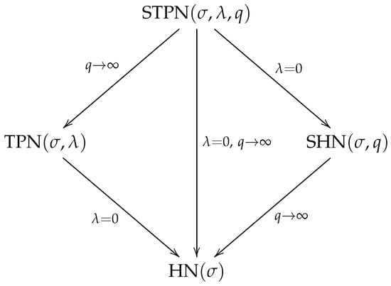
Figure 1. Particular cases for the STPN distribution.

2.2. Density Function

Proposition 1.

Let $Y\sim STPN(\sigma ,\lambda ,q)$. Then, the pdf of Y is given by:

$$f_Y(y;\sigma ,\lambda ,q)=\frac{q}{\sigma \Phi \left(\lambda \right)}{\int }_0^1{w}^q\varphi \left(\frac{yw}{\sigma }-\lambda \right)dw,y>0,$$

(5)

where $\sigma >0$ is a scale parameter, $\lambda \in \mathbb{R}$ is a shape parameter, and $q>0$ is a parameter related to the kurtosis of the distribution.

Proof. 

Using the representation in (4) and computing the Jacobian of the transformation for $Y=Z/U^{1/q}$ and $W=U^{1/q}$, we obtain:

$$\left.\begin{array}{c}Z=YW\hfill \\ U=W^q\hfill \end{array}\right\}\Rightarrow J=\left|\begin{array}{cc}\frac{\partial Z}{\partial Y}\hfill & \frac{\partial Z}{\partial W}\hfill \\ \frac{\partial U}{\partial Y}\hfill & \frac{\partial U}{\partial W}\hfill \end{array}\right| = \left|\begin{array}{cc}w\hfill & z\hfill \\ 0\hfill & q{w}^{q-1}\hfill \end{array}\right|=q{w}^q.$$

Therefore,

$$\begin{array}{cc}\hfill f_{Y,W}(y,w)& =\left|J\right|f_{Z,U}(yw,w^q)=q{w}^q{f}_X\left(yw\right)f_U\left(w^q\right),\hfill \\ \hfill & =\frac{q}{\sigma \Phi \left(\lambda \right)}{w}^q\varphi \left(\frac{yw}{\sigma }-\lambda \right),0<w<1,z>0.\hfill \end{array}$$

Marginalizing with respect to variable W, we obtain the density function corresponding to the rv Y, that is,

$$\begin{array}{ccc}{f}_Y(y;\sigma ,\lambda ,q)& =& {\displaystyle \frac{q}{\sigma \Phi \left(\lambda \right)}{\int }_0^1{w}^q\varphi \left(\frac{yw}{\sigma }-\lambda \right)dw.}\end{array}$$

An alternative way to obtain this pdf is by substituting $u=\frac{yw}{\sigma }-\lambda$, obtaining:

$$f_Y(y;\sigma ,\lambda ,q)=\frac{q{\sigma }^q}{{\left(2\pi \right)}^{1/2}\Phi \left(\lambda \right)y^{q+1}}{\int }_{-\lambda }^{y/\sigma -\lambda }{(u+\lambda )}^q{e}^{-u^2/2}du.$$

With $t=\frac{u^2}{2}$ in the last expression, we obtain:

$${\displaystyle f_Y(y;\sigma ,\lambda ,q)=\frac{q{\sigma }^q}{{\left(2\pi \right)}^{\frac{1}{2}}\Phi \left(\lambda \right)y^{q+1}}\sum _{K=0}^{\infty }\left(\genfrac{}{}{0pt}{}{q}{k}\right){\lambda }^{q-k}{2}^{\frac{k}{2}-\frac{1}{2}}\Gamma \left(\frac{k+1}{2}\right)\left[G\left({\left(\frac{y}{\sigma }-\lambda \right)}^2,\frac{k+1}{2},1\right)-G\left(\frac{{\lambda }^2}{2},\frac{k+1}{2},1\right)\right]}.$$

   □

2.3. Some Properties

In this section, we study some basic properties of the STPN distribution.

Proposition 2.

Let $Y\sim STPN(\sigma ,\lambda ,q)$. Then, the cdf of Y is given by:

$$F_Y(y;\sigma ,\lambda ,q)=\frac{q}{\Phi \left(\lambda \right)}{\int }_0^1{w}^{q-1}\left(\Phi \left(\frac{yw}{\sigma }-\lambda \right)+\Phi \left(\lambda \right)-1\right)dw,y>0$$

Proof. 

It is immediate from the definition.    □

Proposition 3.

Let $Y\sim STPN(\sigma ,\lambda ,q)$. Then, the hazard function is given by:

$$H_Y(y;\sigma ,\lambda ,q)=\frac{\frac{q}{\sigma \Phi \left(\lambda \right)}{\int }_0^1{w}^q\varphi \left(\frac{yw}{\sigma }-\lambda \right)dw}{1-\frac{q}{\Phi \left(\lambda \right)}{\int }_0^1{w}^{q-1}\left(\Phi \left(\frac{yw}{\sigma }-\lambda \right)+\Phi \left(\lambda \right)-1\right)dw},y>0$$

Figure 2 shows the pdf, cdf, and hazard function for the STPN model with different combinations of parameters.

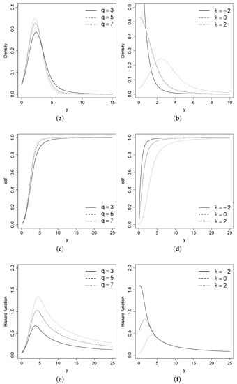
Figure 2. pdf, cdf, and hazard function for the STPN$(\sigma =1,\lambda =2,q)$ model with different combinations of q and the STPN$(\sigma =1,\lambda ,q=2)$ model with different combinations of $\lambda$. (a) pdf of STPN$(\sigma =1,\lambda =2,q)$. (b) pdf of STPN$(\sigma =1,\lambda ,q=2)$. (c) cdf of STPN$(\sigma =1,\lambda =2,q)$. (d) cdf of STPN$(\sigma =1,\lambda ,q=2)$. (e) hazard function of STPN$(\sigma =1,\lambda =2,q)$. (f) hazard function of STPN$(\sigma =1,\lambda ,q=2)$.

Proposition 4.

Let $Y\sim STPN(\sigma ,\lambda ,q)$. If $q\to +\infty$, then Y strongly converges to the rv $Z\sim TPN(\sigma ,\lambda )$.

Proof. 

Let $Y\sim \mathrm{STPN}(\sigma ,\lambda ,q)$. Then, Y can be written as $Y=Z/U^{1/q}$, where $Z\sim \mathrm{TPN}(\sigma ,\lambda )$ and $U\sim U(0,1)$. First, we studied the convergence in the probability of $U^{1/q}$. It is clear that $W=U^{1/q}$, then $W\sim Beta(q,1)$, so that $E{(W-1)}^2=\frac{2}{(q+1)(q+2)}$. If $q\to +\infty$, then $E{(W-1)}^2\to 0$. Therefore,

$$W=U^{1/q}\stackrel{\mathcal{P}}{\to }1,\mathrm{as}q\to +\infty ,$$

where $\stackrel{\mathcal{P}}{\to }$ denotes convergence in probability. Then, applying Slutsky’s theorem [16] to $Y=Z/U^{1/q}$, we have:

$$Y\stackrel{\mathcal{D}}{\to }Z,\mathrm{as}q\to +\infty ,$$

where $\stackrel{\mathcal{D}}{\to }$ denotes convergence in the distribution. In other words, for greater q values, Y strongly converges to the $TPN(\sigma ,\lambda )$ distribution.

   □

Proposition 5.

If $Y|T=t\sim TPN(\sigma t^{-1/q},\lambda )$ and $T\sim U(0,1)$, then $Y\sim STPN(\sigma ,\lambda ,q).$

Proof. 

The marginal distribution of Y can be computed as:

$$f_Y(y;\sigma ,\lambda ,q)={\int }_0^1{f}_{Y|T}\left(y\right|t)f_T\left(t\right)dt={\int }_0^1\frac{1}{\sigma \Phi \left(\lambda \right)t^{-1/q}}\varphi \left(\frac{y}{\sigma t^{-1/q}}-\lambda \right)dt.$$

With the transformation $w=t^{1/q}$, we obtain Equation (5).    □

Remark 1.

Proposition 4 implies that for $q\to +\infty$, the pdf of the STPN distribution converges to the pdf of the TPN model. Proposition 5 shows that the STPN distribution can also be seen as a scale mixture of the TPN model. This property is very important for obtaining random values from this model and for the application of an EM-type algorithm to estimate the parameters of the model.

2.4. Moments

The following proposition provides the moments of the STPN distribution.

Proposition 6.

Let $Y\sim STPN(\sigma ,\lambda ,q)$. Therefore, for $r=1,2,\dots$ and $q>r$, the r-th moment of Y is given by:

$${\mu }_r=E\left(Y^r\right)=\frac{q{\sigma }^r}{q-r}{\kappa }_r\left(\lambda \right),$$

where ${\kappa }_r\left(\lambda \right)=\frac{1}{\sqrt{2\pi }\Phi \left(\lambda \right)}{\sum }_{k=0}^t\left(\genfrac{}{}{0pt}{}{r}{k}\right){\lambda }^{r-k}{2}^{(k-1)/2}\Gamma ((k+1),{\lambda }^2/2)$.

Proof. 

Using the stochastic representation given in Equation (4), we have that:

$${\mu }_r=E\left(Y^r\right)=E\left(Z^r{U}^{-r/q}\right)=E\left(Z^r\right)E\left(U^{-r/q}\right),$$

where $E\left(U^{-r/q}\right)=\frac{q}{q-r}$, $q>r$, and ${\displaystyle E\left(Z^r\right)=\frac{{\sigma }^r}{\sqrt{2\pi }\Phi \left(\lambda \right)}\sum _{k=0}^t\left(\genfrac{}{}{0pt}{}{r}{k}\right){\lambda }^{r-k}{2}^{(k-1)/2}\Gamma ((k+1),{\lambda }^2/2)}$ are the moments of the TPN$(\sigma ,\lambda )$ model.    □

Corollary 1.

If $Y\sim STPN(\sigma ,\lambda ,q)$, then its first four moments are determined as follows:

• ${\mu }_1=E\left(Y\right)=\frac{q\sigma }{q-1}{\kappa }_1\left(\lambda \right),q>1;$
• ${\mu }_2=E\left(Y^2\right)=\frac{q{\sigma }^2}{q-2}{\kappa }_2\left(\lambda \right),q>2;$
• ${\mu }_3=E\left(Y^3\right)=\frac{q{\sigma }^3}{q-3}{\kappa }_3\left(\lambda \right),q>3;$
• ${\mu }_4=E\left(Y^4\right)=\frac{q{\sigma }^4}{q-4}{\kappa }_4\left(\lambda \right),q>4.$

$$Var\left(Y\right)={\sigma }^{2}q\left(\frac{1}{q-2}{\kappa }_2\left(\lambda \right)-\frac{q}{{(q-1)}^2}{\kappa }_1^2\left(\lambda \right)\right),q>2.$$

(6)

Proof. 

It is immediate from Proposition 6.    □

Corollary 2.

Let $Y\sim STPN(\sigma ,\lambda ,q)$, then the asymmetry coefficient $\left(\sqrt{{\beta }_1}\right)$ and the kurtosis coefficient $\left({\beta }_2\right)$ are:

$$\sqrt{{\beta }_1}=\frac{\sqrt{q-2}\{{(q-1)}^3(q-2){\kappa }_3-3q{\kappa }_1{\kappa }_2{(q-1)}^2(q-3)+2q^2(q-2)(q-3){\kappa }_1^3\}}{\sqrt{q}(q-3){\{{(q-1)}^2{\kappa }_2-q(q-2){\kappa }_1^2\}}^{3/2}},q>3,$$

(7)

$${\beta }_2=\frac{{(q-1)}^3{(q-2)}^{2}A+3(q-2)(q-3)(q-4)q^{2}B}{q(q-3)(q-4){\{{(q-1)}^2{\kappa }_2-q(q-2){\kappa }_1^2\}}^2},q>4$$

(8)

where $A=(q-3)(q-1){\kappa }_4-4q(q-1)(q-4){\kappa }_1{\kappa }_3$ and $B=2{(q-1)}^2{\kappa }_1^2{\kappa }_2-q(q-2){\kappa }_1^4$.

Proof. 

By the definition of the asymmetry and kurtosis coefficients, we have:

$$\sqrt{{\beta }_1}=\frac{{\mu }_3-3{\mu }_2{\mu }_1+2{\mu }_1^3}{{({\mu }_2-{\mu }_1^2)}^{3/2}}and{\beta }_2=\frac{{\mu }_4-4{\mu }_1{\mu }_3+6{\mu }_1^2{\mu }_2-3{\mu }_1^4}{{({\mu }_2-{\mu }_1^2)}^2}.$$

Replacing ${\mu }_1,{\mu }_2,{\mu }_3$, and ${\mu }_4$ obtained in Corollary 1, we have the result.    □

Remark 2.

Proposition 6 shows that the moments of the $STPN$ distribution depend essentially on the moments of the $TPN$ distribution. Equations (6) and (8) show the effect of parameter q on the model; a lower value of q produces greater variance and kurtosis. Table 1 shows some values of the kurtosis coefficient of the $STPN$ distribution for different values of λ and q.

Table 1. Some values for the kurtosis coefficients of the STPN distribution for different values of $\lambda$ and q.

	q
$\mathit{\lambda }$	5	7	10	15	$+\mathit{\infty }$ (TPN)
−5	19.68	10.28	8.58	8.04	7.76
−2	16.63	8.22	6.73	6.26	6.02
−1	14.88	7.02	5.64	5.22	5.00
0	13.19	5.72	4.45	4.06	3.87
1	12.70	4.82	3.54	3.18	3.00
2	15.23	4.93	3.34	2.93	2.76
5	35.37	10.07	4.84	3.44	2.99

Figure 3 shows the mean, standard deviation, asymmetry coefficient, and kurtosis coefficient for the STPN$(\sigma =1,\lambda ,q)$ in terms of $\lambda$ and q.

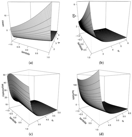
Figure 3. (a) Mean; (b) standard deviation; (c) asymmetry coefficient; (d) kurtosis coefficient for the STPN($\lambda ,\sigma =1,q$) model.

3. Inference

In this Section, we discuss a classical approach for the inference for the STPN distribution. In particular, we discuss the moments estimators and maximum likelihood (ML) estimation based on the EM algorithm.

3.1. Moments Estimators

The moments estimators result from the solution of the equation $E\left(Y^j\right)=\overline{Y^j}$, for $j=1,2,3$, where $\overline{Y^j}=n^{-1}{\sum }_{i=1}^n{y}_i^j$ denotes the j-th sample moment. Solving $E\left(Y\right)=\overline{Y}$, we have that:

$$\begin{array}{cc}\hfill \sigma & =\frac{(q-1)\overline{Y}}{q(\lambda +\xi (\lambda \left)\right)}.\end{array}$$

(9)

Replacing this, we have the following nonlinear equations

$$\begin{array}{ccc}\hfill \overline{Y^2}& =& \frac{{\overline{Y}}^2{(q-1)}^2({\lambda }^2+\lambda \xi \left(\lambda \right)+1)}{q(q-2){(\lambda +\xi \left(\lambda \right))}^2},\mathrm{and}\hfill \\ \hfill \overline{Y^3}& =& \frac{{\overline{Y}}^3{(q-1)}^3({\lambda }^3+{\lambda }^2\xi \left(\lambda \right)+3\lambda +2\xi \left(\lambda \right))}{q^2(q-3){(\lambda +\xi \left(\lambda \right))}^3}.\hfill \end{array}$$

These equations can be solved using different software. For instance, in R [17], we can use the nleqslv function to obtain the moments estimators ${\widehat{\lambda }}_M$ and ${\widehat{q}}_M$. The moments estimator ${\widehat{\sigma }}_M$ is obtained by substitution in Equation (9).

3.2. Maximum Likelihood Estimation

Given $y_1,\dots ,y_n$, a random sample from the STPN$(\sigma \lambda ,q)$ distribution, the log-likelihood function for $\mathbf{\theta }=(\sigma ,\lambda ,q)$ is given by:

$$\ell \left(\mathbf{\theta }\right)=nlog\left(q\right)-nlog\left(\sigma \right)-nlog(\Phi \left(\lambda \right))+\sum _{i=1}^{n}log\left(G\left(y_i\right)\right),$$

where:

$$G\left(y_i\right)=G(y_i,\sigma ,\lambda ,q)={\int }_0^1{w}^q\varphi \left(\frac{y_{i}w}{\sigma }-\lambda \right)dw.$$

Deriving in relation to the components of $\mathbf{\theta }$, we obtain the following ML equations:

$$\sum _{i=1}^n\frac{G_1\left(y_i\right)}{G\left(y_i\right)}=\frac{n}{\sigma },\sum _{i=1}^n\frac{G_2\left(y_i\right)}{G\left(y_i\right)}=n\xi \left(\lambda \right),\mathrm{and}-\sum _{i=1}^n\frac{G_3\left(y_i\right)}{G\left(y_i\right)}=\frac{n}{q},$$

where $G_1\left(y_i\right)=\frac{\partial G\left(y_i\right)}{\partial \sigma }$, $G_2\left(y_i\right)=\frac{\partial G\left(y_i\right)}{\partial \lambda }$, and $G_3\left(y_i\right)=\frac{\partial G\left(y_i\right)}{\partial q}$. For $j>0$, we define:

$$\begin{array}{cc}\hfill a_i\left(j\right)& =a_i(\sigma ,\lambda ,j)={\int }_0^1{w}^j\varphi \left(\frac{y_{i}w}{\sigma }-\lambda \right)dw,\mathrm{and}\hfill \\ \hfill b_i\left(j\right)& =b_i(\sigma ,\lambda ,j)={\int }_0^1{w}^{j}ln\left(w\right)\varphi \left(\frac{y_{i}w}{\sigma }-\lambda \right)dw.\hfill \end{array}$$

With those notations, the ML equations can also be written as:

$$\begin{array}{ccc}\hfill \sum _{i=1}^n\frac{y_i^2}{{\sigma }^3}\frac{a_i(q+2)}{a_i\left(q\right)}-\sum _{i=1}^n\frac{y_i\lambda }{{\sigma }^2}\frac{a_i(q+1)}{a_i\left(q\right)}& =& \frac{n}{\sigma },\hfill \\ \hfill \sum _{i=1}^n\frac{y_i}{\sigma }\frac{a_i(q+1)}{a_i\left(q\right)}-n\lambda & =& n\xi \left(\lambda \right),\mathrm{and}\hfill \\ \hfill \sum _{i=1}^n\frac{b_i\left(q\right)}{a_i\left(q\right)}& =& -\frac{n}{q}\hfill \end{array}$$

Taking $x_i=y_i/\sigma$, ${\omega }_1\left(x_i\right)=\frac{a_i(q+2)}{a_i\left(q\right)}$, ${\omega }_2\left(x_i\right)=\frac{b_i\left(q\right)}{a_i\left(q\right)}$, and ${\omega }_3\left(x_i\right)=\frac{a_i(q+1)}{a_i\left(q\right)}$, the equations are equivalent to:

$$\sum _{i=1}^n{x}_i^2{\omega }_1\left(x_i\right)-\lambda \sum _{i=1}^n{x}_i{\omega }_3\left(x_i\right)=n,\sum _{i=1}^n\frac{y_i}{\sigma }{\omega }_3\left(x_i\right)-n\lambda =n\xi \left(\lambda \right),\mathrm{and}\sum _{i=1}^n{\omega }_2\left(x_i\right)=-\frac{n}{q}.$$

The ML estimators can be obtained directly using numerical procedures. However, to increase the robustness of the procedure for obtaining those estimators, we also discuss an EM-type algorithm for estimation in the model.

3.3. EM Algorithm

The EM algorithm is a well-known tool for ML estimation in the presence of nonobserved (latent) data. For this particular problem, the algorithm takes advantage of the stochastic representation of the STPN model in Equation (4). Let $W=U^{1/q}$. The representation of the model can be seen as $Y_i=Z_i/W_i$, where $W_i\sim$ Beta$(q,1)$.

In this context, the STPN distribution can also be written using the following hierarchical representation:

$$\begin{array}{ccc}\hfill Y_i|W_i=w_i& \stackrel{ind.}{\sim }& TPN\left(\frac{\sigma }{w_i},\lambda \right),\hfill \\ \hfill W_i& \stackrel{ind.}{\sim }& Beta(q,1),i=1,\dots n.\hfill \end{array}$$

In our context, $\mathbf{y}={[y_1,\dots ,y_n]}^{\top }$ and $\mathbf{w}={[w_1,\dots ,w_n]}^{\top }$ represent the observed and nonobserved data, respectively. The complete data are given by ${\mathbf{y}}_c=[{\mathbf{y}}^{\top },{\mathbf{w}}^{\top }]$. We also denote ${\ell }_c\left(\theta \right|{\mathbf{y}}_c)$ as the complete log-likelihood function, which up to a constant is given by:

$$\begin{array}{c}\hfill {\ell }_c\left(\theta \right|{\mathbf{y}}_c)=n\left[logq-log\left(\sigma \right)-log(\Phi (\lambda \left)\right)\right]-\frac{n}{2}{\lambda }^2-\sum _{i=1}^n\frac{y_i^2{w}_i^2}{2{\sigma }^2}+\frac{\lambda }{\sigma }\sum _{i=1}^n{y}_i{w}_i+q\sum _{i=1}^{n}log\left(w_i\right).\end{array}$$

Note that $Q(\theta |{\widehat{\theta }}^{(k)})=E({\ell }_c(\theta |\mathbf{y})|\mathbf{y},\mathbf{\theta }={\widehat{\theta }}^{(k)})$; the expected value of ${\ell }_c\left(\theta \right)$ provided the observed data is given by:

$$\begin{array}{cc}\hfill Q(\theta |{\widehat{\theta }}^{\left(k\right)})& =n\left[logq-log\left(\sigma \right)-log(\Phi (\lambda \left)\right)\right]-\frac{n}{2}{\lambda }^2-\sum _{i=1}^n\frac{y_i^2{\widehat{w_i^2}}^{\left(k\right)}}{2{\sigma }^2}+\frac{\lambda }{\sigma }\sum _{i=1}^n{y}_i{\widehat{w_i}}^{\left(k\right)}\hfill \\ \hfill & +q\sum _{i=1}^n{\widehat{log{w}_i}}^{\left(k\right)},\hfill \end{array}$$

where ${\widehat{w_i}}^{\left(k\right)}=E(w_i|y_i,\theta ={\widehat{\theta }}^{\left(k\right)})$, ${\widehat{w_i^2}}^{\left(k\right)}=E(w_i^2|y_i,\theta ={\widehat{\theta }}^{\left(k\right)})$, and ${\widehat{log{w}_i}}^{\left(k\right)}=E(log{w}_i|y_i,$$\theta ={\widehat{\theta }}^{\left(k\right)})$. In our context, ${\widehat{w}}_i^{\left(k\right)}$, ${\widehat{w}}_i^2$${}^{\left(k\right)}$ and ${\widehat{log{w}_i}}^{\left(k\right)}$ do not have a closed form; they therefore need to be computed numerically. In short, the k-th step of the EM algorithm is detailed as follows:

• E-step: For ${\widehat{\theta }}^{\left(k\right)}={({\widehat{\sigma }}^{\left(k\right)},{\widehat{\lambda }}^{\left(k\right)},{\widehat{q}}^{\left(k\right)})}^{\top }$, the value for the vector of parameters at the k-step, compute ${\widehat{w}}_i^{\left(k\right)}$, ${\widehat{w}}_i^2$${}^{\left(k\right)}$, and ${\widehat{log{w}_i}}^{\left(k\right)}$, for $i=1,\dots ,n$;
• CM-Step I: Given ${\widehat{\lambda }}^{\left(k\right)}$ and ${\widehat{w}}_1^{\left(k\right)},\dots ,{\widehat{w}}_n^{\left(k\right)}$, update $\sigma$ as follows:

  $${\widehat{\sigma }}^{(k+1)}=\frac{{\sum }_{i=1}^n{y}_i{\widehat{w}}_i^{\left(k\right)}}{n\xi \left({\widehat{\lambda }}^{\left(k\right)}\right)+n{\widehat{\lambda }}^{\left(k\right)}};$$
• CM-Step II: Given ${\widehat{\sigma }}^{(k+1)}$ and ${\widehat{w}}_1^{\left(k\right)},\dots ,{\widehat{w}}_n^{\left(k\right)}$, update $\lambda$ since the solution is obtained from the nonlinear equation.

  $$-\frac{{\sum }_{i=1}^n{y}_i{\widehat{w}}_i^{\left(k\right)}}{n}=\xi {\left({\widehat{\lambda }}^{\left(k\right)}\right)}^2+3\xi \left({\widehat{\lambda }}^{\left(k\right)}\right){\widehat{\lambda }}^{\left(k\right)}+2{\widehat{\lambda }}^{2^{\left(k\right)}};$$
• CM-Step III: Given ${\widehat{log{w}_1}}^{\left(k\right)},\dots ,{\widehat{log{w}_n}}^{\left(k\right)}$, update q as follows:

  $${\widehat{q}}^{(k+1)}=-\frac{n}{{\sum }_{i=1}^n{\widehat{log{w}_i}}^{\left(k\right)}}.$$

The E-, CM-I, CM-II, and CM-III steps are repeated until an ad hoc criterion is satisfied. For instance, we considered $\left|\ell ({\widehat{\theta }}^{(k+1)})-\ell ({\widehat{\theta }}^{\left(k\right)})\right|<ϵ$, for a fixed $ϵ$. In other words, the difference in the observed log-likelihood for successive steps is lower than a determined value. The initial values for the algorithm can be obtained, for instance, using the ${\widehat{\sigma }}_M$, ${\widehat{\lambda }}_M$, and ${\widehat{q}}_M$, moments estimators.

3.4. Observed Fisher Information Matrix

The variance of the estimators can be estimated based on the observed Fisher information matrix, say $\mathcal{I}\left(\mathbf{\theta }\right)=-{\partial }^2\ell \left(\mathbf{\theta }\right)/\partial \mathbf{\theta }\partial {\mathbf{\theta }}^{\top }$. In particular, we have that:

$$\sqrt{n}\mathcal{I}{\left(\mathbf{\theta }\right)}^{-1}\left(\mathbf{\theta }-\widehat{\mathbf{\theta }}\right)\stackrel{\mathcal{D}}{\to }{N}_3({\mathbf{0}}_3,{\mathbf{I}}_3),\mathrm{as} n\to +\infty ,$$

where $N_3({\mathbf{0}}_3,{\mathbf{I}}_3)$ denotes the standard trivariate normal distribution. The computation of $\mathcal{I}\left(\mathbf{\theta }\right)$ is not trivial, because it involves the derivation of functions that depend on integrals. Taking advantage of the complete log-likelihood function, $\mathcal{I}\left(\mathbf{\theta }\right)$ can also be approximated by Louis’ method [14] as follows:

$$\begin{array}{cc}\hfill \mathcal{I}\left(\mathbf{\theta }\right)& =\sum _{i=1}^{n}E\left({\mathbf{B}}_i\left(\mathbf{\theta }\right)|\mathbf{y},\mathbf{\theta }=\widehat{\mathbf{\theta }}\right)-\sum _{i=1}^{n}E\left({\mathbf{S}}_i\left(\mathbf{\theta }\right){\mathbf{S}}_i^{\top }\left(\mathbf{\theta }\right)|\mathbf{y},\mathbf{\theta }=\widehat{\mathbf{\theta }}\right)\hfill \\ \hfill & +\underset{\begin{array}{c}1\le i,j\le n\\ i\ne j\end{array}}{\sum \sum }E\left({\mathbf{S}}_i\left(\mathbf{\theta }\right)\mid \mathbf{y},\mathbf{\theta }=\widehat{\mathbf{\theta }}\right)E^{\top }\left({\mathbf{S}}_j\left(\mathbf{\theta }\right)\mid \mathbf{y},\mathbf{\theta }=\widehat{\mathbf{\theta }}\right).\hfill \end{array}$$

The details of the components of $\mathcal{I}\left(\mathbf{\theta }\right)$ are provided in the Appendix A.

3.5. Computational Aspects

The EM algorithm and Louis’ method to obtain the ML estimators and their standard errors for the STPN distribution are included in the tpn package [18] from R [17]. The following function can be used to obtain these results:

est.stpn(y, sigma0=NULL, lambda0=NULL, q0=NULL, prec = 0.001, max.iter = 1000)

where y is the response variable, sigma0, lambda0, q0 are the initial values for the algorithm (they are not defined by default), prec is the precision for the parameters, and max.iter is the maximum number of iterations to be applied for the algorithm. The tpn package also includes the functions dstpn, pstpn, and rstpn, which compute the pdf, cdf, and generation for the STPN distribution.

4. Simulation

In this section, we study the performance of the ML estimators using the EM algorithm for the STPN distribution under different scenarios. We considered two values for $\sigma$: 2 and 10; three values for $\lambda$: −1, 1, and 3; two values for q: $-1.5$ and 3; and four sample sizes: 50, 100, 200, and 500. For each combination of $\sigma ,\lambda ,q$ and n (totaling 48 combinations), we drew 1000 replicates, and we used the tpn package to estimate the parameters based on the EM algorithm and estimated the standard deviations based on Louis’ method to estimate the observed Fisher information matrix. Table 2 summarizes the mean of the estimated bias for the 1000 replicates (bias), the mean of the standard errors (SEs), the root of the estimated mean-squared error (RMSE), and the estimated coverage probability based on the asymptotic distribution for the ML estimator using a 95% confidence level (CP). Note that the bias and the RMSE terms are reduced when the sample size is increased, suggesting that the estimators are consistent even in finite samples. The SE and RMSE terms are closer when the sample size is increased, suggesting that the standard errors are also consistently estimated. Finally, the CP terms converges to the nominal value when the sample size is increased, suggesting that the asymptotic distribution of the ML estimators also works well in finite samples.

Table 2. Recovery parameters for the STPN distribution based on 1000 replicates for different combinations of parameters and sample size.

True Value				$\mathit{n}=50$				$\mathit{n}=100$				$\mathit{n}=200$				$\mathit{n}=500$
$\mathbf{\sigma }$	$\mathbf{\lambda }$	$\mathbf{q}$	est.	bias	SE	RMSE	CP	bias	SE	RMSE	CP	bias	SE	RMSE	CP	bias	SE	RMSE	CP
2	−1	1.5	$\widehat{\sigma }$	−0.43	1.98	1.06	0.71	−0.12	1.98	1.09	0.80	0.04	1.64	1.01	0.88	0.19	1.17	0.81	0.92
			$\widehat{\lambda }$	0.76	2.29	1.40	0.77	0.33	2.10	1.21	0.83	0.11	1.69	1.02	0.90	−0.14	1.20	0.83	0.94
			$\widehat{q}$	0.09	0.57	0.54	0.94	0.08	0.42	0.43	0.93	0.06	0.29	0.32	0.96	0.03	0.18	0.16	0.97
		3	$\widehat{\sigma }$	−0.70	1.28	0.97	0.62	−0.34	1.30	0.86	0.78	−0.09	1.13	0.78	0.86	0.07	0.78	0.66	0.94
			$\widehat{\lambda }$	0.94	1.64	1.35	0.72	0.45	1.49	1.08	0.83	0.19	1.18	0.85	0.90	−0.05	0.81	0.68	0.94
			$\widehat{q}$	−0.30	2.11	2.01	0.81	−0.11	1.50	1.03	0.88	0.08	1.23	0.93	0.93	0.09	0.72	0.67	0.93
	1	1.5	$\widehat{\sigma }$	0.21	1.18	1.14	0.89	0.20	0.80	0.86	0.94	0.09	0.49	0.50	0.95	0.06	0.29	0.31	0.96
			$\widehat{\lambda }$	0.06	0.76	0.72	0.94	−0.04	0.53	0.52	0.96	−0.02	0.35	0.35	0.97	−0.02	0.22	0.22	0.95
			$\widehat{q}$	0.23	0.63	0.72	0.96	0.10	0.33	0.39	0.96	0.04	0.21	0.25	0.96	0.03	0.13	0.14	0.95
		3	$\widehat{\sigma }$	−0.01	0.83	0.67	0.88	0.09	0.58	0.53	0.94	0.07	0.39	0.41	0.95	0.03	0.23	0.24	0.95
			$\widehat{\lambda }$	0.11	0.60	0.56	0.95	0.01	0.41	0.39	0.96	−0.01	0.29	0.30	0.96	−0.01	0.18	0.18	0.96
			$\widehat{q}$	1.07	4.79	5.13	0.92	0.46	1.53	1.36	0.95	0.28	0.81	0.89	0.96	0.11	0.42	0.46	0.97
	3	1.5	$\widehat{\sigma }$	0.12	0.59	0.83	0.94	0.04	0.37	0.40	0.95	0.02	0.26	0.25	0.96	0.03	0.17	0.17	0.95
			$\widehat{\lambda }$	0.13	0.70	0.76	0.95	0.07	0.45	0.63	0.95	0.02	0.31	0.30	0.96	−0.02	0.19	0.19	0.95
			$\widehat{q}$	0.14	0.39	0.50	0.96	0.06	0.22	0.23	0.97	0.03	0.16	0.16	0.95	0.02	0.10	0.10	0.95
		3	$\widehat{\sigma }$	0.01	0.45	0.48	0.95	0.04	0.31	0.31	0.96	0.02	0.21	0.21	0.96	0.01	0.13	0.13	0.95
			$\widehat{\lambda }$	0.16	0.57	0.63	0.97	0.02	0.37	0.37	0.96	0.02	0.25	0.25	0.95	0.01	0.16	0.16	0.95
			$\widehat{q}$	0.50	1.55	2.01	0.96	0.22	0.67	0.78	0.96	0.11	0.43	0.48	0.96	0.05	0.26	0.25	0.97
10	−1	1.5	$\widehat{\sigma }$	−2.41	8.09	5.04	0.70	−1.37	7.73	4.63	0.76	−1.00	5.71	3.71	0.83	0.05	4.56	3.03	0.90
			$\lambda$	0.84	1.89	1.34	0.75	0.52	1.71	1.08	0.81	0.34	1.25	0.85	0.86	0.04	0.97	0.66	0.92
			$\widehat{q}$	0.08	0.56	0.55	0.92	0.07	0.41	0.45	0.93	0.03	0.27	0.27	0.94	0.02	0.17	0.16	0.97
		3	$\widehat{\sigma }$	−3.69	5.49	4.83	0.62	−2.29	5.30	3.86	0.76	−0.93	4.73	3.14	0.85	0.11	3.58	2.87	0.90
			$\widehat{\lambda }$	0.99	1.45	1.33	0.71	0.58	1.27	0.98	0.82	0.28	1.03	0.74	0.88	0.04	0.75	0.60	0.92
			$\widehat{q}$	−0.30	2.05	2.03	0.81	−0.19	1.33	0.95	0.87	0.07	1.18	0.92	0.92	0.15	0.76	0.73	0.94
	1	1.5	$\widehat{\sigma }$	1.24	6.09	5.89	0.89	0.87	3.89	4.52	0.93	0.37	2.40	2.66	0.93	0.25	1.42	1.49	0.95
			$\widehat{\lambda }$	0.02	0.77	0.72	0.95	−0.02	0.52	0.52	0.96	−0.00	0.35	0.37	0.95	−0.02	0.21	0.22	0.96
			$\widehat{q}$	0.23	0.59	0.68	0.97	0.12	0.36	0.45	0.95	0.04	0.21	0.23	0.96	0.02	0.13	0.13	0.95
		3	$\widehat{\sigma }$	−0.11	3.87	3.17	0.89	0.26	2.84	2.60	0.92	0.28	1.91	2.02	0.94	0.14	1.14	1.21	0.95
			$\widehat{\lambda }$	0.12	0.59	0.54	0.95	0.03	0.41	0.39	0.94	0.00	0.28	0.28	0.95	−0.00	0.18	0.18	0.95
			$\widehat{q}$	1.28	5.65	6.16	0.91	0.41	1.55	1.75	0.94	0.30	0.87	1.03	0.96	0.10	0.42	0.45	0.97
	3	1.5	$\widehat{\sigma }$	0.44	2.74	3.03	0.93	0.22	1.85	1.91	0.95	0.15	1.27	1.36	0.94	0.09	0.81	0.85	0.95
			$\widehat{\lambda }$	0.14	0.67	0.89	0.96	0.05	0.44	0.47	0.96	0.02	0.30	0.31	0.96	−0.00	0.19	0.20	0.95
			$\widehat{q}$	0.14	0.35	0.42	0.98	0.06	0.23	0.24	0.96	0.03	0.15	0.16	0.96	0.01	0.10	0.10	0.95
		3	$\widehat{\sigma }$	0.22	2.24	2.36	0.94	0.07	1.50	1.57	0.94	0.00	1.03	1.06	0.95	0.01	0.65	0.65	0.95
			$\widehat{\lambda }$	0.11	0.55	0.59	0.97	0.07	0.37	0.40	0.97	0.04	0.25	0.26	0.95	0.01	0.16	0.16	0.95
			$\widehat{q}$	0.69	1.98	3.14	0.95	0.21	0.67	0.82	0.96	0.10	0.42	0.45	0.96	0.04	0.25	0.26	0.96

5. Application

In this section, we present a real data application in order to illustrate the performance of the STPN model in comparison with other proposals in the literature. For this, a comparison was conducted utilizing the TPN distribution and the model proposed by Gómez et al. [19], which is a generalization of a TPN model, denominated the generalized TPN (GTPN). The density function of the GPTN model is given by:

$$f(y;\sigma ,\lambda ,\alpha )=\frac{\alpha }{{\sigma }^{\alpha }\Phi \left(\lambda \right)}{y}^{\alpha -1}\varphi \left({\left(\frac{y}{\sigma }\right)}^{\alpha }-\lambda \right),$$

with $x>0$, $\sigma ,\alpha >0$, and $\lambda \in \mathbb{R}$.

A real dataset of body fat was considered, which measured weight and various body circumferences (see http://lib.stat.cmu.edu/datasets/bodyfat (accessed on 8 October 2021)); for examination purposes, the weight variable (measured in pounds (lbs)) was chosen to conduct the application. When calculating basic statistics (Table 3 shows basic statistics), high kurtosis can be observed for the variable, suggesting the use of a distribution with heavy tails as the STPN.

Table 3. Descriptive statistics for the $weight$ dataset.

Dataset	n	$\overline{\mathit{X}}$	${\mathit{S}}^2$	$\sqrt{{\mathit{b}}_1}$	${\mathit{b}}_2$
Weight measured	252	$178.9$	$863.72$	$1.2$	$8.14$

Table 4 shows the estimated parameters for the three models considered. Based on the AIC [20] and BIC [21], the STPN model provides a better fit. In addition, Figure 4 shows the histogram for the data and the estimated pdf for all the models, where a better performance of the STPN model is shown. In order to check the better fit of the STPN model in comparison with the rest of the models, we also computed the quantile residuals (QRs). If the model is appropriate for the data, the QRs should be a sample from the standard normal model. This assumption can be validated with traditional normality tests such as the Anderson–Darling (AD), Cramér–von Mises (CVM), and Shapiro–Wilkes (SW) tests. Figure 5 suggests that the STPN model provides a better fit for this dataset.

Table 4. Estimated parameters and their standard errors (in parentheses) for the STPN, TPN, and GTPN models for the $weight$ dataset. The AIC and BIC are also presented.

Estimated	STPN	TPN	GTPN
$\sigma$	20.775 (1.811)	29.331 (1.306)	0.321 (0.088)
$\lambda$	7.825 (0.593)	6.100 (0.279)	14.689 (0.636)
q	11.250 (2.132)	-	-
$\alpha$	-	-	0.426 (0.015)
$AIC$	2394.456	2421.978	2405.15
$BIC$	2405.044	2429.037	2415.738

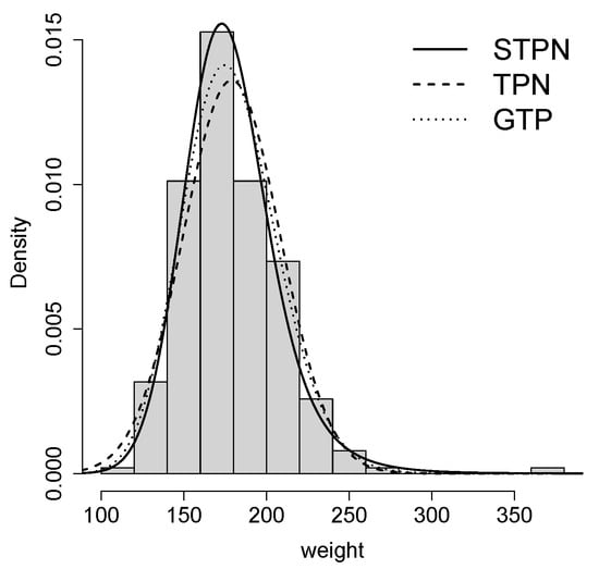
Figure 4. Fit of the distributions for the $weight$ dataset.

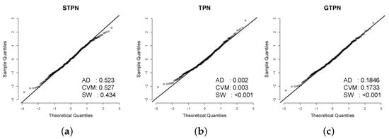
Figure 5. QRs for the fitted models in the $weight$ dataset. The p-values for the AD, CVM, and SW normality tests are also presented to check if the QRs came from the standard normal distribution. (a) qq-plot STPN. (b) qq-plot TPN. (c) qq-plot GTPN.

6. Conclusions

This study presents a new distribution with positive support denominated the slash truncation positive normal. This distribution serves as a more general model compared to the TPN model, pursuing the increase of kurtosis in order to improve the modeling of positive databases with high kurtosis. The basic properties of the model were analyzed, and a simulation study was conducted implementing the EM algorithm. Finally, an application with real data was performed proving that the new model performs better than competing models.

References

- Rafiqullah, H.M.; Saxena, A.; Vera, V.; Abdool-Ghany, F.; Gabbidon, K.; Perea, N.; Shauna-Jeanne Stewart, T.; Ramamoorthy, V. Black Hispanic and Black Non-Hispanic Breast Cancer Survival Data Analysis with Half-normal Model Application. Asian Pac. J. Cancer Prev. 2014, 15, 9453–9458. [Google Scholar]
- Bosch-Badia, M.T.; Montllor-Serrats, J.; Tarrazon-Rodon, M.A. Risk Analysis through the Half-Normal Distribution. Mathematics 2020, 8, 2080. [Google Scholar] [CrossRef]
- Tsizhmovska, N.L.; Martyushev, L.M. Principle of Least Effort and Sentence Length in Public Speaking. Entropy 2021, 23, 1023. [Google Scholar] [CrossRef] [PubMed]
- Olmos, N.M.; Varela, H.; Gómez, H.W.; Bolfarine, H. An extension of the half-normal distribution. Stat. Pap. 2012, 53, 875–886. [Google Scholar] [CrossRef]
- Cooray, K.; Ananda, M.M.A. A generalization of the half-normal distribution with applications to lifetime data. Comm. Stat. Theory Methods 2007, 36, 1323–2157. [Google Scholar] [CrossRef]
- Olmos, N.M.; Varela, H.; Gómez, H.W.; Bolfarine, H. An extension of the generalized half-normal distribution. Stat. Pap. 2014, 55, 967–981. [Google Scholar] [CrossRef]
- Iriarte, Y.; Gómez, H.W.; Varela, H.; Bolfarien, H. Slashed Rayleigd distribution. Rev. Colomb. Estad. 2015, 38, 31–44. [Google Scholar] [CrossRef]
- Reyes, J.; Barranco-Chamorro, I.; Gallardo, D.I.; Gómez, H.W. Generalized modified slash Birnbaum-Saunders distribution. Symmetry 2018, 10, 724. [Google Scholar] [CrossRef] [Green Version]
- Olmos, N.M.; Osvaldo, V.; Gómez, Y.M.; Iriarte, Y.A. Confluent hypergeometric slashed-Rayleigh distribution: Properties, estimation and applications. J. Comput. Appl. Math. 2020, 328, 112548. [Google Scholar] [CrossRef]
- Segovia, F.A.; Gómez, Y.M.; Venegas, O.; Gómez, H.W. A Power Maxwell Distribution with Heavy Tails and Applications. Mathematics 2020, 8, 1116. [Google Scholar] [CrossRef]
- Astorga, J.M.; Reyes, J.; Santoro, K.I.; Venegas, O.; Gómez, H.W. A Reliability Model Based on the Incomplete Generalized Integro-Exponential Function. Mathematics 2020, 8, 1537. [Google Scholar] [CrossRef]
- Gómez, H.J.; Olmos, N.M.; Varela, H.; Bolfarine, H. Inference for a truncated positive normal distribution. Appl. Math. J. Chin. Univ. 2018, 33, 163–176. [Google Scholar] [CrossRef]
- Jonhson, N.L.; Kotz, S.; Balakrishnan, N. Continuos Univariate Distribution, 2nd ed.; Wiley: New York, NY, USA, 1995; Volume 2. [Google Scholar]
- Dempster, A.P.; Laird, N.M.; Rubin, D.B. Maximum Likelihood from Incomplete Data via the EM Algorithm. J. R. Stat. Soc. Ser. B 1977, 39, 1–38. [Google Scholar]
- Louis, T.A. Finding the observed information matrix when using the EM algorithm. J. R. Stat. Soc. Ser. B Methodol. 1982, 44, 226–233. [Google Scholar]
- Casella, G.; Berger, R.L. Statistical Inference; Duxbury: Pacific Grove, CA, USA, 2002. [Google Scholar]
- R Core Team. R: A Language and Environment for Statistical Computing; R Foundation for Statistical Computing: Vienna, Austria, 2021; Available online: https://www.R-project.org/ (accessed on 8 October 2021).
- Gallardo, D.I.; Gómez, H.J. tpn: Truncated Positive Normal Model and Extensions. R Package Version 1.0. 2021. Available online: https://cran.r-project.org/web/packages/tpn/index.html (accessed on 8 October 2021).
- Gómez, H.J.; Gallardo, D.I.; Osvaldo, V. Generalized truncation positive normal distribution. Symmetry 2019, 11, 1361. [Google Scholar] [CrossRef] [Green Version]
- Akaike, H. A new look at the statistical model identification. IEEE Trans. Auto Contr. 1974, 19, 716–723. [Google Scholar] [CrossRef]
- Schwarz, G. Estimating the dimension of a model. Ann. Stat. 1978, 6, 461–464. [Google Scholar] [CrossRef]
Publisher’s Note: MDPI stays neutral with regard to jurisdictional claims in published maps and institutional affiliations. |
© 2021 by the authors. Licensee MDPI, Basel, Switzerland. This article is an open access article distributed under the terms and conditions of the Creative Commons Attribution (CC BY) license (https://creativecommons.org/licenses/by/4.0/).