Abstract
For most of differential evolution (DE) algorithm variants, premature convergence is still challenging. The main reason is that the exploration and exploitation are highly coupled in the existing works. To address this problem, we present a novel DE variant that can symmetrically decouple exploration and exploitation during the optimization process in this paper. In the algorithm, the whole population is divided into two symmetrical subpopulations by ascending order of fitness during each iteration; moreover, we divide the algorithm into two symmetrical stages according to the number of evaluations (FEs). On one hand, we introduce a mutation strategy, , which rarely appears in the literature. It can keep sufficient population diversity and fully explore the solution space, but its convergence speed gradually slows as iteration continues. To give full play to its advantages and avoid its disadvantages, we propose a heterogeneous two-stage double-subpopulation (HTSDS) mechanism. Four mutation strategies (including and its modified version) with distinct search behaviors are assigned to superior and inferior subpopulations in two stages, which helps simultaneously and independently managing exploration and exploitation in different components. On the other hand, an adaptive two-stage partition (ATSP) strategy is proposed, which can adjust the stage partition parameter according to the complexity of the problem. Hence, a two-stage differential evolution algorithm with mutation strategy combination (TS-MSCDE) is proposed. Numerical experiments were conducted using CEC2017, CEC2020 and four real-world optimization problems from CEC2011. The results show that when computing resources are sufficient, the algorithm is competitive, especially for complex multimodal problems.
1. Introduction
Proposed by Storn and Price in 1995 [], the differential evolution (DE) algorithm is a stochastic optimization algorithm that simulates biological evolution in nature. It uses real number vector coding to search for and optimize the solution over continuous space. Compared with other optimization algorithms based on swarm intelligence, DE retains the global search strategy and guides the population evolution through mutation operations based on difference vectors and crossover operations through probability selection. In addition to outstanding performance on benchmark functions, DE is widely used in problems such as pattern recognition [], image processing [], artificial neural networks [], electronic communication engineering [], and bioinformatics [].
In DE, the original vector selected to perform the mutation operation is called the target vector, and the mutant vector obtained through difference operations is the donor vector, which essentially is a kind of transitional vector; the new vector generated by the crossover operation between the target and donor vectors is called the trial vector. The algorithm chooses the vector with a better fitness value from and to enter the next generation. Only a few DE control parameters must be set: the population size , scale factor , and crossover rate . The procedures can be summarized as population initialization, mutation, crossover, and selection.
Mutation is crucial to the performance of the algorithm, and much work has been done on mutation strategies, leading to different exploration and exploitation features. We follow the “” form proposed by Storn et al. [] to denote mutation strategies, where represents the selection method of the target vector, is the number of difference vectors, and is the crossover method (generally binomial, so is often omitted) [].
Mutation can be treated as a form of local search, where the base vector acts as the center and the difference vector determines the range. Mutation strategies can be roughly categorized as either , , or . is based on the optimal individual of the population, which can provide guidance about the optimal region for local search, so it has considerable convergence speed. However, for all of the individuals to share the same search center, it can diminish population diversity and cause premature convergence. randomly chooses the base vector from the whole population, and different individuals are beneficial to maintain diversity and improve convergence reliability. Because, randomly selected base vectors do not provide effective guidance information, so the search efficiency is relatively low. Moreover, when the population is mostly concentrated in the local optimal region, the influence of selection probability can cause premature convergence. can be regarded as using a linear combination of the target vector and another vector to constitute the search center. Its performance is relatively balanced, and exploration and exploitation are performed simultaneously. Promotion, on the one hand, will inevitably lead to suppression on the other. Generally, no mutation strategy can outperform the others in all problems. It should be an appropriate methodology to combine different mutation strategies based on individual fitness values in different periods of algorithm iteration. We therefore propose a two-stage differential evolution algorithm with mutation strategy combination (TS-MSCDE).
First, we introduce a mutation strategy, , which has rarely appeared in the literature, along with , , and , and compare them. It can be seen that adopts the target vector as the base vector, so it has a strong capability to explore the solution space, which can avoid local optima to the maximum extent. However, its convergence speed and search efficiency are relatively low in the middle and later stages.
Second, in the evolution process of DE, individuals often have different tendencies of exploration and exploitation. Superior individuals are usually located near a local or global optimum, and tend to perform a local search to find better solutions, while inferior individuals are likely far from the optimal region and tend to explore globally to maintain population diversity. For this, we propose a heterogeneous two-stage double-subpopulation (HTSDS) mechanism. and its modified version are assigned to superior and inferior subpopulations, respectively, in the first stage for exploration, and a modified are used in the second stage.
Finally, as mentioned above, our stage division is designed to explore in the early stage and exploit in the later stage. However, owing to the varying complexity of optimization problems, the two-stage division should be adaptive. For example, the algorithm can enter the second stage as soon as possible on unimodal problems, while it should explore more on more complex problems. Therefore, an adaptive two-stage partition (ATSP) strategy is designed to obtain the complexity of the optimization problem after population initialization, so as to adjust the stage proportion parameter.
To verify and analyze the effectiveness of our proposed algorithm, we performed experiments and comparisons on the CEC2017 benchmark set [] to verify the impact of HTSDS and ATSP, followed by experiments with advanced algorithms on the CEC2020 benchmark set []. Results indicate that TS-MSCDE is highly competitive when computing resources are sufficient, especially for some difficult and complex multimodal problems. Four real-world optimization problems from CEC2011 [] are selected to further prove the above conclusion.
The rest of this paper is organized as follows: Section 2 introduces the canonical DE algorithm, including its typical mutation, crossover, and selection operators. Section 3 reviews related work. The proposed HTSDS, ATSP, and complete TS-MSCDE procedures are introduced in Section 4. The effectiveness of the proposed mechanism and algorithm is discussed in Section 5 based on the computational results, and comparisons are drawn with other state-of-the-art algorithms. Conclusions are made, and future work discussed, in Section 6.
2. Differential Evolution
In this section, we introduce the basic differential evolution algorithm, including the well-known mutation strategy [] and other widely used mutation strategies.
2.1. Initialization
An initial random population consists of individuals, each represented by , where is the iteration number, and D is the number of dimensions in the solution space. In DE, uniformly distributed random functions are used to generate initial solutions , where and are the maximum and minimum boundary values, respectively, on the corresponding dimension.
2.2. Mutation
At iteration , for each target vector , a mutant vector is generated according to the following:
Other widely used mutations strategies include
where , and are mutually different integers randomly generated from the range , and they are different from (). is the individual vector with the best fitness value in the population at iteration .
2.3. Crossover
We illustrate the binomial crossover, in which the target vector and donor vector exchange elements according to the following rules:
where the crossover rate is a uniformly distributed random integer in that ensures at least one element of the trial vector is inherited from the donor vector.
2.4. Selection
The greedy selection strategy is generally used in DE. The variable, , is assigned when the fitness value of the trial vector, , is equal to or better than , and otherwise is reserved:
where is the fitness function.
3. Related Work
The performance of canonical DE generally depends on the mutation strategies, crossover strategies, and associated control parameters.
Parameter setting methods can be classified as constant, random, and adaptive (including self-adaptive). Storn and Price [] provided general guidance for parameter control: a promising range of is between and , 0.5 is an appropriate value of , and 0.1 is a first choice for in most situations. However, Ronkkonen et al. [] concluded that is a good tradeoff between the convergence rate and robustness. The setting of depends on the nature of the problem, with a value between 0.9 and 1 being suitable for non-separable and multimodal problems, and between 0 and 0.2 for separable problems. A DE variant with orthogonal crossover was proposed [], with fixed parameters , , and . Different conclusions have been drawn about the setting of constant parameters. It is noted that one set of parameters cannot be applied to all problems, and to improve algorithm performance requires more flexible setting methods.
To avoid manual adjustment of parameters, many researchers have proposed random parameter mechanisms. In CoDE [], each individual randomly selects a pair of parameter settings from a pool of three pairs. DE-APC [] randomly selects and values of an individual from two preset constant sets, and . Das et al. [] proposed two ways to set in DE: random and time-varying. For the random method, is assigned to a random real number from (0.5, 1). In the time-varying method, linearly decreases over a given interval. In one method [], the control parameters for each individual are adaptively selected from a set of 12 settings, with the selection probability depending on the corresponding success rate. Instead of the value of a single individual, PVADE [] uses a scaling factor vector calculated from the diversity measure of the population at each dimension level. In SaDE [], the value of F is randomly selected for each individual of the current population from N (0.5, 0.3).
Another class of approaches focuses on adaptive mechanisms for parameters. In the adaptive method, the control parameters can be adjusted dynamically according to the feedback of the search process or the evolution operation. In fuzzy adaptive DE (FADE), Liu and Lampinen [] took the individual and relative fitness function values of successive generations as inputs and used fuzzy logic controllers to make adaptive adjustments to the parameters. Brest et al. [] proposed jDE, which encodes parameters into each individual and adjusts them through evolution. In terms of solution quality, jDE is superior to basic DE, and competitive with other advanced algorithms. In JADE [], according to the historical success information of parameters, is generated by a Cauchy distribution, and is sampled from a normal distribution of each individual in each generation. SHADE [] is an improved version of JADE that uses a mechanism based on success history to update and . Instead of sampling and values from gradually adapted probability distributions, SHADE [] used historical memory archives and . Historical memory archives store a set of and values, which have performed well in the recent past. Zhang et al. [] made the first attempt to model the tuning of structural hyper-parameters as a reinforcement learning problem, and present to tune the structural hyper-parameter of JADE, jSO [], and other excellent algorithms.
Researchers have developed many mutation strategies [,]. Some have good exploration ability and are suitable for global search, while others have good exploitation ability and are good at local search. Fan and Lampinen [] proposed a triangular mutation strategy, which was considered a local search operator, and designed the TDE algorithm together with . Zhang and Sanderson introduced a new DE algorithm, JADE [], improving optimization performance by a new mutation strategy, . Experimental results showed that JADE has convergence performance that is competitive with classical DE. Tanabe and Fukunaga proposed success historical memory differential evolution (SHADE) [] based on , which ranked third among 21 algorithms at the IEEE CEC2013 competition []. Tanabe and Fukunaga proposed SHADE by linear population size reduction (L-SHADE) [], which placed first in the IEEE CEC2014 competition []. An improved p-best mutation, MDE_PBX, was proposed to overcome the problem of premature convergence and convergence stagnation in classical DE []. This mutation strategy is similar to , which selects the optimal vector from a dynamic group of of the population. Xin Zhang and Shiu Yin Yuen [] proposed a direction-based mutation operator for DE. The idea is to construct a pool of difference vectors, record them when fitness is improved, and use it to guide the search of the next generation. The directional mutation operator can be applied to any DE mutation strategy.
In [], a method based on the allocation of appropriate positions for each individual in the variation strategy is proposed by comprehensively considering the individual’s fitness and diversity contribution. Thus, a good balance between early exploration and later exploitation is achieved. On the basis of the classic and , Yuzhen Li et al. [] proposed two new variant mutation strategies named and , respectively. An elite guidance mechanism randomly selects individuals from the elite group as the base vector and difference vector, so as to provide clearer guidance for individual mutation without losing randomness. The double-mutation strategy cooperation mechanism is adopted to achieve the balance between global and local search.
Many problems are black-box optimization problems, where the specific expression of the optimization target and its gradient information are unknown. Therefore, we cannot use the characteristics of the optimization target itself to obtain the global optimal solution []. However, we can still mine useful information to improve the performance of the algorithm. Wright [] applied the theory of the fitness landscape to the dynamics of biological evolution optimization, which can reveal the relationship between a search space and fitness value through the characteristics of landscape information. Many fitness landscape measures have been proposed to understand the characteristics of optimization problems, [,]. Auto-correlation and correlation length [] are often used to measure the ruggedness of a fitness landscape. The fitness distance correlation coefficient (FDC) measures the difficulty of a problem []. It measures the correlation between the fitness value and the optimal distance in the search domain. Lunacek et al. [] introduced the dispersion metric (DM) to predict the presence of funnels in the fitness landscape by measuring the average distance between two high-quality solutions. Malan and Engelbrecht used entropy [] to describe fitness landscape characteristics for continuous optimization problems.
The study of the fitness landscape is important in evolutionary computing, helping researchers to select the appropriate algorithm or operator according to the characteristics of a problem []. The combination of DE and fitness landscape has been much discussed. A method was proposed to detect a fitness landscape, determining whether a problem is unimodal or multimodal by generating several detection points on the line between the optimal and central solutions of a population, using different base vector selection rules and values according to landscape modality []. Li et al. [] proposed a hybrid DE, FLDE, based on the fitness landscape. The optimal mutation strategy is selected by extracting the local fitness landscape features of each generation of the population and combining these with a unimodal or multimodal probability distribution. It was proposed to use problem fitness landscape information to dynamically measure the search ability of different mutation strategies, considering the historical performance of mutation strategies, and dynamically select the most appropriate mutation strategy in the evolution process []. It can be seen that fitness landscape information is usually helpful to judge the complexity of optimization problems, and its inclusion can improve the performance of a DE algorithm.
4. TS-MSCDE
In this section, we discuss the characteristics of , introduce HTSDS and ATSP, and describe the implementation of TS-MSCDE.
4.1. DE/current/1
Numerous mutation strategies have appeared since DE was proposed, most derived from , , and []. As can be seen from Equations (1), (2) and (5), these three strategies all use a difference vector to provide disturbance, and differ in the way the base vector is chosen. Among the three mutation strategies, is usually thought to have the fastest convergence speed and best search performance for simple unimodal problems. However, its population diversity and exploration ability may deteriorate and even be completely lost in very few iterations, leading to stagnation or premature convergence. Different from , is more inclined to balance global exploration and local exploitation, but it has poor robustness. has a strong global search capability and is effective for complex multimodal problems. However, as shown in Figure 1a, although the population is relatively evenly distributed in the solution space (vectors of different colors represent different optimal regions), the local optimal region is relatively large compared with the global optimal region. Hence, has a high probability of choosing a blue or yellow vector as the base vector . This trend will be exacerbated as the iteration progresses. Therefore, the whole population has a high probability of falling into a local optimum.
Figure 1.
Illustration of base vector selection rule in two-dimensional space.
We introduce a mutation strategy to avoid falling into a local optimum due to the selection of the base vector:
where are mutually different integers randomly generated in the range , and . As shown in Figure 1b, the base vector of is always the target vector itself, which is equivalent to the local search of each target vector centered on itself. Therefore, it can keep the diversity of the population to a great extent, so as to fully explore the solution space, and avoid the population falling into local optima in complex multimodal problems. However, since the convergence of the mutation strategy completely depends on the difference vector, it can converge slowly or even stagnate when the difference vector cannot provide effective direction information. -related algorithms are rarely applied to numerical optimization problems, which is perhaps because its advantages are no less obvious than its disadvantages, as previously mentioned, but its characteristics also provide opportunities for decoupling exploration and exploitation from another perspective. Reasonable decoupling can improve algorithm performance to some extent [,].
4.2. HTSDS Mechanism
Because it is necessary to consider the decoupling of exploration and exploitation at different stages of the algorithm, we divide it into two stages according to the number of evaluations (FEs). The extreme properties of described above are undoubtedly well suited to the first stage to locate possible global optimal regions. If we do not do this, then individuals will become closer with iteration, diversity will gradually weaken, and the population will no longer be able to jump out of a local optimal region. However, it would be inefficient to use as an undifferentiated and directionless search for all individuals in the exploration stage. In the exploitation stage, rapid convergence is needed on the basis of possible global optimal regions to refine the solution. Therefore, we add a heterogeneous two-subpopulation mechanism.
Figure 2a shows that in the early stage of the evolution, individuals in the solution space are uniformly scattered, and that inferior individuals are often far away from optimal regions. The distance between inferior individuals is often large, leading to the difference vector being relatively large, which is suitable for exploring solution spaces with a big step size. However, superior individuals may be located in different optimal regions, and the step size of the difference vector formed by them is relatively small, so it is suitable for local exploitation of each optimal region.
Figure 2.
Illustration of difference vector selection rule in a two-dimensional space. Red and black represent superior and inferior individuals, respectively. Difference vector at: (a) early stage of evolution; (b) later stage of evolution.
According to the above analysis, to further improve the efficiency of without affecting its exploration performance, we sort the population in ascending order of fitness during each iteration, let and the superior set contains the former individuals, the inferior set contains the remaining individuals, and can be modified to
where . It can be seen that the difference vector of the superior population is only selected from itself, while that of the inferior population selects the starting vector from the whole population and the end vector from the inferior population.
We can conclude from the above formula that the individuals composing the superior and inferior populations complete the mutation together, and the information sharing between the two subpopulations only depends on the population division at each iteration, and does not carry through the difference vector selection of the whole population, as in most literature []. This has two advantages. First, the superior population can speed up the search rate and information sharing in the promising region without being disturbed by inferior individuals, while the inferior population can focus on exploring the solution space and finding potential solutions. Second, when the superior population stagnates or falls into a local optimum, it can restore diversity and jump out of it through the population division of each iteration. This subtle difference has a significant impact on the performance of the algorithm.
Referring to Figure 2b, when the algorithm enters the exploitation stage, the previous discussion still holds, but as the iteration goes on, the population gradually converges to the optimal region and the gap among individuals gradually narrows. Although can keep searching at this time, the convergence efficiency is too low due to the lack of the guidance of the global optimal individual, so we consider other mutation strategies to accelerate convergence:
where , . It can be seen from the above formula that the superior population adopts because most of the superior individuals are concentrated in the possible optimal region, i.e., the region where the superior individuals are located shows features of a unimodal function in later stages. Therefore, can achieve faster convergence and refine the solution. In addition, a modified is used for inferior individuals, which considers convergence and diversity maintenance to improve the stability of the algorithm. The heterogeneous two-stage two-subpopulation mechanism (HTSDS) can be further explained by Figure 3.
Figure 3.
Proposed HTSDS mechanism.
Through the HTSDS mechanism, the algorithm implements a symmetric framework based on the population of algorithm and the process of evolution; appropriate mutation strategies are assigned to superior and inferior subpopulations in two stages of evolution iteration. Symmetrical decoupling between exploration and exploitation consequently can be done on different individuals in different stages. At the same time, because of the characteristics of the strategy, the algorithm can have a strong exploration ability in the early stage, which is particularly important for complex multimodal problems. Of course, this will reduce the convergence rate to some extent.
4.3. ATSP Strategy
In HTSDS, we divide the algorithm into two stages according to FEs. The question now is how to set a threshold so that can be used for a partition. Problems have varying complexity. For simple unimodal problems, should be small so that the algorithm can converge as soon as possible, while should be increased for complex multimodal problems to improve the exploration proportion and avoid prematurely falling into a local optimum. Therefore, to further improve the performance of the algorithm on different problems, we should try to obtain an abstract mathematical representation of a problem’s complexity.
The study of the fitness landscape [] is important in evolutionary computing, whose purpose is to explain the behavior of evolutionary algorithms in solving optimization problems. Among the many fitness landscape measurement methods, the fitness distance correlation coefficient (FDC) [] has been used by many evolutionary algorithms for its simplicity and efficiency, and has significantly improved algorithm performance. The FDC-based DE algorithm has been incorporated in mutation strategy selection [,] to improve the performance of the algorithm in different optimization problems. We use FDC and design a simple but efficient adaptive two-stage partition strategy (ATSP) to solve the stage partition problem of HTSDS.
The FDC method determines the correlation between the fitness value and the optimal solution distance in the search space. Ideally, it requires a representative set of fitness landscape samples and global optimum-related information. The original definition of FDC was the joint distribution of fitness values and distance [],
where , and are the mean of fitness values and distance of n samples, and are the standard deviation of the fitness value and distance samples, respectively. The distance function is . The global optimal value is generally unknown, so the global optimum is replaced by the optimal candidate solution , where is the set of fitness landscape samples.
Many algorithms adopt the random walk method [] to obtain the fitness landscape sample set. With no additional computational costs, we use the Latin hypercube design (LHD) [] during initialization, so the initial population can uniformly cover the solution space, which can be used as the fitness landscape sample set. The initialization process can be expressed as
where , and denote an LHD function that generates random numbers from independent standard normal distributions.
To more clearly show problem descriptions with FDC, we choose 10 optimization problems from CEC2020 [], whose corresponding FDC in 5, 10, 15, and 20 dimensions is calculated from Equations (12) and (13), as shown in Figure 4. The FDC value is generally high for a simple unimodal function like function 1, but low for a complex multimodal function. With the increase of dimension, the complexity of optimization problems increases, and the corresponding FDC decreases gradually.
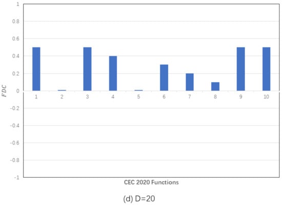
Figure 4.
FDC of CEC 2020 functions on different dimensions.
From Equation (12), we know that when the fitness value decreases as the distance from the global optimal value (for the minimization problem), the FDC value should ideally be close to 1. Once we have chosen FDC as a measure of the complexity of the optimization problem, the question becomes how to properly incorporate it into the algorithm. We introduce the concept of correlation distance,
Then . When , the optimization problem presents an obvious convex feature to some extent, and it becomes increasingly complex with the increase of . So,
is set to 0.5 so that will not be larger than 1. Through ATSP, we establish a simple linear relationship between the complexity of the optimization problem and the algorithm stage division. The algorithm can enter the exploitation stage earlier for simple unimodal problems, and otherwise, the exploration stage can be appropriately extended to find the global optimal solution as possible.
4.4. Parameter Self-Adaptation
The successful performance of the DE algorithm largely depends on the selection of the scaling factor and crossover rate [], which play a crucial role in its effectiveness, efficiency, and robustness. The mainstream method is to make the parameters adapt to different problems while iterating. A parameter-adaptive method based on the historical memory and fitness improvement weight showed good results [,,], but this may increase the risk of the population falling into a local optimum [], and the correlation between and does not get enough attention. Therefore, we adopt another parameter-adaptive method [].
The adaptive process starts with the parameter setting pool, , and probability pool, . We select (F, CR) for the initial parameter pool as [(0.1, 0.2), (0.5, 0.9), (1.0, 0.1), (1.0, 0.9)], and contains the selection probability for each pair of parameters, so each individual will select parameter pairs according to the probability . The adaptive process starts from , and adjusts the selection probability based on the performance of each pair of parameters:
where is the sum of fitness improvements corresponding to each pair of parameters, is the individual corresponding to each pair of parameters, and and are post- and pre-evolutionary individuals, respectively. From this, we can get the improvement rate corresponding to each pair of parameters,
where 0.05 is the minimum probability required for each pair of parameters. The corresponding can be obtained from as
where is the learning rate, which can be used to obtain knowledge from the performance of each group of parameters of the previous generation, so as to better guide parameter adaptation.
4.5. Complete Procedure of the Proposed TS-MSCDE
Based on the HTSDS and ATSP described above, we now present the complete steps of TS-MSCDE.
- (1)
- Initialization: The initialization of the proposed algorithm differs from classical DE, it uses LHD [] instead of randomly initializing the population, and then calculates the corresponding threshold of stage division according to ATSP.
- (2)
- Mutation: According to the preset threshold and the calculated threshold , the population was mutated by HTSDS.
- (3)
- Crossover: We use the same binomial crossover as the classic DE.
- (4)
- Selection: The same greedy selection strategy as the classic DE is adopted, that is, individuals with low fitness value enter the next iteration.
The pseudo-code of TS-MSCDE is expressed in Algorithm 1.
| Algorithm 1 Pseudo-Code for the TS-MSCDE |
|
4.6. Complexity Analysis
The complexity of the classical DE is , Where is the maximum number of iterations, is the population size, and is the problem dimension. Compared with the classical DE, the extra computation of TS-MSCDE is mainly reflected in HTSDS, ATSP, and PR_POOL calculation.
In HTSDS (see lines 17 to 27 of Algorithm 1), the main operations include population sorting to classify superior and inferior population, and then select the corresponding mutation strategy. The complexity of the sorting operator is , so we can see that the increased complexity in HTSDS is .
The ATSP (see lines 1 to 8 of Algorithm 1) mainly consists of LHD initialization and FDC calculation. The complexity corresponding to LHD is , and the complexity corresponding to FDC is , so the complexity increased by ATSP is .
The parameter adaption procedure (see line 36 to 37 of Algorithm 1) mainly consists of recalculation of the fitness value improvement rate, which increased the complexity by .
Considering the complexity of the classical DE, the complexity of the whole TS-MSCDE is , so it can be concluded that the proposed algorithm keeps the computational efficiency in time compared with the classical DE.
5. Experiments and Comparisons
In this section, the computational results of the proposed algorithm are discussed along with other state-of-the-art algorithms. First, the characteristics of , , , , and HTSDS were compared on the CEC2017 benchmark set []. Second, we validated the relevant effects of ATSP. Finally, an overall performance comparison between TS-MSCDE and advanced DE variants was conducted on the CEC2020 benchmark set []. All simulations were performed on an Intel Core i7 processor mated to a 3.4GHz CPU and 16 GB RAM.
5.1. Validation and Discussion of Classical Mutation Strategies and HTSDS
Although the characteristics of , , and have been described [], comparison with is rarely mentioned. Therefore, we compare the convergence rates of the four mutation strategies and the proposed HTSDS on typical optimization problems.
CEC2017 [], as used in this paper, contains 30 optimization functions in four categories: unimodal (F1–F3), simple multimodal (F4–F10), hybrid (F11–F20), and composition (F21–F30). This benchmark set has been used to evaluate the effectiveness of many algorithms in single-objective numerical optimization.
We chose four functions with distinct features: F1, F7, F20, and F25 (see CEC2017 for features of optimization functions). Under the classical DE framework, the initial control parameters were set as . Parameters for HTSDS were set as . We abbreviate , , and as , , , and , respectively.
Convergence curves are shown in Figure 5. achieved the top convergence speed among the four optimization functions, as expected, which is particularly important for unimodal function F1 (Figure 5a), and fell into a local optimum earliest for multimodal function F7 (Figure 5b). converged relatively slowly, especially when the difference vector size became small as iteration continued. It should be pointed out that HTSDS focuses on full exploration in the early stage, with convergence speed slower than or equal to , while in the later stage, it focuses on accelerating convergence, and the convergence speed was significantly improved. In Figure 5d, F25 (the recognized global optimal is difficult to find), the curve dropped to the lowest among all mutation strategies, which means a better solution was found in a limited number of iterations.
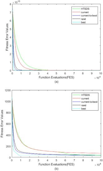
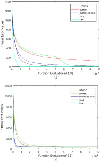
Figure 5.
Convergence curves of DEs with different mutation strategies on four 10-D CEC2017 benchmark functions: (a) F1; (b) F7; (c) F20; (d) F25.
We further discuss the characteristics of HTSDS and the other four mutation strategies, using the same settings. Because some complex problems are difficult to optimize, we add a new comparison algorithm HTSDS*, where * denotes . To reduce errors due to randomness, each algorithm was executed for 51 runs independently, with results of , as shown in Table A1, which includes the mean value (Mean) and standard deviation (Std.Dev) of the error value , with representing the global optimal value. The table gives the rank of the mean value of each algorithm for each test function. The “+”, “−”, and “=“ signs at the end of the table indicate that HTSDS* is respectively better than, equal to, or worse than other comparison algorithms.
It is not difficult to see from Table A1, when , several global optima of F1–F4 could be found for most mutation strategies. Owing to slow convergence in the late stage of , no global optima of a function could be found. From F5, ranked relatively lowly among the six algorithms because it was easily trapped in local optima. Although achieved better results on functions F1–F3, it performed poorly on F30 due to its poor robustness, and , which had similar convergence, had a more balanced performance on all functions. Most importantly, when computing resources were not added, HTSDS had average performance, but ranked relatively highly on F21–F30. After adding computing resources, HTSDS* achieved outstanding performance. HTSDS* was first on 29 functions. Compared with the other five algorithms, HTSDS* was also superior on more than 20 functions. It can be concluded that HTSDS can give full play to its effect when computing resources are sufficient.
5.2. Verifying Validity of ATSP
We saw in Section 5.1 that HTSDS accelerated later convergence compared with . However, the stage partition parameter may be too large for unimodal functions and too small for some multimodal functions. Therefore, we use the previous algorithm settings to further discuss the effectiveness of ATSP.
We set and for ATSP. For comprehensive verification, is set to , , for HTSDS-3 and HTSDS+ATSP-3, HTSDS-2 and HTSDS+ATSP-2, HTSDS-1 and HTSDS+ATSP-1, respectively. We add a new comparison item, avgFEs, in Table A2 to represent the average required FEs when the algorithm reaches the optimal condition. The global optimum is not found when avgFEs is 0.
With respect to the simple functions, i.e., F1-F4, all algorithms accurately found the global optimum in each run, and HTSDS+ATSP-3 are all smaller than HTSDS-3 in terms of avgFEs; that is, the convergence speed is faster. On complex functions F5–F30, HTSDS+ATSP-3 did not deteriorate because of ATSP. Instead, avgFEs were increased to further improve the accuracy of solutions on functions like F19 and F22. From comparison results of Table A2, HTSDS+ATSP-3 achieved better results than HTSDS-3 on 13 functions with the same computing resources. Moreover, with the reduction of computing resources, the effectiveness of ATSP diminishes considering the overall performance on all functions. We can conclude that ATSP has better adaptability than fixed parameters with relatively sufficient computing resources.
5.3. Comparison against State-of-the-Art Algorithms
It can be inferred from the previous experiments that, the mutation operator adopted by TS-MSCDE requires relatively sufficient computing resources. To verify whether TS-MSCDE performs comparably to other advanced algorithms under such conditions, we introduce the CEC2020 benchmark set []. Different from such sets as CEC2017, CEC2020 simplifies the test function set, leaving the most representative 10 optimization functions. Besides, in previous CEC competitions, the maximum allowed number of function evaluations ()—unlike problem complexity—did not scale exponentially with dimension. To address this disparity, CEC2020 significantly increases the for 10 scalable benchmark problems beyond their prior contest limits, with the goal of determining the extent to which this extra time translates into improved solution accuracy.
We set ; ; ; and . Several currently popular DE variants were chosen for comparison with TS-MSCDE, including algorithms ranked relatively high on CEC2020, and executed each algorithm 30 runs independently. These algorithms are:
- (1)
- SHADE: An efficient DE variant using a mutation strategy. SHADE has been widely studied and used for comparison [].
- (2)
- LSHADE: Based on SHADE, the linear population decline mechanism is adopted, which significantly improves performance. This is a widely used DE variant [].
- (3)
- j2020: This algorithm uses a crowding mechanism and a strategy to select the mutant vector from two subpopulations. The algorithm won third place in the CEC2020 numerical optimization competition [].
- (4)
- AGSK: This new algorithm derived from human knowledge sharing won second place in the CEC2020 numerical optimization competition [].
- (5)
- MODE: A hybrid algorithm with three differential mutation strategies and linear sequence programming. It was awarded first place in the CEC2020 numerical optimization competition [].
Table A3 lists the performance of the six algorithms on F1–F10 when . TS-MSCDE found the global optimum on F1, F5, F6, F7, and F8; IMODE found the global optimum on F9; and the other four algorithms found fewer global optima. The global optimum for F10 is generally acknowledged to be difficult to find, while TS-MSCDE has achieved outstanding performance. Overall, TS-MSCDE ranked first among all six optimization functions, IMODE ranked first among all eight functions, and the other four algorithms lagged behind.
Table A4 shows the results when . Different from , with the increase in dimension, the ability of all algorithms to find the global optimum in a stable manner decreases. Nevertheless, TS-MSCDE achieved first place in F1, F3, F8, and F10, while IMODE achieved first place in F1, F4, F6, F7, and F9. It is worth mentioning that j2020 achieved first place in F1, F2, and F5. The performance of the other three algorithms is relatively indifferent, and the ranking of the three algorithms on each function is lower.
Table A5 shows the results when . All six algorithms on F1 could still find the global optimum stably in 30 runs. TS-MSCDE ranked first on F3, F9, and F10, and still won the average by a large margin, while IMODE ranked first among all algorithms on F4, F7, and F8. Generally speaking, the performance of TS-MSCDE and IMODE was close, and the other four algorithms lagged behind.
Table A6 shows the results when . The complexity of F9 and F10 has multiplied. Experiments showed that many algorithms fall easily into local optima on the two optimization functions. TS-MSCDE still achieved outstanding results on F10, and showed the same results as IMODE on F9. TS-MSCDE had a certain probability of finding the global optimum on F3 and F8. From the final results, TS-MSCDE and IMODE ranked first among five optimization functions, but IMODE ranked slightly higher than TS-MSCDE overall.
From Table A3, Table A4, Table A5 and Table A6, it can be seen that TS-MSCDE and IMODE performed closely to each other on CEC2020, with results exceeding those of the other four algorithms. In addition to numerical comparisons, we statistically compare solution quality. In Table 1, the Wilcoxon signed-rank test (significance level , R+ is the sum of ranks for the problems in which the first algorithm outperformed the second, and R- is the sum of ranks for the opposite []) is used to compare the results between the proposed algorithm and its competitors. From to , the p-value obtained by TS-MSCDE in five rounds of comparison was less than 0.05, which indicates a big difference between TS-MSCDE and the other algorithms. We also find that TS-MSCDE won 16 rounds of comparisons in terms of the value of R+ and R−, which also reflects that TS-MSCDE achieved more promising results. We can come to the same conclusion from Table A3 to Table A6.

Table 1.
Wilcoxon test between TS-MSCDE and other algorithms using CEC2020 for D = 5, 10, 15, and 20.
In Table 2, the Friedman test, a widely used nonparametric test in the EA community, is used to validate the performance of the algorithms based on the mean value of 30 independent runs. It is not difficult to find that the p-values from to calculated by the Friedman test are all less than 0.05. Therefore, it can be concluded that there are significant differences in the performance of the comparison algorithms on the corresponding dimensions. From to , TS-MSCDE ranked first; was significantly better than AGSK, J2020, LSHADE, and SHADE; and slightly better than IMODE. On , the performance of TS-MSCDE declined to third, and was worse than IMODE and AGSK. Therefore, from the overall rank, TS-MSCDE ranked first with a slight advantage, while IMODE ranked second. The difference between the performances of the two algorithms was small, and both significantly exceeded the other four algorithms.
Table 2.
Average ranks for all algorithms across all problems and dimensions using CEC2020.
5.4. Sensitivity Analysis of Population Partition Parameter
In the above experiments, we verified the proposed HTSDS, ATSP, and TS-MSCDE in the benchmark function. In HTSDS, we set the population partition parameter to divide the population into two subpopulations. In this section, we will further discuss whether TS-MSCDE is sensitive to the change of .
First, we set as a sequence from 0.1 to 0.9 with step size 0.1. At the same time, for intuitive statistics, we introduced the cumulative rank normalization formula:
where , represents the function numbers in CEC2020, represents the rank of the mean value of TS-MSCDE in a dimension corresponding to . From Equation (19), the rank performance of the algorithm under different values in different dimensions can be obtained as Figure 6. From the figure, we can see that the rank performance of from 0.3 to 0.7 is relatively stable on , and the performance is poor beyond that. The performance of TS-MSCDE may fluctuate slightly between and , but the general trend is that after is greater than 0.5, the performance will gradually deteriorate, while before is smaller than 0.5, the performance is different. We can analysis the reasons behind, when is small, it means inferior subpopulation is larger. Connected with the description in Section 4.2, most individuals are maintaining population diversity, and a small number of individuals focus on local search. It may cause rapid convergence and frequent stagnation for superior population. Therefore, it may lead to unstable optimization results and slow convergence. When is large, it is obvious that the inferior population is small, which leads to the difficulty in maintaining population diversity and finding the region where the global optimal is located. The performance of the algorithm gradually deteriorates with the increase of . In summary, considering the optimization accuracy and convergence speed of the algorithm, is set as 0.5.
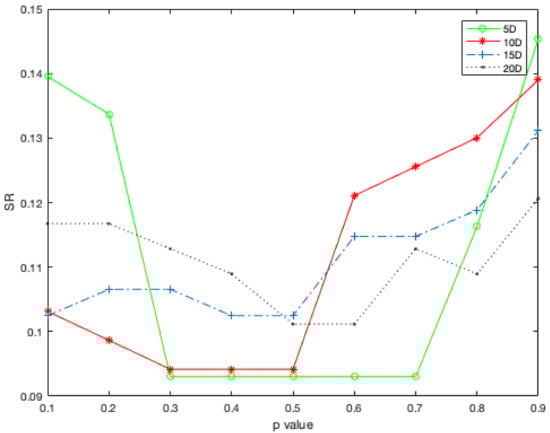
Figure 6.
Relationship between average ranks and value for four different dimensions on 10 problems from CEC 2020.
5.5. TS-MSCDE on Real-World Optimization Problems
In previous sections, we have applied TS-MSCDE to CEC2020 to prove that the algorithm can achieve excellent results under sufficient computing resources. To further extend the practical implications of the conducted research, four real-world optimization problems in CEC 2011 test suite [] are selected to judge the characteristics of the TS-MSCDE. The first real-world problem (F1) is an application to parameter estimation for frequency-modulated sound waves, which is the Problem no. 1 in CEC 2011. The second real-world problem (F2) is an application to spread spectrum radar poly-phase code design, which is the Problem no. 7 in CEC 2011. For the third real-world problem (F3), we select the 12th problem in CEC 2011, which is the so-called “Messenger” spacecraft trajectory optimization problem. Finally, the fourth real-world problem (F4) is selected from the 13th problem in CEC 2011, which defines the “Cassini 2” spacecraft trajectory optimization problem. To ensure the effectiveness of TS-MSCDE, we set for F1-F4 base on their problem dimension, other settings are consistent with Section 5.3.
As shown in Table 3, TS-MSCDE can achieve excellent results on four real-world optimization problems. It is worth mentioning that the four problems are typical complex multimodal problems and most algorithms are difficult to obtain satisfactory solutions.
Table 3.
Mean values comparison for real-world optimization problems.
6. Conclusions and Future Work
There are numerous complex optimization problems in the real world, which are difficult to obtain satisfactory solutions. When computing resources are sufficient, our first choice is to make full use of them to improve the quality of solutions. In this paper, we propose a two-stage differential evolution algorithm with mutation strategy combination (TS-MSCDE) focusing on solving this problem.
TS-MSCDE contains two search stages adaptively partitioned by ATSP and assigns different mutation strategies to superior and inferior individuals with HTSDS, so as to realize symmetrically decoupling of exploration and exploitation. Experiments were conducted on the CEC2017, CEC2020 and CEC2011 benchmark sets. From CEC2017, we can see that HTSDS+ATSP could achieve outstanding performance with sufficient computing resources. Given the curse of dimensionality, computing resources should grow exponentially with dimensions. Therefore, we selected classic DE variants SHADE and LSHADE together with IMODE, J2020, and AGSK (the top three algorithms on CEC2020) for comparative experiments. The Friedman test and the Wilcoxon test were used to analyze the performance of the algorithms. Further, four real-world optimization problems from CEC2011 are selected to verify the efficiency of TS-MSCDE. The results show that TS-MSCDE can tackle extremely difficult problems when computing resources are sufficient.
While TS-MSCDE exhibits a number of desirable characteristics, more study is required. Although HTSDS and ATSP have greatly accelerated the convergence of TS-MSCDE, the problem of slow convergence has not been completely solved. This problem occurs in some complex optimization problems with the increase of dimensions. Therefore, Future work will also focus on how to further improve the performance of TS-MSCDE under the condition of limited computing resources. Moreover, more application scenarios are worth exploring to demonstrate TS-MSCDE’s practical significance.
Author Contributions
Conceptualization: X.S., D.W. and H.K.; Data curation, X.S. and D.W.; Formal analysis, Y.S.; Investigation, Q.C. All authors have read and agreed to the published version of the manuscript.
Funding
No funding for this research.
Institutional Review Board Statement
Not applicable.
Informed Consent Statement
Not applicable.
Data Availability Statement
Data sharing is not applicable to this article.
Conflicts of Interest
We certify that we have no affiliations with or involvement in any organization or entity with any financial interest or non-financial interest in the subject matter or materials discussed in this manuscript.
Appendix A
Table A1.
Comparison results of mutation strategy on CEC2017 test suite (D = 10).
Table A1.
Comparison results of mutation strategy on CEC2017 test suite (D = 10).
| HTSDS* | HTSDS | ||||||
|---|---|---|---|---|---|---|---|
| F1 | Mean | 0.00E+00 | 0.00E+00 | 4.54E+04 | 0.00E+00 | 3.30E−03 | 0.00E+00 |
| Std.Dev | 0.00E+00 | 0.00E+00 | 1.07E+04 | 0.00E+00 | 2.06E−03 | 0.00E+00 | |
| rank | 1 | 1 | 6 | 1 | 5 | 1 | |
| F2 | Mean | 0.00E+00 | 0.00E+00 | 4.53E+00 | 0.00E+00 | 0.00E+00 | 0.00E+00 |
| Std.Dev | 0.00E+00 | 0.00E+00 | 4.57E+00 | 0.00E+00 | 0.00E+00 | 0.00E+00 | |
| rank | 1 | 1 | 6 | 1 | 1 | 1 | |
| F3 | Mean | 0.00E+00 | 0.00E+00 | 3.62E+02 | 0.00E+00 | 1.15E−02 | 0.00E+00 |
| Std.Dev | 0.00E+00 | 0.00E+00 | 9.98E+01 | 0.00E+00 | 1.27E−02 | 0.00E+00 | |
| rank | 1 | 1 | 6 | 1 | 5 | 1 | |
| F4 | Mean | 0.00E+00 | 6.60E−05 | 8.33E−01 | 0.00E+00 | 1.44E+00 | 7.24E−07 |
| Std.Dev | 0.00E+00 | 2.77E−04 | 3.28E−01 | 0.00E+00 | 3.78E−01 | 1.08E−06 | |
| rank | 1 | 4 | 5 | 1 | 6 | 3 | |
| F5 | Mean | 3.15E+00 | 1.05E+01 | 1.77E+01 | 1.51E+01 | 6.62E+00 | 6.46E+00 |
| Std.Dev | 1.17E+00 | 3.27E+00 | 3.06E+00 | 6.45E+00 | 2.40E+00 | 1.74E+00 | |
| rank | 1 | 4 | 6 | 5 | 3 | 2 | |
| F6 | Mean | 0.00E+00 | 1.86E−05 | 2.85E+00 | 7.91E−02 | 0.00E+00 | 0.00E+00 |
| Std.Dev | 0.00E+00 | 4.15E−05 | 7.60E−01 | 2.14E−01 | 0.00E+00 | 0.00E+00 | |
| rank | 1 | 4 | 6 | 5 | 1 | 1 | |
| F7 | Mean | 1.03E+01 | 2.31E+01 | 3.05E+01 | 2.76E+01 | 2.20E+01 | 1.85E+01 |
| Std.Dev | 2.43E+00 | 5.10E+00 | 5.08E+00 | 7.37E+00 | 2.31E+00 | 1.47E+00 | |
| rank | 1 | 4 | 6 | 5 | 3 | 2 | |
| F8 | Mean | 3.55E+00 | 1.10E+01 | 1.79E+01 | 1.76E+01 | 7.58E+00 | 6.81E+00 |
| Std.Dev | 1.42E+00 | 3.72E+00 | 3.17E+00 | 6.12E+00 | 2.22E+00 | 1.74E+00 | |
| rank | 1 | 4 | 6 | 5 | 3 | 2 | |
| F9 | Mean | 0.00E+00 | 0.00E+00 | 2.29E+01 | 3.45E−01 | 0.00E+00 | 0.00E+00 |
| Std.Dev | 0.00E+00 | 0.00E+00 | 1.05E+01 | 5.91E−01 | 0.00E+00 | 0.00E+00 | |
| rank | 1 | 1 | 6 | 5 | 1 | 1 | |
| F10 | Mean | 8.90E+01 | 3.17E+02 | 4.98E+02 | 5.22E+02 | 4.29E+02 | 4.03E+02 |
| Std.Dev | 7.39E+01 | 1.79E+02 | 1.14E+02 | 2.72E+02 | 1.06E+02 | 1.20E+02 | |
| rank | 1 | 2 | 5 | 6 | 4 | 3 | |
| F11 | Mean | 3.32E−02 | 2.37E+00 | 6.84E+00 | 1.72E+01 | 6.67E−01 | 1.47E+00 |
| Std.Dev | 1.82E−01 | 1.68E+00 | 1.51E+00 | 1.37E+01 | 6.54E−01 | 9.27E−01 | |
| rank | 1 | 4 | 5 | 6 | 2 | 3 | |
| F12 | Mean | 1.60E−01 | 3.18E+02 | 8.44E+03 | 4.41E+02 | 3.55E+02 | 2.00E+02 |
| Std.Dev | 1.52E−01 | 1.59E+02 | 3.34E+03 | 2.04E+02 | 1.19E+02 | 1.40E+02 | |
| rank | 1 | 3 | 6 | 5 | 4 | 2 | |
| F13 | Mean | 1.13E+00 | 7.16E+00 | 2.55E+01 | 2.69E+01 | 6.98E+00 | 4.98E+00 |
| Std.Dev | 6.26E−01 | 4.51E+00 | 6.31E+00 | 4.35E+01 | 2.07E+00 | 3.39E+00 | |
| rank | 1 | 4 | 5 | 6 | 3 | 2 | |
| F14 | Mean | 0.00E+00 | 3.17E+00 | 1.53E+01 | 2.61E+01 | 7.40E−01 | 6.14E+00 |
| Std.Dev | 0.00E+00 | 1.66E+00 | 3.06E+00 | 1.93E+01 | 5.49E−01 | 8.16E+00 | |
| rank | 1 | 3 | 5 | 6 | 2 | 4 | |
| F15 | Mean | 1.92E−03 | 1.65E+00 | 5.03E+00 | 9.57E+00 | 3.92E−01 | 4.95E−01 |
| Std.Dev | 2.79E−03 | 7.50E−01 | 1.18E+00 | 1.34E+01 | 3.22E−01 | 2.24E−01 | |
| rank | 1 | 4 | 5 | 6 | 2 | 3 | |
| F16 | Mean | 1.80E−01 | 2.12E+00 | 7.08E+00 | 8.02E+01 | 7.01E−01 | 1.83E+00 |
| Std.Dev | 1.57E−01 | 3.28E+00 | 2.44E+00 | 9.50E+01 | 2.96E−01 | 6.60E−01 | |
| rank | 1 | 4 | 5 | 6 | 2 | 3 | |
| F17 | Mean | 4.72E−02 | 8.90E+00 | 2.60E+01 | 4.27E+01 | 7.32E+00 | 1.16E+01 |
| Std.Dev | 1.35E−01 | 9.26E+00 | 5.34E+00 | 3.85E+01 | 1.71E+00 | 6.47E+00 | |
| rank | 1 | 3 | 5 | 6 | 2 | 4 | |
| F18 | Mean | 1.43E−03 | 6.52E+00 | 2.91E+01 | 2.69E+01 | 7.57E−01 | 6.19E+00 |
| Std.Dev | 1.65E−03 | 7.30E+00 | 2.45E+00 | 2.42E+01 | 4.67E−01 | 8.83E+00 | |
| rank | 1 | 4 | 6 | 5 | 2 | 3 | |
| F19 | Mean | 4.53E−03 | 6.94E−01 | 3.14E+00 | 3.76E+00 | 1.09E−01 | 7.78E−01 |
| Std.Dev | 8.36E−03 | 5.55E−01 | 5.00E−01 | 2.26E+00 | 8.89E−02 | 6.96E−01 | |
| rank | 1 | 3 | 5 | 6 | 2 | 4 | |
| F20 | Mean | 0.00E+00 | 6.26E−01 | 2.36E+01 | 2.13E+01 | 8.70E−09 | 5.47E+00 |
| Std.Dev | 0.00E+00 | 6.66E−01 | 4.72E+00 | 2.21E+01 | 2.65E−08 | 7.08E+00 | |
| rank | 1 | 3 | 6 | 5 | 2 | 4 | |
| F21 | Mean | 9.67E+01 | 1.01E+02 | 1.07E+02 | 1.70E+02 | 1.15E+02 | 1.19E+02 |
| Std.Dev | 1.83E+01 | 1.16E+00 | 1.44E+00 | 6.19E+01 | 3.86E+01 | 4.92E+01 | |
| rank | 1 | 2 | 3 | 6 | 4 | 5 | |
| F22 | Mean | 1.37E+00 | 3.26E+01 | 3.93E+01 | 9.35E+01 | 1.00E+02 | 9.72E+01 |
| Std.Dev | 4.30E+00 | 1.66E+01 | 8.61E+00 | 2.29E+01 | 1.48E−01 | 1.84E+01 | |
| rank | 1 | 2 | 3 | 4 | 6 | 5 | |
| F23 | Mean | 2.73E+02 | 2.90E+02 | 2.61E+02 | 3.19E+02 | 3.06E+02 | 3.07E+02 |
| Std.Dev | 9.08E+01 | 7.89E+01 | 1.12E+02 | 8.08E+00 | 2.34E+00 | 1.91E+00 | |
| rank | 2 | 3 | 1 | 6 | 4 | 5 | |
| F24 | Mean | 8.81E+01 | 1.00E+02 | 1.16E+02 | 3.07E+02 | 2.14E+02 | 2.68E+02 |
| Std.Dev | 3.12E+01 | 1.15E−13 | 1.65E+01 | 9.45E+01 | 1.24E+02 | 1.04E+02 | |
| rank | 1 | 2 | 3 | 6 | 4 | 5 | |
| F25 | Mean | 9.34E+01 | 1.60E+02 | 1.84E+02 | 4.32E+02 | 4.06E+02 | 4.16E+02 |
| Std.Dev | 2.54E+01 | 1.21E+02 | 2.98E+01 | 2.20E+01 | 1.76E+01 | 2.28E+01 | |
| rank | 1 | 2 | 3 | 6 | 4 | 5 | |
| F26 | Mean | 4.00E+01 | 1.47E+02 | 1.54E+02 | 3.41E+02 | 3.00E+02 | 3.00E+02 |
| Std.Dev | 8.14E+01 | 1.50E+02 | 9.40E+01 | 7.10E+01 | 3.75E−10 | 8.44E−14 | |
| rank | 1 | 2 | 3 | 6 | 5 | 4 | |
| F27 | Mean | 3.87E+02 | 3.89E+02 | 3.90E+02 | 3.98E+02 | 3.89E+02 | 3.90E+02 |
| Std.Dev | 6.95E−01 | 7.10E−01 | 4.73E−01 | 9.94E+00 | 9.73E−01 | 2.22E+00 | |
| rank | 1 | 2 | 5 | 6 | 3 | 4 | |
| F28 | Mean | 1.77E+02 | 2.10E+02 | 2.74E+02 | 4.09E+02 | 2.79E+02 | 3.66E+02 |
| Std.Dev | 1.30E+02 | 1.40E+02 | 9.54E+01 | 1.38E+02 | 1.08E+02 | 1.27E+02 | |
| rank | 1 | 2 | 3 | 6 | 4 | 5 | |
| F29 | Mean | 2.11E+02 | 2.47E+02 | 2.71E+02 | 2.96E+02 | 2.56E+02 | 2.49E+02 |
| Std.Dev | 2.96E+01 | 2.13E+01 | 1.67E+01 | 4.30E+01 | 4.84E+00 | 6.13E+00 | |
| rank | 1 | 2 | 5 | 6 | 4 | 3 | |
| F30 | Mean | 3.97E+02 | 8.77E+02 | 6.05E+03 | 2.47E+05 | 5.73E+02 | 1.24E+05 |
| Std.Dev | 4.91E+00 | 4.08E+02 | 5.38E+03 | 4.27E+05 | 6.77E+01 | 3.27E+05 | |
| rank | 1 | 3 | 4 | 6 | 2 | 5 | |
| (#) | Best | 29 | 4 | 1 | 4 | 3 | 5 |
| (#) | + | 26 | 29 | 26 | 27 | 25 | |
| (#) | = | 4 | 0 | 4 | 3 | 5 | |
| (#) | − | 0 | 1 | 0 | 0 | 0 |
Table A2.
Comparison effectiveness of ATSP on CEC2017 test suite (D = 10).
Table A2.
Comparison effectiveness of ATSP on CEC2017 test suite (D = 10).
| HTSDS-3 | HTSDS+ATSP-3 | HTSDS-2 | HTSDS+ATSP-2 | HTSDS-1 | HTSDS+ATSP-1 | ||
|---|---|---|---|---|---|---|---|
| F1 | Mean | 0.00E+00 | 0.00E+00 | 0.00E+00 | 0.00E+00 | 0.00E+00 | 0.00E+00 |
| Std.Dev | 0.00E+00 | 0.00E+00 | 0.00E+00 | 0.00E+00 | 0.00E+00 | 0.00E+00 | |
| avgFEs | 543,690 | 542,460 | 268,502 | 214,874 | 86,615 | 77,377 | |
| F2 | Mean | 0.00E+00 | 0.00E+00 | 0.00E+00 | 0.00E+00 | 0.00E+00 | 6.45E−02 |
| Std.Dev | 0.00E+00 | 0.00E+00 | 0.00E+00 | 0.00E+00 | 0.00E+00 | 3.59E−01 | |
| avgFEs | 110,298 | 109,758 | 110,543 | 109,736 | 60,317 | 62,501 | |
| F3 | Mean | 0.00E+00 | 0.00E+00 | 0.00E+00 | 0.00E+00 | 0.00E+00 | 0.00E+00 |
| Std.Dev | 0.00E+00 | 0.00E+00 | 0.00E+00 | 0.00E+00 | 0.00E+00 | 0.00E+00 | |
| avgFEs | 428,832 | 424,428 | 262,841 | 333,238 | 76,024 | 89,785 | |
| F4 | Mean | 0.00E+00 | 0.00E+00 | 0.00E+00 | 0.00E+00 | 2.62E−07 | 5.04E−07 |
| Std.Dev | 0.00E+00 | 0.00E+00 | 0.00E+00 | 0.00E+00 | 6.69E−07 | 1.97E−06 | |
| avgFEs | 793,938 | 791,406 | 278,692 | 246,792 | 45,842 | 61,850 | |
| F5 | Mean | 3.15E+00 | 3.22E+00 | 3.27E+00 | 3.40E+00 | 1.02E+01 | 1.09E+01 |
| Std.Dev | 1.17E+00 | 1.40E+00 | 1.78E+00 | 1.87E+00 | 3.74E+00 | 4.33E+00 | |
| avgFEs | 0 | 32,082 | 14,127 | 24,567 | 0 | 0 | |
| F6 | Mean | 0.00E+00 | 0.00E+00 | 0.00E+00 | 0.00E+00 | 2.05E−05 | 3.09E−05 |
| Std.Dev | 0.00E+00 | 0.00E+00 | 0.00E+00 | 0.00E+00 | 3.82E−05 | 9.84E−05 | |
| avgFEs | 1,032,570 | 945,540 | 306,964 | 290,781 | 6265 | 17,925 | |
| F7 | Mean | 1.03E+01 | 1.25E+01 | 1.32E+01 | 1.31E+01 | 2.27E+01 | 2.12E+01 |
| Std.Dev | 2.43E+00 | 2.60E+00 | 2.44E+00 | 1.47E+00 | 6.33E+00 | 6.03E+00 | |
| avgFEs | 0 | 0 | 0 | 0 | 0 | 0 | |
| F8 | Mean | 3.55E+00 | 3.38E+00 | 3.95E+00 | 3.59E+00 | 1.14E+01 | 1.12E+01 |
| Std.Dev | 1.42E+00 | 1.51E+00 | 1.86E+00 | 2.31E+00 | 3.87E+00 | 4.14E+00 | |
| avgFEs | 0 | 0 | 0 | 27,453 | 0 | 0 | |
| F9 | Mean | 0.00E+00 | 0.00E+00 | 0.00E+00 | 0.00E+00 | 0.00E+00 | 0.00E+00 |
| Std.Dev | 0.00E+00 | 0.00E+00 | 0.00E+00 | 0.00E+00 | 0.00E+00 | 0.00E+00 | |
| avgFEs | 946,686 | 920,790 | 269,878 | 270,755 | 80,721 | 83,009 | |
| F10 | Mean | 8.90E+01 | 8.00E+01 | 1.52E+02 | 1.63E+02 | 3.05E+02 | 3.15E+02 |
| Std.Dev | 7.39E+01 | 7.37E+01 | 6.62E+01 | 8.95E+01 | 1.43E+02 | 1.44E+02 | |
| avgFEs | 0 | 0 | 0 | 0 | 0 | 0 | |
| F11 | Mean | 3.32E−02 | 3.32E−02 | 8.02E−01 | 8.67E−01 | 2.63E+00 | 3.56E+00 |
| Std.Dev | 1.82E−01 | 1.82E−01 | 7.45E−01 | 8.02E−01 | 1.42E+00 | 2.40E+00 | |
| avgFEs | 1,000,914 | 1,167,558 | 131,806 | 127,510 | 2770 | 0 | |
| F12 | Mean | 1.60E−01 | 1.80E−01 | 6.99E+00 | 6.26E+00 | 2.54E+02 | 2.42E+02 |
| Std.Dev | 1.52E−01 | 1.79E−01 | 2.32E+01 | 2.13E+01 | 2.24E+02 | 1.50E+02 | |
| avgFEs | 463,290 | 461,988 | 70,955 | 19,510 | 0 | 0 | |
| F13 | Mean | 1.13E+00 | 1.26E+00 | 2.31E+00 | 2.18E+00 | 8.81E+00 | 8.82E+00 |
| Std.Dev | 6.26E−01 | 5.80E−01 | 1.44E+00 | 1.01E+00 | 4.01E+00 | 3.65E+00 | |
| avgFEs | 139,392 | 39,420 | 22,610 | 29,892 | 0 | 0 | |
| F14 | Mean | 0.00E+00 | 9.59E−07 | 5.78E−01 | 4.19E−01 | 3.19E+00 | 3.69E+00 |
| Std.Dev | 0.00E+00 | 5.25E−06 | 5.61E−01 | 4.98E−01 | 1.98E+00 | 2.47E+00 | |
| avgFEs | 1,018,974 | 1,109,688 | 158,284 | 205,467 | 0 | 2694 | |
| F15 | Mean | 1.92E−03 | 1.64E−03 | 5.69E−02 | 4.45E−02 | 1.39E+00 | 1.63E+00 |
| Std.Dev | 2.79E−03 | 3.16E−03 | 1.96E−01 | 1.78E−01 | 8.64E−01 | 9.54E−01 | |
| avgFEs | 0 | 0 | 0 | 0 | 0 | 0 | |
| F16 | Mean | 1.80E−01 | 8.39E−02 | 4.13E−01 | 3.95E−01 | 2.28E+00 | 1.71E+00 |
| Std.Dev | 1.57E−01 | 9.27E−02 | 2.48E−01 | 2.69E−01 | 3.74E+00 | 2.70E+00 | |
| avgFEs | 0 | 0 | 0 | 0 | 0 | 0 | |
| F17 | Mean | 4.72E−02 | 2.25E−02 | 3.80E−01 | 7.73E−01 | 6.74E+00 | 6.31E+00 |
| Std.Dev | 1.35E−01 | 7.89E−02 | 6.11E−01 | 1.12E+00 | 7.67E+00 | 7.32E+00 | |
| avgFEs | 889,356 | 1,133,622 | 73,794 | 84,246 | 0 | 0 | |
| F18 | Mean | 1.43E−03 | 1.19E−03 | 2.10E−02 | 4.66E−02 | 6.35E+00 | 6.37E+00 |
| Std.Dev | 1.65E−03 | 1.31E−03 | 3.85E−02 | 8.85E−02 | 7.65E+00 | 8.28E+00 | |
| avgFEs | 0 | 0 | 12896 | 0 | 0 | 0 | |
| F19 | Mean | 4.53E−03 | 1.94E−03 | 5.01E−03 | 2.55E−03 | 5.07E−01 | 5.35E−01 |
| Std.Dev | 8.36E−03 | 5.93E−03 | 8.64E−03 | 6.61E−03 | 5.86E−01 | 5.24E−01 | |
| avgFEs | 872,298 | 1,033,962 | 303,091 | 349,066 | 0 | 0 | |
| F20 | Mean | 0.00E+00 | 0.00E+00 | 0.00E+00 | 0.00E+00 | 4.89E−01 | 1.50E+00 |
| Std.Dev | 0.00E+00 | 0.00E+00 | 0.00E+00 | 0.00E+00 | 5.20E−01 | 1.60E+00 | |
| avgFEs | 1,013,676 | 1,241,676 | 294,892 | 338,063 | 8297 | 0 | |
| F21 | Mean | 9.67E+01 | 9.67E+01 | 9.35E+01 | 9.68E+01 | 9.10E+01 | 9.74E+01 |
| Std.Dev | 1.83E+01 | 1.83E+01 | 2.50E+01 | 1.80E+01 | 3.03E+01 | 1.81E+01 | |
| avgFEs | 33,786 | 35,448 | 18,029 | 9883 | 8030 | 3037 | |
| F22 | Mean | 1.37E+00 | 9.04E−01 | 1.34E+01 | 1.30E+01 | 3.50E+01 | 3.26E+01 |
| Std.Dev | 4.30E+00 | 3.48E+00 | 1.36E+01 | 1.28E+01 | 2.03E+01 | 2.28E+01 | |
| avgFEs | 924,984 | 1,010,778 | 129,426 | 120,629 | 0 | 0 | |
| F23 | Mean | 2.73E+02 | 2.57E+02 | 2.66E+02 | 2.70E+02 | 2.82E+02 | 2.70E+02 |
| Std.Dev | 9.08E+01 | 9.97E+01 | 1.04E+02 | 9.73E+01 | 9.38E+01 | 1.06E+02 | |
| avgFEs | 68,358 | 56,244 | 35,530 | 22,024 | 7485 | 9732 | |
| F24 | Mean | 8.81E+01 | 8.26E+01 | 8.06E+01 | 8.79E+01 | 9.12E+01 | 9.12E+01 |
| Std.Dev | 3.12E+01 | 3.57E+01 | 4.02E+01 | 3.19E+01 | 2.75E+01 | 2.77E+01 | |
| avgFEs | 68,214 | 58,242 | 53,803 | 13,726 | 2537 | 4883 | |
| F25 | Mean | 9.34E+01 | 9.67E+01 | 9.36E+01 | 1.10E+02 | 1.48E+02 | 1.61E+02 |
| Std.Dev | 2.54E+01 | 1.83E+01 | 2.50E+01 | 3.96E+01 | 1.12E+02 | 1.20E+02 | |
| avgFEs | 68,034 | 31,860 | 17,942 | 0 | 0 | 0 | |
| F26 | Mean | 4.00E+01 | 8.67E+01 | 6.45E+01 | 9.03E+01 | 1.00E+02 | 1.39E+02 |
| Std.Dev | 8.14E+01 | 1.01E+02 | 9.50E+01 | 1.01E+02 | 1.32E+02 | 1.48E+02 | |
| avgFEs | 809,232 | 720,288 | 185,928 | 185,812 | 47,630 | 46,574 | |
| F27 | Mean | 3.87E+02 | 3.87E+02 | 3.76E+02 | 3.88E+02 | 3.89E+02 | 3.89E+02 |
| Std.Dev | 6.95E−01 | 3.74E−01 | 6.95E+01 | 8.50E−01 | 2.84E−01 | 4.09E−01 | |
| avgFEs | 0 | 0 | 0 | 0 | 0 | 0 | |
| F28 | Mean | 1.77E+02 | 1.93E+02 | 1.77E+02 | 2.13E+02 | 2.42E+02 | 2.26E+02 |
| Std.Dev | 1.30E+02 | 1.36E+02 | 1.41E+02 | 1.31E+02 | 1.20E+02 | 1.29E+02 | |
| avgFEs | 235,842 | 299,442 | 88,815 | 68,499 | 15,410 | 18,726 | |
| F29 | Mean | 2.11E+02 | 2.07E+02 | 2.26E+02 | 2.18E+02 | 2.45E+02 | 2.44E+02 |
| Std.Dev | 2.96E+01 | 3.48E+01 | 2.90E+01 | 3.78E+01 | 9.74E+00 | 1.51E+01 | |
| avgFEs | 0 | 0 | 0 | 0 | 0 | 0 | |
| F30 | Mean | 3.97E+02 | 3.95E+02 | 4.78E+02 | 4.86E+02 | 1.04E+03 | 7.96E+02 |
| Std.Dev | 4.91E+00 | 8.23E−01 | 6.36E+01 | 6.82E+01 | 6.94E+02 | 2.69E+02 | |
| avgFEs | 0 | 0 | 0 | 0 | 0 | 0 | |
| (#) | Best | 17 | 22 | 20 | 17 | 19 | 14 |
| (#) | + | 8 | 13 | 16 | |||
| (#) | = | 9 | 7 | 3 | |||
| (#) | − | 13 | 10 | 11 |
Table A3.
Comparison results of solution accuracy on CEC2020 test suite (D = 5).
Table A3.
Comparison results of solution accuracy on CEC2020 test suite (D = 5).
| TS-MSCDE | SHADE | LSHADE | j2020 | AGSK | IMODE | ||
|---|---|---|---|---|---|---|---|
| F1 | Mean | 0.00E+00 | 0.00E+00 | 0.00E+00 | 0.00E+00 | 0.00E+00 | 0.00E+00 |
| Std.Dev | 0.00E+00 | 0.00E+00 | 0.00E+00 | 0.00E+00 | 0.00E+00 | 0.00E+00 | |
| rank | 1 | 1 | 1 | 1 | 1 | 1 | |
| F2 | Mean | 5.58E+00 | 1.59E+00 | 6.59E−01 | 3.23E+00 | 1.64E+01 | 8.33E−02 |
| Std.Dev | 5.29E+00 | 2.64E+00 | 1.69E+00 | 3.74E+00 | 2.58E+03 | 8.89E−02 | |
| rank | 5 | 3 | 2 | 4 | 6 | 1 | |
| F3 | Mean | 2.45E+00 | 4.97E+00 | 5.22E+00 | 3.42E+00 | 2.87E+00 | 5.15E+00 |
| Std.Dev | 2.20E+00 | 1.42E+00 | 7.86E−01 | 2.33E+00 | 2.05E+00 | 0.00E+00 | |
| rank | 1 | 4 | 6 | 3 | 2 | 5 | |
| F4 | Mean | 1.98E−02 | 7.48E−02 | 5.62E−02 | 7.68E−02 | 1.11E−01 | 0.00E+00 |
| Std.Dev | 4.30E−02 | 3.23E−02 | 3.22E−02 | 6.40E−02 | 6.05E−02 | 0.00E+00 | |
| rank | 2 | 4 | 3 | 5 | 6 | 1 | |
| F5 | Mean | 0.00E+00 | 2.08E−02 | 4.16E−02 | 1.37E−01 | 0.00E+00 | 0.00E+00 |
| Std.Dev | 0.00E+00 | 1.14E−01 | 1.58E−01 | 2.86E−01 | 0.00E+00 | 0.00E+00 | |
| rank | 1 | 4 | 5 | 6 | 1 | 1 | |
| F6 | Mean | 0.00E+00 | 2.82E−08 | 0.00E+00 | 0.00E+00 | 0.00E+00 | 0.00E+00 |
| Std.Dev | 0.00E+00 | 8.64E−08 | 0.00E+00 | 0.00E+00 | 0.00E+00 | 0.00E+00 | |
| rank | 1 | 6 | 1 | 1 | 1 | 1 | |
| F7 | Mean | 0.00E+00 | 0.00E+00 | 0.00E+00 | 0.00E+00 | 2.08E−02 | 0.00E+00 |
| Std.Dev | 0.00E+00 | 0.00E+00 | 0.00E+00 | 0.00E+00 | 1.14E−01 | 0.00E+00 | |
| rank | 1 | 1 | 1 | 1 | 6 | 1 | |
| F8 | Mean | 0.00E+00 | 0.00E+00 | 1.34E+01 | 6.28E−01 | 0.00E+00 | 0.00E+00 |
| Std.Dev | 0.00E+00 | 0.00E+00 | 3.47E+01 | 2.39E+00 | 0.00E+00 | 0.00E+00 | |
| rank | 1 | 1 | 6 | 5 | 1 | 1 | |
| F9 | Mean | 6.67E+00 | 1.00E+02 | 1.07E+02 | 2.05E+01 | 3.33E+01 | 0.00E+00 |
| Std.Dev | 2.54E+01 | 0.00E+00 | 4.50E+01 | 3.75E+01 | 4.79E+01 | 0.00E+00 | |
| rank | 2 | 5 | 6 | 3 | 4 | 1 | |
| F10 | Mean | 6.67E+01 | 3.39E+02 | 3.39E+02 | 1.26E+02 | 2.25E+02 | 2.44E+02 |
| Std.Dev | 4.79E+01 | 1.80E+01 | 1.80E+01 | 9.03E+01 | 1.32E+04 | 1.36E+05 | |
| rank | 1 | 5 | 5 | 2 | 3 | 4 | |
| (#) | Best | 7 | 3 | 3 | 3 | 4 | 8 |
| (#) | + | 6 | 6 | 6 | 6 | 2 | |
| (#) | = | 3 | 3 | 3 | 4 | 5 | |
| (#) | − | 1 | 1 | 1 | 0 | 3 |
Table A4.
Comparison results of solution accuracy on CEC2020 test suite (D = 10).
Table A4.
Comparison results of solution accuracy on CEC2020 test suite (D = 10).
| TS-MSCDE | SHADE | LSHADE | j2020 | AGSK | IMODE | ||
|---|---|---|---|---|---|---|---|
| F1 | Mean | 0.00E+00 | 0.00E+00 | 0.00E+00 | 0.00E+00 | 0.00E+00 | 0.00E+00 |
| Std.Dev | 0.00E+00 | 0.00E+00 | 0.00E+00 | 0.00E+00 | 0.00E+00 | 0.00E+00 | |
| rank | 1 | 1 | 1 | 1 | 1 | 1 | |
| F2 | Mean | 7.56E+01 | 9.64E+00 | 7.75E+00 | 2.58E+00 | 2.84E+01 | 4.20E+00 |
| Std.Dev | 6.18E+01 | 2.16E+01 | 4.73E+00 | 3.54E+00 | 3.21E+01 | 3.70E+00 | |
| rank | 6 | 4 | 3 | 1 | 5 | 2 | |
| F3 | Mean | 1.01E+01 | 1.66E+01 | 1.20E+01 | 1.05E+01 | 9.93E+02 | 1.21E+01 |
| Std.Dev | 3.81E+00 | 5.03E−01 | 5.97E−01 | 1.66E+00 | 4.26E+00 | 7.83E−01 | |
| rank | 1 | 5 | 3 | 2 | 6 | 4 | |
| F4 | Mean | 1.72E−02 | 2.55E−01 | 1.45E−01 | 1.39E−01 | 5.83E−02 | 0.00E+00 |
| Std.Dev | 2.84E−02 | 2.51E−02 | 1.84E−02 | 7.72E−02 | 3.11E−02 | 0.00E+00 | |
| rank | 2 | 6 | 5 | 4 | 3 | 1 | |
| F5 | Mean | 2.50E−01 | 1.99E+00 | 2.50E−01 | 1.48E−01 | 3.18E−01 | 3.88E−01 |
| Std.Dev | 1.76E−01 | 3.92E+00 | 1.27E−01 | 1.37E−01 | 3.06E−01 | 3.83E−01 | |
| rank | 3 | 6 | 2 | 1 | 4 | 5 | |
| F6 | Mean | 1.21E−01 | 2.17E−01 | 2.60E−01 | 4.78E−01 | 1.55E−01 | 9.15E−02 |
| Std.Dev | 9.69E−02 | 9.33E−02 | 1.72E−01 | 2.49E−01 | 1.17E−01 | 5.08E−02 | |
| rank | 2 | 4 | 5 | 6 | 3 | 1 | |
| F7 | Mean | 2.24E−02 | 6.94E−01 | 1.78E−01 | 6.73E−02 | 1.54E−01 | 8.54E−04 |
| Std.Dev | 6.10E−02 | 1.75E−01 | 1.95E−01 | 1.25E−01 | 1.71E−03 | 1.10E−03 | |
| rank | 2 | 6 | 5 | 3 | 4 | 1 | |
| F8 | Mean | 7.71E−01 | 1.00E+02 | 9.78E+01 | 1.54E+00 | 1.80E+01 | 2.72E+00 |
| Std.Dev | 2.93E+00 | 0.00E+00 | 1.21E+01 | 4.00E+00 | 2.38E+01 | 7.46E+00 | |
| rank | 1 | 6 | 5 | 2 | 4 | 3 | |
| F9 | Mean | 6.42E+01 | 3.83E+02 | 2.85E+02 | 8.00E+01 | 7.63E+01 | 4.11E+01 |
| Std.Dev | 4.79E+01 | 3.71E+01 | 9.39E+01 | 4.07E+01 | 4.29E+01 | 4.46E+01 | |
| rank | 2 | 6 | 5 | 4 | 3 | 1 | |
| F10 | Mean | 9.33E+01 | 4.00E+02 | 4.09E+02 | 1.40E+02 | 2.98E+02 | 3.98E+02 |
| Std.Dev | 2.54E+01 | 0.00E+00 | 1.95E+01 | 8.12E+01 | 1.43E+02 | 2.89E−13 | |
| rank | 1 | 5 | 6 | 2 | 3 | 4 | |
| (#) | Best | 4 | 1 | 1 | 3 | 1 | 5 |
| (#) | + | 8 | 7 | 7 | 8 | 4 | |
| (#) | = | 1 | 1 | 1 | 1 | 1 | |
| (#) | − | 1 | 2 | 2 | 1 | 5 |
Table A5.
Comparison results of solution accuracy on CEC2020 test suite (D = 15).
Table A5.
Comparison results of solution accuracy on CEC2020 test suite (D = 15).
| TS-MSCDE | SHADE | LSHADE | j2020 | AGSK | IMODE | ||
|---|---|---|---|---|---|---|---|
| F1 | Mean | 0.00E+00 | 0.00E+00 | 0.00E+00 | 0.00E+00 | 0.00E+00 | 0.00E+00 |
| Std.Dev | 0.00E+00 | 0.00E+00 | 0.00E+00 | 0.00E+00 | 0.00E+00 | 0.00E+00 | |
| rank | 1 | 1 | 1 | 1 | 1 | 1 | |
| F2 | Mean | 1.33E+01 | 7.56E+00 | 5.71E+00 | 5.72E−02 | 1.85E+01 | 3.14E+00 |
| Std.Dev | 9.56E+00 | 6.91E+00 | 4.47E+00 | 4.32E−02 | 1.46E+01 | 3.22E+00 | |
| rank | 5 | 4 | 3 | 1 | 6 | 2 | |
| F3 | Mean | 1.73E+00 | 1.65E+01 | 1.67E+01 | 6.78E+00 | 1.42E+01 | 1.61E+01 |
| Std.Dev | 1.69E+00 | 5.08E−01 | 5.82E−01 | 7.82E+00 | 4.27E+00 | 3.12E−01 | |
| rank | 1 | 5 | 6 | 2 | 3 | 4 | |
| F4 | Mean | 7.22E−02 | 2.61E−01 | 2.30E−01 | 1.99E−01 | 1.42E−01 | 0.00E+00 |
| Std.Dev | 6.86E−02 | 2.95E−02 | 3.06E−02 | 7.47E−02 | 5.71E−02 | 0.00E+00 | |
| rank | 2 | 6 | 5 | 4 | 3 | 1 | |
| F5 | Mean | 1.32E+01 | 1.15E+00 | 5.68E+00 | 7.58E+00 | 6.25E+00 | 7.79E+00 |
| Std.Dev | 1.11E+01 | 1.66E+00 | 2.19E+01 | 7.69E+00 | 4.32E+00 | 3.66E+00 | |
| rank | 6 | 1 | 2 | 4 | 3 | 5 | |
| F6 | Mean | 6.84E−01 | 2.14E−01 | 1.78E−01 | 8.45E−01 | 4.02E+01 | 6.92E−01 |
| Std.Dev | 3.98E−01 | 1.32E−01 | 1.24E−01 | 2.09E+00 | 2.23E−01 | 2.52E+02 | |
| rank | 3 | 2 | 1 | 5 | 6 | 4 | |
| F7 | Mean | 5.35E−01 | 7.28E−01 | 7.04E−01 | 9.83E−01 | 2.47E+01 | 5.30E−01 |
| Std.Dev | 1.86E−01 | 1.58E−01 | 2.29E−01 | 2.03E+00 | 2.00E−01 | 2.23E−01 | |
| rank | 2 | 4 | 3 | 5 | 6 | 1 | |
| F8 | Mean | 3.16E+01 | 1.00E+02 | 1.00E+02 | 9.49E+00 | 6.85E+01 | 4.18E+00 |
| Std.Dev | 3.71E+01 | 0.00E+00 | 0.00E+00 | 2.74E+01 | 3.85E+01 | 9.61E+00 | |
| rank | 3 | 5 | 5 | 2 | 4 | 1 | |
| F9 | Mean | 9.00E+01 | 3.85E+02 | 3.90E+02 | 1.23E+02 | 9.67E+03 | 9.33E+04 |
| Std.Dev | 3.05E+01 | 2.66E+01 | 3.47E−01 | 5.68E+01 | 1.83E+01 | 2.54E+04 | |
| rank | 1 | 3 | 4 | 2 | 5 | 6 | |
| F10 | Mean | 1.07E+02 | 4.00E+02 | 4.00E+02 | 3.90E+02 | 4.00E+02 | 4.00E+02 |
| Std.Dev | 2.54E+01 | 0.00E+00 | 0.00E+00 | 5.48E+01 | 2.60E−13 | 0.00E+00 | |
| rank | 1 | 3 | 3 | 2 | 3 | 3 | |
| (#) | Best | 4 | 2 | 2 | 2 | 1 | 4 |
| (#) | + | 6 | 6 | 6 | 8 | 4 | |
| (#) | = | 1 | 1 | 1 | 1 | 1 | |
| (#) | − | 3 | 3 | 3 | 1 | 5 |
Table A6.
Comparison results of solution accuracy on CEC2020 test suite (D = 20).
Table A6.
Comparison results of solution accuracy on CEC2020 test suite (D = 20).
| TS-MSCDE | SHADE | LSHADE | j2020 | AGSK | IMODE | ||
|---|---|---|---|---|---|---|---|
| F1 | Mean | 0.00E+00 | 0.00E+00 | 0.00E+00 | 0.00E+00 | 0.00E+00 | 0.00E+00 |
| Std.Dev | 0.00E+00 | 0.00E+00 | 0.00E+00 | 0.00E+00 | 0.00E+00 | 0.00E+00 | |
| rank | 1 | 1 | 1 | 1 | 1 | 1 | |
| F2 | Mean | 3.43E+00 | 2.81E+00 | 2.10E+00 | 2.60E−02 | 9.68E−01 | 5.13E−01 |
| Std.Dev | 2.53E+00 | 1.61E+00 | 1.65E+00 | 2.47E−02 | 1.23E+00 | 7.13E−01 | |
| rank | 6 | 5 | 4 | 1 | 3 | 2 | |
| F3 | Mean | 1.67E+00 | 2.08E+01 | 2.08E+01 | 1.44E+01 | 2.04E+01 | 2.05E+01 |
| Std.Dev | 3.67E+00 | 5.93E−01 | 5.13E−01 | 9.29E+00 | 0.00E+00 | 1.26E−01 | |
| rank | 1 | 6 | 5 | 2 | 3 | 4 | |
| F4 | Mean | 2.22E−01 | 3.55E−01 | 3.20E−01 | 1.80E−01 | 1.45E−01 | 0.00E+00 |
| Std.Dev | 1.54E−01 | 3.60E−02 | 2.80E−02 | 7.84E−02 | 5.47E−02 | 0.00E+00 | |
| rank | 4 | 6 | 5 | 3 | 2 | 1 | |
| F5 | Mean | 6.00E+01 | 4.57E+01 | 4.73E+01 | 7.78E+01 | 4.50E+01 | 1.09E+01 |
| Std.Dev | 5.43E+01 | 5.80E+01 | 5.87E+01 | 5.75E+01 | 3.67E+01 | 4.33E+03 | |
| rank | 5 | 3 | 4 | 6 | 2 | 1 | |
| F6 | Mean | 1.72E−01 | 3.84E−01 | 3.50E−01 | 1.92E−01 | 1.68E−01 | 3.02E−01 |
| Std.Dev | 9.61E−02 | 8.63E−02 | 7.73E−02 | 1.01E−01 | 4.45E−02 | 8.17E−02 | |
| rank | 2 | 6 | 5 | 3 | 1 | 4 | |
| F7 | Mean | 7.01E+00 | 8.14E−01 | 1.11E+00 | 1.98E+00 | 6.81E−01 | 5.24E−01 |
| Std.Dev | 8.64E+00 | 1.66E−01 | 1.54E+00 | 4.02E+00 | 9.09E−01 | 1.64E−01 | |
| rank | 6 | 3 | 4 | 5 | 2 | 1 | |
| F8 | Mean | 7.53E+01 | 1.00E+02 | 1.00E+02 | 9.27E+01 | 9.92E+01 | 8.40E+01 |
| Std.Dev | 3.25E+01 | 2.05E−13 | 1.39E−13 | 2.21E+01 | 4.63E+00 | 1.89E+01 | |
| rank | 1 | 5 | 5 | 3 | 4 | 2 | |
| F9 | Mean | 9.67E+01 | 4.03E+02 | 4.03E+02 | 3.39E+02 | 1.00E+02 | 9.67E+01 |
| Std.Dev | 1.83E+01 | 9.30E−01 | 9.93E−01 | 2.76E+01 | 8.30E−14 | 1.83E+01 | |
| rank | 1 | 6 | 5 | 4 | 3 | 1 | |
| F10 | Mean | 2.73E+02 | 4.14E+02 | 4.14E+02 | 3.99E+02 | 3.99E+02 | 4.00E+02 |
| Std.Dev | 1.46E+02 | 7.33E−03 | 1.53E−02 | 4.02E−02 | 1.59E−02 | 6.18E−01 | |
| rank | 1 | 5 | 6 | 3 | 2 | 4 | |
| (#) | Best | 5 | 1 | 1 | 2 | 2 | 5 |
| (#) | + | 6 | 6 | 6 | 4 | 4 | |
| (#) | = | 1 | 1 | 1 | 1 | 2 | |
| (#) | − | 3 | 3 | 3 | 5 | 4 |
References
- Storn, R.; Price, K. Differential Evolution–A Simple and Efficient Heuristic for global Optimization over Continuous Spaces. J. Glob. Optim. 1997, 11, 341–359. [Google Scholar] [CrossRef]
- Bhadra, T.; Bandyopadhyay, S. Unsupervised feature selection using an improved version of Differential Evolution. Expert Syst. Appl. 2015, 42, 4042–4053. [Google Scholar] [CrossRef]
- Mlakar, U.; Potočnik, B.; Brest, J. A hybrid differential evolution for optimal multilevel image thresholding. Expert Syst. Appl. 2016, 65, 221–232. [Google Scholar] [CrossRef]
- PratimSarangi, P.; Sahu, A.; Panda, M. A Hybrid Differential Evolution and Back-Propagation Algorithm for Feedforward Neural Network Training. Int. J. Comput. Appl. 2013, 84, 1–9. [Google Scholar] [CrossRef]
- Toutouh, J.; Alba, E. Optimizing OLSR in VANETS with Differential Evolution: A Comprehensive Study. In Proceedings of the 3rd International Conference on Metaheuristics and Nature Inspired Computing, Male, Maldives, 4 November 2011. [Google Scholar]
- Zhan, C.; Situ, W.; Yeung, L.F.; Tsang, P.W.-M.; Yang, G. A Parameter Estimation Method for Biological Systems modelled by ODE/DDE Models Using Spline Approximation and Differential Evolution Algorithm. IEEE/ACM Trans. Comput. Biol. Bioinform. 2014, 11, 1066–1076. [Google Scholar] [CrossRef]
- Wu, G.; Mallipeddi, R.; Suganthan, P.N. Problem Definitions and Evaluation Criteria for the CEC 2017 Competition on Constrained Real-Parameter Optimization; Technical Report for National University of Defense Technology, Changsha, Hunan, China; Kyungpook National University: Daegu, Korea; Nanyang Technological University: Singapore, 2017. [Google Scholar]
- Yue, C.; Price, K.; Suganthan, P.N.; Liang, J.; Ali, M.Z.; Qu, B.; Awad, N.H.; Biswas, P.P. Problem Definitions and Evaluation Criteria For The CEC 2020 Special Session And Competition On Single Objective Bound Constrained Numerical Optimization. Computational Intelligence Laboratory, Zhengzhou University, Zhengzhou China; Technical Report; Nanyang Technological University: Singapore, 2019. [Google Scholar]
- Das, S.; Suganthan, P.N. Problem Definitions and Evaluation Criteria for CEC 2011 Competition on Testing Evolutionary Algorithms on Real World Optimization Problems. In Proceedings of the 2011 IEEE Congress on Evolutionary Computation (CEC), New Orleans, LA, USA, 5–8 June 2011. [Google Scholar]
- Ronkkonen, J.; Kukkonen, S.; Price, K.V. Real-Parameter Optimization with Differential Evolution. In Proceedings of the 2005 IEEE Congress on Evolutionary Computation (CEC), Edinburgh, UK, 2–5 September 2005. [Google Scholar]
- Wang, Y.; Cai, Z.; Zhang, Q. Enhancing the search ability of differential evolution through orthogonal crossover. Inf. Sci. 2012, 185, 153–177. [Google Scholar] [CrossRef]
- Storn, R.; Price, K. Differential Evolution with Composite Trial Vector Generation Strategies and Control Parameters. IEEE Trans. Evol. Comput. 2011, 15, 55–66. [Google Scholar]
- Elsayed, S.M.; Sarker, R.A.; Ray, T. Differential Evolution with Automatic Parameter Configuration for Solving the CEC2013 Competition On Real-Parameter Optimization. In Proceedings of the 2013 IEEE Congress on Evolutionary Computation (CEC), Turku, Finland, 16–19 April 2013. [Google Scholar]
- Das, S.; Konar, A.; Chakraborty, U.K. Two Improved Differential Evolution Schemes for Faster Global Search. In Proceedings of the 2005 IEEE Congress on Evolutionary Computation (CEC), Cawnpore, India, 10 June 2005. [Google Scholar]
- Tvrdik, J.; Polakova, R. Competitive Differential Evolution Applied to CEC 2013 Problems. In Proceedings of the 2013 IEEE Congress on Evolutionary Computation (CEC), Turku, Finland, 20–23 June 2013. [Google Scholar]
- Coelho, L.; Ayala, H.; Freire, R.Z. Population’s Variance-Based Adaptive Differential Evolution for Real Parameter Optimization. In Proceedings of the 2013 IEEE Congress on Evolutionary Computation (CEC), Turku, Finland, 20–23 June 2013. [Google Scholar]
- Qin, K.; Huang, V.L.; Suganthan, P. Differential Evolution Algorithm With Strategy Adaptation for Global Numerical Optimization. IEEE Trans. Evol. Comput. 2008, 13, 398–417. [Google Scholar] [CrossRef]
- Liu, J.; Lampinen, J. A Fuzzy Adaptive Differential Evolution Algorithm. Soft Comput. 2004, 9, 448–462. [Google Scholar] [CrossRef]
- Brest, J.; Greiner, S.; Bošković, B.; Mernik, M.; Zumer, V. Self-Adapting Control Parameters in Differential Evolution: A Comparative Study on Numerical Benchmark Problems. IEEE Trans. Evol. Comput. 2006, 10, 646–657. [Google Scholar] [CrossRef]
- Bi, X.J.; Jing, X. JADE: Self-Adaptive Differential Evolution with Fast and Reliable Convergence Performance. In Proceedings of the 2011 IEEE Congress on Evolutionary Computation (CEC), New Orleans, LA, USA, 5–8 June 2011. [Google Scholar]
- Tanabe, R.; Fukunaga, A. Success-History Based Parameter Adaptation for Differential Evolution. In Proceedings of the 2013 IEEE Congress on Evolutionary Computation (CEC), Turku, Finland, 20–23 June 2013. [Google Scholar]
- Viktorin, A.; Senkerik, R.; Pluhacek, M.; Kadavý, T.; Zamuda, A. Distance based parameter adaptation for Success-History based Differential Evolution. Swarm Evol. Comput. 2018, 50, 100462. [Google Scholar] [CrossRef]
- Zhang, H.; Sun, J.; Xu, Z. Adaptive Structural Hyper-Parameter Configuration by Q-Learning. In Proceedings of the 2020 IEEE Congress on Evolutionary Computation (CEC), Glasgow, UK, 19–24 July 2020; pp. 1–8. [Google Scholar] [CrossRef]
- Brest, J.; Maucec, M.S.; Boskovic, B. Single objective real-parameter optimization: Algorithm jSO. In Proceedings of the 2017 IEEE Congress on Evolutionary Computation (CEC), Donostia, Spain, 5–8 June 2017. [Google Scholar]
- Das, S.; Mullick, S.S.; Suganthan, P. Recent advances in differential evolution–An updated survey. Swarm Evol. Comput. 2016, 27, 1–30. [Google Scholar] [CrossRef]
- Das, S.; Suganthan, P.N. Differential Evolution: A Survey of the State-of-the-Art. IEEE Trans. Evol. Comput. 2011, 15, 4–31. [Google Scholar] [CrossRef]
- Fan, H.Y.; Lampinen, J. A Trigonometric Mutation Operation to Differential Evolution. J. Glob. Optim. 2003, 27, 105–129. [Google Scholar] [CrossRef]
- Tanabe, R.; Fukunaga, A.S. Improving the search performance of SHADE using linear population size reduction. In Proceedings of the 2014 IEEE Congress on Evolutionary Computation (CEC), Beijing, China, 6–11 July 2014; pp. 1658–1665. [Google Scholar] [CrossRef] [Green Version]
- Liang, J.J.; Qu, B.Y.; Suganthan, P.N. Problem definitions and evaluation criteria for the CEC 2014 special session and competition on single objective real-parameter numerical optimization. In Proceedings of the 2014 IEEE Congress on Evolutionary Computation (CEC), Krakow, Poland, 6–11 July 2014. [Google Scholar]
- Islam, S.M.; Das, S.; Ghosh, S.; Roy, S.; Suganthan, P. An Adaptive Differential Evolution Algorithm With Novel Mutation and Crossover Strategies for Global Numerical Optimization. IEEE Trans. Syst. Man, Cybern. Part B 2011, 42, 482–500. [Google Scholar] [CrossRef] [PubMed]
- Zhang, X.; Yuen, S.Y. A directional mutation operator for differential evolution algorithms. Appl. Soft Comput. 2015, 30, 529–548. [Google Scholar] [CrossRef]
- Cheng, J.; Pan, Z.; Liang, H.; Gao, Z.; Gao, J. Differential evolution algorithm with fitness and diversity ranking-based mutation operator. Swarm Evol. Comput. 2020, 61, 100816. [Google Scholar] [CrossRef]
- Li, Y.; Wang, S.; Yang, B. An improved differential evolution algorithm with dual mutation strategies collaboration. Expert Syst. Appl. 2020, 153, 113451. [Google Scholar] [CrossRef]
- Loshchilov, I.; Glasmachers, T.; Beyer, H.G. Limited-Memory Matrix Adaptation for Large Scale Black-box Optimization. IEEE Trans. Evol. Comput. 2017, 23, 353–358. [Google Scholar] [CrossRef]
- Wright, S. The roles of mutation, inbreeding, crossbreeding, and selection in evolution. In Proceedings of the Sixth International Congress On Genetics, Ithaca, NY, USA, 29 October 1932. [Google Scholar]
- Caraffini, F.; Neri, F.; Picinali, L. An analysis on separability for Memetic Computing automatic design. Inf. Sci. 2014, 265, 1–22. [Google Scholar] [CrossRef]
- Pitzer, E.; Affenzeller, M. A Comprehensive Survey on Fitness Landscape Analysis. Recent Adv. Intell. Eng. Syst. 2012, 378, 161–191. [Google Scholar] [CrossRef]
- Chicano, F.; Luque, G.; Alba, E. Autocorrelation measures for the quadratic assignment problem. Appl. Math. Lett. 2012, 25, 698–705. [Google Scholar] [CrossRef] [Green Version]
- Tomassini, M.; Vanneschi, L.; Collard, P.; Clergue, M. A Study of Fitness Distance Correlation as a Difficulty Measure in Genetic Programming. Evol. Comput. 2005, 13, 213–239. [Google Scholar] [CrossRef]
- Lunacek, M.; Whitley, D. The Dispersion Metric and the CMA Evolution Strategy; Association for Computing Machinery: New York, NY, USA, 2009. [Google Scholar]
- Malan, K.M.; Engelbrecht, A.P. Quantifying Ruggedness of Continuous Landscapes using Entropy. In Proceedings of the 2009 IEEE Congress on Evolutionary Computation, Trondheim, Norway, 18–21 May 2009. [Google Scholar]
- Muñoz, M.A.; Sun, Y.; Kirley, M.; Halgamuge, S. Algorithm selection for black-box continuous optimization problems: A survey on methods and challenges. Inf. Sci. 2015, 317, 224–245. [Google Scholar] [CrossRef] [Green Version]
- Takahama, T.; Sakai, S. Differential evolution with dynamic strategy and parameter selection by detecting landscape modality. In Proceedings of the 2012 IEEE Congress on Evolutionary Computation, Brisbane, QLD, Australia, 10–15 June 2012. [Google Scholar]
- Wei, L.; Li, K.; Liang, Z.; Ying, H. A Mixed Strategies Differential Evolution Based on Fitness Landscapes Features. In Proceedings of the 2017 IEEE International Conference on Computational Science and Engineering (CSE) and IEEE International Conference on Embedded and Ubiquitous Computing (EUC), Guangzhou, China, 21–24 July 2017. [Google Scholar]
- Sallam, K.; Elsayed, S.; Sarker, R.A.; Essam, D. Landscape-based adaptive operator selection mechanism for differential evolution. Inf. Sci. 2017, 418–419, 383–404. [Google Scholar] [CrossRef]
- Mohamed, A.W.; Hadi, A.A.; Jambi, K.M. Novel mutation strategy for enhancing SHADE and LSHADE algorithms for global numerical optimization. Swarm Evol. Comput. 2018, 50, 100455. [Google Scholar] [CrossRef]
- Xia, X.; Gui, L.; Zhang, Y.; Xu, X.; Yu, F.; Wu, H.; Wei, B.; He, G.; Li, Y.; Li, K. A fitness-based adaptive differential evolution algorithm. Inf. Sci. 2020, 549, 116–141. [Google Scholar] [CrossRef]
- Li, W.; Meng, X.; Huang, Y. Fitness distance correlation and mixed search strategy for differential evolution. Neurocomputing 2020, 458, 514–525. [Google Scholar] [CrossRef]
- Zt, A.; Kl, A.; Yi, W.B. Differential evolution with adaptive mutation strategy based on fitness landscape analysis. Inf. Sci. 2021, 49, 142–163. [Google Scholar]
- Ye, K.Q. Orthogonal column Latin hypercubes and their application in computer experiments. J. Am. Stat. Assoc. 1998, 93, 1430–1439. [Google Scholar] [CrossRef]
- Mohamed, A.W.; Hadi, A.A.; Mohamed, A.K.; Awad, N.H. Evaluating the Performance of Adaptive GainingSharing Knowledge Based Algorithm on CEC 2020 Benchmark Problems. In Proceedings of the 2020 IEEE Congress on Evolutionary Computation (CEC), Glasgow, UK, 9–24 July 2020. [Google Scholar]
- Brest, J.; Maucec, M.S.; Boskovic, B. Differential Evolution Algorithm for Single Objective Bound-Constrained Optimization: Algorithm j2020. In Proceedings of the 2020 IEEE Congress on Evolutionary Computation (CEC), Glasgow, UK, 9–24 July 2020; 2020. [Google Scholar]
- Sallam, K.M.; Elsayed, S.M.; Chakrabortty, R.K.; Ryan, M.J. Improved multi-operator differential evolution algorithm for solving unconstrained problems. In Proceedings of the 2020 IEEE Congress on Evolutionary Computation (CEC), Glasgow, UK, 9–24 July 2020. [Google Scholar]
- Derrac, J.; García, S.; Molina, D.; Herrera, F. A practical tutorial on the use of nonparametric statistical tests as a methodology for comparing evolutionary and swarm intelligence algorithms. Swarm Evol. Comput. 2011, 1, 3–18. [Google Scholar] [CrossRef]
Publisher’s Note: MDPI stays neutral with regard to jurisdictional claims in published maps and institutional affiliations. |
© 2021 by the authors. Licensee MDPI, Basel, Switzerland. This article is an open access article distributed under the terms and conditions of the Creative Commons Attribution (CC BY) license (https://creativecommons.org/licenses/by/4.0/).