Detection of Influential Observations in Spatial Regression Model Based on Outliers and Bad Leverage Classification

Abstract

Influential observations (IOs), which are outliers in the x direction, y direction or both, remain a problem in the classical regression model fitting. Spatial regression models have a peculiar kind of outliers because they are local in nature. Spatial regression models are also not free from the effect of influential observations. Researchers have adapted some classical regression techniques to spatial models and obtained satisfactory results. However, masking or/and swamping remains a stumbling block for such methods. In this article, we obtain a measure of spatial Studentized prediction residuals that incorporate spatial information on the dependent variable and the residuals. We propose a robust spatial diagnostic plot to classify observations into regular observations, vertical outliers, good and bad leverage points using a classification based on spatial Studentized prediction residuals and spatial diagnostic potentials, which we refer to as $ISRs-P_{osi}$ and $ESRs-P_{osi}$. Observations that fall into the vertical outliers and bad leverage points categories are referred to as IOs. Representations of some classical regression measures of diagnostic in general spatial models are presented. The commonly used diagnostic measure in spatial diagnostics, the Cook’s distance, is compared to some robust methods, $H_i^2$ (using robust and non-robust measures), and our proposed $ISRs-P_{osi}$ and $ESRs-P_{osi}$ plots. Results of our simulation study and applications to real data showed that the Cook’s distance, non-robust ${\mathrm{H}}_{\mathrm{si}1}^2$ and robust $H_{si2}^2$ were not very successful in detecting IOs. The ${\mathrm{H}}_{\mathrm{si}1}^2$ suffered from the masking effect, and the robust $H_{si2}^2$ suffered from swamping in general spatial models. Interestingly, the results showed that the proposed $ESRs-P_{osi}$ plot, followed by the $ISRs-P_{osi}$ plot, was very successful in classifying observations into the correct groups, hence correctly detecting the real IOs.

1. Introduction

Belsley et al. [1] defined an influential observation (IO) as one which, either individually or together with several other observations, has a demonstrably large impact on the calculated values of various estimates. An influential observation could be an outlier in the X-space (leverage points) or outlier in the Y-space (vertical outlier). Leverage points can be classified into good (GLPs) and bad leverage points (BLPs). Unlike BLPs, GLPs follow the pattern of the majority of the data; hence, they are not considered as IOs as they have little or no influence on the calculated values of numerous estimates [2,3]. In this connection, Rashid et al. [2] stated that IOs could be vertical outliers (VO) or BLPs. Thus, it is very crucial to identify IOs as they are responsible for misleading conclusions about the fitted regression models and various other estimates. Once the IOs are identified, there is a need to study their impact on the model and subsequent analyses. There is a handful of studies on the diagnostic of IOs in linear regression; some examples are [1,3,4,5,6,7,8,9,10,11,12]. Other articles in the literature deal with regressions with correlated residuals, e.g., [13,14,15,16,17]. However, only a few articles deal with the detection of IOs in spatial regression models; some examples include [18,19,20,21,22]. Some robust estimation methods in spatial regression are [23,24,25]. Christensen et al. [18] and Haining [19] adapted one of the diagnostic measures in [3] to detect influential observations in spatial error autoregression model. They achieved this by defining correlated errors through the spatial weight matrix and coefficient of spatial autocorrelation in the error term. They also presented the spatial Studentized prediction residuals and the spatial leverage terms that contain error terms in spatial information.

The presence of high or low attribute value in the neighbourhood of a spatial location may result in the inability to detect the true spatial outlier, or the false identification of a good observation as an outlier [26]. Hadi [27] has also noted that spatial outlier detection methods inherit the problem of masking and swamping. Masking occurs when outlying observations are incorrectly declared as inliers. Swamping on the other hand, occurs when clean observations are incorrectly classified as outliers [28]. Aggarwal [29] observed that spatial outlier breaks the spatial autocorrelation and continuity of spatial locations. Spatial autocorrelation is a systematic pattern in attribute values that are recorded in several locations on a map. Attribute values in one location that are associated with values at neighbouring locations indicate the presence of autocorrelation. Positive autocorrelation indicates similar values that are clustered together. Negative autocorrelation indicates low attribute values in the neighbourhood of high attribute values and vice-versa [30].

Robust estimation methods mostly focus on estimations that are not influenced much by the effects of outliers. Anselin [23] has extended the bootstrap estimation to mixed regressive spatial autoregressive models, where pseudo error terms are generated by sampling from the vector of error terms. The spatial structure of the data is maintained through the generation of error terms. Politis et al. [31] and Heagerty and Lumley [32] also adopted the bootstrap method on blocks of contiguous locations to generate replicates of the estimates of the asymptotic standard error of statistics. Cerioli and Riana [24] argued that a robust estimator of the spatial autocorrelation parameters did not exist based on all datasets. They proposed a forward search algorithm based on blocks of contagious spatial locations (BFS). The BFS algorithm are drawn in such a way that the blocks retain the spatial dependence structure of the original data. Yildirim [25] proposed a robust estimation method of the log-likelihood with influence function in the spatial error model. This is achieved iteratively using scoring algorithm to estimate the parameters. Though they succeeded in obtaining robust estimates, identifying spatial outliers, which is vital in spatial statistics [26], was not achieved. Popular graphical techniques to detect spatial outliers are the scatterplot [33], the Moran’s scatterplot [30] and the pockets of nonstationarity [34]. Besides being prone to the problem of masking and swamping [26], they focused mainly on spatial outliers in the Y- space only.

Diagnostic works on models that have both spatial autocorrelations in dependent variable and residual terms are missing in the literature. The problem of masking and swamping is prevalent in spatial regression model diagnostics, which may be due to the presence of vertical outliers as well as leverage points, as in the case of linear regression ([27]). This motivates us to represent the spatial Studentized prediction residuals and spatial leverage values in the general spatial model, and to adapt and extend some robust diagnostic measures of detection of outliers and IOs in linear regression, such as Hadi’s potential ($p_{oii})$, Cook’s distance ($C{D}_i)$ [3], the overall potential influence ($H_i^2$) [10], and the external (ESRs) and internal (ISRs) Studentized residuals [1,9,10], to spatial regression models in order to minimize the problem of masking and swamping in spatial models.

In this article, we propose a robust spatial diagnostic plot and adapt some diagnostic measures in the linear regression model. Representations of the diagnostic measures in the spatial regression model are obtained, with a special emphasis on the general spatial regression model (GSM) that performs autoregression on both the dependent variable and error terms.

The main objective of this study is to propose a robust spatial diagnostic plot. Other objectives are: (1) to represent the leverage values of the hat matrix of the linear regression in the GSM model; (2) to extend the ISR of the linear regression to the GSM model; (3) to extend the ESR of the linear regression to the GSM model; (4) to extend the Cook’s distance and the overall potential influence of the linear regression to the GSM model (5) to develop a method of identification of the influential observations of the GSM model by proposing a procedure of classification of the observations into regular observations, vertical outliers, good and bad leverage points, and hence IOs; (6) to evaluate the performances of the proposed methods by using simulation studies; (7) to apply the proposed methods on gasoline price data for retail sites in Sheffield, UK, COVID-19 data in Georgia, USA, and the life expectancy data from USA counties. The significance of this study is that it can contribute to the development of a method of identification of influential observations in spatial regression models.

2. Identification of Influential Observations in a Linear Regression Model

Consider a k-variable regression model:

$$\mathit{y}=\mathit{X}\mathsf{\beta }+\mathbf{\epsilon }$$

(1)

where $\mathit{y}$ is an $n\times 1$ vector of observations of dependent variables, $\mathit{X}$ is an $n\times k$ matrix of independent variables, $\mathsf{\beta }$ is a $k\times 1$ vector of unknown regression parameters, $\mathsf{\epsilon }$ is an $n\times 1$ vector of random errors with identical normal distributions, that is, $\mathsf{\epsilon }~NID\left(0,{\mathsf{\sigma }}^2\right)$.

The ordinary least squares (OLS) estimates in Equation (1) are given by:

$$\widehat{\mathsf{\beta }}={\left({\mathit{X}}^T\mathit{X}\right)}^{-1}{\mathit{X}}^T\mathit{y}$$

(2)

The vector of predicted values can be written as:

$$\widehat{\mathit{y}}=\mathit{X}\widehat{\mathsf{\beta }}=\mathit{X}{\left({\mathit{X}}^{\mathit{T}}\mathit{X}\right)}^{-\mathbf{1}}{\mathit{X}}^{\mathit{T}}\mathit{y}=\mathit{P}\mathit{y},$$

where $\mathit{P}=\mathit{X}{\left({\mathit{X}}^T\mathit{X}\right)}^{-1}{\mathit{X}}^T$ is the hat/leverage matrix. The diagonal elements of the leverage matrix are called the hat values, denoted as $p_{ii}$, and given by:

$${\mathit{p}}_{\mathit{i}\mathit{i}}={\mathit{x}}_{\mathit{i}}^{\mathit{T}}{\left({\mathit{X}}^{\mathit{T}}\mathit{X}\right)}^{-\mathbf{1}}{\mathit{x}}_{\mathit{i}}, \mathit{i}=\mathbf{1},\mathbf{2},\mathbf{\cdots },\mathit{n}.$$

The hat matrix is often used as diagnostics to identify leverage points. Leverage is the amount of influence exerted by the observed response $y_i$ on the predicted variable ${\widehat{y}}_i$. As a result, a large leverage value indicates that the observed response has a large effect on the predicted response.

Hoaglin and Welsh [3] suggested that an observation which exceeds $\frac{2k}{n}$, where $\frac{2k}{n}$ is the average value of $p_{ii}$, is considered as a leverage point, while Vellman and Welsch suggested $\frac{3k}{n}$ as a cut-off point for leverage points. Huber [7] suggested that the ranges $p_{ii}\le 0.2$, $0.2<p_{ii}\le 0.5$ and $p_{ii}>0.5$ are safe, risky and to be avoided, respectively, for leverage values.

Unfortunately, the hat matrix suffers from the masking effect. As a result, $p_{ii}$ often fails to detect high leverage points. Hadi [10] suggested a single-case-deleted measure called potentials or Hadi’s potentials. The diagonal element of a potential denoted as $p_{oii}$, is given by:

$$p_{0ii}={\mathit{x}}_i^T\left({\mathit{X}}_{\left(i\right)}^T{\mathit{X}}_{\left(i\right)}\right){\mathit{x}}_i, i=1,2,\cdots ,n$$

(3)

where $X_{\left(i\right)}$ is the matrix X with the $i^{th}$ row deleted. We can rewrite $p_{0ii}$ as a function of $p_{ii}$ as:

$$p_{0ii}=\frac{p_{ii}}{1-p_{ii}}, i=1,2,\cdots ,n.$$

The vector of the residuals, $\mathit{r}$, can be written as:

$$\mathit{r}=\mathit{y}-\widehat{\mathit{y}}=\left(\mathit{I}-\mathit{P}\right)\mathit{y}=\mathit{Q}\mathit{y},$$

The Studentized residuals (internally Studentized residuals) denoted as ISRs and R-Student residuals (externally Studentized residuals) denoted as ESRs are widely used measures for the identification of outliers (see [7]). The ISR, denoted as $t_i$, is defined as:

$$t_i=\frac{r_i}{\widehat{\sigma }\sqrt{1-p_{ii}}}$$

where $\widehat{\sigma }$ is the standard deviation of the residuals, $r_i$ and $p_{ii}$ are the $i^{th}$ residual and diagonal element of the matrix $\mathit{P}$, respectively (see [9] for details). Meanwhile, Chatterjee and Hadi [9] defined ESR denoted as $t_i^{*}$ and given by:

$$t_i^{*}=\frac{r_i}{{\widehat{\sigma }}_{\left(i\right)}\sqrt{1-p_{ii}}}$$

where ${\widehat{\sigma }}_{\left(i\right)}$ is the residuals mean square excluding the $i^{th}$ case. The ESR follows a Student’s t-distribution with $\left(n-k-1\right)$ degrees of freedom [9].

One of the most employed measures of influence in linear regression is the Cook’s distance [3]. It measures the influence on the regression coefficient estimate or the predicted values. The Cook’s distance is given by

$${\widehat{CD}}_i\left({\mathit{X}}^{\mathit{T}}\mathit{X},k{\widehat{\sigma }}^2\right)=\frac{{\left({\widehat{\mathsf{\beta }}}^{\left(-\mathit{i}\right)}-\widehat{\mathsf{\beta }}\right)}^{\mathit{T}}\left({\mathit{X}}^{\mathit{T}}\mathit{X}\right)\left({\widehat{\mathsf{\beta }}}^{\left(-\mathit{i}\right)}-\widehat{\mathsf{\beta }}\right)}{k{\widehat{\sigma }}^2},$$

(4)

where $\widehat{\mathbf{\beta }}$ is the vector of estimates of $\mathbf{\beta }$ using the full data, ${\widehat{\mathbf{\beta }}}^{\left(-\mathit{i}\right)}$ is the vector of estimates of $\beta$ with the $i^{th}$ observation of $y_i$ and $x_i$ omitted, k is the number of parameters and ${\widehat{\sigma }}^2$ is the estimate of variance. Any $i^{th}$ observation is declared influential observation (IO) if ${\widehat{CD}}_i>F\left[0.5; k, \left(n-k\right)\right]$. Meloun [12] noted that any observation in which $C{D}_i>1$ is considered as an influential observation. The Cook’s distance can also be written as [8,9]:

$${\widehat{CD}}_i\left({\mathit{X}}^{\mathit{T}}\mathit{X},k{\widehat{\sigma }}^2\right)=\frac{{\left(\widehat{\mathit{y}}-{\widehat{\mathit{y}}}_{\mathit{i}}\right)}^{\mathit{T}}\left(\widehat{\mathit{y}}-{\widehat{\mathit{y}}}_{\mathit{i}}\right)}{k{\widehat{\sigma }}^2}$$

(5)

Computing the ${\widehat{CD}}_i\left({\mathit{X}}^{\mathit{T}}\mathit{X},k{\widehat{\sigma }}^2\right)$ does not require fitting a regression equation for each of the $i^{th}$ observations and the full model; instead, Equation (3) can further be simplified as ([3,8,9]):

$${\widehat{CD}}_i\left(X^{T}X,k{\widehat{\sigma }}^2\right)=\frac{1}{k}{t}_i^2\frac{p_{ii}}{q_{ii}}$$

(6)

where $t_i=\frac{e_i}{\widehat{\sigma }\sqrt{q_{ii}}}$ is the ISR and $\frac{p_{ii}}{q_{ii}}$ $\left(q_{ii}=1-p_{ii}\right)$ is referred to as the potential [7,8,9]. Interestingly, the Cook’s distance is a measure of influence based on the potential ($\frac{p_{ii}}{q_{ii}}$) and Studentized residual ($t_i$).

Hadi [10] demonstrated the drawback of methods that are multiplicative of functions, such as the Cook’s distance [3], Andrews–Pregibon statistic [5], Cook and Weisberg statistic [8], etc. (see [10] for details), and proposed a method that is additive of the functions. Though both the multiplicative and additive methods are functions of residuals and leverage values, the former diminishes towards zero for smaller value of any of the two functions or both, while in the latter case, the measure is large if one of the two functions or both are large. He proposed a measure of overall potential influence, denoted as ${\mathit{H}}_{\mathit{i}}^{\mathbf{2}}$, and defined as follows:

$$H_i^2=\frac{k}{m}\frac{{\mathit{e}}_{\mathit{I}}^{\mathit{T}}{\left({\mathit{I}}_{\mathit{m}}-{\mathit{P}}_{\mathit{I}}\right)}^{-1}{\mathit{e}}_{\mathit{I}}}{{\mathit{e}}^{\mathit{T}}\mathit{e}-{\mathit{e}}_{\mathit{I}}^{\mathit{T}}{\mathit{e}}_{\mathit{I}}}+\frac{1}{m}tr\left({\mathit{P}}_{\mathit{I}}{\left({\mathit{I}}_{\mathit{m}}-{\mathit{P}}_{\mathit{I}}\right)}^{-1}\right),$$

(7)

with k, the number of the parameters in the model, $\mathit{I}=\left\{i_1,i_2,\cdots ,i_m\right\}$ the set of indices of observations of length m, and ${\mathit{P}}_{\mathit{I}}$ the leverage indexed by I.

For $m=1$ and $I=i$, Equation (7) simplifies to:

$$H_i^2=\frac{k}{\left(1-p_{ii}\right)}\frac{e_i^2}{\left({\mathit{e}}^{\mathit{T}}\mathit{e}-e_i^2\right)}+\frac{p_{ii}}{1-p_{ii}}=\frac{k}{\left(1-p_{ii}\right)}\frac{d_i^2}{\left(1-d_i^2\right)}+\frac{p_{ii}}{1-p_{ii}},$$

(8)

where $\sum p_{ii}=k$, $\sum d_i^2=1$, $d_i^2=\frac{e_i^2}{e^{T}e}$ is the square of the $i^{th}$ normalized residual.

Hadi [10] suggested a cut-off point for Hadi’s potential ($p_{oii} ) and$, $H_i^2$ denoted as ($l_1$) which is given as follows:

$$l_1=mean\left(p_{oi}\right)+c\sqrt{Var\left(p_{oi}\right)}$$

$$=\frac{k}{n}+c\sqrt{\frac{ns-k^2}{n\left(n-1\right)}},$$

where $c=2, 3$, $s=\sum p_{ii}$ and ${\mathit{p}}_{\mathit{o}\mathit{i}}$ is the vector of Hadi’s potential. Since both the mean and the standard deviation are easily affected by outliers, he suggested to employ such a confidence-bound type of cut-off points by replacing the mean and the standard deviation by robust estimators, namely the median and normalized median absolute deviation, respectively. The resulting cut-off point is denoted as $l_2$;

$${\mathit{l}}_{\mathbf{2}}=\mathit{M}\mathit{e}\mathit{d}\left({\mathit{p}}_{\mathit{o}\mathit{i}}\right)+\mathit{c}\mathit{M}\mathit{A}\mathit{D}\left({\mathit{p}}_{\mathit{o}\mathit{i}}\right),$$

3. Influential Observations in Spatial Regression Models

The general spatial autoregressive model (GSM) ([21,35,36]) includes the spatial lag term and spatially correlated error structure. The data generating process (DGP) of the general spatial model is given by:

$$\mathit{y}=\mathsf{\rho }{\mathit{W}}_{\mathbf{1}}\mathit{y}+\mathit{X}\mathsf{\beta }+\mathsf{\xi }, \mathsf{\xi }=\mathsf{\lambda }{\mathit{W}}_{\mathbf{2}}\mathsf{\xi }+\mathsf{\epsilon }, \mathsf{\epsilon }\sim N\left(0,{\mathsf{\sigma }}^2{\mathit{I}}_{\mathit{n}}\right),$$

(9)

where $\mathit{y}$ is an $n\times 1$ vector of dependent variables. $\mathit{X}$ is an $n\times k$ matrix of explanatory variables. ${\mathit{W}}_{\mathbf{1}}$ and ${\mathit{W}}_{\mathbf{2}}$ are $n\times n$ spatial weight matrices. ${\mathit{I}}_{\mathit{n}}$ is an $n\times n$ identity matrix. $\mathsf{\xi }$ is the spatially correlated error term, and $\epsilon$ is the random residual term. The parameter $\mathsf{\rho }$ is the coefficient of the spatially lagged dependent variables ${\mathit{W}}_{\mathbf{1}}\mathit{y}$, and $\mathsf{\lambda }$ is the coefficient of the spatially correlated errors.

The general spatial autoregressive model in Equation (9) can be rewritten as:

$$\mathit{A}\mathit{y}=\mathit{X}\mathsf{\beta } +{\mathit{B}}^{-\mathbf{1}}\mathsf{\epsilon },$$

(10)

where $\mathit{A}={\mathit{I}}_{\mathit{n}}-\mathsf{\rho }{\mathit{W}}_{\mathbf{1}}$, $\mathsf{\xi }={\mathit{B}}^{-\mathbf{1}}\mathsf{\epsilon }$, $\mathit{B}={\mathit{I}}_{\mathit{n}}-\mathsf{\lambda }{\mathit{W}}_{\mathbf{2}}$, $\mathsf{\xi }\sim N\left(0,{\mathsf{\sigma }}^2\mathit{V}\right)$, and $\mathit{V}={\left({\mathit{B}}^{\mathit{T}}\mathit{B}\right)}^{-\mathbf{1}}$. Estimation of the parameters is achieved using the maximum likelihood estimation method.

The log-likelihood function $\left(L\right)$ is given by:

$$L=-\frac{n}{2}ln\left({\mathsf{\sigma }}^2\right)+ln\left|\mathit{A}\right|+ln\left|\mathit{B}\right|-\frac{1}{2{\mathsf{\sigma }}^2}{\left(\mathit{A}\mathit{y}-\mathit{X}\mathsf{\beta }\right)}^{\mathit{T}}{\mathit{B}}^{\mathit{T}}\mathit{B}\left(\mathit{A}\mathit{y}-\mathit{X}\mathsf{\beta }\right)$$

(11)

Let $\widehat{\mathsf{\rho }},\widehat{\mathsf{\lambda }},{\widehat{\mathsf{\sigma }}}^2,\widehat{\mathsf{\beta }}$ be the maximum likelihood estimates (MLEs) of $\mathsf{\rho },\mathsf{\lambda },{\mathsf{\sigma }}^2, \mathsf{\beta }$, respectively. The MLEs are obtained iteratively using numerical methods in the maximum likelihood estimation. Anselin [35] and LeSage [36] discussed the maximum likelihood estimation procedure of the parameters.

3.1. Leverage in Spatial Regression Model

Denote the vector of parameters in Equation (11) as ${\mathsf{\beta }}_{\mathit{a}\mathit{y}}$. The estimate of ${\mathsf{\beta }}_{\mathit{a}\mathit{y}}$, ${\widehat{\mathsf{\beta }}}_{\mathit{a}\mathit{y}}$, is given by:

$${\widehat{\mathsf{\beta }}}_{\mathit{a}\mathit{y}}={\left({\mathit{X}}^{\mathit{T}}{\widehat{\mathit{V}}}^{-\mathbf{1}}\mathit{X}\right)}^{-\mathbf{1}}{\mathit{X}}^{\mathit{T}}{\widehat{\mathit{V}}}^{-\mathbf{1}}\widehat{\mathit{A}}\mathit{y}.$$

The model (11) is viewed as fitting a general linear model, $\mathit{A}\mathit{y}$ on $\mathit{X}$, that has correlated residual terms. Set $\mathit{z}=\mathit{A}\mathit{y}$, where $var\left(\mathit{A}\mathit{y}\right)={\mathsf{\sigma }}^2\mathit{V}$. Therefore,

$$\widehat{\mathit{z}}=\mathit{X}{\widehat{\mathsf{\beta }}}_{\mathit{a}\mathit{y}}=\mathit{X}{\left({\mathit{X}}^{\mathit{T}}{\widehat{\mathit{V}}}^{-\mathbf{1}}\mathit{X}\right)}^{-\mathbf{1}}{\mathit{X}}^{\mathit{T}}{\widehat{\mathit{V}}}^{-\mathbf{1}}\mathit{z}={\mathit{P}}_{\mathit{a}\mathit{y}}\mathit{z}$$

The hat matrix, in this case, is given by ${\mathit{P}}_{\mathit{a}\mathit{y}}$,

$${\mathit{P}}_{\mathit{a}\mathit{y}}=\mathit{X}{\left({\mathit{X}}^{\mathit{T}}{\widehat{\mathit{V}}}^{-\mathbf{1}}\mathit{X}\right)}^{-\mathbf{1}}{\mathit{X}}^{\mathit{T}}{\widehat{\mathit{V}}}^{-\mathbf{1}}.$$

Let ${\mathit{Q}}_{\mathit{a}\mathit{y}}={\mathit{I}}_{\mathit{n}}-{\mathit{P}}_{\mathit{a}\mathit{y}}$. Though ${\mathit{P}}_{\mathit{a}\mathit{y}}$ and ${\mathit{Q}}_{\mathit{a}\mathit{y}}$ have satisfied the idempotence property and their sum of diagonal elements equals k and $n-k$, respectively, they are not symmetric. As a result, they are not positive semi-definite, and as such, the diagonal elements of ${\mathit{P}}_{\mathit{a}\mathit{y}}$ will have negative values. The hat matrices ${\mathit{P}}_{\mathit{a}\mathit{y}}$ and ${\mathit{Q}}_{\mathit{a}\mathit{y}}$ are not symmetric, and their diagonal values do not lie between 0 and 1 (inclusive).

Martins [15] proposed a measure of leverage that is orthogonal, in the models with correlated residuals, whose diagonal values lie in the interval [0, 1], which we denote by ${\mathit{P}}_{\mathit{a}\mathit{y}}^{*}$, such that:

$${\mathit{P}}_{\mathit{a}\mathit{y}}^{*}={\widehat{\mathit{V}}}^{-\mathbf{1}}{\mathit{P}}_{\mathit{a}\mathit{y}}={\widehat{\mathit{V}}}^{-\mathbf{1}}\mathit{X}{\left({\mathit{X}}^{\mathit{T}}{\widehat{\mathit{V}}}^{-\mathbf{1}}\mathit{X}\right)}^{-\mathbf{1}}{\mathit{X}}^{\mathit{T}}{\widehat{\mathit{V}}}^{-\mathbf{1}}$$

Let ${\mathit{Q}}_{\mathit{a}\mathit{y}}^{*}={\mathit{I}}_{\mathit{n}}-{\mathit{P}}_{\mathit{a}\mathit{y}}^{*}$. ${\mathit{P}}_{\mathit{a}\mathit{y}}^{*}$ and ${\mathit{Q}}_{\mathit{a}\mathit{y}}^{*}$ are idempotent, symmetric and orthogonal with respect to $\mathit{V}$, i.e.,

• ${\mathit{P}}_{\mathit{a}\mathit{y}}^{*}\widehat{\mathit{V}}{\mathit{P}}_{\mathit{a}\mathit{y}}^{*}={\mathit{P}}_{\mathit{a}\mathit{y}}^{*}$
• ${\mathit{Q}}_{\mathit{a}\mathit{y}}^{*}\widehat{\mathit{V}}{\mathit{Q}}_{\mathit{a}\mathit{y}}^{*}={\mathit{Q}}_{\mathit{a}\mathit{y}}^{*}$
• ${\mathit{P}}_{\mathit{a}\mathit{y}}^{*}\widehat{\mathit{V}}{\mathit{Q}}_{\mathit{a}\mathit{y}}^{*}=\mathbf{0}$

Note that the sum of the diagonal elements of ${\mathit{P}}_{\mathit{a}\mathit{y}}^{*}$ and ${\mathit{Q}}_{\mathit{a}\mathit{y}}^{*}$, the leverage, does not sum to $k$ and $n-k$.

Again, consider a new set of dependent variables obtained by pre-multiplying Equation (11) by the matrix $\mathit{B}$ ($\mathit{B}$ as defined in Equation (10)) so that ${\mathit{z}}^{*}=\mathit{B}\mathit{A}\mathit{y}$. Schall and Dunne [14] defined the matrix ${\mathit{V}}^{-\mathbf{1}}$ as a singular value decomposition such that ${\mathit{V}}^{-\mathbf{1}}=\mathit{B}\mathbf{\Delta }{\mathit{B}}^{\mathit{T}}$; where $\mathit{B}$ is of the same order as ${\mathit{V}}^{-\mathbf{1}}$ and $\mathbf{\Delta }$ is a diagonal matrix. The transformation ${\mathit{z}}^{*}$ is the principal component score. Puterman [13] and Haining [19] defined it as canonical variates such that $\mathit{B}\mathit{X}\left({\mathit{X}}^{\mathit{T}}{\mathit{V}}^{-\mathbf{1}}\mathit{X}\right){\mathit{X}}^{\mathit{T}}{\mathit{B}}^{\mathit{T}}$ is positive semi-definite. By setting ${\mathit{z}}^{*}=\mathit{B}\mathit{A}\mathit{y}$, Equation (9) is rewritten in a generalized least squares (GLS) form as:

$${\mathit{z}}^{*}={\mathit{X}}^{*}{\mathsf{\beta }}_{\mathit{s}}+\mathsf{\epsilon },\mathsf{\epsilon }\sim N\left(0,{\mathsf{\sigma }}^2{\mathit{I}}_{\mathit{n}}\right)$$

(12)

where ${\mathit{X}}^{*}=\mathit{B}\mathit{X}$.

The estimate ${\widehat{\mathsf{\beta }}}_{\mathit{s}}$ of ${\mathsf{\beta }}_{\mathit{s}}$ is now given by:

$${\widehat{\mathsf{\beta }}}_{\mathit{s}}={\left({\mathit{X}}^{*}{}^{\mathit{T}}{\mathit{X}}^{*}\right)}^{-\mathbf{1}}{\mathit{X}}^{*}{}^{\mathit{T}}{\mathit{z}}^{*}$$

Thus,

$${\widehat{\mathit{z}}}^{*}={\mathit{X}}^{*}{\left({\mathit{X}}^{*}{}^{\mathit{T}}{\mathit{X}}^{*}\right)}^{-\mathbf{1}}{\mathit{X}}^{*}{}^{\mathit{T}}{\mathit{z}}^{*}$$

(13)

where, $\widehat{\mathit{A}}={\mathit{I}}_{\mathit{n}}-\widehat{\mathsf{\rho }}{\mathit{W}}_{\mathbf{1}}$ and $\widehat{\mathit{B}}={\mathit{I}}_{\mathit{n}}-\widehat{\mathsf{\lambda }}{\mathit{W}}_2$. Note that $\widehat{\mathit{y}}$ is deduced from Equation (13) as follows:

$$\widehat{\mathit{B}}\widehat{\mathit{A}}\widehat{\mathit{y}}=\widehat{\mathit{B}}\mathit{X}{\left({\mathit{X}}^{\mathit{T}}{\widehat{\mathit{B}}}^{\mathit{T}}\widehat{\mathit{B}}\mathit{X}\right)}^{-\mathbf{1}}{\mathit{X}}^{\mathit{T}}{\widehat{\mathit{B}}}^{\mathit{T}}\widehat{\mathit{B}}\widehat{\mathit{A}}\mathit{y}$$

$$\stackrel{\mathit{y}\mathit{i}\mathit{e}\mathit{l}\mathit{d}\mathit{s}}{\to }\widehat{\mathit{y}}={\widehat{\mathit{A}}}^{-\mathbf{1}}\mathit{X}{\left({\mathit{X}}^{\mathit{T}}{\widehat{\mathit{V}}}^{-\mathbf{1}}\mathit{X}\right)}^{-\mathbf{1}}{\mathit{X}}^{\mathit{T}}{\widehat{\mathit{V}}}^{-\mathbf{1}}\widehat{\mathit{A}}\mathit{y}$$

Denote the projection matrix in the transformed spatial regression model as ${\mathit{P}}_{\mathit{s}}$, then:

$${\mathit{P}}_{\mathit{s}}={\mathit{X}}^{*}{\left({\mathit{X}}^{*}{}^{\mathit{T}}{\mathit{X}}^{*}\right)}^{-\mathbf{1}}{\mathit{X}}^{*}{}^{\mathit{T}}$$

$$=\widehat{\mathit{B}}\mathit{X}{\left({\mathit{X}}^{\mathit{T}}{\widehat{\mathit{V}}}^{-\mathbf{1}}\mathit{X}\right)}^{-\mathbf{1}}{\mathit{X}}^{\mathit{T}}{\widehat{\mathit{B}}}^{\mathit{T}}, \widehat{\mathit{V}}={\left({\widehat{\mathit{B}}}^{\mathit{T}}\widehat{\mathit{B}}\right)}^{-\mathbf{1}}$$

The properties of the leverage in the transformed spatial model in Equation (13) are:

Property I: idempotent and symmetric.

Property Ia: idempotence

$${\mathit{P}}_{\mathit{s}}^{\mathbf{2}}=\widehat{\mathit{B}}\mathit{X}{\left({\mathit{X}}^{\mathit{T}}{\widehat{\mathit{V}}}^{-\mathbf{1}}\mathit{X}\right)}^{-\mathbf{1}}{\mathit{X}}^{\mathit{T}}{\widehat{\mathit{B}}}^{\mathit{T}}\widehat{\mathit{B}}\mathit{X}{\left({\mathit{X}}^{\mathit{T}}{\widehat{\mathit{V}}}^{-\mathbf{1}}\mathit{X}\right)}^{-\mathbf{1}}{\mathit{X}}^{\mathit{T}}{\widehat{\mathit{B}}}^{\mathit{T}}$$

$$=\widehat{\mathit{B}}\mathit{X}{\left({\mathit{X}}^{\mathit{T}}\widehat{\mathit{V}}\mathit{X}\right)}^{-\mathbf{1}}{\mathit{X}}^{\mathit{T}}{\widehat{\mathit{B}}}^{\mathit{T}}$$

$$={\mathit{P}}_{\mathit{s}}$$

Hence, ${\mathit{P}}_{\mathit{s}}$ is idempotent.

Property Ib: symmetric

$${\mathit{P}}_{\mathit{s}}^{\mathit{T}}={\left(\widehat{\mathit{B}}\mathit{X}{\left({\mathit{X}}^{\mathit{T}}{\widehat{\mathit{V}}}^{-\mathbf{1}}\mathit{X}\right)}^{-\mathbf{1}}{\mathit{X}}^{\mathit{T}}{\widehat{\mathit{B}}}^{\mathit{T}}\right)}^{\mathit{T}}$$

$$=\widehat{\mathit{B}}\mathit{X}{\left({\mathit{X}}^{\mathit{T}}{\widehat{\mathit{V}}}^{-\mathbf{1}}\mathit{X}\right)}^{-\mathbf{1}}{\mathit{X}}^{\mathit{T}}{\widehat{\mathit{B}}}^{\mathit{T}}$$

$$={\mathit{P}}_{\mathit{s}}$$

The matrix ${\mathit{P}}_{\mathit{s}}$ is symmetric. Therefore, ${\mathit{P}}_{\mathit{s}}$ in the transformation ${\mathit{z}}^{*}=\widehat{\mathit{B}}\widehat{\mathit{A}}\mathit{y}$ is both idempotent and symmetric.

Property II: the sum of the diagonal terms of the projection matrix is $\mathit{k}$, the number of parameters including the constant term.

$$trace\left({\mathit{P}}_{\mathit{s}}\right)=trace\left(\widehat{\mathit{B}}\mathit{X}{\left({\mathit{X}}^{\mathit{T}}{\widehat{\mathit{V}}}^{-\mathbf{1}}\mathit{X}\right)}^{-\mathbf{1}}{\mathit{X}}^{\mathit{T}}{\widehat{\mathit{B}}}^{\mathit{T}}\right)$$

$$=trace\left({\widehat{\mathit{B}}}^{\mathit{T}}\widehat{\mathit{B}}\mathit{X}{\left({\mathit{X}}^{\mathit{T}}{\widehat{\mathit{V}}}^{-\mathbf{1}}\mathit{X}\right)}^{-\mathbf{1}}{\mathit{X}}^{\mathit{T}}\right)\left(cyclic permutation of trace of matrix\right)$$

$$=trace\left({\mathit{X}}^{\mathit{T}}{\widehat{\mathit{V}}}^{-\mathbf{1}}\mathit{X}{\left({\mathit{X}}^{\mathit{T}}{\widehat{\mathit{V}}}^{-\mathbf{1}}\mathit{X}\right)}^{-\mathbf{1}}\right)\left(cyclic permutation of trace of matrix\right)$$

$$=trace\left(I_k\right)$$

$$=k,$$

where ${\mathit{I}}_{\mathit{k}}$ is an $k\times k$ identity matrix.

Therefore, ${\displaystyle \sum }_{i=\mathbf{1}}^{k}p{s}_{ii}=k$. $p{s}_{ii}$ is the $i^{th}$ diagonal element of the leverage ${\mathit{P}}_{\mathit{s}}$.

Property III: bounds on the spatial leverage.

The bound on the leverage of the classical regression is $0\le p_{ii}\le \mathbf{1}$ due to the fact that the hat matrix $\mathit{P}$ satisfies all the orthogonal properties, including symmetry. As such, it is positive semi-definite. However, the spatial leverage ${\mathit{P}}_{\mathit{a}\mathit{y}}$ is not symmetric because positive semi-definite matrix is symmetric [37,38,39]. The transformation in Equation (11) yields the projection ${\mathit{P}}_{\mathit{s}}$ that satisfies the symmetry condition.

From the idempotent property of ${\mathit{P}}_{\mathit{s}}$,

$${\mathit{P}}_{\mathit{s}}={\mathit{P}}_{\mathit{s}}^{\mathbf{2}}.$$

Equating diagonal terms of LHS and RHS, we have:

$$p{s}_{ii}=p{s}_{ii}^2+{{\displaystyle \sum }}_{j\ne i}p{s}_{ij}p{s}_{ji}, {{\displaystyle \sum }}_{j\ne i}p{s}_{ij}p{s}_{ji}\ge 0,$$

(14)

where $p{s}_{ij}$ are the off-diagonal terms. Equation (14) implies that $p{s}_{ii}\ge 0$. Therefore,

$$p{s}_{ii}\ge p{s}_{ii}^2$$

$$\stackrel{yields}{\to }p{s}_{ii}\le 1.$$

Note that ${\mathit{P}}_{\mathit{s}}$ and $Q_{\mathit{s}}$ are orthogonal:

• ${\mathit{P}}_{\mathit{s}}{\mathit{P}}_{\mathit{s}}={\mathit{P}}_{\mathit{s}}$
• $Q_{\mathit{s}}{Q}_{\mathit{s}}=Q_{\mathit{s}}$
• ${\mathit{P}}_{\mathit{s}}{Q}_{\mathit{s}}=\mathbf{0}$

The model in Equation (9) gives rise to different special spatial regressions in accordance with different restrictions. Such special spatial regression models are the spatial autoregressive-regressive model (SAR) and the spatial error model (SEM). While the former has spatial autoregression in the response variable, the latter has spatial autoregression in the model residual; model (9) (GSM) combines both features.

The spatial autoregressive-regressive model is obtained when the coefficient of the lagged spatial autoregression in the residuals of Equation (9) is zero, i.e., $\mathsf{\lambda }=0$. Thus, the SAR model is given by:

$$\mathit{y}=\mathsf{\rho }{\mathit{W}}_{\mathbf{1}}\mathit{y}+\mathit{X}\mathsf{\beta }+\mathsf{\epsilon }, \mathsf{\epsilon }\sim N\left(0,{\mathsf{\sigma }}^{\mathbf{2}}{\mathit{I}}_{\mathit{n}}\right).$$

(15)

The ${\mathit{P}}_{\mathit{s}}$ corresponding to the model in Equation (13) reduces to:

$${\mathit{P}}_{\mathit{s}}=\mathit{X}{\left({\mathit{X}}^{\mathit{T}}\mathit{X}\right)}^{-\mathbf{1}}{\mathit{X}}^{\mathit{T}},$$

with the transformation in Equation (11) simplifying to ${\mathit{z}}^{*}=\mathit{A}\mathit{y}$, since $\mathit{V}={\left({\mathit{B}}^{\mathit{T}}\mathit{B}\right)}^{-\mathbf{1}}$ and $\mathit{B}={\mathit{I}}_{\mathit{n}}$, when $\mathsf{\lambda }=0$. Clearly, the hat matrix in the SAR model preserves the features of the hat matrix in the classical regression model.

In the spatial error model (SEM), the coefficient of the spatial autoregression on the lagged dependent variable is zero, i.e., $\mathsf{\rho }=0$. This yields the model:

$$\mathit{y}=\mathit{X}\mathsf{\beta }+\mathsf{\xi }, \mathsf{\xi }=\mathsf{\lambda }{\mathit{W}}_{\mathbf{2}}\mathsf{\xi }+\mathsf{\epsilon }, \mathsf{\epsilon }\sim \mathit{N}\left(\mathbf{0},{\mathsf{\sigma }}^{\mathbf{2}}{\mathit{I}}_{\mathit{n}}\right)$$

(16)

The transformation in Equation (11) simplifies to ${\mathit{z}}^{*}=\mathit{B}\mathit{y},$ and the projection matrix remains:

$${\mathit{P}}_{\mathit{s}}=\mathit{B}\mathit{X}{\left({\mathit{X}}^{\mathit{T}}{\mathit{V}}^{-\mathbf{1}}\mathit{X}\right)}^{-\mathbf{1}}{\mathit{X}}^{\mathit{T}}{\mathit{B}}^{\mathit{T}}.$$

It can be observed that the leverage measure in the spatial regression model is dominated by the autocorrelation in the residual term.

Works on spatial regression diagnostics in the literature mainly focus on the autocorrelation in the residuals, mostly using a time series analogy [13,14,15]. Some remarkable works on the spatial regression model can be found in [18,19,21].

3.2. Influential Observations in Spatial Regression Model

The leverages ${\mathit{P}}_{\mathit{s}}$ and $Q_{\mathit{s}}$ in Equation (11) satisfy all the properties of a projection matrix, including that the sum of the diagonal terms of ${\mathit{P}}_{\mathit{s}}$ and $Q_{\mathit{s}}$ equal $\mathit{k}$ and $n - k$, respectively. It also incorporates the autocorrelation in the dependent variables, $\mathit{W}\mathit{y}$. Hence, it can be used as a diagnostic measure of leverage points in a spatial regression model.

By extending the results of linear regression to spatial regression with slight modification, the Cook’s distance in the spatial regression of Equation (13), denoted as $C{D}_{\mathit{s}i}$, can be formulated as follows:

$${\widehat{\mathit{C}\mathit{D}}}_{\mathit{s}\mathit{i}}=\frac{{\left({\widehat{\mathsf{\beta }}}_{\mathit{s}}{}^{\left(-\mathit{i}\right)}- {\widehat{\mathsf{\beta }}}_{\mathit{s}}\right)}^{\mathit{T}}\left({\mathit{X}}^{*\mathit{T}}{\mathit{X}}^{*}\right)\left({\widehat{\mathsf{\beta }}}_{\mathit{s}}{}^{\left(-\mathit{i}\right)}-{\widehat{\mathsf{\beta }}}_{\mathit{s}}\right)}{\mathit{k}{\widehat{\mathsf{\sigma }}}^{\mathbf{2}}}$$

$$=\frac{{\left({\widehat{\mathsf{\beta }}}_{\mathit{s}}{}^{\left(-\mathit{i}\right)}- {\widehat{\mathsf{\beta }}}_{\mathit{s}}\right)}^{\mathit{T}}\left({\left(\mathit{B}\mathit{X}\right)}^{\mathit{T}}\left(\mathit{B}\mathit{X}\right)\right)\left({\widehat{\mathsf{\beta }}}_{\mathit{s}}{}^{\left(-\mathit{i}\right)}- {\widehat{\mathsf{\beta }}}_{\mathit{s}}\right)}{\mathit{k}{\widehat{\mathsf{\sigma }}}^{\mathbf{2}}}$$

$$=\frac{{\left({\widehat{\mathsf{\beta }}}_{\mathit{s}}{}^{\left(-\mathit{i}\right)}- {\widehat{\mathsf{\beta }}}_{\mathit{s}}\right)}^{\mathit{T}}\left({\mathit{X}}^{\mathit{T}}{\mathit{B}}^{\mathit{T}}\mathit{B}\mathit{X}\right)\left({\widehat{\mathsf{\beta }}}_{\mathit{s}}{}^{\left(-\mathit{i}\right)}- {\widehat{\mathsf{\beta }}}_{\mathit{s}}\right)}{\mathit{k}{\widehat{\mathsf{\sigma }}}^{\mathbf{2}}}$$

$$=\frac{{\left({\widehat{\mathsf{\beta }}}_{\mathit{s}}{}^{\left(-\mathit{i}\right)}- {\widehat{\mathsf{\beta }}}_{\mathit{s}}\right)}^{\mathit{T}}\left({\mathit{X}}^{\mathit{T}}{\mathit{V}}^{-\mathbf{1}}\mathit{X}\right)\left({\widehat{\mathsf{\beta }}}_{\mathit{s}}{}^{\left(-\mathit{i}\right)}- {\widehat{\mathsf{\beta }}}_{\mathit{s}}\right)}{\mathit{k}{\widehat{\mathsf{\sigma }}}^{\mathbf{2}}},$$

where:

$${\widehat{\mathsf{\beta }}}_{\mathit{s}}{}^{\left(-\mathit{i}\right)}={\mathit{X}}_{\left(\mathit{i}\right)}{\left({\mathit{X}}_{\left(\mathit{i}\right)}^{\mathit{T}}{\widehat{\mathit{V}}}_{\left(\mathit{i},\mathit{i}\right)}^{-\mathbf{1}}{\mathit{X}}_{\left(\mathit{i}\right)}\right)}^{-\mathbf{1}}{\mathit{X}}_{\left(\mathit{i}\right)}^{\mathit{T}}{\widehat{\mathit{V}}}_{\left(\mathit{i},\mathit{i}\right)}^{-\mathbf{1}}{\widehat{\mathit{A}}}_{\left(\mathit{i},\mathit{i}\right)}{Y}_{\left(\mathit{i}\right)}.$$

${\widehat{\mathit{V}}}_{\left(\mathit{i},\mathit{i}\right)}$ and ${\widehat{\mathit{A}}}_{\left(\mathit{i},\mathit{i}\right)}$ denote $\widehat{\mathit{V}}$ and $\widehat{\mathit{A}}$ with the $i^{th}$ row and the $i^{th}$ column deleted, respectively.

The spatial Cook distance, $C{D}_{si}$, is declared large if $C{D}_{si}>0.70$ [19]. In its simplified form, the Cook’s distance in spatial regression is written as

$${\widehat{CD}}_{si}\left(X^T{V}^{-1}X,k{\widehat{\mathsf{\sigma }}}^2\right)=\frac{1}{k}{t}_{si}^2\frac{{\mathrm{p}}_{\mathrm{si}}}{{\mathrm{q}}_{\mathrm{si}}},$$

(17)

where $t_{si}$ is the spatial Studentized prediction residual (also called spatial internally Studentized residual), $p_{si}$ is the spatial leverage, which is the $i^{th}$ diagonal element of ${\mathit{P}}_{\mathit{s}}$, and $q_{si}=1-p_{si}$. Let $r_{si}=y_i-{\widehat{y}}_i$, then:

$$t_{si}=\frac{b_i^T{a}_i{r}_{si}}{\widehat{\sigma }\sqrt{q_{si}}},$$

(18)

where ${\mathit{b}}_{\mathit{i}}$ and ${\mathit{a}}_{\mathit{i}}$ are the $i^{th}$ columns of matrices $\mathit{B}$ and $\mathit{A}$, respectively. The spatial Studentized residual has a cut-off point of 2 to declare a point large [19,40].

Similarly, the spatial externally Studentized residual (ESRs), is defined as:

$$t_{\mathit{s}\mathit{i}}^{*}=\frac{r_{\mathit{s}\mathit{i}}}{{\widehat{\mathsf{\sigma }}}_{\left(\mathit{i}\right)}\sqrt{\mathbf{1}-p_{\mathit{s}\mathit{i}}}}$$

$$=t_{\mathit{s}\mathit{i}}\sqrt{\frac{n-k-\mathbf{1}}{n-k-t_{\mathit{s}\mathit{i}}^{\mathbf{2}}}}, {\widehat{\mathsf{\sigma }}}_{\left(\mathit{i}\right)}=\widehat{\mathsf{\sigma }}\left(\frac{n-k-t_{\mathit{s}\mathit{i}}}{n-k-\mathbf{1}}\right).$$

where ${\widehat{\sigma }}_{\left(i\right)}$ is the residuals mean square excluding the $i^{th}$ case. The ESRs follow a Student’s t-distribution with $\left(n-k-1\right)$ degrees of freedom. Thus, the spatial Studentized prediction residuals contain the neighbourhood information of both the dependent variable and the residual of each $r_{si}$, and the leverage ${\mathit{P}}_{\mathit{s}}$ contains the residual autocorrelation effect. The spatial potential, which is analogous to the potential in [10], is defined in Equation (19) as:

$$p_{osi}=\frac{p_{si}}{q_{si}}$$

(19)

where $q_{si}=1-p_{si}$. Let $q_{osi}=1-p_{osi}$.

We define the spatial measure of overall potential influence as

$$H_{si}^2=\frac{k}{q_{osi}}\frac{d_i^2}{\left(1-d_i^2\right)}+\frac{p_{osi}}{q_{osi}}$$

(20)

When measuring the influence of an observation in a linear regression model by using the Cook’s distance [3], the observation in question is deleted, and the model is then refitted. In a similar way, usually a group of suspected influential observations is deleted in the linear regression and admitted into the model if it is proven clean (BACON [41,42], DGRP [11]). This is because IOs in linear regression are global in nature; however, in a spatial regression model, IOs are local. Haining [20] noted that spatial outliers are local in nature; their attribute values are outliers if they are extreme relative to the set of values in their neighbourhood on the map. IOs in spatiotemporal statistics usually carry vital information in applications. Kou et al. [26] further pointed out that detecting spatial outliers can help in locating extreme meteorological events such as tornadoes and hurricanes, identify aberrant genes or tumour cells, discover highway traffic congestion points, pinpoint military targets in satellite images, determine possible locations of oil reservoirs and detect water pollution incidents. Thus, measuring the influence of multiple spatial locations requires a contiguous set of points to reveal the unusual features related to that neighbourhood.

Although methods that detect multiple outliers in spatial regression work well (see [21]), we refer to methods that group observations as clean or suspect, irrespective of their positions (with reference to spatial data), and admit them into the model as clean observations according to some conditions.

According to Hadi [10], examining each value of influence measure alone, such as ${\mathit{P}}_{\mathit{s}\mathit{i}}$, ISRs, ESRs, $C{D}_{si}$ and $H_{si}^2$, might not be successful to indicate the IOs or the source of influence. Imon [43] and Mohammed [44] noted that one should consider both outliers and leverage points when identifying IOs. The easiest way to capture IOs is by using diagnostic plots. Following [43,45], we adopt their rules for the classification of observations into four categories, namely regular observations, vertical outliers, GLPs and BLPs. Once observations are classified accordingly, those observations that fall in the vertical outliers and BLPs categories are referred to as IOs. However, due to the local nature of spatial IOs, we have to make some modifications to the classification scheme. In this paper, a new diagnostic plot is proposed by plotting the ISRs (or ESRs) on the Y-axis against the spatial potential, ${\mathit{P}}_{\mathit{o}\mathit{s}\mathit{i}}$, on the X-axis. We consider the ISRs and ESRs because both measures contain spatial information. On the other hand, the potentials that are obtained from the transformed model in Equation (13) are considered in order to reflect spatial dependence. Hence, the proposed diagnostic plots are denoted as $ISRs-P_{osi}$ and $ESRs-P_{osi}$ plot, and they are based on the following classification schemes:

(a)

$ISRs-P_{osi}$

i

$i^{th}$ observation is declared RO if $\left|ISRs\right|<2.0$ and $p_{osi}<l_2$.

ii

$i^{th}$ observation is GLP if $\left|ISRs\right|<2.0$ and $p_{osi}>l_2$.

iii

$i^{th}$ observation is BLP if $\left|ISRs\right|>2.0$ and $p_{osi}>l_2$.

iv

$i^{th}$ observation is IO if $\left|ISRs\right|\ge 2.0$ and $p_{osi}\le l_2$.

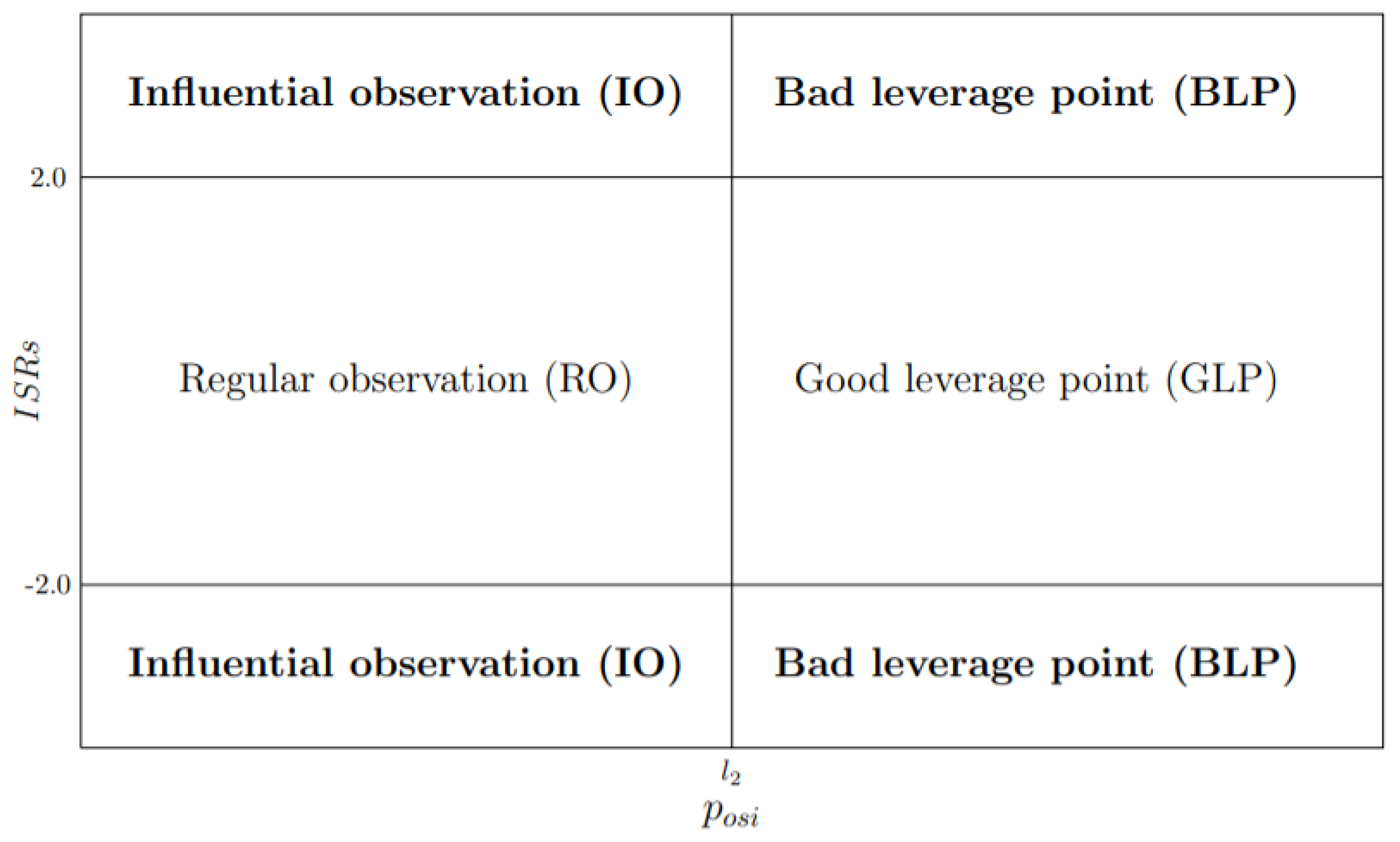
Figure 1 and Figure 2 show the classification of the observations as RO, GLP and IOs according to $ISRs-P_{osi}$ and $ESRs-P_{osi}$, respectively.

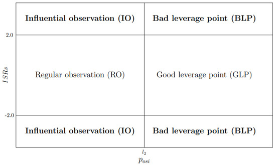
Figure 1. Classification of RO, GLP, and IO according ISRs – P_osi.

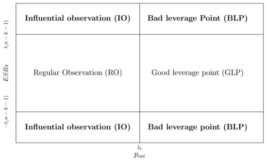
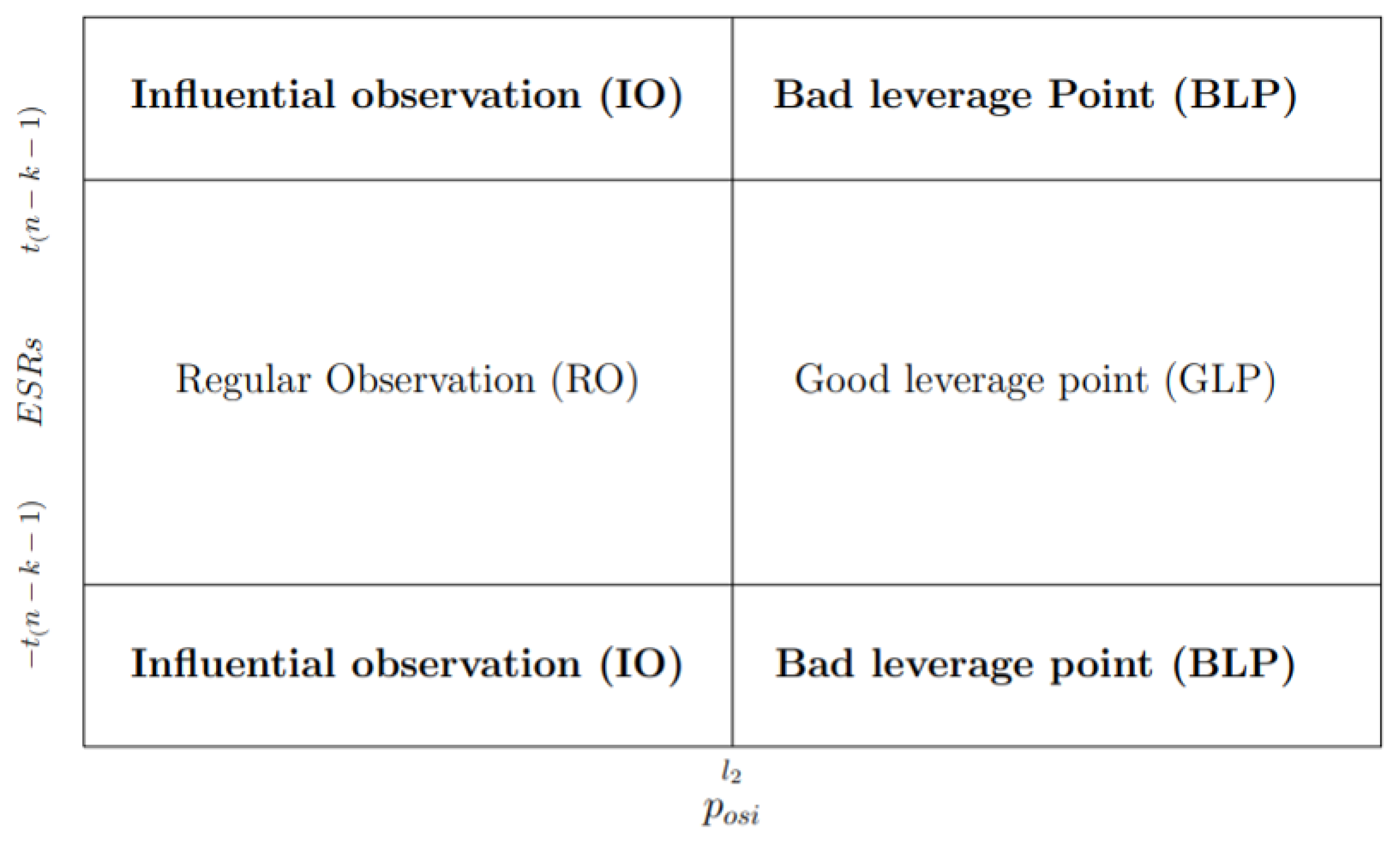
Figure 2. Classification of RO, GLP, and IO according ESRs – P_osi.

(b)

$ESRs-P_{osi}$

i

$i^{th}$ observation is declared RO if $\left|ESRs\right|<t_{n-k-1}$ and $p_{osi}<l_2$.

ii

$i^{th}$ observation is GL if $\left|ESRs\right|<t_{n-k-1}$ and $p_{osi}>l_2$.

iii

$i^{th}$ observation is IO if $\left|ESRs\right|>t_{n-k-1}$ and $p_{si}>l_2$.

iv

$i^{th}$ observation is IO if $\left|ESRs\right|\ge t_{n-k-1}$ and $p_{si}\le l_2$.

4. Results and Discussions

In this section, the performance of all the proposed methods, i.e., the Cook’s Distance (${\widehat{CD}}_{si}$), $H_{si}^2$($H_{si1}^2$(non-robust) and $H_{si2}^2$(robust)), $ISRs-P_{osi}$ and $ESRs-P_{osi}$, is evaluated using a simulation study, artificial data and real datasets of gasoline price data in the southwest area of Sheffield, UK, COVID-19 data in the counties of the State of Georgia, USA and the life expectancy data in counties of the USA.

Simulated Data

We simulated the spatial regression model in Equation (9) for a square spatial grid with sample size, $n=400$, $\rho =0.4$, $\lambda =0.5$ and ${\mathit{W}}_{\mathbf{1}}={\mathit{W}}_{\mathbf{2}}$, using row-standardized Queen’s contiguity spatial weights. ${\mathit{x}}_{\mathbf{0}}=\mathbf{1}$, ${\mathit{x}}_{\mathbf{1}}\sim N\left(0,1\right)$, ${\mathbf{\beta }}_0=0$, ${\mathbf{\beta }}_{\mathbf{1}}=\mathbf{1}$ (bold face 0 and 1 refer to column vectors of values zeros and ones, respectively). The contamination is taken at two percent in each of $\mathit{X}$ and $\mathit{y}$ directions. The contamination in the $\mathit{y}$ direction is taken from the Cauchy distribution because of its fat tails. Contamination in the $\mathit{X}$ direction is taken from the following multivariate distribution,

$$\mathit{X}\sim \left(\left[\begin{array}{c}0\\ 2\end{array}\right], \left[\begin{array}{cc}1& 0\\ 0& 1\end{array}\right]\right)$$

However, it is important to note that during the contamination, some of the contaminations may have attributes similar to those in their neighbourhood, as noted by Dowd [46], and spatial simulation is conditioned to a real dataset.

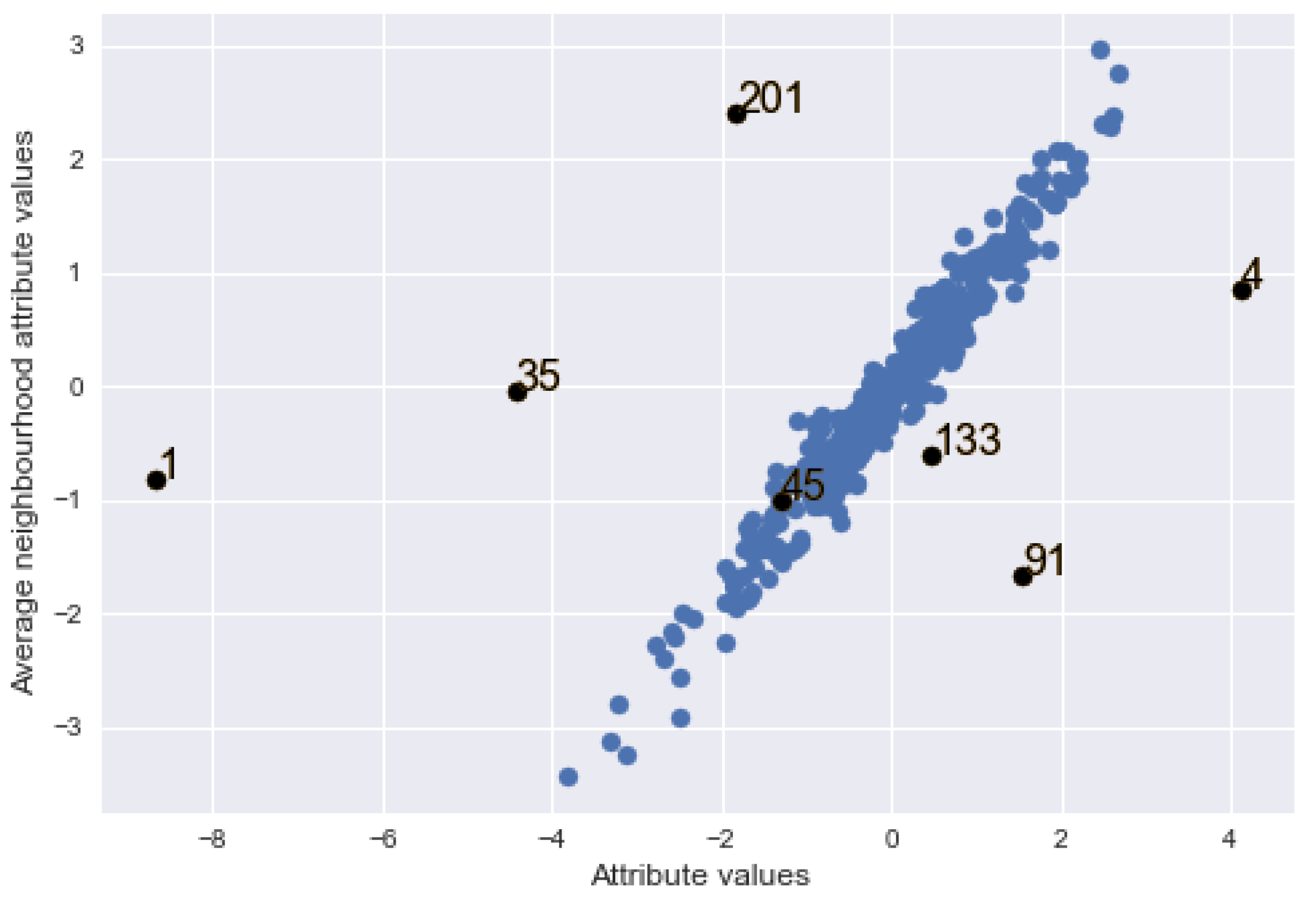
Figure 3 shows the graph of average attribute values in the neighbourhood of locations against their attribute values with added contamination. It can be observed that some of the added contamination, in black dots, are in the middle of clean data points while some stand out from the bulk of the data (i.e., away from their average neighbourhood values), which clearly indicates outlyingness.

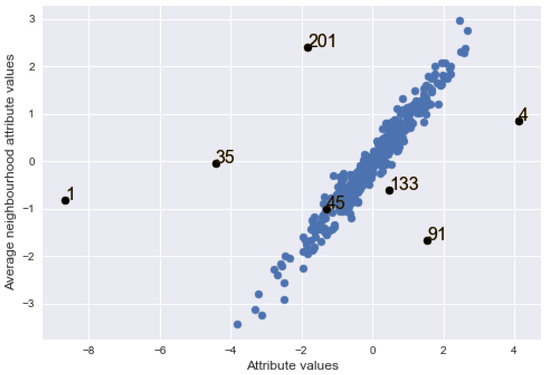
Figure 3. Graph of average attribute values in neighbourhood of locations against the attribute values in the locations with contamination (black points).

Table 1 presents the values of ISRs, ESRs and ${\mathit{p}}_{\mathit{o}\mathit{s}\mathit{i}}$, where values in parentheses are their corresponding cut-off points. It shows seven locations with large Studentized residuals according to ISRs and ESRs. There are 54 observations with large potentials (>0.0078). Two out of the fifty-four potentials correspond to Studentized residuals greater than the thresholds of ISRs and ESRs (locations 51 and 201).

Table 1. ISRs, ESRs and p_osi of locations with large Studentized residuals in the simulated GSM model, with their cut-off points in parentheses.

Location	ISRs (2.00)	ESRs (1.97)	posi (0.0078)
1	15.0378	22.8179	0.0008
4	4.5847	4.7046	0.0033
35	−7.1434	−7.6397	0.0026
51	−4.4695	−4.5801	0.0430
91	4.7613	4.8965	0.0068
201	−6.9336	−7.3840	0.0280
265	−2.2644	−2.2762	0.0068

In order to confirm the outlyingness of the locations classified as spatial IOs, the threshold of each outlier neighbourhood given by

$${\mathrm{med}}_i+3MA{D}_i$$

is computed for the Studentized residuals of the classified location and its immediate neighbourhood, where ${\mathrm{med}}_i$ is the median of the Studentized residuals and $MA{D}_i$ is the median absolute deviation. The absolute value of the Studentized residuals is compared to the neighbourhood threshold for confirmation as an outlier.

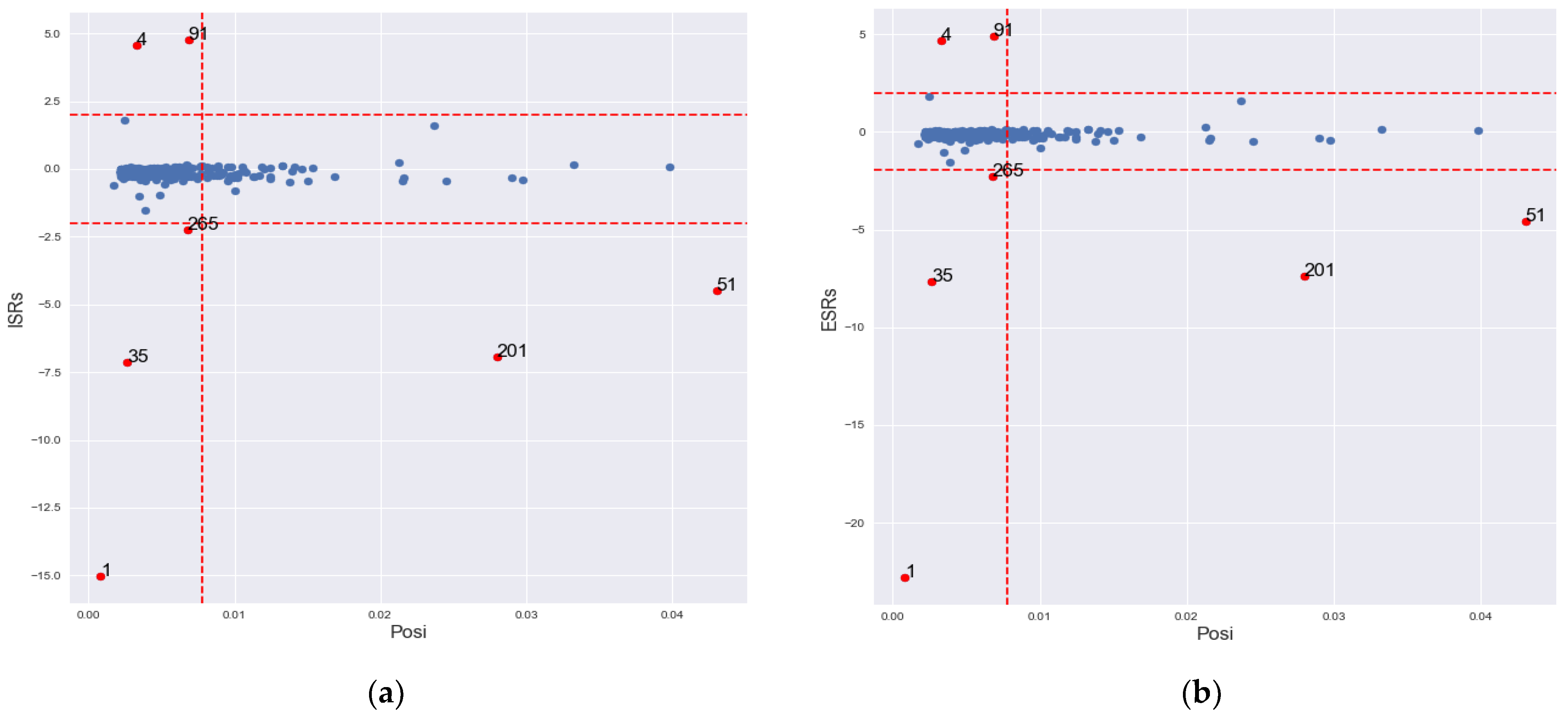
The $C{D}_{si}$ detected location 201, which has large ISRs, ESRs and $p_{si}$. $ISRs-P_{osi}$ and $ESRs-P_{osi}$ classified locations 1, 4, 35, 51, 91, 201 and 265 as IOs. As noted on Figure 4, $ISRs-P_{osi}$ and $ESRs-P_{osi}$ classified locations 1, 4, 35, 91 and 265 as outliers in the $y$ direction, and locations 51 and 201 in both $X$ and $y$ directions. The cut-off limits of $ESRs-P_{osi}$ are narrower than 2 for the 5% cut-off point of the Student’s t-distribution, which is around 1.96 for large sample sizes.

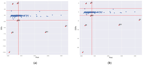
Figure 4. Graph of IO classification according to GLP, BLP and vertical outlier in ISRs – P_osi and ESRs – P_osi for simulated data. (a) ISRs – P_osi; (b) ESRs – P_osi.

$H_{si1}^2$ classified location 1 only as IO. Location 1 has large ISRs and ESRs with small $p_{osi}$. It is an outlier in the $y$ direction. $H_{si2}^2$ identified 60 locations as IOs, including all the locations classified by the other methods. However, a diagnostic examination of the 53 other locations classified by $H_{si2}^2$ alone reveals that all locations that have small ISRs and ESRs with large potential values are classified as IOs. Moreover, the locations with small Studentized residuals, which show no difference with their neighbourhood, are classified as IOs. This is a clear case of swamping, perhaps due the local nature of the spatial IOs.

In a 1000-run of the simulation described above at different error variances of 0.01, 0.1, 0.2 and 0.3 as shown in Table 2, the $C{D}_{si}$ consistently maintained low classification of influential observations with consistent swamping rates of 0%. The $ISRs-P_{osi}$ demonstrated a high detection to the tune of 98% while $ESRs-P_{osi}$ had 100% accurate classification of the IOs, both with swamping rates of 0%. $H_{si1}^2$ had less than 40% accurate classification with zero swamping rate, while the $H_{si2}^2$ had up to 99% accurate IO classification, but usually with very high swamping rates.

Table 2. Influential observations classification rate based on large prediction Studentized residuals and large potentials.

${\mathit{\sigma }}^2$	Method	Accurate Classification (%)	Swamping (%)
	$C{D}_{si}$	22.25	0.0
	$ISRs-P_{osi}$	98.54	0.0
0.01	$ESRs-P_{osi}$	100.00	0.0
	$H_{si1}^2$	39.45	0.0
	$H_{si2}^2$	99.71	81.41
	$C{D}_{si}$	20.64	0.0
	$ISRs-P_{osi}$	98.36	0.0
0.1	$ESRs-P_{osi}$	100.00	0.0
	$H_{si1}^2$	38.09	0.0
	$H_{si2}^2$	99.14	76.48
	$C{D}_{si}$	17.86	0.00
	$ISRs-P_{osi}$	97.51	0.00
0.2	$ESRs-P_{osi}$	100.00	0.00
	$H_{si1}^2$	37.23	0.00
	$H_{si2}^2$	97.34	69.25
	$C{D}_{si}$	16.36	0.00
	$ISRs-P_{osi}$	96.57	0.00
0.3	$ESRs-P_{osi}$	100.00	0.00
	$H_{si1}^2$	36.23	0.00
	$H_{si2}^2$	96.00	64.42

5. Illustrative Examples

5.1. Example 1

The gasoline price data for 61 retail sites in the southwest area of Sheffield from [19] were used in Example 1. The analysis indicated the presence of spatial interaction in the error term with a Moran’s I of 0.239.

The fitted SEM model is given by Equation (21):

$${\widehat{\mathit{y}}}_M=35.78+0.71{\mathit{X}}_F+\widehat{\mathsf{\lambda }}W\mathbf{\xi }$$

(21)

where, ${\mathit{y}}_M$ and ${\mathit{X}}_M$ are the March and February sales from the southwest Sheffield gasoline sale data, respectively, $\widehat{\mathsf{\lambda }}=0.15$ is the estimate of coefficient of correlation in the residuals, $\mathit{W}$ is the standardized weight matrix and $\mathbf{\xi }$ is the vector of correlated residuals.

Table 3 shows the results of the detected IOs in the SEM model for the gasoline data with all the sites detected by the methods. A “yes” under a method column indicates that the site has been detected by the method as IO and a “no” means otherwise. The values in bold in columns ISRs, ESRs and $p_{si}$ indicate large Studentized residuals and potentials greater than 0.0335, respectively. Figure 5 shows the classification of observations by $ISRs-P_{osi}$ and $ESRs-P_{osi}$.

Table 3. Sites with IOs in the analysis of the southwest Sheffield gasoline data.

S/N	Site	ISRs (2.00)	ESRs (2.00)	posi 0.0335	CDsi	ISRs − Posi	ESRs − Posi	$H_{si1}^2$	$H_{si2}^2$
1.	3	−1.8879	−1.9301	0.3538	no	No	No	no	Yes
2.	9	1.4810	1.4962	0.0223	no	No	No	no	Yes
3.	22	1.0127	1.0129	0.0779	no	No	No	no	Yes
4.	25	5.4292	7.5481	0.2773	yes	Yes	Yes	yes	Yes
5.	26	1.4438	1.4573	0.1352	no	No	No	no	Yes
6.	30	2.2054	2.2813	0.2489	no	No	No	no	Yes
7.	40	1.5692	1.5890	0.0194	no	No	No	no	Yes
8.	41	1.1974	1.2058	0.0218	no	No	No	no	Yes
9.	42	−1.9150	−1.9598	0.0378	no	No	No	no	Yes
10.	46	0.1003	0.0995	0.1319	no	No	No	no	Yes
11.	55	−1.2042	−1.2089	0.0219	no	No	No	no	Yes
12.	61	−1.8011	−1.8363	0.0319	no	No	No	no	Yes

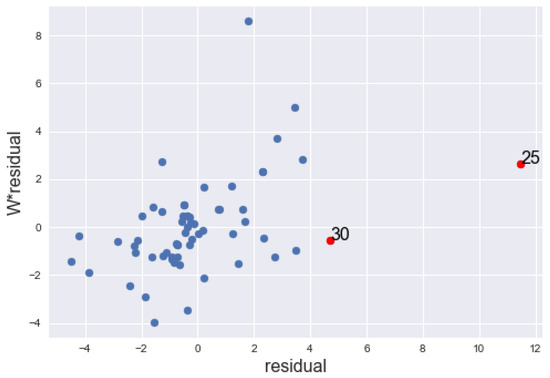
Figure 5. Graph of the lagged residuals against the residuals, of the 61 sites of the southwest Sheffield fitted with SEM, showing the IO points in red dots.

The $C{D}_{si}$, $ISRs-P_{osi}$, $ESRs-P_{osi}$, and $H_{si1}^2$ coincidentally identified site 25 only as IO. $H_{si2}^2$ detects 11 more sites as IOs in addition to site 25. Haining [19] has made elaborate diagnostic analysis of the data where he emphasized the effect of site 25 as IO in the data. Our methods have classified site 30 in addition to location 25 as IO. Figure 5 shows the graph of the lagged residuals against the residuals. It is noticeable from the graph that site 30 has also been marked as an IO.

Though the $H_{si2}^2$ has detected all the suspected IOs, it is prone to swamping. The remaining high potentials are classified as GLP by $ISRs-P_{osi}$ and $ESRs-P_{osi}$ since their Studentized values are small.

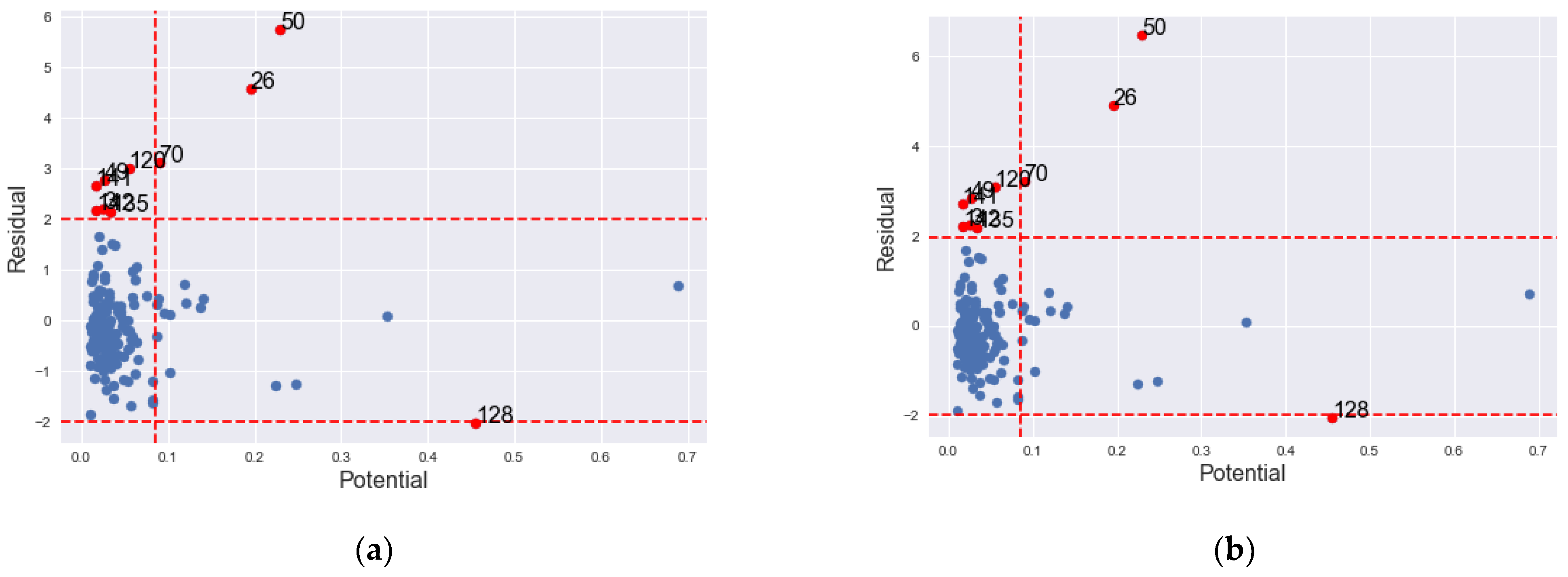
Figure 6 shows the graph of classification of the $ISRs-P_{osi}$ (a) and $ESRs-P_{osi}$ (b) indicating the outliers in red dots, where both are classified as outliers in both the $\mathit{X}$ and $\mathit{y}$ directions.

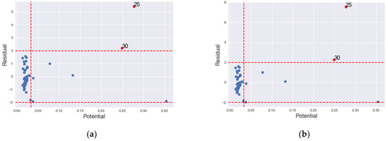
Figure 6. Graph of IO classification according to GLP, BLP and vertical outlier in South West gasoline data. (a) $ISRs-P_{osi}$; (b) $ESRs-P_{osi}$.

5.2. Example 2

The data for example 2 were the COVID-19 data for the 159 counties of the State of Georgia, USA, as of 30 June 2020 (http://dph.georgia.gov/covid-19-daily-status-report; accessed on 30 June 2020) and the health ranking (http://www.countyheathrankings.org; accessed on 30 June 2020). The case-rate per 100,000 of COVID-19 was the dependent variable. The independent variables were the population of black race in the county (${\mathit{X}}_1$), population of Asians (${\mathit{X}}_2$), population of Hispanic (${\mathit{X}}_3$), population of people that are 65 years and above (${\mathit{X}}_4$), population of female in the county (${\mathit{X}}_5$) and life expectancy (${\mathit{X}}_6$).

The model was fitted with the SAR model (model with the lowest Akaike information criteria (AIC) value of 2192). The SAR model is presented in Equation (22):

$$\widehat{\mathit{y}}=\widehat{\mathsf{\rho }}W\widehat{\mathit{y}}+{\widehat{\mathsf{\beta }}}_0+{\displaystyle \sum }_{i=1}^6{\widehat{\mathsf{\beta }}}_i{\mathit{X}}_i$$

(22)

where $\widehat{\mathsf{\rho }}=0.6967$, ${\widehat{\mathsf{\beta }}}_0=1087.7388$, ${\widehat{\mathsf{\beta }}}_1=9.7831$,${\widehat{\mathsf{\beta }}}_2=-6.2210$, ${\widehat{\mathsf{\beta }}}_3=-54.1405$, ${\widehat{\mathsf{\beta }}}_4=-28.5874$, ${\widehat{\mathsf{\beta }}}_5=4.8288$ and ${\widehat{\mathsf{\beta }}}_6=40.3323$. ${\mathit{X}}_1$, ${\mathit{X}}_3$ and $\widehat{\mathsf{\rho }}$ are significant at 5%, while $X_2$ and $X_5$ are significant at 10%. $X_4$ and $X_6$ are not significant.

The Cook’s distance only classified county 50 as an IO. The $ISRs-P_{osi}$ and $ESRs-P_{osi}$ coincided in detecting counties 3, 26, 49, 50, 70, 120, 135, 141 and 142 as IOs. The $H_{si1}^2$ (non-robust) detected 26 and 50 as IOs. The $H_{si2}^2$ (robust) detected 3, 26, 50, 58, 67, 70, 98, 118, 120, 128, 131, 134, 135, 139, 141, 142, 153 and 155 counties. Table 4 shows the detected locations by the various methods with large ISRs, ESRs and high potentials in bold font.

Table 4. Detected IOs counties by different methods in the Georgia COVID-19 data.

County	ISRs (2.00)	ESRs (1.98)	psi 0.0851	CDsi	ISRs – Posi	ESRs – Posi	$H_{si1}^2$	$H_{si2}^2$
3	2.2245	2.2539	0.0257	no	no	no	no	Yes
26	4.5733	4.9060	0.1956	no	yes	yes	yes	Yes
49	2.7685	2.8313	0.0265	no	yes	Yes	no	Yes
50	5.7504	6.4737	0.2298	yes	yes	Yes	yes	Yes
58	0.7090	0.7079	0.6893	no	no	No	yes	Yes
67	0.1018	0.1015	0.3524	no	no	No	no	Yes
70	3.1334	3.2285	0.0895	no	yes	Yes	no	Yes
98	−1.8549	−1.8699	0.0105	no	no	No	no	Yes
118	−1.5657	−1.5731	0.0827	no	no	No	no	Yes
120	3.0168	3.1006	0.0544	no	yes	Yes	no	Yes
128	−2.0152	−2.0359	0.4557	no	yes	yes	no	Yes
131	−1.6718	−1.6862	0.0565	no	no	No	no	Yes
134	−1.6168	−1.6253	0.0818	no	no	No	no	Yes
135	2.1674	2.1942	0.0338	no	yes	Yes	no	Yes
141	2.6726	2.7283	0.0163	no	Yes	yes	no	Yes
142	2.1805	2.2079	0.0174	Yes	yes	no	no	Yes
153	−1.2693	−1.2718	0.2234	No	No	no	no	Yes
155	−1.2334	−1.2359	0.2472	No	No	no	no	Yes

The IOs identified by $ISRs-P_{osi}$ and $ESRs-P_{osi}$ both have large Studentized residuals and large potentials as can be observed in Table 4. Figure 7 shows the outliers in X, y and both X and y directions. The $C{D}_{si}$ detected the largest Studentized residual with a high potential as IO. The $H_{si1}^2$ identified two observations with large Studentized values and high potential values. The $H_{si2}^2$ detected all suspected IOs, but with many having both small values of Studentized residuals and potential values.

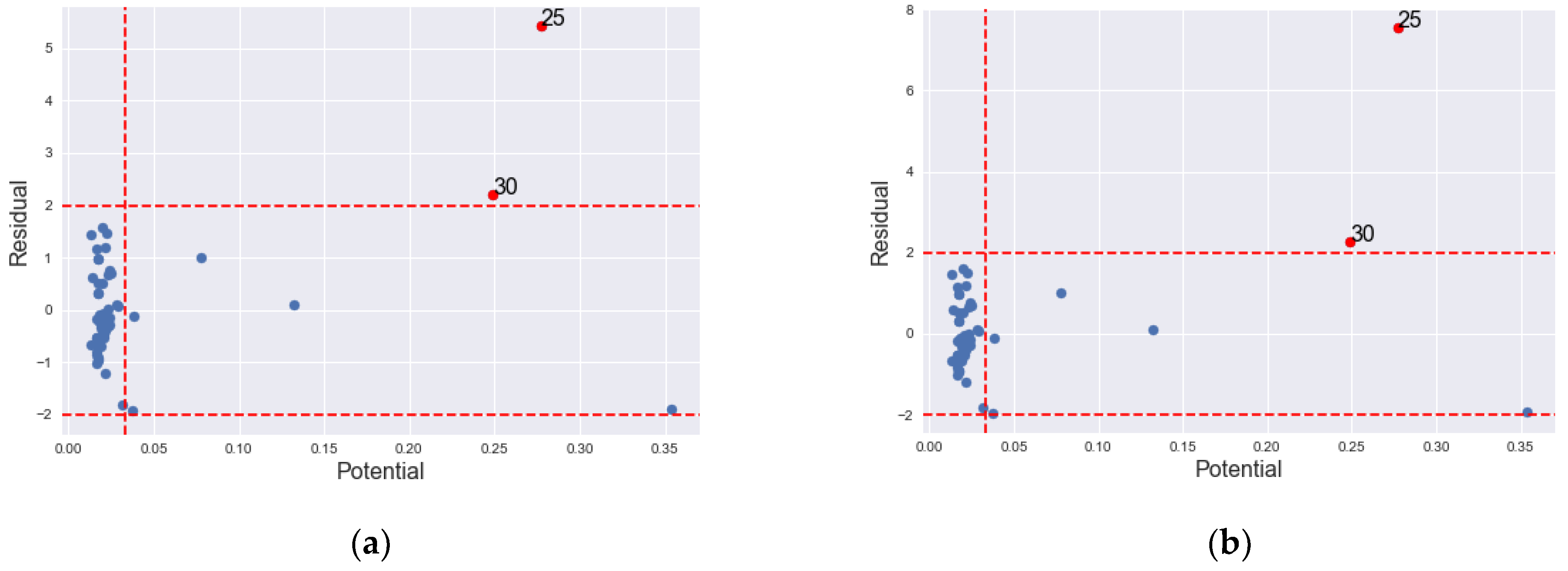
Figure 7. Graph of IO classification according to GLP, BLP and vertical outlier in the State of Georgia, USA COVID-19 data. (a) $ISRs-P_{osi}$; (b) $ESRs-P_{osi}$.

While examining the outlyingness of the classified counties, we find that county 50 is clearly an IO since it has both large Studentized residual and a large potential value. It is outside the threshold value of its neighbourhood.

Four of the counties classified by $ISRs-P_{osi}$ and $ESRs-P_{osi}$(i.e., 26, 50, 70 and 128) are classified as vertical outliers while the counties 3, 49, 120, 135, 141 and 142 have large potential values and Studentized values greater than their threshold values and are classified as BLPs and hence IOs.

Besides the counties classified by $ISRs-P_{osi}$ and $ESRs-P_{osi}$, all the other counties detected by $H_{si2}^2$ have their Studentized difference residuals below their neighbourhood threshold. Though their potential values are mostly large, their prediction Studentized residuals are small in both ISRs and ESRs.

5.3. Example 3

In example 3, the life expectancy of the counties of the US was measured by population density (${\mathit{X}}_1$), fair/poor health status (${\mathit{X}}_2$), obesity (${\mathit{X}}_3$), population in rural area (${\mathit{X}}_4$), inactivity rate (${\mathit{X}}_5$), population of smokers (${\mathit{X}}_6$), population of black people (${\mathit{X}}_7$), population of Asians (${\mathit{X}}_8$) and population of Hawaiians ($X_9$). The data were obtained from the Kaggle website (https://www.kaggle.com/johnjdavisiv/us-counties-covid19-weather-sociohealth-data; accessed on 13 December 2020).

The spatial error model (SEM) had the lowest AIC value and was fitted to the data. The model was significant at the 5% level with a significant Moran’s I of 0.2160. ${\mathit{X}}_1$ and ${\mathit{X}}_4$ were not significant at the 5%. All the other estimates were significant at the 5% level.

The fitted model is given by:

$$\widehat{\mathit{y}}={\widehat{\mathsf{\beta }}}_0+{\displaystyle \sum }_{i=1}^9{\widehat{\mathsf{\beta }}}_i{\mathit{X}}_i+\widehat{\lambda }\mathit{W}\mathbf{\xi }$$

where $\widehat{\mathsf{\lambda }}=0.4343$, ${\widehat{\mathsf{\beta }}}_0=88.4885$, ${\widehat{\mathsf{\beta }}}_1$ = 0.0000, ${\widehat{\mathsf{\beta }}}_2=-0.0954$, ${\widehat{\mathsf{\beta }}}_3=-0.0377$, ${\widehat{\mathsf{\beta }}}_4=0.0040$, ${\widehat{\mathsf{\beta }}}_5=-0.0630$, ${\widehat{\mathsf{\beta }}}_6=-0.3892$, ${\widehat{\mathsf{\beta }}}_7=-0.0113$, ${\widehat{\mathsf{\beta }}}_8=0.1437$, ${\widehat{\mathsf{\beta }}}_9=-0.2016$. Counties with fair/poor health facility had a 0.1 lower life expectancy for an increase in the population. Counties with a larger number of obese people had a decrease in life expectancy of 0.03. Similarly, those counties with a large number of people with inactivity had a life expectancy decreased by 0.06, and counties with a larger number of smokers had a life expectancy decreased by 0.04 per increase in the population. Countries with a higher number of black people and Hawaiians had a life expectancy decreased by 0.01 and 0.2, respectively, while those with a higher number of Asians had an increased rate of 0.14 in population.

The $ISRs-P_{osi}$ classified 139 counties as IOs, while $ESRs-P_{osi}$ classified eight more counties, making a total of 147. $H_{si1}^2$ and $H_{si2}^2$ have classified 24 and 324 counties as IOs, respectively. $C{D}_{si}$ classified no county as IO.

6. Conclusions

In this article, we demonstrated the application of influential observations (IOs) detection techniques from the classical regression to the spatial regression model. Measures that contained spatial information in the spatial autoregression in the dependent variables and residuals were obtained. We also evaluated the performance of some methods employed in classical regression to their spatial counterparts. Though the methods work well in classical regression models, they are mostly prone to either masking or swamping in spatial applications. This is attributable to the local nature of spatial outliers. Hence, we proposed new $ISRs-P_{osi}$ and $ESRs-P_{osi}$ plots to classify observations into four categories: regular observations, vertical outliers, good leverage points and bad leverage points, whereby IOs are those observations which fall in the vertical and bad leverage point categories. Interestingly, the proposed $ESRs-P_{osi}$ diagnostic plot was very successful in classifying observations into the correct categories followed by the $ISRs-P_{osi}$, as demonstrated by the results obtained from a simulation study and real data examples. Thus, the newly established $ESRs-P_{osi}$ plot can be a suitable alternative to identify IOs in the spatial regression model.

References

- Belsley, D.A.; Kuh, E.; Welsch, R.E. Regression Diagnostics: Identifying Influential Data and Sources of Collinearity; John Wiley & Sons: New York, NY, USA, 1980; Volume 571. [Google Scholar]
- Rashid, A.M.; Midi, H.; Slwabi, W.D.; Arasan, J. An Efficient Estimation and Classification Methods for High Dimensional Data Using Robust Iteratively Reweighted SIMPLS Algorithm Based on Nu -Support Vector Regression. IEEE Access 2021, 9, 45955–45967. [Google Scholar] [CrossRef]
- Cook, R.D. Influential Observations in Linear Regression. J. Am. Stat. Assoc. 1977, 74, 169–174. [Google Scholar] [CrossRef]
- Hoaglin, D.C.; Welsch, R.E. The Hat Matrix in Regression and ANOVA. Am. Stat. 1978, 32, 17. [Google Scholar] [CrossRef]
- Andrews, D.F.; Pregibon, D. Finding the Outliers That Matter. J. R. Stat. Soc. Ser. B (Methodol.) 1978, 40, 85–93. [Google Scholar] [CrossRef]
- Hawkins, D.M. Identification of Outliers; Springer: Berlin/Heidelberg, Germany, 1980; Volume 11. [Google Scholar]
- Huber, P. Robust Statistics; John Wiley and Sons: New York, NY, USA, 1981. [Google Scholar]
- Cook, R.D.; Weisberg, S. Monographs on statistics and applied probability. In Residuals and Influence in Regression; Chapman and Hall: New York, NY, USA, 1982; ISBN 978-0-412-24280-9. [Google Scholar]
- Chatterjee, S.; Hadi, A.S. Sensitivity Analysis in Linear Regression; John Wiley & Sons: New York, NY, USA, 1988; Volume 327. [Google Scholar]
- Hadi, A.S. A New Measure of Overall Potential Influence in Linear Regression. Comput. Stat. Data Anal. 1992, 14, 1–27. [Google Scholar] [CrossRef]
- Habshah, M.; Norazan, M.R.; Rahmatullah Imon, A.H.M. The Performance of Diagnostic-Robust Generalized Potentials for the Identification of Multiple High Leverage Points in Linear Regression. J. Appl. Stat. 2009, 36, 507–520. [Google Scholar] [CrossRef]
- Meloun, M.; Militkỳ, J. Statistical Data Analysis: A Practical Guide; Woodhead Publishing Limited: Sawston, Cambridge, UK, 2011. [Google Scholar]
- Puterman, M.L. Leverage and Influence in Autocorrelated Regression Models. J. R. Stat. Soc. Ser. C (Appl. Stat.) 1988, 37, 76–86. [Google Scholar] [CrossRef]
- Schall, R.; Dunne, T.T. A Unified Approach to Outliers in the General Linear Model. Sankhyā Indian J. Stat. Ser. B 1988, 50, 157–167. [Google Scholar]
- Martin, R.J. Leverage, Influence and Residuals in Regression Models When Observations Are Correlated. Commun. Stat.-Theory Methods 1992, 21, 1183–1212. [Google Scholar] [CrossRef]
- Shi, L.; Chen, G. Influence Measures for General Linear Models with Correlated Errors. Am. Stat. 2009, 63, 40–42. [Google Scholar] [CrossRef]
- Cerioli, A.; Riani, M. Robust Transformations and Outlier Detection with Autocorrelated Data. In From Data and Information Analysis to Knowledge Engineering; Spiliopoulou, M., Kruse, R., Borgelt, C., Nürnberger, A., Gaul, W., Eds.; Studies in Classification, Data Analysis, and Knowledge Organization; Springer: Berlin/Heidelberg, Germany, 2006; pp. 262–269. ISBN 978-3-540-31313-7. [Google Scholar]
- Christensen, R.; Johnson, W.; Pearson, L.M. Prediction Diagnostics for Spatial Linear Models. Biometrika 1992, 79, 583–591. [Google Scholar] [CrossRef]
- Haining, R. Diagnostics for Regression Modeling in Spatial Econometrics*. J. Reg. Sci. 1994, 34, 325–341. [Google Scholar] [CrossRef]
- Haining, R.P.; Haining, R. Spatial Data Analysis: Theory and Practice; Cambridge University Press: Cambridge, UK, 2003. [Google Scholar]
- Dai, X.; Jin, L.; Shi, A.; Shi, L. Outlier Detection and Accommodation in General Spatial Models. Stat. Methods Appl. 2016, 25, 453–475. [Google Scholar] [CrossRef]
- Singh, A.K.; Lalitha, S. A Novel Spatial Outlier Detection Technique. Commun. Stat. -Theory Methods 2018, 47, 247–257. [Google Scholar] [CrossRef]
- Anselin, L. Some Robust Approaches to Testing and Estimation in Spatial Econometrics. Reg. Sci. Urban Econ. 1990, 20, 141–163. [Google Scholar] [CrossRef]
- Cerioli, A.; Riani, M. Robust Methods for the Analysis of Spatially Autocorrelated Data. Stat. Methods Appl. 2002, 11, 335–358. [Google Scholar] [CrossRef]
- Yildirim, V.; Mert Kantar, Y. Robust Estimation Approach for Spatial Error Model. J. Stat. Comput. Simul. 2020, 90, 1618–1638. [Google Scholar] [CrossRef]
- Kou, Y.; Lu, C.-T. Outlier Detection, Spatial. In Encyclopedia of GIS; Springer: Boston, MA, USA, 2008; pp. 1539–1546. [Google Scholar]
- Hadi, A.S.; Imon, A.H.M.R. Identification of Multiple Outliers in Spatial Data. Int. J. Stat. Sci. 2018, 16, 87–96. [Google Scholar]
- Hadi, A.S.; Simonoff, J.S. Procedures for the Identification of Multiple Outliers in Linear Models. J. Am. Stat. Assoc. 1993, 88, 1264–1272. [Google Scholar] [CrossRef]
- Aggarwal, C.C. Spatial Outlier Detection. In Outlier Analysis; Springer: New York, NY, USA, 2013; pp. 313–341. ISBN 978-1-4614-6395-5. [Google Scholar]
- Anselin, L. Local Indicators of Spatial Association—LISA. Geogr. Anal. 1995, 27, 93–115. [Google Scholar] [CrossRef]
- Politis, D.; Romano, J.; Wolf, M. Bootstrap Sampling Distributions. In Subsampling; Springer: New York, NY, USA, 1999; Available online: https://link.springer.com/chapter/10.1007/978-1-4612-1554-7_1 (accessed on 16 September 2021).
- Heagerty, P.J.; Lumley, T. Window Subsampling of Estimating Functions with Application to Regression Models. J. Am. Stat. Assoc. 2000, 95, 197–211. [Google Scholar] [CrossRef]
- Anselin, L. Exploratory Spatial Data Analysis and Geographic Information Systems. New Tools Spat. Anal. 1994, 17, 45–54. [Google Scholar]
- Cressie, N.A.C. Statistics for Spatial Data, Rev. ed.; Wiley series in probability and mathematical statistics; Wiley: New York, NY, USA, 1993; ISBN 978-0-471-00255-0. [Google Scholar]
- Anselin, L. Spatial Econometrics: Methods and Models; Studies in Operational Regional Science; Springer: Dordrecht, The Netherlands, 1988; Volume 4, ISBN 978-90-481-8311-1. [Google Scholar]
- LeSage, J.P. The Theory and Practice of Spatial Econometrics; University of Toledo: Toledo, OH, USA, 1999; Volume 28. [Google Scholar]
- Olver, P.J.; Shakiban, C.; Shakiban, C. Applied Linear Algebra; Springer: Berlin/Heidelberg, Germany, 2006; Volume 1. [Google Scholar]
- Horn, R.A.; Johnson, C.R. Matrix Analysis, 2nd ed.; Cambridge University Press: Cambridge, NY, USA, 2012; ISBN 978-0-521-83940-2. [Google Scholar]
- Liesen, J.; Mehrmann, V. Linear Algebra; Springer Undergraduate Mathematics Series; Springer International Publishing: Cham, Germany, 2015; ISBN 978-3-319-24344-3. [Google Scholar]
- Shekhar, S.; Lu, C.-T.; Zhang, P. A Unified Approach to Detecting Spatial Outliers. GeoInformatica 2003, 7, 139–166. [Google Scholar] [CrossRef]
- Billor, N.; Hadi, A.S.; Velleman, P.F. BACON: Blocked Adaptive Computationally Efficient Outlier Nominators. Comput. Stat. Data Anal. 2000, 34, 279–298. [Google Scholar] [CrossRef]
- Imon, A. Identifying Multiple High Leverage Points in Linear Regression. J. Stat. Stud. 2002, 3, 207–218. [Google Scholar]
- Rahmatullah Imon, A.H.M. Identifying Multiple Influential Observations in Linear Regression. J. Appl. Stat. 2005, 32, 929–946. [Google Scholar] [CrossRef]
- Midi, H.; Mohammed, A. The Identification of Good and Bad High Leverage Points in Multiple Linear Regression Model. Math. Methods Syst. Sci. Eng. 2015, 147–158. [Google Scholar]
- Bagheri, A.; Midi, H. Diagnostic Plot for the Identification of High Leverage Collinearity-Influential Observations. Sort: Stat. Oper. Res. Trans. 2015, 39, 51–70. [Google Scholar]
- Dowd, P. The variogram and kriging: Robust and resistant estimators. In Geostatistics for Natural Resources Characterization; Springer: Berlin/Heidelberg, Germany, 1984; pp. 91–106. [Google Scholar]
Publisher’s Note: MDPI stays neutral with regard to jurisdictional claims in published maps and institutional affiliations. |
© 2021 by the authors. Licensee MDPI, Basel, Switzerland. This article is an open access article distributed under the terms and conditions of the Creative Commons Attribution (CC BY) license (https://creativecommons.org/licenses/by/4.0/).