On a New Construction of Generalized q-Bernstein Polynomials Based on Shape Parameter λ

Abstract

This paper deals with several approximation properties for a new class of q-Bernstein polynomials based on new Bernstein basis functions with shape parameter $\lambda$ on the symmetric interval $[-1,1]$. Firstly, we computed some moments and central moments. Then, we constructed a Korovkin-type convergence theorem, bounding the error in terms of the ordinary modulus of smoothness, providing estimates for Lipschitz-type functions. Finally, with the aid of Maple software, we present the comparison of the convergence of these newly constructed polynomials to the certain functions with some graphical illustrations and error estimation tables.

1. Introduction

Quantum calculus, briefly q-calculus, has many applications in various disciplines such as mechanics, physics, mathematics, and so on. In approximation theory, a generalization of Bernstein polynomials based on q-calculus was firstly introduced by Lupaş [1]. In 1997, Phillips [2] proposed some convergence theorems and Voronovskaya-type asymptotic formulae for the most popular generalizations of the q-Bernstein polynomials. Now, before proceeding further, let us recall the certain notations on q-calculus (for more details, see [3]). Let $0<q\le 1$, for all integers $j>0$; the q-integer ${\left[j\right]}_q$ is given by:

$${\left[j\right]}_q:=\left\{\begin{array}{c}\frac{1-q^j}{1-q},q\ne 1\\ j,q=1\end{array}.\right.$$

The q-factorial ${\left[j\right]}_q!$ and q-binomial ${\left[\genfrac{}{}{0.0pt}{}{j}{l}\right]}_q$ are defined, respectively, as below:

$${\left[j\right]}_q!:=\left\{\begin{array}{c}{\left[j\right]}_q{\left[j-1\right]}_q..{\left[1\right]}_q,j=1,2,..\\ 1,j=0\end{array}\right.$$

and:

$${\left[\genfrac{}{}{0.0pt}{}{j}{l}\right]}_q:=\frac{{\left[j\right]}_q!}{{\left[l\right]}_q!{\left[j-l\right]}_q!},(j\ge l\ge 0).$$

Let $a,b,m\in \mathbb{N},$ $0\le a\le b,$ $y\in [0,\frac{{[m+a]}_q}{{[m+b]}_q}]$, then following the polynomials introduced by Karahan and Izgi [4]:

$$F_{m,a,b}(\mu ;q,y)=\stackrel{m}{{\displaystyle \sum }_{j=0}}\mu \left(\frac{{\left[j\right]}_q{[m+a]}_q}{{\left[m\right]}_q{[m+b]}_q}\right)u_{m,j,a,b}(y;q),$$

(1)

where the generalized q-Bernstein basis functions $u_{m,j,a,b}$ are defined as:

$$u_{m,j,a,b}(y;q)={\left(\frac{{[m+a]}_q}{{[m+b]}_q}\right)}^m{\left[\genfrac{}{}{0.0pt}{}{m}{j}\right]}_q{y}^j\underset{r=0}{{\displaystyle \prod }^{m-j-1}}(\frac{{[m+a]}_q}{{[m+b]}_q}-q^{r}y).$$

(2)

They investigated some approximation properties of polynomials (1) and estimated the order of convergence in terms of the moduli of continuity. For some recent works related to linear positive operators, we refer to [5,6,7,8,9,10,11,12,13,14]. Additionally, one can refer to [15,16,17] for some notable results with special polynomials based on the q- and $(p,q)$-integers.

Basis functions with desirable properties have an important role in Computer-Aided Geometric Design (CAGD) and computer graphics in order to construct surfaces and curves. The Bernstein polynomial basis was studied and used in many papers. An extensive study about this topic was given by Farouki in the survey paper [18]. These basis functions are widely addressed in many applications areas such as the numerical solution of partial differential equations, CAGD, font design, and 3D modeling. For some applications in CAGD, we refer to [19,20,21,22].

Very recently, the Bernstein basis with shape parameter $\lambda \in [-1,1]$, which was introduced by Ye et al. [23], has attracted the interest of and in as short a time was studied by a number of researchers.

In the year 2019, Cai et al. [24] obtained several statistical approximation properties of a new generalization of $(\lambda ,q)$-Bernstein polynomials as follows:

$$B_m(\mu ;\lambda ,y)=\sum _{j=0}^m{\tilde{r}}_{m,j}(\lambda ;y,q)\mu \left(\frac{{\left[j\right]}_q}{{\left[m\right]}_q}\right),$$

(3)

where $m\ge 2,$ $y\in [0,1],$ $0<q\le 1$, and ${\tilde{r}}_{m,j}(\lambda ;y,q)$ are the Bernstein basis with shape parameter $\lambda \in [-1,1].$

In [25], Acu et al. established several approximation properties of the Kantorovich kind $\lambda$-Bernstein polynomials and estimated the order of approximation with the aid of the Ditzian–Totik modulus of smoothness. Srivastava et al. [26] proposed and studied a Stancu variant of $\lambda$-Bernstein polynomials and examined the uniform convergence, global approximation result, and Voronovskaya’s approximation theorems. Moreover, Özger [27] investigated some statistical approximation properties of univariate and bivariate occasions of $\lambda$-Bernstein polynomials. In [28], Mursaleen et al. considered a Chlodowsky variant of $(\lambda ,q)$-Bernstein–Stancu polynomials and proved the uniform convergence and Voronovskaya-type asymptotic theorems for these polynomials. For some recent relevant papers, see [29,30,31,32,33,34,35,36,37,38,39,40].

Inspired by all the above-mentioned works, we now construct the following polynomials with shape parameter $\lambda \in [-1,1]:$

$$F_{m,a,b}(\mu ;\lambda ,q,y)=\stackrel{m}{{\displaystyle \sum }_{j=0}}\mu \left(\frac{{\left[j\right]}_q{[m+a]}_q}{{\left[m\right]}_q{[m+b]}_q}\right){\tilde{u}}_{m,j,a,b}(y;q),$$

(4)

where:

$$\begin{array}{cc}\hfill {\tilde{u}}_{m,0,a,b}(y;q)& =u_{m,0,a,b}(y;q)-\frac{\lambda }{{\left[m\right]}_q+1}{u}_{m+1,1,a,b}(y;q),\hfill \\ \hfill {\tilde{u}}_{m,j,a,b}(y;q)& =u_{m,j,a,b}(y;q)+\lambda \left(\frac{{\left[m\right]}_q-2{\left[j\right]}_q+1}{{\left[m\right]}_q^2-1}{u}_{m+1,j,a,b}(y;q)\right.\hfill \end{array}$$

$$-\left.\frac{{\left[m\right]}_q-2{\left[j\right]}_q-1}{{\left[m\right]}_q^2-1}{u}_{m+1,j+1,a,b}(y;q)\right)(j=1,2,...,m-1),$$

(5)

$${\tilde{u}}_{m,m,a,b}(y;q)=u_{m,m,a,b}(y;q)-\frac{\lambda }{{\left[m\right]}_q+1}{u}_{m+1,m,a,b}(y;q),$$

where $m\ge 2,$ $0\le a\le b,$ $y\in [0,\frac{{[m+a]}_q}{{[m+b]}_q}]$, $0<q\le 1$, and $u_{m,j,a,b}(y;q)$, defined as in (2).

Many researchers have investigated iterated Boolean sums of positive operators since these operators have the possibility of accelerating the convergence with respect to the originating positive operators (see [41,42,43]). There are certain important papers in this context in which the authors established global direct, inverse, and saturation results for the convergence of iterated Boolean sums of Bernstein operators to the identity operator. One may obtain further results about the saturation order of approximating polynomials defined in this paper as a future study.

The present work is organized as follows: In Section 2, we calculate some preliminary results such as moments and central moments. In Section 3, we give a Korovkin-type convergence theorem, bind the error in terms of the ordinary modulus of smoothness, and provide estimates for Lipschitz-type functions. In the final section, with the help of the Maple software, we present the comparison of the convergence polynomials (4) with the different values of the $a,b,m,q$, and $\lambda$ parameters with some graphs and error estimation tables.

2. Preliminaries

This section is devoted to calculating some necessary results such as the moments and central moments of polynomials (4).

Lemma 1

([4]). Let $e_i\left(y\right)=y^i,(i=0,1,2,3,4)$, be the test functions. Then, the polynomials (1) satisfy:

$$\begin{array}{cc}\hfill F_{m,a,b}(e_0;q,y)& =1,\hfill \\ \hfill F_{m,a,b}(e_1;q,y)& =y,\hfill \\ \hfill F_{m,a,b}(e_2;q,y)& =y^2+\frac{y\left({[m+a]}_q-{[m+b]}_{q}y\right)}{{\left[m\right]}_q{[m+b]}_q}.\hfill \end{array}$$

Lemma 2.

Let $y\in [0,\frac{{[m+a]}_q}{{[m+b]}_q}],$ $0<q\le 1,$ $\lambda \in [-1,1]$, and $m>1.$ Then, we obtain:

$$F_{m,a,b}(e_0;\lambda ,q,y)=1.$$

(6)

Proof. 

In view of the relation ${\left[m\right]}_q=q{[m-1]}_q+1,$ we obtain:

$$\begin{array}{cc}\hfill & \sum _{j=0}^m{\tilde{u}}_{m,j,a,b}(y;\lambda ,q)\hfill \\ \hfill & =\sum _{j=0}^m{u}_{m,j,a,b}(y;q)-\frac{\lambda }{{\left[m\right]}_q+1}{u}_{m+1,1,a,b}(y;q)+\lambda \frac{{\left[m\right]}_q-2{\left[1\right]}_q+1}{{\left[m\right]}_q^2-1}{u}_{m+1,1,a,b}(y;q)\hfill \\ \hfill & -\lambda \frac{{\left[m\right]}_q-2q{\left[1\right]}_q-1}{{\left[m\right]}_q^2-1}{u}_{m+1,2,a,b}(y;q)+\lambda \frac{{\left[m\right]}_q-2{\left[2\right]}_q+1}{{\left[m\right]}_q^2-1}{u}_{m+1,2,a,b}(y;q)\hfill \\ \hfill & -\lambda \frac{{\left[m\right]}_q-2q{\left[2\right]}_q-1}{{\left[m\right]}_q^2-1}{u}_{m+1,3,a,b}(y;q)...+\lambda \frac{{\left[m\right]}_q-2{[m-1]}_q+1}{{\left[m\right]}_q^2-1}{u}_{m+1,m-1,a,b}(y;q)\hfill \\ \hfill & -\lambda \frac{{\left[m\right]}_q-2q{[m-1]}_q-1}{{\left[m\right]}_q^2-1}{u}_{m+1,m,a,b}(y;q)-\frac{\lambda }{{\left[m\right]}_q+1}{u}_{m+1,m,a,b}(y;q)\hfill \\ \hfill & =\sum _{j=0}^m{u}_{m,j,a,b}(y;q)+\lambda \frac{2q{[m-1]}_q-{\left[m\right]}_q+1}{{\left[m\right]}_q^2-1}{u}_{m+1,m,a,b}(y;q)\hfill \\ \hfill & -\frac{\lambda }{{\left[m\right]}_q+1}{u}_{m+1,m,a,b}(y;q)\hfill \\ \hfill & =\sum _{j=0}^m{u}_{m,j,a,b}(y;q)=1.\hfill \end{array}$$

Hence, we have identity (6). □

Lemma 3.

Let $y\in [0,\frac{{[m+a]}_q}{{[m+b]}_q}],$ $0<q\le 1,$ $\lambda \in [-1,1]$, and $m>1.$ Then, one has:

$$\begin{array}{cc}\hfill & F_{m,a,b}(e_1;\lambda ,q,y)=y+\frac{{[m+1]}_q\lambda \left(1-{\left(\frac{{[m+b]}_q}{{[m+a]}_q}y\right)}^m\right)}{{\left[m\right]}_q({\left[m\right]}_q-1)}\hfill \\ \hfill & +\frac{2{[m+b]}_q}{{[m+a]}_q}\frac{{[m+1]}_q\lambda y}{{\left[m\right]}_q^2-1}\left(\frac{1-y^m}{{\left[m\right]}_q}+qy\frac{{[m+b]}_q}{{[m+a]}_q}(1-y^{m-1})\right)\hfill \\ \hfill & +\frac{{[m+a]}_q}{{[m+b]}_q}\frac{\lambda }{q{\left[m\right]}_q({\left[m\right]}_q+1)}\left(1-{\left(\frac{{[m+b]}_q}{{[m+a]}_q}\right)}^{m+1}\stackrel{m}{{\displaystyle \prod }_{r=0}}\left(\frac{{[m+a]}_q}{{[m+b]}_q}-q^{r}y\right)\right.\hfill \\ \hfill & \left.-{\left(\frac{{[m+b]}_q}{{[m+a]}_q}y\right)}^{m+1}-{[m+1]}_{q}y\frac{{[m+b]}_q}{{[m+a]}_q}\left(1-{\left(\frac{{[m+b]}_q}{{[m+a]}_q}y\right)}^m\right)\right)\hfill \\ \hfill & +\frac{\lambda }{{\left[m\right]}_q^2-1}\left\{\frac{2{[m+1]}_q{[m+b]}_q{y}^2}{{[m+a]}_q}\left(1-{\left(\frac{{[m+b]}_q}{{[m+a]}_q}y\right)}^{m-1}\right)\right.\hfill \\ \hfill & -\frac{2{[m+1]}_{q}y}{q{\left[m\right]}_q}\left(1-{\left(\frac{{[m+b]}_q}{{[m+a]}_q}y\right)}^m\right)+\frac{2{[m+a]}_q}{q{\left[m\right]}_q{[m+b]}_q}\left(1-{\left(\frac{{[m+b]}_q}{{[m+a]}_q}y\right)}^{m+1}\right)\hfill \\ \hfill & \left.-{\left(\frac{{[m+b]}_q}{{[m+a]}_q}\right)}^{m+1}\stackrel{m}{{\displaystyle \prod }_{r=0}}\left(\frac{{[m+a]}_q}{{[m+b]}_q}-q^{r}y\right)\right\}.\hfill \end{array}$$

(7)

Proof. 

$$\begin{array}{cc}\hfill F_{m,a,b}(e_1;\lambda ,q,y)& =\sum _{j=0}^m\frac{{\left[j\right]}_q{[m+a]}_q}{{\left[m\right]}_q{[m+b]}_q}{\tilde{u}}_{m,j,a,b}(y;\lambda ,q)\hfill \\ \hfill & =\sum _{j=0}^{m-1}\frac{{\left[j\right]}_q{[m+a]}_q}{{\left[m\right]}_q{[m+b]}_q}{\tilde{u}}_{m,j,a,b}(y;\lambda ,q)+{\tilde{u}}_{m,m,a,b}(y;\lambda ,q)\hfill \\ \hfill & =\sum _{j=0}^{m-1}\frac{{\left[j\right]}_q{[m+a]}_q}{{\left[m\right]}_q{[m+b]}_q}\left\{\lambda \frac{{\left[m\right]}_q-2{\left[j\right]}_q+1}{{\left[m\right]}_q^2-1}{u}_{m+1,j,a,b}(y;q)\right.\hfill \\ \hfill & \left.-\lambda \frac{{\left[m\right]}_q-2q{\left[j\right]}_q-1}{{\left[m\right]}_q^2-1}{u}_{m+1,j+1,a,b}(y;q)\right\}\hfill \\ \hfill & +u_{m,m,a,b}(y;q)-\frac{\lambda }{{\left[m\right]}_q+1}{u}_{m+1,m,a,b}(y;q)\hfill \\ \hfill & =\sum _{j=0}^m\frac{{\left[j\right]}_q{[m+a]}_q}{{\left[m\right]}_q{[m+b]}_q}{u}_{m,j,a,b}(y;q)\hfill \\ \hfill & +\lambda \sum _{j=0}^m\frac{{\left[j\right]}_q{[m+a]}_q}{{\left[m\right]}_q{[m+b]}_q}\frac{{\left[m\right]}_q-2{\left[j\right]}_q+1}{{\left[m\right]}_q^2-1}{u}_{m+1,j,a,b}(y;q)\hfill \\ \hfill & -\lambda \sum _{j=1}^{m-1}\frac{{\left[j\right]}_q{[m+a]}_q}{{\left[m\right]}_q{[m+b]}_q}\frac{{\left[m\right]}_q-2q{\left[j\right]}_q-1}{{\left[m\right]}_q^2-1}{u}_{m+1,j+1,a,b}(y;q).\hfill \end{array}$$

It is known from Karahan and Izgi [4] that ${\displaystyle \sum _{j=0}^m}\frac{{\left[j\right]}_q{[m+a]}_q}{{\left[m\right]}_q{[m+b]}_q}{u}_{m,j,a,b}(y;q)=y$; thus:

$$\begin{array}{cc}\hfill & F_{m,a,b}(e_1;\lambda ,q,y)\hfill \\ \hfill & =y+\lambda \frac{{[m+1]}_q}{{\left[m\right]}_q({\left[m\right]}_q-1)}\sum _{j=1}^m\frac{{\left[j\right]}_q{[m+a]}_q}{{[m+1]}_q{[m+b]}_q}\frac{{[m+1]}_q!}{{\left[j\right]}_q!{[m+1-j]}_q!}{\left(\frac{{[m+b]}_q}{{[m+a]}_q}\right)}^{m+1}{y}^j\hfill \\ \hfill & .\stackrel{m-j}{{\displaystyle \prod }_{r=0}}\left(\frac{{[m+a]}_q}{{[m+b]}_q}-q^{r}y\right)\hfill \\ \hfill & -2\lambda \frac{{[m+1]}_q}{{\left[m\right]}_q^2-1}\sum _{j=1}^m\frac{{\left[j\right]}_q^2{[m+a]}_q}{{\left[m\right]}_q{[m+1]}_q{[m+b]}_q}\frac{{[m+1]}_q!}{{\left[j\right]}_q!{[m+1-j]}_q!}{\left(\frac{{[m+b]}_q}{{[m+a]}_q}\right)}^{m+1}{y}^j\hfill \\ \hfill & .\stackrel{m-j}{{\displaystyle \prod }_{r=0}}\left(\frac{{[m+a]}_q}{{[m+b]}_q}-q^{r}y\right)\hfill \\ \hfill & -\lambda \frac{{[m+1]}_q}{{\left[m\right]}_q({\left[m\right]}_q+1)}\sum _{j=1}^{m-1}\frac{{\left[j\right]}_q{[m+a]}_q}{{[m+1]}_q{[m+b]}_q}\frac{{[m+1]}_q!}{{[j+1]}_q!{[m-j]}_q!}{\left(\frac{{[m+b]}_q}{{[m+a]}_q}\right)}^{m+1}{y}^{j+1}\hfill \\ \hfill & .\stackrel{m-j-1}{{\displaystyle \prod }_{r=0}}\left(\frac{{[m+a]}_q}{{[m+b]}_q}-q^{r}y\right)\hfill \\ \hfill & +2q\lambda \frac{{[m+1]}_q}{{\left[m\right]}_q^2-1}\sum _{j=1}^{m-1}\frac{{\left[j\right]}_q^2{[m+a]}_q}{{\left[m\right]}_q{[m+1]}_q{[m+b]}_q}\frac{{[m+1]}_q!}{{[j+1]}_q!{[m-j]}_q!}{\left(\frac{{[m+b]}_q}{{[m+a]}_q}\right)}^{m+1}{y}^{j+1}\hfill \\ \hfill & .\stackrel{m-j-1}{{\displaystyle \prod }_{r=0}}\left(\frac{{[m+a]}_q}{{[m+b]}_q}-q^{r}y\right)=:y+{\Omega }_1+{\Omega }_2+{\Omega }_3+{\Omega }_4.\hfill \end{array}$$

(8)

Now, we calculate the identities ${\Omega }_1,$ ${\Omega }_2,$ ${\Omega }_3$, and ${\Omega }_4$, respectively.

$$\begin{array}{cc}\hfill {\Omega }_1& =\lambda \frac{{[m+1]}_q}{{\left[m\right]}_q({\left[m\right]}_q-1)}\sum _{j=1}^m\frac{{\left[j\right]}_q{[m+a]}_q}{{[m+1]}_q{[m+b]}_q}\frac{{[m+1]}_q!}{{\left[j\right]}_q!{[m+1-j]}_q!}{\left(\frac{{[m+b]}_q}{{[m+a]}_q}\right)}^{m+1}{y}^j\hfill \\ \hfill & .\stackrel{m-j}{{\displaystyle \prod }_{r=0}}\left(\frac{{[m+a]}_q}{{[m+b]}_q}-q^{r}y\right)\hfill \\ \hfill & =\lambda \frac{{[m+1]}_q}{{\left[m\right]}_q({\left[m\right]}_q-1)}\sum _{j=1}^m{u}_{m,j,a,b}(y;q)=\lambda \frac{{[m+1]}_q\left(1-{\left(\frac{{[m+b]}_q}{{[m+a]}_q}y\right)}^m\right)}{{\left[m\right]}_q({\left[m\right]}_q-1)}.\hfill \end{array}$$

(9)

Next, using the expression ${\left[j\right]}_q^2=q{\left[j\right]}_q{[j-1]}_q+{\left[j\right]}_q,$ it follows:

$$\begin{array}{cc}\hfill {\Omega }_2& =-2\lambda \frac{{[m+1]}_q}{{\left[m\right]}_q^2-1}\sum _{j=1}^m\frac{{\left[j\right]}_q^2{[m+a]}_q}{{\left[m\right]}_q{[m+1]}_q{[m+b]}_q}\frac{{[m+1]}_q!}{{\left[j\right]}_q!{[m+1-j]}_q!}{\left(\frac{{[m+b]}_q}{{[m+a]}_q}\right)}^{m+1}{y}^j\hfill \\ \hfill & .\stackrel{m-j}{{\displaystyle \prod }_{r=0}}\left(\frac{{[m+a]}_q}{{[m+b]}_q}-q^{r}y\right)\hfill \\ \hfill & =-2q\lambda \frac{{[m+1]}_q}{{\left[m\right]}_q^2-1}\sum _{j=1}^m\frac{{\left[j\right]}_q{[j-1]}_q}{{\left[m\right]}_q{[m+1]}_q}\frac{{[m+1]}_q!}{{\left[j\right]}_q!{[m+1-j]}_q!}{\left(\frac{{[m+b]}_q}{{[m+a]}_q}\right)}^m{y}^j\hfill \\ \hfill & .\stackrel{m-j}{{\displaystyle \prod }_{r=0}}\left(\frac{{[m+a]}_q}{{[m+b]}_q}-q^{r}y\right)-2\lambda \frac{{[m+1]}_q}{{\left[m\right]}_q^2-1}\sum _{j=1}^m\frac{{\left[j\right]}_q}{{\left[m\right]}_q{[m+1]}_q}\frac{{[m+1]}_q!}{{\left[j\right]}_q!{[m+1-j]}_q!}\hfill \\ \hfill & .{\left(\frac{{[m+b]}_q}{{[m+a]}_q}\right)}^m{y}^j\stackrel{m-j}{{\displaystyle \prod }_{r=0}}\left(\frac{{[m+a]}_q}{{[m+b]}_q}-q^{r}y\right)\hfill \\ \hfill & =-\frac{{[m+b]}_q}{{[m+a]}_q}\frac{2q\lambda {[m+1]}_q}{{\left[m\right]}_q^2-1}{y}^2\sum _{j=0}^{m-2}{u}_{m-1,j,a,b}(y;q)-\frac{2\lambda {[m+1]}_q}{{\left[m\right]}_q\left({\left[m\right]}_q^2-1\right)}y\sum _{j=0}^{m-1}{u}_{m,j,a,b}(y;q)\hfill \\ \hfill & =\frac{2{[m+b]}_q}{{[m+a]}_q}\frac{{[m+1]}_q\lambda y}{{\left[m\right]}_q^2-1}\left(\frac{1-y^m}{{\left[m\right]}_q}+qy\frac{{[m+b]}_q}{{[m+a]}_q}(1-y^{m-1})\right).\hfill \end{array}$$

(10)

Furthermore, if we use expression ${\left[j\right]}_q={[j+1]}_q/q-1/q,$ then:

$$\begin{array}{cc}\hfill {\Omega }_3& =-\lambda \frac{{[m+1]}_q}{{\left[m\right]}_q({\left[m\right]}_q+1)}\sum _{j=1}^{m-1}\frac{{\left[j\right]}_q}{{[m+1]}_q}\frac{{[m+1]}_q!}{{[j+1]}_q!{[m-j]}_q!}\hfill \\ \hfill & ·{\left(\frac{{[m+b]}_q}{{[m+a]}_q}\right)}^m{y}^{j+1}\stackrel{m-j-1}{{\displaystyle \prod }_{r=0}}\left(\frac{{[m+a]}_q}{{[m+b]}_q}-q^{r}y\right)\hfill \\ \hfill & =\frac{{[m+a]}_q}{{[m+b]}_q}\frac{\lambda }{q{\left[m\right]}_q({\left[m\right]}_q+1)}\sum _{j=1}^{m-1}{u}_{m+1,j+1,a,b}(y;q)-\frac{\lambda {[m+1]}_q}{q{\left[m\right]}_q({\left[m\right]}_q+1)}\sum _{j=1}^{m-1}{u}_{m,j,a,b}(y;q)\hfill \\ \hfill & =\frac{{[m+a]}_q}{{[m+b]}_q}\frac{\lambda }{q{\left[m\right]}_q({\left[m\right]}_q+1)}\left(1-{\left(\frac{{[m+b]}_q}{{[m+a]}_q}\right)}^m{[m+1]}_{q}y\stackrel{m-1}{{\displaystyle \prod }_{r=0}}\left(\frac{{[m+a]}_q}{{[m+b]}_q}-q^{r}y\right)\right.\hfill \\ \hfill & \left.-{\left(\frac{{[m+b]}_q}{{[m+a]}_q}\right)}^{m+1}\stackrel{m}{{\displaystyle \prod }_{r=0}}\left(\frac{{[m+a]}_q}{{[m+b]}_q}-q^{r}y\right)-{\left(\frac{{[m+b]}_q}{{[m+a]}_q}y\right)}^{m+1}\right)\hfill \end{array}$$

$$\begin{array}{c}\hfill \\ \hfill & -\frac{\lambda {[m+1]}_{q}y}{q{\left[m\right]}_q({\left[m\right]}_q+1)}\left(1-{\left(\frac{{[m+b]}_q}{{[m+a]}_q}\right)}^m\stackrel{m-1}{{\displaystyle \prod }_{r=0}}\left(\frac{{[m+a]}_q}{{[m+b]}_q}-q^{r}y\right)-{\left(\frac{{[m+b]}_q}{{[m+a]}_q}y\right)}^m\right)\hfill \\ \hfill & =\frac{{[m+a]}_q}{{[m+b]}_q}\frac{\lambda }{q{\left[m\right]}_q({\left[m\right]}_q+1)}\left(1-{\left(\frac{{[m+b]}_q}{{[m+a]}_q}\right)}^{m+1}\stackrel{m}{{\displaystyle \prod }_{r=0}}\left(\frac{{[m+a]}_q}{{[m+b]}_q}-q^{r}y\right)\right.\hfill \\ \hfill & \left.-{\left(\frac{{[m+b]}_q}{{[m+a]}_q}y\right)}^{m+1}-{[m+1]}_{q}y\frac{{[m+b]}_q}{{[m+a]}_q}\left(1-{\left(\frac{{[m+b]}_q}{{[m+a]}_q}y\right)}^m\right)\right).\hfill \end{array}$$

(11)

Lastly, taking ${\left[j\right]}_q^2={\left[j\right]}_q{[j+1]}_q/q-{\left[j\right]}_q/q$ into account, it follows:

$$\begin{array}{cc}\hfill {\Omega }_4& =\frac{2q\lambda {[m+1]}_q}{{\left[m\right]}_q^2-1}\sum _{j=1}^{m-1}\frac{{\left[j\right]}_q^2}{{\left[m\right]}_q{[m+1]}_q}\frac{{[m+1]}_q!}{{[j+1]}_q!{[m-j]}_q!}\hfill \\ \hfill & ·{\left(\frac{{[m+b]}_q}{{[m+a]}_q}\right)}^m{y}^{j+1}\stackrel{m-j-1}{{\displaystyle \prod }_{r=0}}\left(\frac{{[m+a]}_q}{{[m+b]}_q}-q^{r}y\right)\hfill \\ \hfill & =\frac{2\lambda {[m+1]}_q}{{\left[m\right]}_q^2-1}\frac{{[m+b]}_q}{{[m+a]}_q}{y}^2\sum _{j=0}^{m-2}{u}_{m-1,j,a,b}(y;q)\hfill \\ \hfill & -\frac{2\lambda {[m+1]}_q}{q{\left[m\right]}_q\left({\left[m\right]}_q^2-1\right)}y\sum _{j=1}^{m-1}{u}_{m,j,a,b}(y;q)\hfill \\ \hfill & +\frac{2\lambda }{q{\left[m\right]}_q\left({\left[m\right]}_q^2-1\right)}\frac{{[m+b]}_q}{{[m+a]}_q}\sum _{j=1}^{m-1}{u}_{m+1,j,a,b}(y;q)\hfill \\ \hfill & =\frac{2\lambda {[m+1]}_q{y}^2}{{\left[m\right]}_q^2-1}\frac{{[m+b]}_q}{{[m+a]}_q}\left(\left(1-{\left(\frac{{[m+b]}_q}{{[m+a]}_q}y\right)}^{m-1}\right)-\frac{2\lambda {[m+1]}_{q}y}{q{\left[m\right]}_q\left({\left[m\right]}_q^2-1\right)}\right.\hfill \\ \hfill & +\left.1-{\left(\frac{{[m+b]}_q}{{[m+a]}_q}y\right)}^m\right)+\frac{2\lambda }{q{\left[m\right]}_q\left({\left[m\right]}_q^2-1\right)}\frac{{[m+b]}_q}{{[m+a]}_q}\left(1-{\left(\frac{{[m+b]}_q}{{[m+a]}_q}y\right)}^{m+1}\right.\hfill \\ \hfill & \left.-{\left(\frac{{[m+b]}_q}{{[m+a]}_q}\right)}^{m+1}\stackrel{m}{{\displaystyle \prod }_{r=0}}\left(\frac{{[m+a]}_q}{{[m+b]}_q}-q^{r}y\right)\right)\hfill \\ \hfill & =\frac{\lambda }{{\left[m\right]}_q^2-1}\left\{\frac{2\lambda {[m+1]}_q{[m+b]}_q{y}^2}{{[m+a]}_q}\left(\left(1-{\left(\frac{{[m+b]}_q}{{[m+a]}_q}y\right)}^{m-1}\right)\right.\right.\hfill \\ \hfill & -\frac{2{[m+1]}_{q}y}{q{\left[m\right]}_q}\left(1-{\left(\frac{{[m+b]}_q}{{[m+a]}_q}y\right)}^m\right)+\frac{2{[m+a]}_q}{q{\left[m\right]}_q{[m+b]}_q}\left(1-{\left(\frac{{[m+b]}_q}{{[m+a]}_q}y\right)}^{m+1}\right)\hfill \\ \hfill & \left.-{\left(\frac{{[m+b]}_q}{{[m+a]}_q}\right)}^{m+1}\stackrel{m}{{\displaystyle \prod }_{r=0}}\left(\frac{{[m+a]}_q}{{[m+b]}_q}-q^{r}y\right)\right\}.\hfill \end{array}$$

(12)

Finally, if we combine (9)–(12), hence, we obtain (7). □

Lemma 4.

Let $y\in [0,\frac{{[m+a]}_q}{{[m+b]}_q}],$ $0<q\le 1,$ $\lambda \in [-1,1]$, and $m>1.$ Then, we have:

$$\begin{array}{cc}\hfill & F_{m,a,b}(e_2;\lambda ,q,y)\hfill \\ \hfill & =y^2+\frac{y({[m+a]}_q-{[m+b]}_{q}y)}{{\left[m\right]}_q{[m+b]}_q}\hfill \\ \hfill & +\frac{{[m+1]}_q\lambda y}{{\left[m\right]}_q\left({\left[m\right]}_q-1\right)}\left(qy(1-{\left(\frac{{[m+b]}_q}{{[m+a]}_q}y\right)}^{m-1}+\frac{{[m+a]}_q(1-{\left(\frac{{[m+b]}_q}{{[m+a]}_q}y\right)}^m)}{{\left[m\right]}_q{[m+b]}_q}\right)\hfill \\ \hfill & -\frac{2{[m+1]}_q\lambda }{{\left[m\right]}_q\left({\left[m\right]}_q^2-1\right)}\frac{{[m+a]}_q}{{[m+b]}_q}\left(q^3{[m-1]}_q{y}^3(1-{\left(\frac{{[m+b]}_q}{{[m+a]}_q}y\right)}^{m-2}\right.\hfill \\ \hfill & \left.+(q^2+2q)y^2\frac{{[m+b]}_q}{{[m+a]}_q}(1-{\left(\frac{{[m+b]}_q}{{[m+a]}_q}y\right)}^{m-1}+\frac{y(1-{\left(\frac{{[m+b]}_q}{{[m+a]}_q}y\right)}^m)}{{\left[m\right]}_q}\right)\hfill \\ \hfill & +\frac{\lambda }{q{\left[m\right]}_q\left({\left[m\right]}_q+1\right)}\frac{{[m+a]}_q}{{[m+b]}_q}\left(\frac{{[m+1]}_{q}y\left(1-{\left(\frac{{[m+b]}_q}{{[m+a]}_q}y\right)}^m\right)}{q{\left[m\right]}_q}\right.\hfill \\ \hfill & -{[m+1]}_q{y}^2\frac{{[m+b]}_q}{{[m+a]}_q}\left(1-{\left(\frac{{[m+b]}_q}{{[m+a]}_q}y\right)}^{m-1}\right)\hfill & \hfill \\ \hfill & \left.-\frac{{[m+a]}_q(1-{\left(\frac{{[m+b]}_q}{{[m+a]}_q}\right)}^{m+1}{\displaystyle {\displaystyle \prod }_{r=0}^m}\left(\frac{{[m+a]}_q}{{[m+b]}_q}-q^{r}y\right)-{\left(\frac{{[m+b]}_q}{{[m+a]}_q}y\right)}^{m+1}}{q{\left[m\right]}_q{[m+b]}_q}\right)\hfill \\ \hfill & +\frac{2\lambda }{{\left[m\right]}_q\left({\left[m\right]}_q^2-1\right)}\frac{{[m+a]}_q}{{[m+b]}_q}\left(q{[m-1]}_q{[m+1]}_q{y}^3(1-{\left(\frac{{[m+b]}_q}{{[m+a]}_q}y\right)}^{m-2}\right.\hfill \\ \hfill & -\frac{(1-q){[m+1]}_q{[m+b]}_q{y}^2(1-{\left(\frac{{[m+b]}_q}{{[m+a]}_q}y\right)}^{m-1}}{q{[m+a]}_q}+\frac{{[m+1]}_{q}y(1-{\left(\frac{{[m+b]}_q}{{[m+a]}_q}y\right)}^m}{q^2{\left[m\right]}_q}\hfill \\ \hfill & \left.-\frac{{[m+a]}_q}{{[m+b]}_q}\frac{\left((1-{\left(\frac{{[m+b]}_q}{{[m+a]}_q}\right)}^{m+1}{\displaystyle {\displaystyle \prod }_{r=0}^m}\left(\frac{{[m+a]}_q}{{[m+b]}_q}-q^{r}y\right)-{\left(\frac{{[m+b]}_q}{{[m+a]}_q}y\right)}^{m+1}\right)}{q^2{\left[m\right]}_q}\right).\hfill \end{array}$$

(13)

Proof. 

$$\begin{array}{cc}\hfill F_{m,a,b}(e_2;\lambda ,q,y)& =\sum _{j=0}^m\frac{{\left[j\right]}_q^2{[m+a]}_q^2}{{\left[m\right]}_q^2{[m+b]}_q^2}{\tilde{u}}_{m,j,a,b}(y;\lambda ,q)\hfill \\ \hfill & =\sum _{j=0}^m\frac{{\left[j\right]}_q^2{[m+a]}_q^2}{{\left[m\right]}_q^2{[m+b]}_q^2}{u}_{m,j,a,b}(y;q)\hfill \\ \hfill & +\lambda \sum _{j=0}^m\frac{{\left[j\right]}_q^2{[m+a]}_q^2}{{\left[m\right]}_q^2{[m+b]}_q^2}\frac{{\left[m\right]}_q-2{\left[j\right]}_q+1}{{\left[m\right]}_q^2-1}{u}_{m+1,j,a,b}(y;q)\hfill \\ \hfill & -\lambda \sum _{j=0}^m\frac{{\left[j\right]}_q^2{[m+a]}_q^2}{{\left[m\right]}_q^2{[m+b]}_q^2}\frac{{\left[m\right]}_q-2q{\left[j\right]}_q-1}{{\left[m\right]}_q^2-1}{u}_{m+1,j+1,a,b}(y;q).\hfill \end{array}$$

Using ${\displaystyle \sum _{j=0}^m}\frac{{\left[j\right]}_q^2{[m+a]}_q^2}{{\left[m\right]}_q^2{[m+b]}_q^2}{u}_{m,j,a,b}(y;q)=y^2+\frac{y({[m+a]}_q-{[m+b]}_{q}y)}{{\left[m\right]}_q{[m+b]}_q}$ (see [4]), hence:

$$\begin{array}{cc}\hfill & F_{m,a,b}(e_2;\lambda ,q,y)\hfill \\ \hfill & =y^2+\frac{y({[m+a]}_q-{[m+b]}_{q}y)}{{\left[m\right]}_q{[m+b]}_q}+\frac{\lambda }{{\left[m\right]}_q-1}\sum _{j=0}^m\frac{{\left[j\right]}_q^2{[m+a]}_q^2}{{\left[m\right]}_q^2{[m+b]}_q^2}{u}_{m+1,j,a,b}(y;q)\hfill \\ \hfill & -\frac{2\lambda }{{\left[m\right]}_q^2-1}\sum _{j=0}^m\frac{{\left[j\right]}_q^3{[m+a]}_q^2}{{\left[m\right]}_q^2{[m+b]}_q^2}{u}_{m+1,j,a,b}(y;q)\hfill \\ \hfill & -\frac{\lambda }{{\left[m\right]}_q+1}\sum _{j=1}^{m-1}\frac{{\left[j\right]}_q^2{[m+a]}_q^2}{{\left[m\right]}_q^2{[m+b]}_q^2}{u}_{m+1,j+1,a,b}(y;q)\hfill \\ \hfill & +\frac{2q\lambda }{{\left[m\right]}_q^2-1}\sum _{j=1}^{m-1}\frac{{\left[j\right]}_q^3{[m+a]}_q^2}{{\left[m\right]}_q^2{[m+b]}_q^2}{u}_{m+1,j+1,a,b}(y;q)\hfill \\ \hfill & =:y^2+\frac{y({[m+a]}_q-{[m+b]}_{q}y)}{{\left[m\right]}_q{[m+b]}_q}+{\Omega }_5+{\Omega }_6+{\Omega }_7+{\Omega }_8.\hfill \end{array}$$

(14)

Now, we will compute the identities ${\Omega }_5,$ ${\Omega }_6,$ ${\Omega }_7$, and ${\Omega }_8$, respectively.

$$\begin{array}{cc}\hfill {\Omega }_5& =\frac{\lambda }{{\left[m\right]}_q-1}\sum _{j=0}^m\frac{{\left[j\right]}_q^2{[m+a]}_q^2}{{\left[m\right]}_q^2{[m+b]}_q^2}{u}_{m+1,j,a,b}(y;q)\hfill \\ \hfill & =\frac{q{[m+1]}_q\lambda y^2}{{\left[m\right]}_q\left({\left[m\right]}_q-1\right)}\sum _{j=0}^{m-2}{u}_{m-1,j,a,b}(y;q)+\frac{{[m+1]}_q\lambda y}{{\left[m\right]}_q^2\left({\left[m\right]}_q-1\right)}\frac{{[m+a]}_q}{{[m+b]}_q}\sum _{j=0}^{m-1}{u}_{m,j,a,b}(y;q)\hfill \\ \hfill & =\frac{{[m+1]}_q\lambda y}{{\left[m\right]}_q\left({\left[m\right]}_q-1\right)}\left(qy(1-{\left(\frac{{[m+b]}_q}{{[m+a]}_q}y\right)}^{m-1}+\frac{{[m+a]}_q(1-{\left(\frac{{[m+b]}_q}{{[m+a]}_q}y\right)}^m)}{{\left[m\right]}_q{[m+b]}_q}\right).\hfill \end{array}$$

(15)

Using the expression ${\left[j\right]}_q^3=q^3{\left[j\right]}_q{[j-1]}_q{[j-2]}_q+(q^2+2q){\left[j\right]}_q{[j-1]}_q+{\left[j\right]}_q$, we obtain:

$$\begin{array}{cc}\hfill {\Omega }_6& =-\frac{2\lambda }{{\left[m\right]}_q^2-1}\sum _{j=0}^m\frac{{\left[j\right]}_q^3{[m+a]}_q^2}{{\left[m\right]}_q^2{[m+b]}_q^2}{u}_{m+1,j,a,b}(y;q)\hfill \\ \hfill & =-\frac{2q^3{[m-1]}_q{[m+1]}_q\lambda y^3}{{\left[m\right]}_q\left({\left[m\right]}_q^2-1\right)}\frac{{[m+a]}_q}{{[m+b]}_q}\sum _{j=0}^{m-3}{u}_{m-2,j,a,b}(y;q)\hfill \\ \hfill & -\frac{2q(q+2){[m+1]}_q\lambda y^2}{{\left[m\right]}_q\left({\left[m\right]}_q^2-1\right)}\sum _{j=0}^{m-2}{u}_{m-1,j,a,b}(y;q)\hfill \\ & -\frac{2{[m+1]}_q\lambda y}{{\left[m\right]}_q\left({\left[m\right]}_q^2-1\right)}\frac{{[m+a]}_q}{{[m+b]}_q}\sum _{j=0}^{m-1}{u}_{m,j,a,b}(y;q)\hfill \\ \hfill & =-\frac{2{[m+1]}_q\lambda }{{\left[m\right]}_q\left({\left[m\right]}_q^2-1\right)}\frac{{[m+a]}_q}{{[m+b]}_q}\left(q^3{[m-1]}_q{y}^3(1-{\left(\frac{{[m+b]}_q}{{[m+a]}_q}y\right)}^{m-2}\right.\hfill \\ \hfill & \left.+(q^2+2q)y^2\frac{{[m+b]}_q}{{[m+a]}_q}(1-{\left(\frac{{[m+b]}_q}{{[m+a]}_q}y\right)}^{m-1}+\frac{y(1-{\left(\frac{{[m+b]}_q}{{[m+a]}_q}y\right)}^m)}{{\left[m\right]}_q}\right).\hfill \end{array}$$

(16)

Then, applying the relation ${\left[j\right]}_q^2=\frac{{[j+1]}_q{\left[j\right]}_q}{q}-\frac{{[j+1]}_q}{q^2}+\frac{1}{q^2}$, one has:

$$\begin{array}{cc}\hfill {\Omega }_7& =-\frac{\lambda }{{\left[m\right]}_q+1}\sum _{j=1}^{m-1}\frac{{\left[j\right]}_q^2{[m+a]}_q^2}{{\left[m\right]}_q^2{[m+b]}_q^2}{u}_{m+1,j+1,a,b}(y;q)\hfill \\ \hfill & =\frac{{[m+1]}_q\lambda y}{q^2{\left[m\right]}_q^2\left({\left[m\right]}_q+1\right)}\frac{{[m+a]}_q}{{[m+b]}_q}\sum _{j=1}^{m-1}{u}_{m,j,a,b}(y;q)\hfill \\ \hfill & -\frac{{[m+1]}_q\lambda y^2}{q{\left[m\right]}_q\left({\left[m\right]}_q+1\right)}\sum _{j=0}^{m-2}{u}_{m-1,j,a,b}(y;q)\hfill \\ \hfill & -\frac{\lambda }{q^2{\left[m\right]}_q^2\left({\left[m\right]}_q+1\right)}\frac{{[m+a]}_q^2}{{[m+b]}_q^2}\sum _{j=1}^{m-1}{u}_{m+1,j+1,a,b}(y;q)\hfill \\ \hfill & =\frac{\lambda }{q{\left[m\right]}_q\left({\left[m\right]}_q+1\right)}\frac{{[m+a]}_q}{{[m+b]}_q}\left(\frac{{[m+1]}_{q}y\left(1-{\left(\frac{{[m+b]}_q}{{[m+a]}_q}y\right)}^m\right)}{q{\left[m\right]}_q}\right.\hfill \\ \hfill & -{[m+1]}_q{y}^2\frac{{[m+b]}_q}{{[m+a]}_q}\left(1-{\left(\frac{{[m+b]}_q}{{[m+a]}_q}y\right)}^{m-1}\right)\hfill \\ \hfill & \left.-\frac{{[m+a]}_q(1-{\left(\frac{{[m+b]}_q}{{[m+a]}_q}\right)}^{m+1}{\displaystyle {\displaystyle \prod }_{r=0}^m}\left(\frac{{[m+a]}_q}{{[m+b]}_q}-q^{r}y\right)-{\left(\frac{{[m+b]}_q}{{[m+a]}_q}y\right)}^{m+1}}{q{\left[m\right]}_q{[m+b]}_q}\right).\hfill \end{array}$$

(17)

Lastly, if we use the identity ${\left[j\right]}_q^3={[j+1]}_q{\left[j\right]}_q{[j-1]}_q-\frac{1-q}{q^2}{[j+1]}_q{\left[j\right]}_q+\frac{{[j+1]}_q-1}{q^3},$ we obtain:

$$\begin{array}{cc}\hfill {\Omega }_8& =\frac{2q\lambda }{{\left[m\right]}_q^2-1}\sum _{j=1}^{m-1}\frac{{\left[j\right]}_q^3{[m+a]}_q^2}{{\left[m\right]}_q^2{[m+b]}_q^2}{u}_{m+1,j+1,a,b}(y;q)\hfill \\ \hfill & =\frac{2q{[m-1]}_q{[m+1]}_q\lambda y^3}{{\left[m\right]}_q\left({\left[m\right]}_q^2-1\right)}\frac{{[m+a]}_q}{{[m+b]}_q}\sum _{j=0}^{m-3}{u}_{m-2,j,a,b}(y;q)\hfill \\ \hfill & -\frac{2(1-q){[m+1]}_q\lambda y^2}{q{\left[m\right]}_q\left({\left[m\right]}_q^2-1\right)}\sum _{j=0}^{m-2}{u}_{m-1,j,a,b}(y;q)\hfill \\ \hfill & +\frac{2{[m+1]}_q\lambda y}{q^2{\left[m\right]}_q\left({\left[m\right]}_q^2-1\right)}\frac{{[m+a]}_q}{{[m+b]}_q}\sum _{j=1}^{m-1}{u}_{m,j,a,b}(y;q)\hfill \\ \hfill & -\frac{2\lambda }{q{\left[m\right]}_q^2\left({\left[m\right]}_q^2-1\right)}\frac{{[m+a]}_q^2}{{[m+b]}_q^2}\sum _{j=1}^{m-1}{u}_{m+1,j+1,a,b}(y;q)\hfill \\ \hfill \end{array}$$

$$\begin{array}{cc}\hfill & =\frac{2\lambda }{{\left[m\right]}_q\left({\left[m\right]}_q^2-1\right)}\frac{{[m+a]}_q}{{[m+b]}_q}\left(q{[m-1]}_q{[m+1]}_q{y}^3(1-{\left(\frac{{[m+b]}_q}{{[m+a]}_q}y\right)}^{m-2}\right.\hfill \\ \hfill & -\frac{(1-q){[m+1]}_q{[m+b]}_q{y}^2(1-{\left(\frac{{[m+b]}_q}{{[m+a]}_q}y\right)}^{m-1}}{q{[m+a]}_q}+\frac{{[m+1]}_{q}y(1-{\left(\frac{{[m+b]}_q}{{[m+a]}_q}y\right)}^m}{q^2{\left[m\right]}_q}\hfill \\ \hfill & \left.-\frac{{[m+a]}_q}{{[m+b]}_q}\frac{\left((1-{\left(\frac{{[m+b]}_q}{{[m+a]}_q}\right)}^{m+1}\stackrel{m}{{\displaystyle \prod }_{r=0}}\left(\frac{{[m+a]}_q}{{[m+b]}_q}-q^{r}y\right)-{\left(\frac{{[m+b]}_q}{{[m+a]}_q}y\right)}^{m+1}\right)}{q^2{\left[m\right]}_q}\right).\hfill \end{array}$$

(18)

Combining (15)–(18), we immediately arrive at (13). □

Corollary 1.

Let $y\in [0,\frac{{[m+a]}_q}{{[m+b]}_q}]$ and $\lambda \in [-1,1].$ As a consequence of Lemmas 2–4, we have the following inequalities:

$$\begin{array}{cc}\hfill & \left(i\right)F_{m,a,b}(e_0-y;\lambda ,q,y)\le \frac{{[m+1]}_q\left(1-{\left(\frac{{[m+b]}_q}{{[m+a]}_q}y\right)}^m\right)}{{\left[m\right]}_q({\left[m\right]}_q-1)}\hfill \\ \hfill & +\frac{2{[m+b]}_q}{{[m+a]}_q}\frac{{[m+1]}_{q}y}{{\left[m\right]}_q^2-1}\left(\frac{1-y^m}{{\left[m\right]}_q}+qy\frac{{[m+b]}_q}{{[m+a]}_q}(1-y^{m-1})\right)\hfill \\ \hfill & +\frac{{[m+a]}_q}{q{\left[m\right]}_q({\left[m\right]}_q+1){[m+b]}_q}\left(1-{\left(\frac{{[m+b]}_q}{{[m+a]}_q}\right)}^{m+1}\stackrel{m}{{\displaystyle \prod }_{r=0}}\left(\frac{{[m+a]}_q}{{[m+b]}_q}-q^{r}y\right)\right.\hfill \\ \hfill & \left.-{\left(\frac{{[m+b]}_q}{{[m+a]}_q}y\right)}^{m+1}-{[m+1]}_{q}y\frac{{[m+b]}_q}{{[m+a]}_q}\left(1-{\left(\frac{{[m+b]}_q}{{[m+a]}_q}y\right)}^m\right)\right)\hfill \\ \hfill +& \frac{1}{{\left[m\right]}_q^2-1}\left\{\frac{2{[m+1]}_q{[m+b]}_q{y}^2}{{[m+a]}_q}\left(1-{\left(\frac{{[m+b]}_q}{{[m+a]}_q}y\right)}^{m-1}\right)\right.\hfill \\ \hfill & -\frac{2{[m+1]}_{q}y}{q{\left[m\right]}_q}\left(1-{\left(\frac{{[m+b]}_q}{{[m+a]}_q}y\right)}^m\right)+\frac{2{[m+a]}_q}{q{\left[m\right]}_q{[m+b]}_q}\left(1-{\left(\frac{{[m+b]}_q}{{[m+a]}_q}y\right)}^{m+1}\right)\hfill \\ \hfill & \left.-{\left(\frac{{[m+b]}_q}{{[m+a]}_q}\right)}^{m+1}\stackrel{m}{{\displaystyle \prod }_{r=0}}\left(\frac{{[m+a]}_q}{{[m+b]}_q}-q^{r}y\right)\right\}=:{\beta }_{m,a,b}(y,q).\hfill \end{array}$$

$$\begin{array}{cc}\hfill & \left(ii\right)F_{m,a,b}({(e_1-y)}^2;\lambda ,q,y)\le \frac{y({[m+a]}_q-{[m+b]}_{q}y)}{{\left[m\right]}_q{[m+b]}_q}\hfill \\ \hfill & +\frac{{[m+1]}_{q}y}{{\left[m\right]}_q\left({\left[m\right]}_q-1\right)}\left((q-2)y+\frac{{[m+a]}_q}{{[m+b]}_q}\right.\hfill \\ \hfill & \left.+{\left(\frac{{[m+b]}_q}{{[m+a]}_q}y\right)}^{m-1}(2y-q{y}^2\frac{{[m+a]}_q}{{[m+b]}_q}-\frac{{[m+a]}_q}{{\left[m\right]}_q{[m+b]}_q})\right)\hfill \\ \hfill & -\frac{2{[m+1]}_q}{{\left[m\right]}_q\left({\left[m\right]}_q^2-1\right)}\frac{{[m+a]}_q}{{[m+b]}_q}\left(q^3{[m-1]}_q{y}^3(1-{\left(\frac{{[m+b]}_q}{{[m+a]}_q}y\right)}^{m-2}\right.\hfill \\ \hfill & \left.+(q^2+2q)y^2\frac{{[m+b]}_q}{{[m+a]}_q}(1-{\left(\frac{{[m+b]}_q}{{[m+a]}_q}y\right)}^{m-1}+\frac{y(1-{\left(\frac{{[m+b]}_q}{{[m+a]}_q}y\right)}^m)}{{\left[m\right]}_q}\right)\hfill \\ \hfill & +\frac{{[m+a]}_q}{q{\left[m\right]}_q\left({\left[m\right]}_q+1\right){[m+b]}_q}\left(-2y+\frac{y^2{[m+1]}_q{[m+b]}_q}{{[m+a]}_q}(1-{\left(\frac{{[m+b]}_q}{{[m+a]}_q}y\right)}^m)\right.\hfill \\ \hfill & +2y{\left(\frac{{[m+b]}_q}{{[m+a]}_q}y\right)}^{m+1}+(2y^2\frac{{[m+b]}_q}{{[m+a]}_q}+\frac{1}{q{\left[m\right]}_q}){\left(\frac{{[m+b]}_q}{{[m+a]}_q}\right)}^m\stackrel{m}{{\displaystyle \prod }_{r=0}}\left(\frac{{[m+a]}_q}{{[m+b]}_q}-q^{r}y\right)\hfill \\ \hfill & \left.+\frac{{[m+1]}_q{[m+b]}_{q}y(1-{\left(\frac{{[m+b]}_q}{{[m+a]}_q}y\right)}^m-{[m+a]}_q+{[m+b]}_q{\left(\frac{{[m+b]}_q}{{[m+a]}_q}y\right)}^m}{q{\left[m\right]}_q{[m+b]}_q}\right)\hfill \\ \hfill & +\frac{2{[m+a]}_q}{{\left[m\right]}_q\left({\left[m\right]}_q^2-1\right){[m+b]}_q}\left(q{[m-1]}_q{[m+1]}_q{y}^3(1-{\left(\frac{{[m+b]}_q}{{[m+a]}_q}y\right)}^{m-2}\right.\hfill \\ \hfill & -\frac{(1-q){[m+1]}_q{[m+b]}_q{y}^2(1-{\left(\frac{{[m+b]}_q}{{[m+a]}_q}y\right)}^{m-1}}{q{[m+a]}_q}+\frac{{[m+1]}_{q}y(1-{\left(\frac{{[m+b]}_q}{{[m+a]}_q}y\right)}^m}{q^2{\left[m\right]}_q}\hfill \\ \hfill & \left.-\frac{{[m+a]}_q}{{[m+b]}_q}\frac{\left((1-{\left(\frac{{[m+b]}_q}{{[m+a]}_q}\right)}^{m+1}\stackrel{m}{{\displaystyle \prod }_{r=0}}\left(\frac{{[m+a]}_q}{{[m+b]}_q}-q^{r}y\right)-{\left(\frac{{[m+b]}_q}{{[m+a]}_q}y\right)}^{m+1}\right)}{q^2{\left[m\right]}_q}\right)=:{\gamma }_{m,a,b}(y,q).\hfill \end{array}$$

Remark 1.

Let the polynomials $F_{m,a,b}(\mu ;\lambda ,q,y)$ be defined by (4). Then, we have the following relations:

⊳ In case $\lambda =0$, the polynomials (4) reduce to the generalized q-Bernstein polynomials introduced by Karahan and Izgi [4].

⊳ In case $a=b,$ the polynomials (4) reduce to the λ-Bernstein polynomials based on the q-integers studied by Cai et al. [24].

⊳ In case $\lambda =0$ and $a=b,$ the polynomials (4) reduce to the q-Bernstein polynomials introduced by Lupaş [1].

⊳ In case $\lambda =0$ and $q=1,$ the polynomials (4) reduce to the new class of Bernstein polynomials proposed by Izgi [44].

Remark 2.

It is clear that for a fixed $q\in (0,1)$, $\underset{m\to \infty }{lim}{\left[m\right]}_q=\frac{1}{1-q}.$ In order to provide the results, we obtain the sequence $q:=\left(q_m\right)$ such that $0<q_m<1,q_m\to 1,\frac{1}{{\left[n\right]}_{q_n}}\to 0$ as $m\to \infty .$

3. Convergence Results of ${\mathit{F}}_{\mathit{m},\mathit{a},\mathit{b}}(\mathit{\mu };\mathit{\lambda },\mathbf{q},\mathbf{y})$

In what follows, let the sequence $q:=q_m$ satisfy the conditions given by Remark 2. As is known, the space $C[0,\frac{{\left[m+a\right]}_q}{{\left[m+b\right]}_q}]$ stands for the real-valued continuous function on $[0,\frac{{\left[m+a\right]}_q}{{\left[m+b\right]}_q}]$ equipped with the norm ${∥\mu ∥}_{C[0,\frac{{\left[m+a\right]}_q}{{\left[m+b\right]}_q}]}=\underset{y\in [0,\frac{{\left[m+a\right]}_q}{{\left[m+b\right]}_q}]}{sup}\left|\mu \left(y\right)\right|.$

In the following theorem, we show the uniform convergence of the polynomials (4).

Theorem 1.

Let $\mu \in$ $C[0,\frac{{\left[m+a\right]}_q}{{\left[m+b\right]}_q}],$ $\lambda \in [-1,1],$ $y\in [0,\frac{{\left[m+a\right]}_q}{{\left[m+b\right]}_q}]$, and $m>1$. Then, the polynomials (4) converge uniformly to μ on $[0,\frac{{\left[m+a\right]}_q}{{\left[m+b\right]}_q}].$

Proof. 

Taking the Bohman–Korovkin theorem [45] into account, it is sufficient to verify:

$$\underset{m\to \infty }{lim}\underset{y\in [0,\frac{{\left[m+a\right]}_q}{{\left[m+b\right]}_q}]}{max}\left|F_{m,a,b}(e_s;\lambda ,q,y)-e_s\left(y\right)\right|=0,\mathrm{for}s=0,1,2.$$

(19)

The proof of (19) follows easily, from Lemmas 2–4. Hence, we obtain the required sequel. □

Let us denote the usual moduli of continuity of $\mu \in C[0,\frac{{\left[m+a\right]}_q}{{\left[m+b\right]}_q}]$ as follows:

$$\omega (\mu ;\eta ):=\underset{0<\alpha \le \eta }{sup}\underset{y\in [0,\frac{{\left[m+a\right]}_q}{{\left[m+b\right]}_q}]}{sup}\left|\mu (y+\alpha )-\mu \left(y\right)\right|.$$

Since $\eta >0,$ $\omega (\mu ;\eta )$ has some useful properties (see [46]). Furthermore, we present an element of the Lipschitz continuous function with $Li{p}_L\left(\zeta \right),$ where $L>0$ and $0<\zeta \le 1.$ If the following relation:

$$\left|\mu \left(t\right)-\mu \left(y\right)\right|\le L{\left|t-y\right|}^{\zeta },(t,y\in \mathbb{R}),$$

holds, then one can say a function $\mu$ belongs to $Li{p}_L\left(\zeta \right).$

In the following theorem, we estimate the order of convergence in terms of the usual moduli of continuity.

Theorem 2.

Let $\mu \in C[0,\frac{{\left[m+a\right]}_q}{{\left[m+b\right]}_q}],$ $y\in [0,\frac{{\left[m+a\right]}_q}{{\left[m+b\right]}_q}],$ $\lambda \in [-1,1]$, and $m>1.$ Then, the following inequality verifies:

$$\left|F_{m,a,b}(\mu ;\lambda ,q,y)-\mu \left(y\right)\right|\le 2\omega (\mu ;\sqrt{{\gamma }_{m,a,b}(y,q)}),$$

where ${\gamma }_{m,a,b}(y,q)$ is the same as in Corollary 1.

Proof. 

Taking $\left|\mu \left(t\right)-\mu \left(y\right)\right|\le \left(1+\frac{\left|t-y\right|}{\delta }\right)\omega (\mu ;\delta )$ into account and after operating $F_{m,a,b}(.;\lambda ,q,y)$, we obtain:

$$\left|F_{m,a,b}(\mu ;\lambda ,q,y)-\mu \left(y\right)\right|\le \left(1+\frac{1}{\delta }{F}_{m,a,b}(\left|t-y\right|;\lambda ,q,y)\right)\omega (\mu ;\delta ).$$

Utilizing the Cauchy–Bunyakovsky–Schwarz inequality, it becomes:

$$\begin{array}{cc}\hfill \left|F_{m,a,b}(\mu ;\lambda ,q,y)-\mu \left(y\right)\right|& \le \left(1+\frac{1}{\delta }\sqrt{F_{m,a,b}({(t-y)}^2;\lambda ,q,y)}\right)\omega (\mu ;\delta )\hfill \\ \hfill & \le \left(1+\frac{1}{\delta }\sqrt{{\gamma }_{m,a,b}(y,q)}\right)\omega (\mu ;\delta ).\hfill \end{array}$$

Taking $\delta =\sqrt{{\gamma }_{m,a,b}(y,q)},$ thus the proof is complete. □

In the next theorem, we investigate the order of convergence for the function belonging to the Lipschitz-type class.

Theorem 3.

Let $\mu \in Li{p}_L\left(\zeta \right),$ $0<\zeta \le 1.$ Then, for $y\in [0,\frac{{\left[m+a\right]}_q}{{\left[m+b\right]}_q}]$, $\lambda \in [-1,1]$, and $m>1,$ we obtain:

$$\left|F_{m,a,b}(\mu ;\lambda ,q,y)-\mu \left(y\right)\right|\le L{\left({\gamma }_{m,a,b}(y,q)\right)}^{\frac{\zeta }{2}},$$

where ${\gamma }_{m,a,b}(y,q)$ is the same as in Corollary 1.

Proof. 

Assume that $\mu \in Li{p}_L\left(\zeta \right)$. Using the linearity and monotonicity properties of the polynomials (4), we can write:

$$\begin{array}{cc}\hfill & \left|F_{m,a,b}(\mu ;\lambda ,q,y)-\mu \left(y\right)\right|\le F_{m,a,b}(\left|\mu \left(t\right)-\mu \left(y\right)\right|;\lambda ,q,y)\hfill \\ \hfill & =\stackrel{m}{{\displaystyle \sum }_{j=0}}{\tilde{u}}_{m,j,a,b}(y;q,\lambda )\left|\mu \left(\frac{{[m+a]}_q{\left[j\right]}_q}{{[m+b]}_q{\left[m\right]}_q}\right)-\mu \left(y\right)\right|\hfill \\ \hfill & \le L\stackrel{m}{{\displaystyle \sum }_{j=0}}{\tilde{u}}_{m,j,a,b}(y;q,\lambda ){\left|\frac{{[m+a]}_q{\left[j\right]}_q}{{[m+b]}_q{\left[m\right]}_q}-y\right|}^{\zeta }.\hfill \end{array}$$

Applying Hölder’s inequality and with $p_1=\frac{2}{\zeta }$ and $p_2=\frac{2}{2-\zeta }$, one has $\frac{1}{p_1}+\frac{1}{p_2}=1.$ Hence, we obtain:

$$\begin{array}{cc}\hfill & \left|F_{m,a,b}(\mu ;\lambda ,q,y)-\mu \left(y\right)\right|\hfill \\ \hfill & \le L{\left\{\stackrel{m}{{\displaystyle \sum }_{j=0}}{\tilde{u}}_{m,j,a,b}(y;q,\lambda ){\left(\frac{{[m+a]}_q{\left[j\right]}_q}{{[m+b]}_q{\left[m\right]}_q}-y\right)}^2\right\}}^{\frac{\zeta }{2}}{\left\{\stackrel{m}{{\displaystyle \sum }_{j=0}}{\tilde{u}}_{m,j,a,b}(y;q,\lambda )\right\}}^{\frac{2-\zeta }{2}}\hfill \\ \hfill & =L{\left\{F_{m,a,b}({(t-y)}^2;\lambda ,q,y)\right\}}^{\frac{\zeta }{2}}\hfill \\ \hfill & \le L{\left({\gamma }_{m,a,b}(y,q)\right)}^{\frac{\zeta }{2}}.\hfill \end{array}$$

Thus, we obtain the required result. □

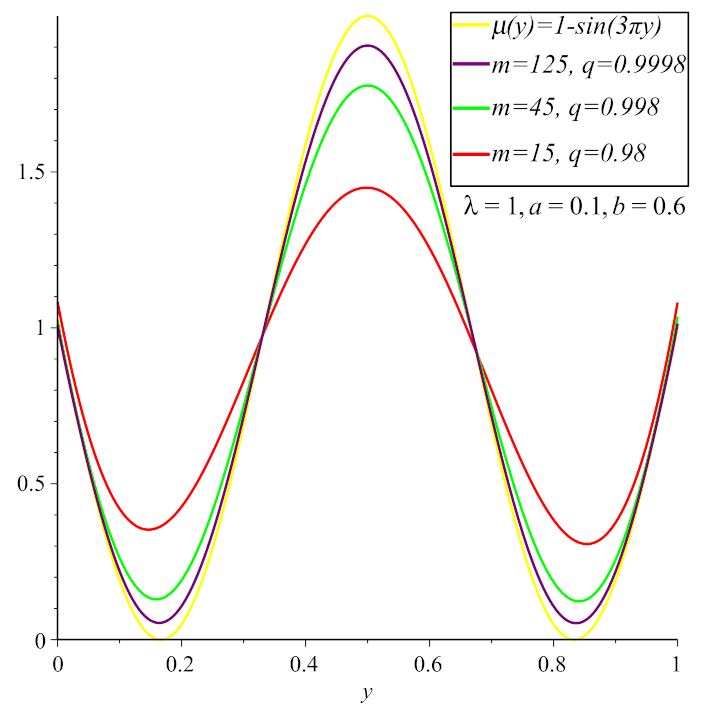
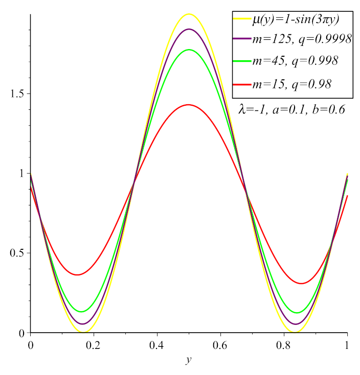
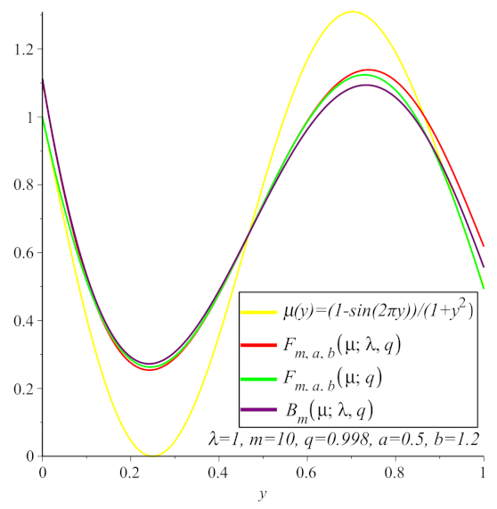
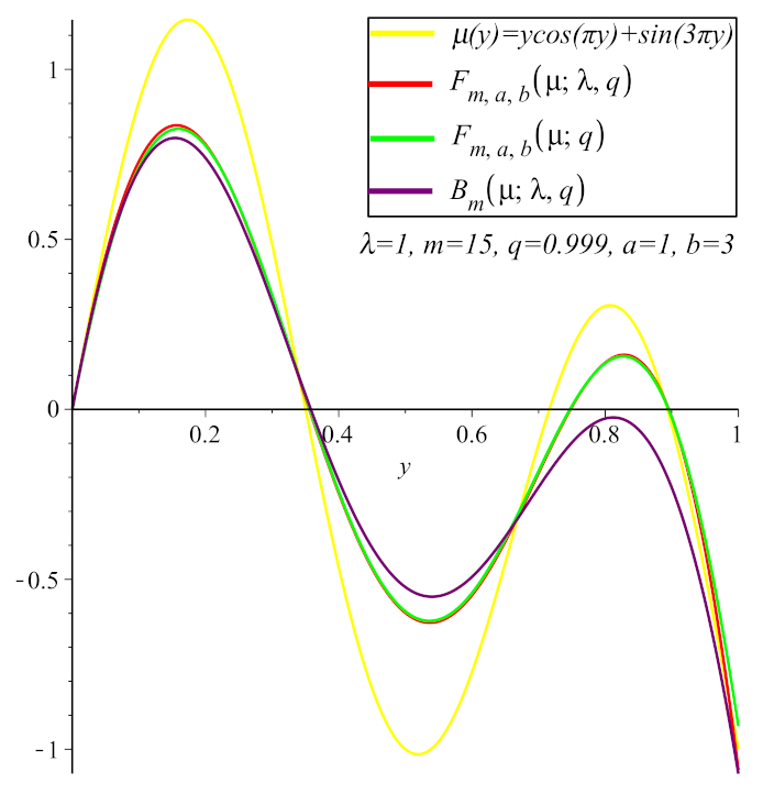
4. Graphs and Error Estimation Tables

In this section, in order to show the convergence behavior of the polynomials (4), we present some graphs and error of estimation tables for the different values of the $a,$ $b,$m, q, and $\lambda$ parameters. Furthermore, we compare the convergence of the polynomials (4) with (1) and (3) to the certain functions.

Example 1.

Let $\mu \left(y\right)=1-sin\left(3\pi y\right)$ $\left(yellow\right),$ $\lambda =1,$ $a=0.1$, and $b=0.6$. In Figure 1, we show the convergence of the polynomials (4) to $\mu \left(y\right)$ for $m=15,45,125$ $(red,green,purple)$ and $q\in (0,1]$. Furthermore, in Figure 2, we illustrate the convergence of the polynomials (4) to $\mu \left(y\right)$ for $\lambda =-1$, and the other parameters are the same as in Figure 1. In

Table 1. Error of approximation polynomials $F_{m,a,b}(\mu ;\lambda ,q,y)$ to $\mu \left(y\right)=1-sin\left(3\pi y\right)$ for $m=15,45,125$.

$\mathit{\lambda }$	q	$|\mathit{\mu }\left(\mathit{y}\right)-{\mathit{F}}_{\mathit{m},\mathit{a},\mathit{b}}(\mathit{\mu };\mathit{\lambda },\mathit{q},\mathit{y})|$		$\mathit{a}=0.1,\mathit{b}=0.6$
		$\mathit{m}=\mathbf{15}$	$\mathit{m}=\mathbf{45}$	$\mathit{m}=\mathbf{125}$
	0.98	0.550594325	0.306394389	0.213534145
1	0.998	0.504069181	0.222940932	0.094770016
	0.9998	0.499424268	0.215224376	0.085356093
	0.98	0.560196708	0.308330384	0.214499941
0	0.998	0.510708683	0.223434415	0.094830635
	0.9998	0.505790803	0.215616670	0.085380496
	0.98	0.569799091	0.310266384	0.215465740
−1	0.998	0.517348184	0.223927891	0.094891256
	0.9998	0.512157335	0.216008960	0.085404893

, we estimate the error of the approximation of the polynomials (4) to $\mu \left(y\right)$ with $a=0.1,$ $b=0.6,$ $-1\le \lambda \le 1$, $q\in (0,1]$, and $m=15,45,125,$ respectively. It is obvious from Table 1 that the absolute difference between the polynomials (4) and $\mu \left(y\right)$ becomes smaller as the value of m increases. Furthermore, in case $\lambda =1$, the polynomials (4) give better approximation results than in cases $\lambda =0$ and $\lambda =-1.$

Example 2.

Let $\mu \left(y\right)=(1-sin\left(2\pi y\right))/(1+y^2)$ $\left(yellow\right),$ $\lambda =1,$ $a=0.5$, $b=1.2$, and $q=0.998.$ In Figure 3, we show the convergence of the polynomials (4) $\left(red\right),$ (1) $\left(green\right),$ (3) $\left(purple\right)$ to $\mu \left(y\right)$ for $m=10$. In

Table 2. Error of approximation polynomials $F_{m,a,b}(\mu ;\lambda ,q,y)$, $F_{m,a,b}(\mu ;q,y)$, and $B_m(\mu ;\lambda ,y)$ to $\mu \left(y\right)=(1-sin\left(2\pi y\right)/(1+y^2)$ for $m=200$.

	$\mathit{q}=0.998$	$\mathit{a}=0.5$	$\mathit{b}=1.2$
y	$|\mathit{\mu }\left(\mathit{y}\right)-{\mathit{F}}_{\mathit{m},\mathit{a},\mathit{b}}(\mathit{\mu };\mathit{\lambda },\mathit{q},\mathit{y})|$	$|\mathit{\mu }\left(\mathit{y}\right)-{\mathit{F}}_{\mathit{m},\mathit{a},\mathit{b}}(\mathit{\mu };\mathit{q},\mathit{y})|$	$|\mathit{\mu }\left(\mathit{y}\right)-{\mathit{B}}_{\mathit{m}}(\mathit{\mu };\mathit{\lambda },\mathit{y})|$
0.1	0.0064703691	0.0066166279	0.0064908234
0.2	0.0178590518	0.0179015902	0.0179216560
0.3	0.0202453681	0.0202461350	0.0203259325
0.4	0.0098313720	0.0098337279	0.0098768282
0.5	0.0059935717	0.0060039098	0.0060271492
0.6	0.0166406345	0.0166436305	0.0167571955
0.7	0.0168553088	0.0168781498	0.0170138238
0.8	0.0094123445	0.0094737845	0.0095471335
0.9	0.0017028663	0.0017979154	0.0017552501

, we compare the convergence of the polynomials (4) with (3) and (1) to $\mu \left(y\right)$ for $a=0.5,$ $b=1.2,$ $\lambda =1$, $q=0.998$, and $m=200$. It is clear from Table 2 that the absolute difference between the polynomials (4) and $\mu \left(y\right)$ is smaller than (3) and $\mu \left(y\right)$ and (1) and $\mu \left(y\right)$. Namely, the polynomials (4) have a better approximation than the polynomials (3) and (1). One the other hand, from Table 2, one can check that, since $b-a<1$, then the polynomials (3) have a better approximation than (1).

Example 3.

Let $\mu \left(y\right)=ycos\left(\pi y\right)+sin\left(3\pi y\right)$ $\left(yellow\right),$ $\lambda =1,$ $a=1,$ $b=3$, and $q=0.999.$ In Figure 4, we demonstrate the convergence of the polynomials (4) $\left(red\right),$ (1) $\left(green\right),$ (3) $\left(purple\right)$ to $\mu \left(y\right)$ for $m=15$. In

Table 3. Error of approximation polynomials $F_{m,a,b}(\mu ;\lambda ,q,y)$, $F_{m,a,b}(\mu ;q,y)$, and $B_m(\mu ;\lambda ,y)$ to $\mu \left(y\right)=ycos\left(\pi y\right)+sin\left(3\pi y\right)$ for $m=150$.

	$\mathit{q}=0.99$	$\mathit{a}=1$	$\mathit{b}=25$
y	$|\mathit{\mu }\left(\mathit{y}\right)-{\mathit{F}}_{\mathit{m},\mathit{a},\mathit{b}}(\mathit{\mu };\mathit{\lambda },\mathit{q},\mathit{y})|$	$|\mathit{\mu }\left(\mathit{y}\right)-{\mathit{F}}_{\mathit{m},\mathit{a},\mathit{b}}(\mathit{\mu };\mathit{q},\mathit{y})|$	$|\mathit{\mu }\left(\mathit{y}\right)-{\mathit{B}}_{\mathit{m}}(\mathit{\mu };\mathit{\lambda },\mathit{y})|$
0.1	0.0395067635	0.0403109983	0.0421575117
0.2	0.0820586872	0.0820251352	0.0880156832
0.3	0.0404867906	0.0401846539	0.0436964312
0.4	0.0578630516	0.0580685817	0.0636539124
0.5	0.1098004706	0.1099528891	0.1228649275
0.6	0.0618640005	0.0620901607	0.0712086537
0.7	0.0266496768	0.0264485480	0.0327246974
0.8	0.0571950380	0.0572345301	0.0789298769
0.9	0.0166758581	0.0169176476	0.0381883355

, we compare the convergence of the polynomials (4) with (3) and (1) to $\mu \left(y\right)$ for $a=1,$ $b=25,$ $\lambda =1$, $q=0.99$, and $m=150$. It is clear from Table 3 that the absolute difference between the polynomials (4) and $\mu \left(y\right)$ is smaller than (3) and $\mu \left(y\right)$ and (1) and $\mu \left(y\right)$. As a result, our newly defined polynomials (4) have a better approximation than the polynomials (3) and (1). Further, from Table 2, one can check that, since $b-a>1$, then the polynomials (1) have a better approximation than the polynomials (3).

As a result, we observe from Figure 2, Figure 3 and Figure 4 and Table 2 and Table 3 that the proposed polynomials $F_{m,a,b}(\mu ;\lambda ,q,y)$ are the generalization of certain polynomials such as $(\lambda ,q)$-Bernstein $B_m(\mu ;\lambda ,y)$ [40] and generalized q-Bernstein polynomials $F_{m,a,b}(\mu ;q,y)$ [4]. The proposed polynomials have fewer errors of approximation if we change the related parameters, and they have better approximations.

5. Conclusions

In this research, we proposed and studied several approximation properties of generalized q-Bernstein polynomials based on Bernstein basis functions with shape parameter $\lambda \in [-1,1]$. We discussed a Korovkin-type convergence theorem, as well as the order of convergence concerning the usual modulus of continuity and Lipschitz-type functions. To make our research more intuitive, we considered some graphs and error estimation tables. As a result, the newly constructed polynomials (4) gave better approximation results than the previously studied polynomials (1) and (3) in terms of the values of some selected parameters. Because the shape parameter $\lambda$ is defined on the symmetric interval $[-1,1]$, there is more flexibility in constructing curves using this basis function, and at the same time, the corresponding linear polynomials with certain values of the shape parameter $\lambda$ have better convergence and more flexibility in approximating the related function class.

References

1. Lupaş, A. A q-analogue of the Bernstein operator. Semin. Numer. Stat. Calculus 1987, 9, 85–92. [Google Scholar]
2. Phillips, G.M. Bernstein polynomials based on the q-integers. Ann. Numer. Math. 1997, 4, 511–518. [Google Scholar]
3. Kac, V.; Cheung, P. Quantum Calculus; Springer Science & Business Media: Berlin/Heidelberg, Germany, 2001. [Google Scholar]
4. Karahan, D.; Izgi, A. On Approximation Properties of Generalized q-Bernstein Operators. Numer. Funct. Anal. Optim. 2018, 39, 990–998. [Google Scholar] [CrossRef]
5. Oruç, H.; Phillips, G.M. q-Bernstein polynomials and Bézier curves. J. Comput. Appl. Math. 2003, 151, 1–12. [Google Scholar] [CrossRef] [Green Version]
6. Mursaleen, M.; Khan, A. Generalized q-Bernstein-Schurer operators and some approximation theorems. J. Funct. Spaces. 2013, 2013, 1–7. [Google Scholar] [CrossRef]
7. Acar, T.; Aral, A. On pointwise convergence of q-Bernstein operators and their q-derivatives. Numer. Funct. Anal. Optim. 2015, 36, 287–304. [Google Scholar] [CrossRef]
8. Aslan, R.; İzgi, A. Some approximation results on modified q-Bernstein operators. J. Math. Anal. 2020, 11, 58–70. [Google Scholar]
9. Mahmudov, N.I. The moments for q-Bernstein operators in the case 0 < q < 1. Numer. Algorithms 2010, 53, 439–450. [Google Scholar]
10. Agratini, O. On certain q-analogues of the Bernstein operators. Carpathian J. Math. 2008, 281–286. [Google Scholar]
11. Ghomanjani, F.; Shateyi, S. A new approach for solving Bratu’s problem. Demonstr. Math. 2019, 52, 336–346. [Google Scholar] [CrossRef]
12. Mohiuddine, S.A.; Ahmad, N.; Özger, F.; Hazarika, B. Approximation by the parametric generalization of Baskakov-Kantorovich operators linking with Stancu operators. Iran J. Sci. Technol. Trans. Sci. 2021, 45, 593–605. [Google Scholar] [CrossRef]
13. Alotaibi, A.; Özger, F.; Mohiuddine, S.A.; Alghamdi, M.A. Approximation of functions by a class of Durrmeyer–Stancu type operators which includes Euler’s beta function. Adv. Differ. Equ. 2021, 2021, 13. [Google Scholar] [CrossRef]
14. Mursaleen, M.; Ansari, K.J.; Khan, A. Approximation properties and error estimation of q-Bernstein shifted operators. Numer. Algorithms 2019, 84, 1–21. [Google Scholar] [CrossRef]
15. Khan, W.A.; Khan, I.A.; Duran, U.; Acikgoz, M. Apostol type (p,q)-Frobenius–Eulerian polynomials and numbers. Afr. Mat. 2021, 32, 115–130. [Google Scholar] [CrossRef]
16. Kang, J.Y.; Khan, W.A. A new class of q-Hermite-based Apostol type Frobenius Genocchi polynomials. Commun. Korean Math. Soc. 2020, 35, 759–771. [Google Scholar]
17. Khan, W.A.; Nisar, K.S.; Baleanu, D. A note on (p,q)-analogue type of Fubini numbers and polynomials. AIMS Math. 2020, 5, 2743–2757. [Google Scholar] [CrossRef]
18. Farouki, R.T. The Bernstein polynomial basis: A centennial retrospective. Comput. Aided Geometr. Design 2012, 29, 379–419. [Google Scholar] [CrossRef]
19. Khan, K.; Lobiyal, D.K. Bézier curves based on Lupaş (p,q)-analogue of Bernstein functions in CAGD. J. Comput. Appl. Math. 2017, 317, 458–477. [Google Scholar] [CrossRef]
20. Khan, K.; Lobiyal, D.K.; Kılıçman, A. Bézier curves and surfaces based on modified Bernstein polynomials. Azerb. J. Math. 2019, 9, 3–21. [Google Scholar]
21. Farin, G. Curves and Surfaces for Computer-Aided Geometric Design: A Practical Guide; Elsevier: Amsterdam, The Netherlands, 2014. [Google Scholar]
22. Sederberg, T.W. Computer Aided Geometric Design. 2012. Available online: https://scholarsarchive.byu.edu/facpub/1/ (accessed on 1 September 2021).
23. Ye, Z.; Long, X.; Zeng, X.M. Adjustment algorithms for Bézier curve and surface. In Proceedings of the International Conference on 5th Computer Science and Education, Hefei, China, 24–27 August 2010. [Google Scholar]
24. Cai, Q.-B.; Zhou, G.; Li, J. Statistical approximation properties of λ-Bernstein operators based on q-integers. Open Math. 2019, 17, 487–498. [Google Scholar] [CrossRef]
25. Acu, A.M.; Manav, N.; Sofonea, D.F. Approximation properties of λ-Kantorovich operators. J. Inequal. Appl. 2018, 2018, 202. [Google Scholar] [CrossRef] [PubMed] [Green Version]
26. Srivastava, H.M.; Özger, F.; Mohiuddine, S.A. Construction of Stancu-type Bernstein operators based on Bézier bases with shape parameter λ. Symmetry 2019, 11, 316. [Google Scholar] [CrossRef] [Green Version]
27. Özger, F. Applications of generalized weighted statistical convergence to approximation theorems for functions of one and two variables. Numer. Funct. Anal. Optim. 2020, 41, 1990–2006. [Google Scholar] [CrossRef]
28. Mursaleen, M.; Al-Abied, A.A.H.; Salman, M.A. Chlodowsky type (λ,q)-Bernstein-Stancu operators. Azerb. J. Math. 2020, 10, 75–101. [Google Scholar]
29. Rahman, S.; Mursaleen, M.; Acu, A.M. Approximation properties of λ-Bernstein-Kantorovich operators with shifted knots. Math. Meth. Appl. Sci. 2019, 42, 4042–4053. [Google Scholar] [CrossRef]
30. Cai, Q.-B.; Lian, B.Y.; Zhou, G. Approximation properties of λ-Bernstein operators. J. Inequal. Appl. 2018, 2018, 61. [Google Scholar] [CrossRef] [PubMed]
31. Özger, F. Weighted statistical approximation properties of univariate and bivariate λ-Kantorovich operators. Filomat 2019, 33, 3473–3486. [Google Scholar] [CrossRef]
32. Özger, F. On new Bézier bases with Schurer polynomials and corresponding results in approximation theory. Commun. Fac. Sci. Univ. Ank. Ser. A1 Math. Stat. 2020, 69, 376–393. [Google Scholar] [CrossRef]
33. Aslan, R. Some approximation results on λ-Szasz-Mirakjan-Kantorovich operators. FUJMA. 2021, 4, 150–158. [Google Scholar]
34. Özger, F.; Srivastava, H.M.; Mohiuddine, S.A. Approximation of functions by a new class of generalized Bernstein-Schurer operators. Rev. R. Acad. Cienc. Exactas Fís. Nat. Ser. A Math. RACSAM 2020, 114, 173. [Google Scholar] [CrossRef]
35. Mohiuddine, S.A.; Özger, F. Approximation of functions by Stancu variant of Bernstein-Kantorovich operators based on shape parameter α. Rev. R. Acad. Cienc. Exactas Fís. Nat. Ser. A Math. RACSAM 2020, 114, 70. [Google Scholar] [CrossRef]
36. Srivastava, H.M.; Ansari, K.J.; Özger, F.; Ödemiş Özger, Z. A link between approximation theory and summability methods via four-dimensional infinite matrices. Mathematics 2021, 9, 1895. [Google Scholar] [CrossRef]
37. Özger, F.; Demirci, K.; Yıldız, S. Approximation by Kantorovich variant of λ-Schurer operators and related numerical results. In Topics in Contemporary Mathematical Analysis and Applications; CRC Press: Boca Raton, FL, USA, 2020; pp. 77–94. ISBN 9780367532666. [Google Scholar]
38. Cai, Q.-B.; Torun, G.; Dinlemez Kantar, Ü. Approximation Properties of Generalized λ-Bernstein-Stancu-Type Operators. J. Math. 2021, 2021, 5590439. [Google Scholar] [CrossRef]
39. Ghomanjani, F.; Farahi, M.H.; Kılıçman, A.; Kamyad, A.V.; Pariz, N. Bezier curves based numerical solutions of delay systems with inverse time. Math. Probl. Eng. 2014, 2014, 602641. [Google Scholar] [CrossRef]
40. Cai, Q.-B.; Cheng, W.T. Convergence of λ-Bernstein operators based on (p,q)-integers. J. Inequal. Appl. 2020, 2020, 35. [Google Scholar] [CrossRef] [Green Version]
41. Micchelli, C. The saturation class and iterates of Bernstein polynomials. J. Approx. Theory 1973, 8, 1–18. [Google Scholar] [CrossRef] [Green Version]
42. Campiti, M. Convergence of iterated Boolean-type sums and their iterates. Numer. Funct. Anal. Optim. 2018, 39, 1054–1063. [Google Scholar] [CrossRef]
43. Occorsio, D.; Russo, M.G.; Themistoclakis, W. Some numerical applications of generalized Bernstein operators. Constr. Math. Anal. 2021, 4, 186–214. [Google Scholar]
44. Izgi, A. Approximation by a class of new type Bernstein polynomials of one and two variables. Glob. J. Pure Appl. Math. 2012, 8, 55–71. [Google Scholar]
45. Korovkin, P.P. On convergence of linear positive operators in the space of continuous functions. Dokl. Akad. Nauk SSSR. 1953, 90, 961–964. [Google Scholar]
46. Altomare, F.; Campiti, M. Korovkin-Type Approximation Theory and Its Applications; Walter de Gruyter: Berlin, Germany, 2011; Volume 17. [Google Scholar]
Figure 1. The convergence of polynomials F m , a , b ( μ ; λ , q , y ) to μ ( y ) = 1 sin ( 3 π y ) ( y e l l o w ) for m = 15 ( r e d ) , m = 45   ( g r e e n ) , m = 125 ( p u r p l e ) , and λ = 1 .
Symmetry 13 01919 g001
Figure 2. The convergence of polynomials F m , a , b ( μ ; λ , q , y ) to μ ( y ) = 1 sin ( 3 π y ) ( y e l l o w ) for m = 15 ( r e d ) , m = 45   ( g r e e n ) , m = 125 ( p u r p l e ) , and λ = 1 .
Symmetry 13 01919 g002
Figure 3. The convergence of polynomials F m , a , b ( μ ; λ , q , y ) ( r e d ) ,   F m , a , b ( μ ; q , y ) ( g r e e n ) , and B m ( μ ; λ , y ) ( p u r p l e ) to μ ( y ) = ( 1 sin ( 2 π y ) ) / ( 1 + y 2 ) ( y e l l o w ) for m = 10 .
Symmetry 13 01919 g003
Figure 4. The convergence of polynomials F m , a , b ( μ ; λ , q , y ) ( r e d ) ,   F m , a , b ( μ ; q , y ) ( g r e e n ) , and B m ( μ ; λ , y ) ( p u r p l e ) to μ ( y ) = y cos ( π y ) + sin ( 3 π y ) ( y e l l o w ) for m = 15 .
Symmetry 13 01919 g004