A Symmetric Controllable Hyperchaotic Hidden Attractor

Abstract

By introducing a simple feedback, a hyperchaotic hidden attractor is found in the newly proposed Lorenz-like chaotic system. Some variables of the equilibria-free system can be controlled in amplitude and offset by an independent knob. A circuit experiment based on Multisim is consistent with the theoretic analysis and numerical simulation.

1. Introduction

As we all know, chaos is ubiquitous in nature and human society, and has great potential in engineering applications. However, there exists great challenge in conditioning broadband chaotic signals, and appropriate amplitude and polarity are the key specifications for chaos generation and transmission [1,2,3], and therefore, recently great efforts have been made on the research of amplitude control and offset boosting. Normally, the amplitude of system variable requires further adjusting a couple of parameters. In many cases, a unipolar signal is more suitable for transmitting in inter-coupled integrated circuits. Such a challenge exists in the conversion from the bipolar signal to unipolar signal. An independent non-bifurcation parameter to rescale the signal without revising the Lyapunov exponents is important for chaos application. Suitable signal control saves the modulator in chaos-based applications [4,5], including amplitude control [6,7] and offset boosting [8,9].

In addition, hidden attractors exist in chaos, but one cannot find them from the neighborhood of any equilibrium point. Thus, it is of great value in theoretical and physical significance and engineering application to study the realization method of hidden attractors. The Chua system, Lorenz-like systems, and the chaotic systems with stable equilibria [10,11,12,13,14,15], line equilibria [16,17,18], or no equilibria [19,20,21,22,23,24] give us impressive points. Hyperchaos with higher complexity is beneficial to secure communication, so some research extends to hyperchaos. A hyperchaotic system with a hidden attractor was proposed by Wang et al. [25]; Chlouverakis and Sprott [26] claimed the simplest hyperchaotic snap system in algebra; and Yuan et al. [27] showed a memristive multi-scroll hyperchaotic system. Other many hyperchaotic systems have come out of the Lorenz-like system [28,29,30,31]. Some other hyperchaotic ones have been proposed, including a memristive hyperchaotic system [32,33], fractional order hyperchaotic system [34,35] or hyperchaotic multi-wing system [36,37]. To the best of our knowledge, there is no relevant research on a hyperchaotic hidden attractor with geometric control. Based on a three-dimensional Lorenz-like system, Wang et al. [38] put forward a hyperchaotic system for producing multi-wing attractors; while in this work, the proposed system has four features as follows:

I)

There exists a parameter to control amplitude and frequency of signals in a small range.

II)

Amplitude of x and y can be controlled simultaneously.

III)

There is an offset boosting controller.

IV)

A special parameter can realize both amplitude and offset control of one system variable.

As shown in Figure 1, the proposed hyperchaotic system has multiple independent geometric controllers including controllers for rescaling amplitude, frequency and offset. Some of the reported 4-D hyperchaotic Lorenz-like systems are listed in Table 1. In the paper, the system controllers are signal controllers and multistability observers as well. In Section 2, the mathematical model of the hyperchaotic system is given. In Section 3, complex dynamic behavior is analyzed. The process of amplitude control and offset boosting is discussed in Section 4. In Section 5, multistability is investigated. In Section 6, the analog circuit is given. Finally, we give the conclusions and discussion.

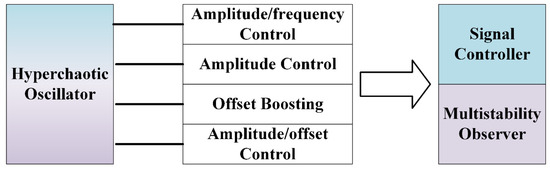
Figure 1. Hyperchaotic attractor with multiple independent controllers.

Table 1. Comparison of the Lorenz-like hyperchaotic systems.

Reference	Number of Terms	Number of Equilibrium	Amplitude/Frequency Control	Amplitude/Offset Control
[15]	9	one	no	not mentioned
[28]	10	line equilibrium	no	not mentioned
[30]	10	one	no	not mentioned
[31]	9	one	no	not mentioned
[38]	9	no	no	not mentioned
this work	9	no	yes	yes

2. Model Description

A 3-D Lorenz-like chaotic system is proposed by Cang et al [39], which is,

$$\{\begin{array}{l}\dot{x}=-ay-xz,\\ \dot{y}=-x+xz,\\ \dot{z}=-d-xy.\end{array}$$

(1)

System (1) has a simple rotational symmetric structure with six terms. Based on system (1), a new hyperchaotic system is proposed as,

$$\{\begin{array}{l}\dot{x}=-ay-xz-u,\\ \dot{y}=-cx+xz,\\ \dot{z}=-b-mxy,\\ \dot{u}=kx-y.\end{array}$$

(2)

where x, y, z, u are system variables, and a, b, c, k are bifurcation parameters of system (2). When a = 5, b = 4, c = 1, k = 0.5 and m = 1, system (2) has a hyperchaotic attractor with Lyapunov exponents (0.3606, 0.1222, 0, −1.4827) and a Kaplan-Yorke dimension of D_KY = 3.3256 under initial conditions (1, −1, −1, 1), as shown in Figure 2.

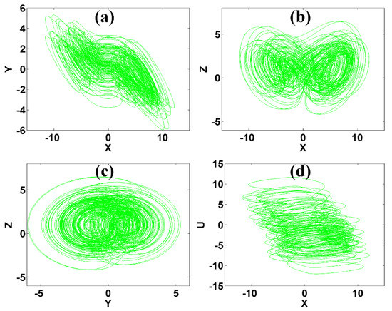
Figure 2. Hyperchaotic attractor of system (2) with a = 5, b = 4, c = 1, k = 0.5, m = 1 and initial conditions [1, −1, −1, 1]: (a) x-y plane, (b) x-z plane, (c) y-z plane, (d) x-u plane.

The hyper-volume contraction is

$$\nabla V=\frac{\partial \dot{x}}{\partial x}+\frac{\partial \dot{y}}{\partial y}+\frac{\partial \dot{z}}{\partial z}+\frac{\partial \dot{u}}{\partial u}=-z$$

(3)

When a = 5, b = 4, c = 1 and k = 0.5, the dissipative curve of Equation (3) is as shown in Figure 3. The negative average of $\nabla V$ proves that system (2) is dissipative.

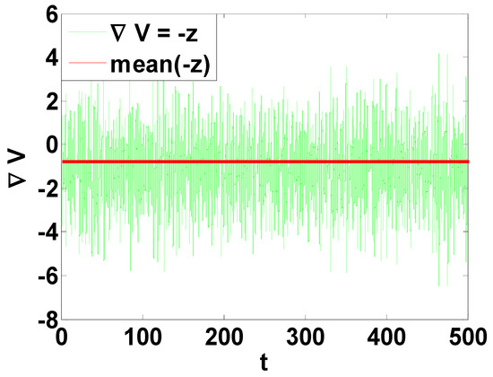
Figure 3. Dissipative curve of system (2).

3. Basic Dynamic Analysis

3.1. Anylis of Equilibria

For system (2), the equilibria can be solved by the following equation:

$$\{\begin{array}{l}-ay-xz-u=0\\ -cx+xz=0\\ -b-mxy=0\\ kx-y=0\end{array}$$

(4)

The fourth equation indicates that $y=kx$, but the third equation means that $b=-mxy$, then b = −mkx², which means that there is no real solution, correspondingly the hyperchaotic attractor of system (2) is hidden.

3.2. Bifurcation Analysis

For system (2), the parameters modify the dynamics effectively. To make the demonstration simpler, we ignore the multistability caused by the special structure of symmetry. When b = 4, c = 1, k = 0.5, m = 1 under initial conditions (1, −1, −1, 1), Lyapunov exponent spectra and bifurcation diagram when a varies in [−10, 23.4] are shown in Figure 4, where a typical transition from period to chaos shows up and finally system (1) results in the state of hyperchaos. Typical phase trajectories are shown in Figure 5. Quasi-periodicity was not found in the examination interval of system (2). When a = 5, c = 1, k = 0.5, m = 1 and initial conditions are (1, −1, −1, 1), when b varies in [0, 15], system (2) heads to hyperchaos from chaos. Lyapunov exponent spectra and bifurcation diagrams are shown in Figure 6, which shows a robust hyperchaos. Both cases have almost linearly scaled Lyapunov exponents in specific regions indicating the function of frequency rescaling.

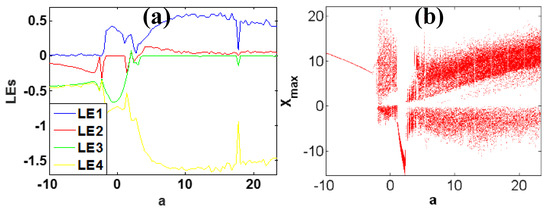
Figure 4. Dynamical behavior of system (2) with b = 4, c = 1, k = 0.5, m = 1 under initial conditions [1, −1, −1, 1]: (a) Lyapunov exponents, (b) bifurcation diagram.

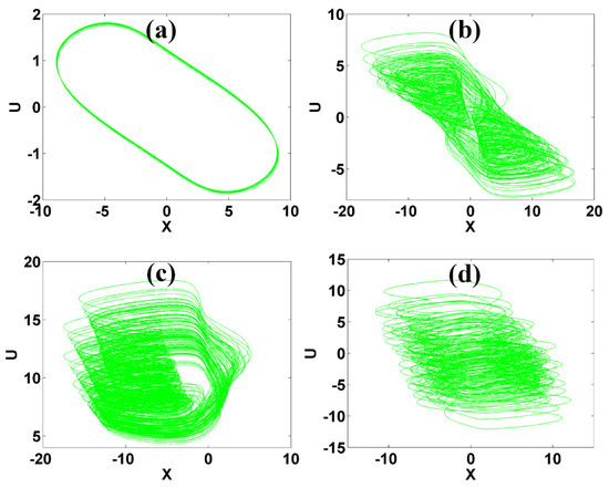
Figure 5. Typical phase trajectories of system (2) with b = 4, c = 1, k = 0.5, m = 1 under initial condition [1, −1, −1, 1] in the plane x-u: (a) a = −5 (period), (b) a = −0.6 (chaos), (c) a = 3 (chaos), (d) a = 5 (hyperchaos).

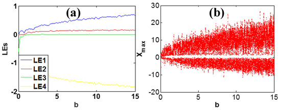
Figure 6. Dynamical behavior of system (2) with a = 5, c = 1, k = 0.5, m = 1under initial condition [1, −1, −1, 1]: (a) Lyapunov exponents, (b) bifurcation diagram.

Comparing Figure 4 and Figure 6, we can see that the parameter a or b visits chaos quickly but modifies the solution in its own way. The parameter a almost has positive correlation with amplitude in a limited range. Meanwhile parameter b has positive correlation with amplitude and frequency, which is distinct and different from other systems. Typical phase trajectories and waveforms are shown in Figure 7.

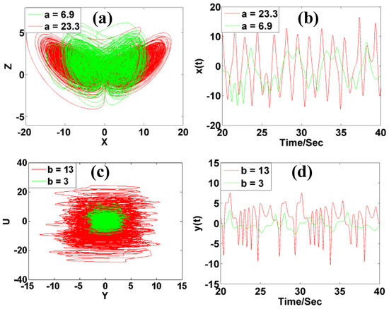
Figure 7. Chaotic oscillations of system (2) with c = 1, k = 0.5, m = 1 under initial condition [1, −1, −1, 1]: (a) phase trajectory in x-z (b = 4), (b) signal x(t), (c) phase trajectory in y-u plane (a = 5), (d) signal y(t).

Fix the parameters a = 5, b = 4, k = 0.5, m = 1, when parameter c varies in [0, 1.7]; the Lyapunov exponent spectra and bifurcation diagram are shown in Figure 8a,b. When c varies in [0, 1.4], system (2) exhibits hyperchaos, while when c varies in [1.4, 1.7], system (2) presents chaos. When a = 5, b = 4, c = 1 and m = 1, the parameter k varies in [0.15, 7.8]; the Lyapunov exponent spectra and bifurcation diagram are shown in Figure 8c,d. When k varies in [0.15, 1.82], system (2) keeps chaos, and when c varies in [1.82, 7.8], system (2) exhibits hyperchaos. Comparing the Lyapunov exponents controlled by parameters c and k, system (2) has relatively robust hyperchaos under the parameters c.

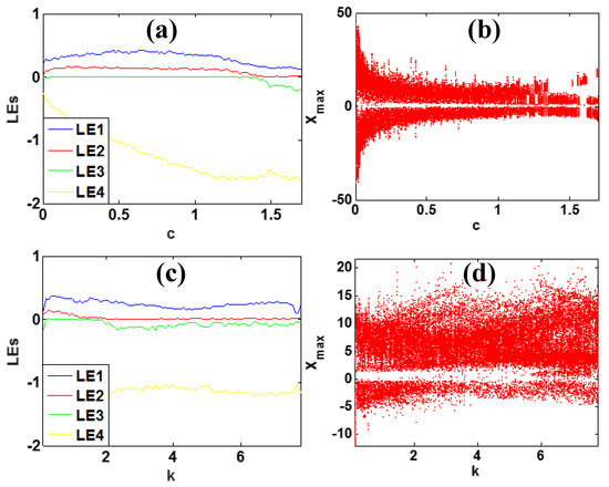
Figure 8. Dynamical behavior of system (2) with a = 5, b = 4, m = 1 under initial conditions [1, −1, −1, 1]: (a,b): Lyapunov exponents and bifurcation diagram of c when k = 0.5, (c,d): Lyapunov exponents and bifurcation diagram of k when c = 1.

3.3. Amplitude Control

Besides the above two control knobs, the parameter m in the third dimension in system (2) is a single non-bifurcation knob for amplitude control. To understand this rescaling mechanism, we turn back to the initial system (2). Here, we take the transformation: $x\to hx,y\to hy,z\to z,$ $u\to hu(h>0)$, which only leaves an additional coefficient in the third dimension:

$$\{\begin{array}{l}\dot{x}=-ay-xz-u,\\ \dot{y}=-cx+xz,\\ \dot{z}=-b-m{h}^{2}xy,\\ \dot{u}=kx-y.\end{array}$$

(5)

indicating that the amplitude of variables x, y and u can be controlled by the parameter m, with the signal z unchanged. It also has no effect on the frequency of the hyperchaotic chaotic signals.

The output signals are controlled by the non-bifurcation parameter m in system (2). As shown in Figure 9, the amplitude of the signals x, y and u are rescaled by the non-bifurcation parameter m. When m = 0.25, the amplitudes of the x, y and u signals are very large. The amplitudes of the x, y and u signals decrease with an inverse proportion to the parameter m without changing the amplitude of z. Figure 10 shows the phase trajectories on the planes of x-u and y-z when the control parameter m varies.

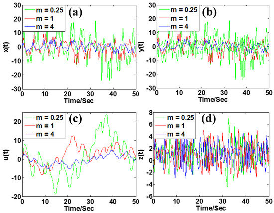
Figure 9. Rescaled variables in system (2) with a = 5, b = 4, c = 1, k = 0.5 under initial condition [1, −1, −1, 1]: (a) signal x(t), (b) signal y(t), (c) signal u(t), (d) signal z(t).

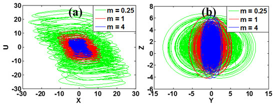
Figure 10. Phase trajectories of system (2) with a = 5, b = 4, c = 1, k = 0.5 under initial condition [1, −1, −1, 1]: (a) x-u, (b) y-z.

As we can see in Figure 11a, when the parameter m varies in [0, 5], the average of the absolute values of state variables x, y and u significantly decreases with an inverse proportion to m, while the average of signal z basically has no change. The corresponding Lyapunov exponent spectrum of parameter m varies in [0, 5] are shown in Figure 11b. It can be further proved that the parameter m of system (2) does not change the frequency of the signals.

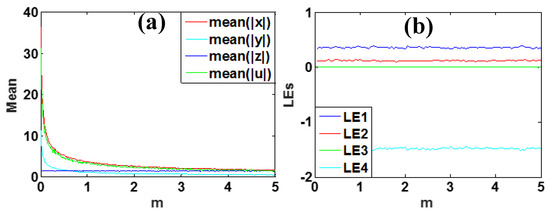
Figure 11. Dynamical evolution of system (2) with a = 5, b = 4, c = 1, k = 0.5 and initial condition [1, −1, −1, 1]: (a) average values of the absolute value of chaotic signals, (b) invariable Lyapunov exponents.

3.4. Offset Boosting

Since the derivative of a constant is zero, when a constant is added to a variable in a dynamical system, the system exhibits the same dynamics. To understand this, we turn back to the initial system (2). Here, we take the transformation: $u\to u-n$, which does not change the system equation but only leaves an additional constant in the first equation:

$$\{\begin{array}{l}\dot{x}=-ay-xz-u+n,\\ \dot{y}=-cx+xz,\\ \dot{z}=-b-mxy,\\ \dot{u}=kx-y.\end{array}$$

(6)

When changing the variable u with $u-n$ (n is a constant), system (2) gives the same dynamics. Therefore, if the variable u does not show in the other equations in system (2), the introduced constant will give a boosting control of the variable u. The chaotic signal u(t) can be revised from unipolar to bipolar or vice versa.

When a = 5, b = 4, c = 1, k = 0.5 and m = 1, the signal u is boosted from a bipolar to a unipolar one, which is indicated by the red and blue attractors in Figure 12a. The waveform of chaotic signal u(t) is shown in Figure 12b. The change of parameter n causes the up and down translation of the signal u(t). Some monostable systems have relatively large areas of basins of attraction; therefore, the initial conditions do not need to modify according to the variable which makes the offset control simpler, as shown in Figure 13.

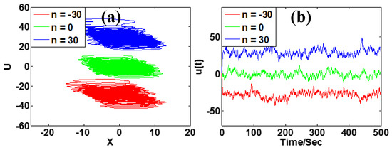
Figure 12. Typical chaotic oscillation of system (6) with a = 5, b = 4, c = 1, k = 0.5, m = 1 under initial condition [1, −1, −1, 1]: (a) phase trajectory in the plane of x-u, (b) waveform u(t).

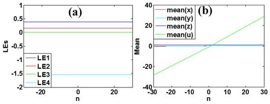
Figure 13. Dynamical evolution of system (6) with a = 5, b = 4, c = 1, k = 0.5, m = 1 under initial conditions [1, −1, −1, 1]: (a) Lyapunov exponent spectra of n, (b) average values of the hyperchaotic signal.

Here the offset of the variable u is boosted along the u-axis according to the constant n. When n is positive, u is moved in the positive direction, and negative n causes the opposite direction. When the boosting controller n is changed from −30 to 30, system (6) has the same Lyapunov exponents, which is shown in Figure 13. The average value of variable u changes linearly with the increase of parameter n, while others remain unchanged.

3.5. Mixed Geometric Control

More striking, parameter c almost has a positive correlation with the offset of signal z, almost without changing other signals, and also has a negative correlation with the amplitude of variable x and positive correlation with the amplitude of variable y. Figure 14 shows the typical phase trajectories and waveforms. Figure 15 shows the corresponding Lyapunov exponent spectra and average value of the x, y and z signals. Therefore, all in all, there are five parameters, a, b, c, m and n, rescaling the system variables, some of which are restricted in a specific region, as shown in Table 2.

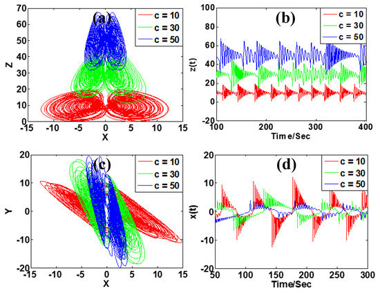
Figure 14. Typical chaotic oscillation of system (2) with a = 5, b = 4, k = 0.5, m = 1 under initial conditions [1, −1, −1, 1]: (a) phase trajectory in x-z, (b) signal z(t), (c) phase trajectory in x-y, (d) signal x(t).

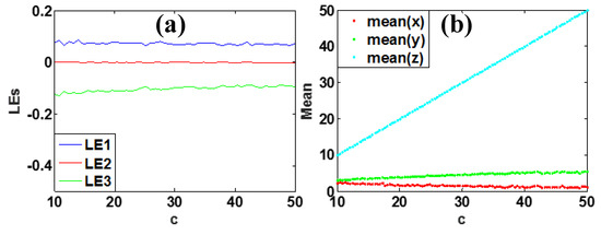
Figure 15. Dynamical evolution of system (2) with a = 5, b = 4, k = 0.5, m = 1 under initial conditions [1, −1, −1, 1]: (a) Lyapunov exponent spectra of c, (b) average values of the signals x, y and z.

Table 2. Five independent parameters in system (2) for geometric control.

Parameters	Execution Interval	Amplitude Control	Frequency Control	Offset Control
a	[6.9, 23.3]	positive control with x	positive	no
b	[3, 13]	positive control with x, y, z, u	positive	no
c	[10, 50]	positive control with y negative control with x	no	z
m	[0.1, 5]	Positive control with x, y, u	no	no
n	[−30, 30]	no	no	u

4. Bistability Analysis

In all the above analysis, we did not consider the multistability in each issue to simplify the demonstration. In fact, for the special structure of symmetry, coexisting attractors exist in their own basins of attraction in phase space. Specifically, for symmetrical systems, when the symmetry is broken, a pair of symmetrical coexisting attractors usually show up.

System (2) is a rotational symmetric system, which can be proved by the invariance of transformation $x\to -x,y\to -y,z\to z,u\to -u$. Symmetric systems are prone to show multistability due to the effect of broken symmetry. In general, predicting multistability seems not easy in theory. A common method to identify multistability is using the basins of attraction based on the ergodic initial conditions. Alternative methods can resort to non-bifurcation manipulation, in which a linear transformation is performed on the basin of attraction to generate a dynamical dispersion for a fixed initial condition, which can reveal different coexisting symmetrical pairs by generating different average values [40].

When offset boosting is introduced from the variables x and u,

$$\{\begin{array}{l}\dot{x}=-ay-(x+d)z-(u-d),\\ \dot{y}=(z-c)(x+d),\\ \dot{z}=-b-m(x+d)y,\\ \dot{u}=k(x+d)-y.\end{array}$$

(7)

and the average values of variables x and u will change according to the offset control parameter d. The coexisting attractors are drawn into different areas of the basin since the basins of attraction of the coexisting symmetric pair of attractors also change according to the offset parameter, as shown in Figure 16. In Figure 16a, the averages of variables x and u are revised by the offset parameters, while the average values of variable y remains the same. From Figure 16b, the invariance of Lyapunov exponents indicates the same structure of the symmetric pair of coexisting attractors. The typical phase trajectories of the symmetrical attractors of the system (2) under a pair of opposite initial conditions are shown in Figure 17.

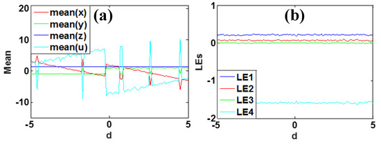
Figure 16. Dynamical behaviors of system (7) with a = 5, b = 4, k = 0.5, m = 1 and initial condition [1, −1, −1, 1], when parameter d varies in [−5, 5]: (a) average values of the signals, (b) Lyapunov exponents.

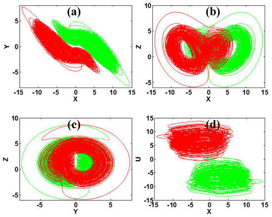
Figure 17. Coexisting symmetrical chaotic attractors of system (2) with a = 5, b = 4, c = 1.3, k = 0.5, m = 1 with initial conditions IC1 = (1, −1, −1, 1) (green); IC2 = (−1, 1, −1, −1) (red).

To further verify the multistability in system (2), the basin of attraction is shown in Figure 18, which has the predicted symmetry and complex fractal structure. To show the types of attractors more clearly and comprehensively, the similar chaotic attractors are presented using an identical color in the basin of attraction. It can be clearly seen that there are two areas in different colors in the basin. The corresponding Lyapunov exponents of the two attractors are (0.2137, 0.0623, 0, -1.5761), and the Kaplan-Yorke dimension is 3.1751.

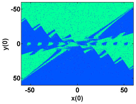
Figure 18. Basins of attraction of system (2) with a = 5, b = 4, c = 1.3, k = 0.5, m = 1 in plane of z(0) = −1 and u(0) = 0.

Both chaotic and hyperchaotic attractors show sensitivity to the initial condition, and furthermore, multistability and hyperchaos make the sensitivity more complicated. From two initial conditions in the same basin of attraction, even a slight difference results in great divergence in system (2), which is shown in Figure 19a. While from the two initial conditions in different basins of attraction, the slight difference leads to two separate phase trajectories, as shown in Figure 19b.

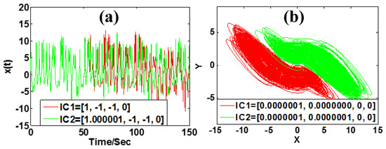
Figure 19. Dynamical behavior of system (2) with a = 5, b = 4, k = 0.5, m = 1 under different initial condition (a) c = 1; (b) c = 1.3.

5. Circuit Implementation

The analog circuit of system (2) is designed as shown in Figure 20 with the circuit equation:

$$\{\begin{array}{l}\dot{x}=-\frac{1}{R_1{C}_1}y-\frac{1}{R_2{C}_1}xz-\frac{1}{R_3{C}_1}u\\ \dot{y}=-\frac{1}{R_4{C}_2}x+\frac{1}{R_5{C}_2}xz\\ \dot{z}=-\frac{1}{R_6{C}_3}+\frac{1}{R_7{C}_3}xy\\ \dot{u}=\frac{1}{R_8{C}_4}x-\frac{1}{R_9{C}_4}y\end{array}$$

(8)

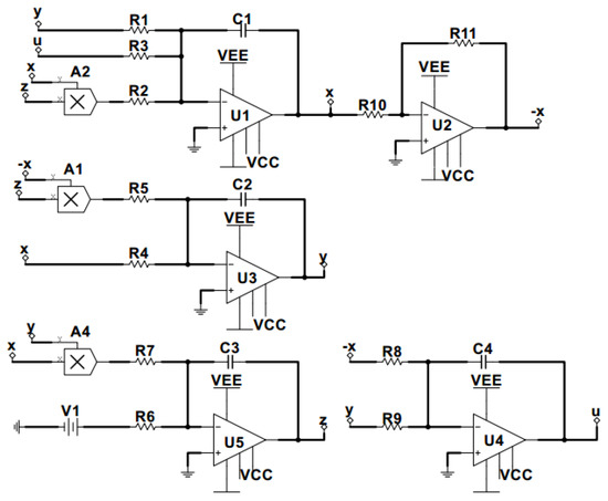
Figure 20. Circuit schematic of system (8).

Totally, the hyperchaotic circuit consists of four channels, which contain the integration, addition, subtraction, and nonlinear operations. The circuit is powered by 18V. The variables x, y, z and u in system (2) are the state voltages of the capacitors in four channels. The corresponding circuit element parameters can be selected as $C_1=C_2=C_3=C_4=10nF$, $R_2=R_5=R_7=4k\Omega$, $R_3=R_4=R_9=40k\Omega$, $R_1=8k\Omega$, $R_6=100k\Omega ,R_8=80k\Omega ,R_{10}=R_{11}=10k\Omega$. Here, a common time scale of 1000 is applied for better demonstration in the oscilloscope. The phase trajectories in circuit (8) under amplitude control are shown in Figure 21. Circuit experiment proves that the parameter m rescales the amplitude of x, y and u. Symmetric attractors are shown in Figure 22.

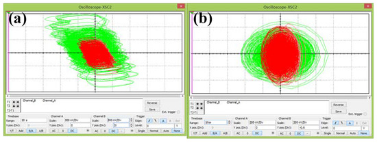
Figure 21. Circuit simulation of system (8) with a = 5, b = 4, c = 1.3, k = 0.5, m = 1 (green), m = 4 (red) under initial condition [1, −1, −1, 1]: (a) x-u plane, (b) y-z plane.

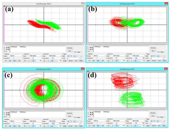
Figure 22. Circuit simulation of symmetric attractors in system (8) with a = 5, b = 4, c = 1.3, k = 0.5, m = 1 under initial conditions IC1= (1, −1, −1, 1)(green), IC2= (−1, 1, −1, −1)(red): (a) x-y plane, (b) x-z plane, (c) y-z plane, (d) x-u plane.

6. Discussion and Conclusions

A hidden hyperchaotic attractor is found, which has the property of amplitude control and offset boosting. The proposed system shares a symmetric structure, where one can find an independent knob for amplitude control. An extra introduced dimension leaves an opportunity for attractor shifting in phase space by an independent controller. Broken symmetry induced bistability is also well addressed in this work. All the coexisting symmetric attractors governed by the basin of attraction can be rescaled by the non-bifurcation parameter. Numerical and circuit simulation agree with each other proving the properties found in the hyperchaotic system.

References

- Li, C.; Sprott, J.C. Amplitude control approach for chaotic signals. Nonlinear Dyn. 2013, 73, 1335–1341. [Google Scholar] [CrossRef]
- Li, C.; Sprott, J.C. Finding coexisting attractors using amplitude control. Nonlinear Dyn. 2014, 78, 2059–2064. [Google Scholar] [CrossRef]
- Chen, H.; Bayani, A.; Akgul, A.; Jafari, M.-A.; Pham, V.-T.; Wang, X.; Jafari, S. A flexible chaotic system with adjustable amplitude, largest Lyapunov exponent, and local Kaplan–Yorke dimension and its usage in engineering applications. Nonlinear Dyn. 2018, 92, 1791–1800. [Google Scholar] [CrossRef]
- Wang, C.; Liu, X.; Xia, H. Multi-piecewise quadratic nonlinearity memristor and its 2N-scroll and 2N + 1-scroll chaotic attractors system. Chaos Interdiscip. J. Nonlinear Sci. 2017, 27, 033114. [Google Scholar] [CrossRef] [PubMed]
- Hu, W.; Akgul, A.; Li, C.; Zheng, T.; Li, P. A switchable chaotic oscillator with two amplitude-frequency controllers. J. Circuits Syst. Comput. 2017, 26, 1750158. [Google Scholar] [CrossRef]
- Li, C.; Sprott, J.C.; Akgul, A.; Herbert, H.C.; Iu, H.H.C.; Zhao, Y. A new chaotic oscillator with free control. Chaos 2017, 27, 083101. [Google Scholar] [CrossRef] [PubMed]
- Li, C.; Sprott, J.C.; Yuan, Z.; Li, H. Constructing chaotic systems with total amplitude control. Int. J. Bifurc. Chaos 2015, 25, 1530025. [Google Scholar] [CrossRef]
- Li, C.; Sprott, J.C.; Xing, H. Constructing chaotic systems with conditional symmetry. Nonlinear Dyn. 2017, 87, 1351–1358. [Google Scholar] [CrossRef]
- Li, C.; Sprott, J.C. Variable-boostable chaotic flows. Optik—Int. J. Light Electron Opt. 2016, 127, 10389–10398. [Google Scholar] [CrossRef]
- Leonov, G.A.; Vagaitsev, V.I.; Kuznetsov, N.V. Localization of hidden Chua’s attractors. Phys. Lett. A 2011, 375, 2230. [Google Scholar] [CrossRef]
- Leonov, G.A.; Vagaitsev, V.I.; Kuznetsov, N.V. Hidden attractor in smooth Chua systems. Phys. D 2012, 241, 1482. [Google Scholar] [CrossRef]
- Rocha, R.; Ruthiramoorthy, J.; Kathamuthu, T. Memristive oscillator based on Chua’s circuit: stability analysis and hidden dynamics. Nonlinear Dyn. 2017, 88, 2577–2587. [Google Scholar] [CrossRef]
- Bao, B.; Xu, Q.; Bao, H.; Chen, M. Extreme multistability in a memristive circuit. Electron. Lett. 2016, 52, 1008–1010. [Google Scholar] [CrossRef]
- Lai, Q.; Nestor, T.; Kengne, J.; Zhao, X. Coexisting attractors and circuit implementation of a new 4D chaotic system with two equilibria. Chaos Solitons Fractals 2018, 107, 92–102. [Google Scholar] [CrossRef]
- Wang, G.Y.; Zheng, Y.; Liu, J.B. A hyperchaotic Lorenz attractor and its circuit implementation. Acta Phys. Sin. 2007, 56, 3113–3120. [Google Scholar]
- Jafari, S.; Sprott, J.C. Simple chaotic flows with a line equilibrium. Chaos Solitons Fractals 2013, 57, 79–84. [Google Scholar] [CrossRef]
- Bao, H.; Wang, N.; Bao, B.C.; Chen, M.; Jin, P.P.; Wang, G.Y. Initial condition dependent dynamics and transient period in memristor-based hypogenetic jerk system with four line equilibria. Commun. Nonlinear Sci. 2018, 57, 264–275. [Google Scholar] [CrossRef]
- Jafari, S.; Sprott, J.C.; Molaie, M. A simple chaotic flow with a plane of equilibria. Int. J. Bifurc. Chaos 2016, 26, 1650098. [Google Scholar] [CrossRef]
- Jafari, S.; Sprott, J.C. Elementary quadratic chaotic flows with no equilibria. Phys. Lett. Sect. A Gen. Atomic Solid State Phys. 2013, 377, 699–702. [Google Scholar] [CrossRef]
- Bao, B.C.; Bao, H.; Wang, N.; Chen, M.; Xu, Q. Hidden extreme multistability in memristive hyperchaotic system. Chaos Solitons Fractals 2017, 94, 102–111. [Google Scholar] [CrossRef]
- Munmuangsaen, B.; Srisuchinwong, B. A hidden chaotic attractor in the classical lorenz system. Chaos Solitons Fractals 2018, 107, 61–66. [Google Scholar] [CrossRef]
- Lai, Q.; Chen, S.M. Research on a new 3d autonomous chaotic system with coexisting attractors. Optik—Int. J. Light Electron Opt. 2016, 127, 3000–3004. [Google Scholar] [CrossRef]
- Wang, C.; Wei, Z.; Yu, P.; Zhang, W.; Yao, M. Study of hidden attractors, multiple limit cycles from hopf bifurcation and boundedness of motion in the generalized hyperchaotic rabinovich system. Nonlinear Dyn. 2015, 82, 131–141. [Google Scholar]
- Zhou, L.; Wang, C.; Zhou, L. A novel no-equilibrium hyperchaotic multi-wing system via introducing memristor. Int. J. Circ. Theor. App. 2018, 46, 84–98. [Google Scholar] [CrossRef]
- Wang, Z.; Cang, S.; Ochola, E.O.; Sun, Y. A hyperchaotic system without equilibrium. Nonlinear Dyn. 2012, 69, 531–537. [Google Scholar] [CrossRef]
- Chlouverakis, K.E.; Sprott, J.C. Chaotic hyperjerk systems. Chaos Solitons Fractals 2006, 28, 739–746. [Google Scholar] [CrossRef]
- Yuan, F.; Wang, G.; Wang, X. Extreme multistability in a memristor- based multi-scroll hyperchaotic system. Chaos 2016, 26, 073107. [Google Scholar] [CrossRef]
- Ruan, J.Y.; Sun, K.H.; Mou, J. Memristor-based Lorenz hyper-chaotic system and its circuit implementation. Acta Phys. Sin. 2016, 65, 190502. [Google Scholar]
- Lai, Q.; Guan, Z.; Wu, Y.; Liu, F.; Zhang, D. Generation of multi-wing chaotic attractors from a lorenz-like system. Int. J. Bifurc. Chaos 2013, 23, 1650177. [Google Scholar] [CrossRef]
- Si, G.; Cao, H.; Zhang, Y. A new four dimensional hyperchaotic Lorenz system and its adaptive control. Chin. Phys. B 2011, 20, 010509. [Google Scholar] [CrossRef]
- Wang, H.; Cai, G.; Miao, S.; Tian, L. Nonlinear feedback control of a novel hyperchaotic system and its circuit implementation. Chin. Phys. B 2010, 19, 030509. [Google Scholar]
- Zhou, L.; Wang, C.; Zhou, L.L. Generating Four-Wing Hyperchaotic Attractor and Two-Wing, Three-Wing, and Four-Wing Chaotic Attractors in 4D Memristive System. Int. J. Bifurc. Chaos 2017, 27, 1750027. [Google Scholar] [CrossRef]
- Pham, V.-T.; Volos, C.; Gambuzza, L.V. A memristive hyperchaotic system without equilibrium. Sci. World J. 2014, 2014, 368986. [Google Scholar] [CrossRef] [PubMed]
- Xiao, J.; Ma, Z.Z.; Yang, Y.H. Dual synchronization of fractional-order chaotic systems via a linear controller. Sci. World J. 2013, 2013, 159194. [Google Scholar] [CrossRef] [PubMed]
- Zhou, P.; Bai, R. One adaptive synchronization approach for fractional-order chaotic system with fractional-order. Sci. World J. 2014, 2, 490364. [Google Scholar] [CrossRef] [PubMed]
- Zhang, X.; Wang, C.H. Multiscroll hyperchaotic system with hidden attractors and its circuit implementation. Int. J. Bifurc. Chaos 2019, 29, 1950117. [Google Scholar] [CrossRef]
- Zhang, S.; Zeng, Y.C.; Li, Z.J.; Wang, M.J.; Xiong, L. Generating one to four-wing hidden attractors in a novel 4D no-equilibrium chaotic system with extreme multistability. Chaos 2018, 28, 013113. [Google Scholar] [CrossRef]
- Wang, Z.L.; Ma, J.; Cang, S.J.; Wang, Z.H.; Chen, Z.Q. Simplified hyper-chaotic systems generating multi-wing non-equilibrium attractor. Optik 2016, 127, 2424–2431. [Google Scholar] [CrossRef]
- Cang, S.; Wang, Z.; Chen, Z.; Jia, H. Analytical and numerical investigation of a new lorenz-like chaotic attractor with compound structures. Nonlinear Dyn. 2014, 75, 745–760. [Google Scholar] [CrossRef]
- Li, C.; Wang, X.; Chen, G. Diagnosing multistability by offset boosting. Nonlinear Dyn. 2017, 90, 1334–1341. [Google Scholar] [CrossRef]
© 2020 by the authors. Licensee MDPI, Basel, Switzerland. This article is an open access article distributed under the terms and conditions of the Creative Commons Attribution (CC BY) license (http://creativecommons.org/licenses/by/4.0/).