Abstract
Multi-criteria decision-making (MCDM) plays a vibrant role in decision-making, and the characteristic object method (COMET) acts as a powerful tool for decision-making of complex problems. COMET technique allows using both symmetrical and asymmetrical triangular fuzzy numbers. The COMET technique is immune to the pivotal challenge of rank reversal paradox and is proficient at handling vagueness and hesitancy. Classical COMET is not designed for handling uncertainty data when the expert has a problem with the identification of the membership function. In this paper, symmetrical and asymmetrical normalized interval-valued triangular fuzzy numbers (NIVTFNs) are used for decision-making as the solution of the identified challenge. A new MCDM method based on the COMET method is developed by using the concept of NIVTFNs. A simple problem of MCDM in the form of an illustrative example is given to demonstrate the calculation procedure and accuracy of the proposed approach. Furthermore, we compare the solution of the proposed method, as interval preference, with the results obtained in the Technique for Order of Preference by Similarity to Ideal solution (TOPSIS) method (a certain preference number).
1. Introduction
Decision-making is the most critical and fundamental tool in which decision-makers use to compare and rank different objects and alternatives based on a few particular criteria to make the best possible decision. Our daily life is full of different experiences and exposures, which lead us to numerous problems and situations where we need to follow the basics principles of operational research. It is a discipline that deals with the applications of advanced analytical methods of decision-making, which help make better decisions than any other technique. The fuzzy set theory [1] is the important field of mathematics, which provides a platform for multi-criteria decision-making (MCDM) to make decisions of such problems of daily life in complex situations. This theory was introduced by Zadeh [1] in 1965, which opened new corridors for decision-making. Bellman and Zadeh [2] used fuzzy logic for the decision-making process for the first time, and then it became one of the most vital fields for decision-making. With time, fuzzy sets theory gone through many developments and come across several applications of MCDM like control [3], effectiveness and user experience in online advertising [4], intelligent systems [5], assessment of web components [6], satellite image analysis [7], evaluation of death possibilities in patients with acute coronary syndrome [8], carbon dioxide geological storage [9] and many more. For decision-making, different techniques are used, and a general assessment of alternatives is preferred for the MCDM problems.
MCDM helps to make best possible decision by following different approaches in fuzzy environments such as triangular fuzzy numbers (TFNs) [10,11,12,13], hesitant fuzzy numbers [14,15,16,17], trapezoidal fuzzy numbers [18], generalized fuzzy numbers (GFNs) [19,20], interval-valued triangular fuzzy numbers (IVTFNs) [12,21], intuitionistic fuzzy numbers [22,23] and linguistic fuzzy sets [24,25,26]. With the inception of the new techniques in MCDM to achieve optimal solution, many methods like TOPSIS (The Technique for Order of Preference by Similarity to Ideal solution) [27,28,29], AHP (Analytic Hierarchy Process) [30,31,32,33], ANP (Analytic Network Process) [34,35,36], COMET (Characteristics Object Method) [33,37,38,39,40,41] etc. were developed and modified under different fuzzy environments such as TFNs, GFNs, trapezoidal fuzzy numbers, hesitant fuzzy numbers, linguistic fuzzy sets etc. for decision-making. Different approaches of MCDM follow the preference aggregation process and generally prefer relationship of outer ranking [12,42]. These approaches include the family of ELECTRE [43,44], PROMETHEE [45,46,47], NEAT F-PROMETHEE [48], REGIME [8,47], ARGUS [47], NAIADE [49], ORESTE [50], TACTIC [47,51], MELCHIOR, PAMSSEM [47,51] etc. It is important to mention here that numerous methods of MCDM ignore few important factors like ambiguity, fuzziness and vagueness of data [29,52]. However, the utmost explanation to such problems is the usage of fuzzy set theory which provides suitable solution for the problems of MCDM in the uncertain environments.
The COMET [37,38,39] was designed to handling uncertainty and vagueness of data in the MCDM problems. COMET is a distance-based method, where the final assessment is obtained as a combination of distances from a decision variant to nearest characteristic objects and their preference values [53,54]. Symmetric and asymmetric triangular fuzzy numbers are involved while solving the problems of MCDM. It is worth noticing that symmetric numbers are used when we are using equal division of the domain due to an increased lack of information. In the operational interpretation, COMET is different from TOPSIS [28] because COMET exploits the reference values of nearest characteristic objects and not just two as in TOPSIS (positive and negative ideal solution; PIS and NIS). The COMET method uses the representative values for each alternative and is very operative in the modeling of nonlinearity [5,14].
The COMET technique is helpful for a decision-maker to better comparisons, analysis, and decision-making processes, especially while dealing with complex problems with many alternatives [2] as it is entirely independent of the number of decisional variants [33]. Such techniques prefer the interpretation for the survival of an association between specific components of the MCDM problem. It is also worth emphasizing here that COMET makes assessments between the characteristic objects (COs), which are more suitable, and more comfortable, than the direct evaluations between alternatives. This comparison is made due to Weber–Fechner law [55], which is more helpful to control the difference between two decisional variants if it is too small where it would be not very easy to distinguish between those specific alternatives. The final decision-making [14,56] is acquired based on activated COs and preference values of respective COs. This property ensures that this method is free of rank reversal paradox [33]. Since the inception of the fuzzy set theory, many research accomplishments have been made to enhance different methods of decision-making; however, COMET is considered to be one of the prominent efforts for MCDM.
Interval-valued fuzzy set (IVFS) is distinguished as one of the significant generalization of the fuzzy set, which has proved the utility widely applied in many fields of daily life with practical implications [56,57,58]. In 2002, Yao and Lin [59] defined interval-valued triangular fuzzy numbers (IVTFNs), which are a useful extension of interval-valued fuzzy numbers (IVFNs) [57]. IVTFNs help handle the vagueness and uncertainty in various decision problems [11,18,19], which provide another handling form to make the optimal decision of MCDM problems. Gitinavard et al. [56] used this extension of the fuzzy set to industrial decisional problems in soft computing based on the multi-criteria group assessment method. Lee et al. [58] used IVFNs for supplier selection, which represents the application of IVFNs with a different range of variety. The theory of normalized interval-valued triangular fuzzy numbers (NIVTFNs) is critical in dealing with the environment in which DMs feel hesitation in providing their assessments in a discrete structure.
In this paper, we propose a new approach that combines the advantages of NIVFNs and the COMET method. Previously, obtained COMET extensions were provided to solve decisional problems under uncertainty using hesitant fuzzy sets (HFS), where the source of uncertainty was that expert known a set of possible values of the membership for one element. The main contribution of this work is dealing with another source of uncertainty. The main difficulty of establishing the membership function is because the data from an expert can have a margin of error, or the chosen shape of the function is not entirely adequate. In the COMET method, we should identify the membership function the best as we can. Therefore, by using NIVFNs, the expert can provide more safety guarantee that NIVFNs will cover the right membership function than by simple TFN. It is easy to prove because we can simplify and say that a NIVFN is a TFN with an added error margin. It is worth noticing that this connection eliminates dangerous paradoxes in decision-making areas and a new source of uncertainty.
The rest of this paper is organized as follows. Some crucial definitions and basic concepts related to TFNs, IVTFNs, NIVTFNs with some basic operations are discussed in Section 2. In Section 3, the COMET methodology in the context of NIVTFNs is developed to deal with vague and uncertain environments in the MCDM problems. A simple example is given in Section 4 to demonstrate the practical feasibility study of the proposed approach. The paper is ended by Section 5 with some conclusions related to research.
2. Preliminaries
In this section, we will focus on some important concepts which can play pivotal role in understanding the proposed study.
Definition 1.
Basic operations on two intervals [8,60].
For any two intervals and , the following basic operations on A and B can be defined as
Definition 2.
Triangular Fuzzy Number [8,10,11,59].
A fuzzy number over the set of real numbers R is called a TFN if its membership function is represented by
The membership function satisfies the following characteristics:
If then it is a symmetrical TFN otherwise we call it asymmetrical TFN.
Definition 3.
Interval-valued fuzzy number [11,57,61].
An interval-valued fuzzy number (IVFN) can be expressed as in the following form
, and where and are known as the lower and upper degrees of membership function where , .
Definition 4.
Interval-valued triangular fuzzy number [12,21].
The IVTFN can be defined as where and are two fuzzy numbers satisfying and . The numbers and are called the heights of and respectively.
Definition 5.
Normalized interval-valued triangular fuzzy number [10,30].
A NIVTFN number is an IVTFN with the following two characteristics:
A NIVTFN is represented by and is expressed as . The core of the NIVTFN is defined as the set of all points x in R such that . Since , therefore, is called the core of the NIVTFN . The graphs of the IVTFN and NIVTFN A can be seen in Figure 1 and Figure 2 respectively.
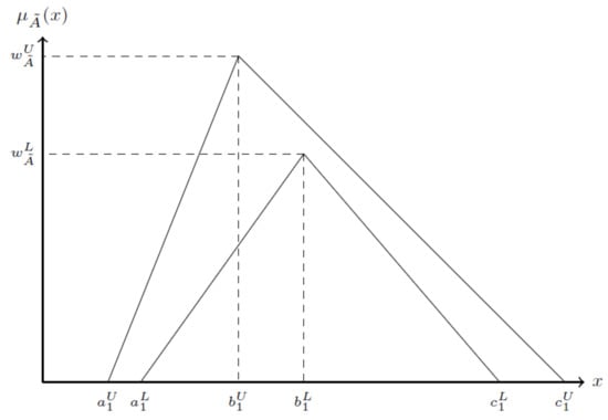
Figure 1.
Interval-valued triangular fuzzy numbers example (symmetrical and asymmetrical case).
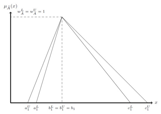
Figure 2.
Normalized interval-valued triangular fuzzy numbers example (asymmetrical case).
Definition 6.
Geometric mean
Let be n NIVTFNs. Then, the geometric mean of can be defined as
3. COMET Method with NIVTFNs
This section is devoted to a theoretical description of the proposed approach to solving MCDM problems with the use of NIVTFNs and COMET. The whole procedure has been divided into five colliding steps described below. Let be a set of alternatives and be the set of criteria. The whole decision-making process by using the COMET method and NIVTFNs is presented in Figure 3.
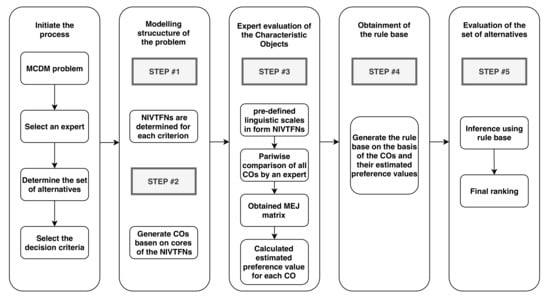
Figure 3.
The flowchart with proposed approach by using NIVFNs and the COMET method.
Step 1: Define the space of the problem
Let be the family of all NIVTFNs and be a collection of some NIVTFNs which are selected for each criterion . As a result, the following families of NIVTFNs can be obtained for each criterion as follows:
Now, we need to find the core of each NIVTFNs selected for each criterion . Afterwards, the core of each criterion is obtained which can be described as the core of each NIVTFN involved in the families as mentioned above, i.e.,
Step 2: Generate the COs
The all possible COs can be obtained by taking the Cartesian product of all as follow:
As the result of this, the following ordered sets are obtained containing all the cores of respective NIVTFNs as:
where is the count of all the COs.
Step 3: Rank and evaluate the COs
Collect the opinion of expert on the importance of all the COs via pairwise comparisons as represented by square matrix called the matrix of expert judgment (. The experts are requested to provide their assessments about by using the pre-defined linguistic scales in the form of NIVTFNs which can express the relative importance of one CO over another. The can expressed as
Each is NIVTFN which denotes the degree to which is preferred to .
Step 4: Preference values of COs
In this step, we will find two vectors known as and P. The vector called the vector of summed judgments is found by calculating the geometric mean of the corresponding elements in the form of NIVTFNs from the . This is represented by where each is NIVTFN and is obtained by taking the geometric mean of as discussed in Equation (1). The next vector which actually contains the preference values of all the COs can be computed by the following formula
Step 5: Inference in a fuzzy model and final ranking
As every alternative can be represented with a set of crisp numbers such as
where the following conditions must be satisfied for each element of .
To get the final ranking of the alternatives corresponding to each criterion for each , we proceed as follows:
The activated rules (COs) i.e., the group of those COs where the membership function of each alternative is non-zero are
The number of COs are obviously where Let be the approximate values of preference of the activated rules (COs) which were already calculated in Step 4. We denote the value of each family of NIVTFNs at where and . It should be noted that each member of this family is an interval of the form where for each and .
By using Definition 1, the preference value of each alternative in the form of interval can be computed as sum of the product of the preference values of all the COs and the fulfillment degrees of corresponding elements of , i.e.,
The final preference value of each alternative can be found by calculating the mean value of the corresponding preference interval i.e.,
Finally, the final ranking of alternatives is obtained by sorting the final preference values of alternatives. The greater the preference value, the better the alternative .
4. An Illustrative Example
In this section, we solve an illustrative example by using proposed approach. This example and presented calculations are intended to help the reader to understand the presented method. It will allow using the given technique to various types of problems by readers with a lower level of expertise in fuzzy sets and their extensions.
Let us consider the problem of selecting the new tank to buy by the government for the army. A tank is used as a primary armored fighting vehicle for front-line combat. The basic parameters providing good combat value and maneuverability are firepower, strong armor, good quality tracks, and a powerful engine. Let us say that we should analyze ten offers (alternatives). Each one was assessed separately in the three criteria, according to Firepower (FP), Battlefield Maneuverability (BM), and Engine Power (EP). The offers performance is presented in the form of a decision matrix with established three criteria and reference ranking by using expert knowledge, which can be seen in Table 1. The detailed calculation procedure will be presented in the next 5 steps.

Table 1.
The performance matrix and reference ranking of the alternatives.
Step 1: Suppose that and represent the three families of subsets of selected for the criteria , and respectively, where
The graphical representations of the families and for each criterion , and can be seen in Figure 4, Figure 5 and Figure 6 respectively. The cores for each family with respect to each criterion is determined as and .
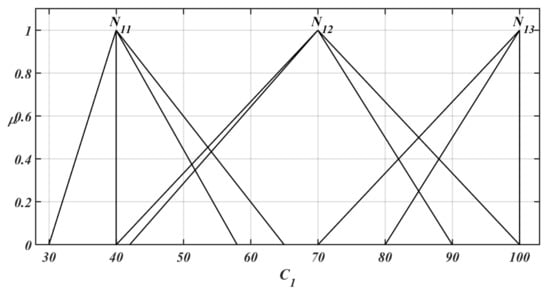
Figure 4.
Graphical representation of NIVTFNs for .
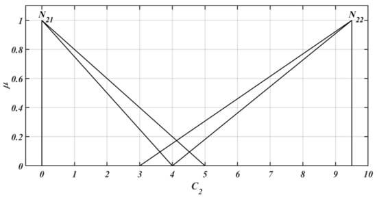
Figure 5.
Graphical representation of NIVTFNs for .
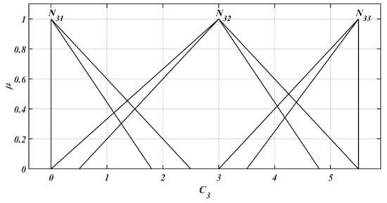
Figure 6.
Graphical representation of NIVTFNs for .
Step 2: The solution of COMET is obtained for different numbers of COs which can be obtained by taking the Cartesian product of the sets and . The list of all the COs with their set values are given as under:
Step 3: For the comparison of COs, suppose that the expert provides his/her pairwise judgments in the form of pre-defined linguistic scales in the form of NIVTFNs as expressed in Table 2. The most preferred CO will get linguistic variable “absolutely important”, the largest weaker CO will get linguistic variable “weakly important” and the COs with same comparison will get the linguistic variable “equally important”.

Table 2.
Pre-defined linguistic scales in the form of NIVTFNs.

Table 3.
Matrix of Expert Judgments part (1/2).

Table 4.
Matrix of Expert Judgments part (2/2).
Step 4: Now, we calculate the vector based on as mentioned in Step 4. The first component can be computed by using Equation (1) as follows:
On similar lines, the remaining components of the vector are obtained as follows:
By using Equation (2), the preference values of all the COs are then computed as
where are obtained in the following by using Equation (3).
Step 5: The preference interval indicating the approximate preference value of the first alternative is computed by using Formula (6), which is given as follows:
The final preference value of can be found by calculating the mean score value as
Similarly, the final preference values of all the remaining alternatives are obtained which are presented in Table 5.

Table 5.
Ranking of Alternatives with COMET using NIVTFNs (Rank), TOPSIS (), and reference ranking (), where relative closeness.
However, to compare result of our proposed method, TOPSIS method is applied to solve the same problem. The positive ideal solution and negative ideal solution are determined, and the relative closeness coefficients and final ranking are presented in Table 5.
The final ranking obtained by TOPSIS method is and the most desirable alternative is . However, by using the COMET method with NIVTFNs, the ranking of the alternatives is which adequately match as those with the ranking obtained in the TOPSIS method as well as the reference ranking .
In the proposed approach, the ranking has been determined as an average of the received intervals. The best and the worst alternatives have the same place in the ranking, and correlation is very high (). However, some important differences are also observed in the ranking order, i.e., the alternatives , , and . The proposed approach takes into account the new type of uncertainty compared to the previous extension of COMET. The result obtained here is the interval number, the so-called preference interval. Based on uncertain data, it is not possible to obtain a certain solution. Let us look at the assessment of alternatives and (Figure 7). The new quality of our solution is justified and possible discrepancies. The interval measure for is greater, but only in 74.07% of the cases for random values from these orders, we will obtain such a dependence. The solutions obtained by TOPSIS are the certain numbers and the any difference in the ranking has not explanation. The example above shows how a complete decision-making process can be carried out in order to make the result more knowledgeable about alternatives than other methods. This approach ensures that the phenomenon of rank reversal is avoided.

Figure 7.
Graphical representation of the assessment of alternatives and .
5. Conclusions
The uncertainty and diversity of assessment information provided by the DMs can be well reflected and modeled using NIVTFNs. The NIVTFNs are very useful to express vagueness and uncertainty more accurately as compared to fuzzy sets. Therefore, we synthesis a new method based on the COMET method and NIVTFNs. In that way, we obtained a helpful technique for solving MCDM problems under uncertain environment. In this study, we observed the difference between the proposed approach and TOPSIS methods for decision-making under uncertainty. We show that using preference intervals is more accurate and can justify the difference between rankings in an uncertain environment. Results of this approach are still free of rank reversal paradox due to the application of COMET, and it also permits decision-making under uncertain environment, especially where imprecise pieces of evidence and information are main hurdles for the decision-maker.
The presented approach is also following actual research trends in terms of methodological backgrounds. This paper provides theoretical manipulations of the extended approach of MCDM. It establishes a degree of membership in the form of interval instead of a crisp number, which is more suitable to tackle uncertainty during decision-making processes. To illustrate the whole calculation procedure of the COMET method using NIVTFNs, we studied a simple example. Future work will be geared towards the formulation of a comprehensive COMET-based system to support decision-making with an awareness of practical relevance and utility. Moreover, further research direction on the use of this approach and how to compare different rankings in the uncertain environment. As the next future works, we research the COMET method and:
- interval-valued intuitionistic fuzzy sets,
- hesitant fuzzy linguistic term sets,
- hesitant intuitionistic fuzzy linguistic term sets,
- etc.
Author Contributions
Conceptualization: S.F., W.S., S.U., T.R., J.W.; Formal analysis: S.F., W.S., S.U., T.R., J.W.; Investigation: S.F., W.S., S.U., T.R., J.W.; Methodology: S.F., W.S., S.U., T.R., J.W.; Validation: S.F., W.S., S.U., T.R., J.W.; Visualization: S.F., W.S., S.U., T.R., J.W.; Writing—original draft: S.F., W.S., S.U., T.R., J.W.; Writing—review editing: S.F., W.S., S.U., T.R., J.W. All authors have read and agreed to the published version of the manuscript.
Funding
The work was supported by the National Science Centre, Decision No. DEC-2016/23/N/HS4/01931, and by the Faculty of Computer Science and Information Technology, West Pomeranian University of Technology, Szczecin statutory funds.
Acknowledgments
The authors would like to thank the editor and the anonymous reviewers, whose insightful comments and constructive suggestions helped us to significantly improve the quality of this paper.
Conflicts of Interest
The authors declare no conflict of interest.
References
- Zadeh, L.A. Fuzzy Sets. Inf. Control 1965, 8, 338–353. [Google Scholar] [CrossRef]
- Bellman, R.E.; Zadeh, L.A. Decision-Making in a Fuzzy Environment. Manag. Sci. 1970, 17, B-141–B-273. [Google Scholar] [CrossRef]
- Masumpoor, S.; Yaghobi, H.; Ahmadieh Khanesar, M. Adaptive sliding-mode type-2 neuro-fuzzy control of an induction motor. Expert Syst. Appl. Int. J. 2015, 42, 6635–6647. [Google Scholar] [CrossRef]
- Jankowski, J.; Kazienko, P.; Wątróbski, J.; Lewandowska, A.; Ziemba, P.; Zioło, M. Fuzzy multi-objective modeling of effectiveness and user experience in online advertising. Expert Syst. Appl. 2016, 65, 315–331. [Google Scholar] [CrossRef]
- Chang, W.J.; Kuo, C.P.; Ku, C.C. Intelligent fuzzy control with imperfect premise matching concept for complex nonlinear multiplicative noised systems. Neurocomputing 2015, 154, 276–283. [Google Scholar] [CrossRef]
- Jankowski, J.; Lewandowska, A.; Watróbski, J.; Ziemba, P.; Salabun, W. Modeling the Perceptual Response from Effects Oriented Web Components Towards Lower Intrusiveness. In Proceedings of the 20th International Conference on Knowledge Based and Intelligent Information and Engineering Systems, KES2016, York, UK, 5–7 September 2016; pp. 147–158. [Google Scholar]
- Al-Obeidat, F.; Al-Taani, A.T.; Belacel, N.; Feltrin, L.; Banerjee, N. A fuzzy decision tree for processing satellite images and landsat data. Procedia Comput. Sci. 2015, 52, 1192–1197. [Google Scholar] [CrossRef]
- Piegat, A.; Sałabun, W. Comparative analysis of MCDM methods for assessing the severity of chronic liver disease. In International Conference on Artificial Intelligence and Soft Computing; Springer: Cham, Switzerland, 2015; pp. 1–14. [Google Scholar]
- Deveci, M.; Demirel, N.Ç.; John, R.; Özcan, E. Fuzzy multi-criteria decision making for carbon dioxide geological storage in Turkey. J. Nat. Gas Sci. Eng. 2015, 27, 692–705. [Google Scholar] [CrossRef]
- Amin, F.; Fahmi, A.; Abdullah, S.; Ali, A.; Ahmad, R.; Ghani, F. Triangular cubic linguistic hesitant fuzzy aggregation operators and their application in group decision making. J. Intell. Fuzzy Syst. 2018, 34, 1–15. [Google Scholar] [CrossRef]
- Tseng, M.-L.; Lim, M.; Wu, K.-J.; Zhou, L.; Bui, D.T.D. A novel approach for enhancing green supply chain management using converged interval-valued triangular fuzzy numbers-grey relation analysis. Resour. Conserv. Recycl. 2018, 128, 122–133. [Google Scholar] [CrossRef]
- Tseng, M.L. Implementation and performance evaluation using the fuzzy network balanced scorecard. Comput. Educ. 2010, 55, 188–201. [Google Scholar] [CrossRef]
- Yu, D. Triangular Hesitant Fuzzy Set and Its Application to Teaching Quality Evaluation. J. Inf. Comput. Sci. 2013, 10, 1925–1934. [Google Scholar] [CrossRef]
- Faizi, S.; Rashid, T.; Sałabun, W.; Zafar, S.; Wątróbski, J. Decision making with uncertainty using hesitant fuzzy sets. Int. J. Fuzzy Syst. 2018, 20, 93–103. [Google Scholar] [CrossRef]
- Montes, R.; Sanchez, A.M.; Villar, P.; Herrera, F. Teranga Go!: Carpooling Collaborative Consumption Community with multi-criteria hesitant fuzzy linguistic term set opinions to build confidence and trust. Appl. Soft Comput. 2018, 67, 941–952. [Google Scholar] [CrossRef]
- Rodríguez, R.M.; Martínez, L.; Torra, V.; Xu, Z.S.; Herrera, F. Hesitant Fuzzy Sets: State of the Art and Future Directions. Int. J. Intell. Syst. 2014, 29, 495–524. [Google Scholar] [CrossRef]
- Torra, V. Hesitant Fuzzy Sets. Int. J. Intell. Syst. 2010, 25, 529–539. [Google Scholar] [CrossRef]
- Rashid, T.; Husnine, S.M. Multicriteria group decision making by using trapezoidal valued hesitant fuzzy sets. Sci. World J. 2014, 2014, 304834. [Google Scholar] [CrossRef]
- Ngan, S.C. A unified representation of intuitionistic fuzzy sets, hesitant fuzzy sets and generalized hesitant fuzzy sets based on their u-maps. Expert Syst. Appl. 2017, 69, 257–276. [Google Scholar] [CrossRef]
- Qian, G.; Wang, H.; Feng, X. Generalized hesitant fuzzy sets and their application in decision support system. Knowl. -Based Syst. 2013, 37, 357–365. [Google Scholar] [CrossRef]
- Atanassov, K.; Gargov, G. Interval valued intutionistic fuzzy sets. Fuzzy Sets Syst. 1989, 31, 343–349. [Google Scholar] [CrossRef]
- Deveci, M.; Öner, S.C.; Canıtez, F.; Öner, M. Evaluation of service quality in public bus transportation using interval-valued intuitionistic fuzzy QFD methodology. Res. Transp. Bus. Manag. 2019, 2019, 100387. [Google Scholar] [CrossRef]
- Zhou, H.; Wang, J.; Li, X.; Wang, J.Q. Intuitionistic hesitant linguistic sets and their application in multi-criteria decision making problems. Int. J. Oper. Res. 2016, 16, 131–160. [Google Scholar] [CrossRef]
- Karczmarczyk, A.; Jankowski, J.; Sałabun, W. Linguistic Query Based Quality Evaluation of Selected Image Search Engines. Procedia Comput. Sci. 2017, 112, 1809–1818. [Google Scholar] [CrossRef]
- Wang, J.Q.; Wu, J.T.; Wang, J.; Zhang, H.Y.; Chen, X.H. Interval-valued hesitant fuzzy linguistic sets and their applications in multi-criteria decision-making problems. Inf. Sci. 2014, 288, 55–72. [Google Scholar] [CrossRef]
- Zadeh, L.A. The concept of a linguistic variable and its application to approximate reasoning-I. Inf. Sci. 1975, 8, 199–249. [Google Scholar] [CrossRef]
- Shih, H.S.; Shyur, H.J.; Lee, E.S. An extension of TOPSIS for group decision making. Math. Comput. Model. 2007, 45, 801–813. [Google Scholar] [CrossRef]
- Yoon, K.P.; Kim, W.K. The behavioral TOPSIS. Expert Syst. Appl. 2017, 89, 266–272. [Google Scholar] [CrossRef]
- Ziemba, P.; Wątróbski, J.; Zioło, M.; Karczmarczyk, A. Using the PROSA method in offshore wind farm location problems. Energies 2017, 10, 1755. [Google Scholar] [CrossRef]
- Ayhan, M.B. A Fuzzy AHP Approach for Supplier Selection Problem: A Case Study in a Gearmotor Company. arXiv 2013, arXiv:1311.2886. [Google Scholar] [CrossRef]
- Bayazit, O. Use of AHP in decision-making for flexible manufacturing systems. J. Manuf. Technol. Manag. 2005, 16, 808–819. [Google Scholar] [CrossRef]
- Gholipour, R.; Jandaghi, G.; Rajaei, R. Contractor selection in MCDM context using fuzzy AHP. Iran. J. Manag. Stud. 2014, 7, 151–173. [Google Scholar]
- Sałabun, W.; Ziemba, P.; Wątróbski, J. The rank reversals paradox in management decisions: The comparison of the AHP and COMET methods. Smart Innov. Syst. Technol. 2016, 56, 181–191. [Google Scholar]
- Bayazit, O. Use of analytic network process in vendor selection decisions. Benchmarking Int. J. 2006, 13, 566–579. [Google Scholar] [CrossRef]
- Bayazit, O.; Karpak, B. An analytical network process-based framework for successful total quality management (TQM): An assessment of Turkish manufacturing industry readiness. Int. J. Prod. Econ. 2007, 105, 79–96. [Google Scholar] [CrossRef]
- Büyüközkan, G.; Güleryüz, S.; Karpak, B. A new combined IF-DEMATEL and IF-ANP approach for CRM partner Evaluation. Int. J. Prod. Econ. 2017, 191, 194–206. [Google Scholar] [CrossRef]
- Piegat, A.; Sałabun, W. Identification of a Multicriteria Decision—Making Model Using the Characteristic Objects Method. Appl. Comput. Intell. Soft Comput. 2014, 2014, 536492. [Google Scholar] [CrossRef]
- Sałabun, W. The Characteristic Objects Method: A new distance based approach to multi-criteria decision-making problems. J. Multi Criteria Decis. Anal. 2015, 22, 37–50. [Google Scholar] [CrossRef]
- Sałabun, W. The Characteristic Objects Method: A new approach to Identify a multi-criteria group decision-making problems. Int. J. Comput. Appl. Technol. 2014, 5, 1597–1602. [Google Scholar]
- Sałabun, W.; Karczmarczyk, A.; Wątróbski, J.; Jankowski, J. Handling Data Uncertainty in Decision Making with COMET. In Proceedings of the 2018 IEEE Symposium Series on Computational Intelligence (SSCI), Bangalore, India, 18–21 November 2018; pp. 1478–1484. [Google Scholar]
- Sałabun, W.; Karczmarczyk, A.; Wątróbski, J. Decision-Making using the Hesitant Fuzzy Sets COMET Method: An Empirical Study of the Electric City Buses Selection. In Proceedings of the 2018 IEEE Symposium Series on Computational Intelligence (SSCI), Bangalore, India, 18–21 November 2018; pp. 1485–1492. [Google Scholar]
- Wang, J.Q.; Wang, J.; Chen, Q.H.; Zhang, H.Y.; Chen, X.H. An outranking approach for multi-criteria decision-making with hesitant fuzzy linguistic term sets. Inf. Sci. 2014, 280, 338–351. [Google Scholar] [CrossRef]
- Figueira, J.R.; Mousseau, V.; Roy, B. ELECTRE methods. Int. Ser. Oper. Res. Manag. Sci. 2016, 233, 155–185. [Google Scholar]
- Mousavi, M.; Gitinavard, H.; Mousavi, S.M. A soft computing based-modified ELECTRE model for renewable energy policy selection with unknown information. Renew. Sustain. Energy Rev. 2017, 68, 774–787. [Google Scholar] [CrossRef]
- Brans, J.P.; Mareschal, B.; Vincke, P. PROMETHEE: A New Family of Outranking Methods in Multicriteria Analysis. Oper. Res. 1984, 3, 477–490. [Google Scholar]
- Brans, J.P.; de Smet, Y. PROMETHEE methods. In Multiple Criteria Decision Analysis; Springer: New York, NY, USA, 2016; pp. 187–219. [Google Scholar]
- Wu, Y.; Wang, Y.; Chen, K.; Xu, C.; Li, L. Social sustainability assessment of small hydropower with hesitant PROMETHEE method. Sustain. Cities Soc. 2017, 35, 522–537. [Google Scholar] [CrossRef]
- Ziemba, P. NEAT F-PROMETHEE—A new fuzzy multiple criteria decision making method based on the adjustment of mapping trapezoidal fuzzy numbers. Expert Syst. Appl. 2018, 110, 363–380. [Google Scholar] [CrossRef]
- Soares De Mello, J.C.C.B.; Fernandes, J.E.M.; Gomes, L.F.A.M. Multicriteria selection of an aircraft with NAIADE. In Proceedings of the 1st International Conference on Operations Research and Enterprise Systems (ICORES-2012), Vilamoura, Portugal, 2–6 February 2012; pp. 427–431. [Google Scholar]
- Pastijn, H.; Leysen, J. Constructing an outranking relation with ORESTE. Int. Ser. Mod. Appl. Math. Comput. Sci. 1989, 1255–1268. [Google Scholar] [CrossRef]
- Guitouni, A.; Martel, J.-M.; Bélanger, M.; Hunter, C. Multiple criteria courses of action selection. Mil. Oper. Res. 2008, 13, 35–50. [Google Scholar] [CrossRef]
- Wątróbski, J.; Jankowski, J.; Ziemba, P.; Karczmarczyk, A.; Zioło, M. Generalised framework for multi-criteria method selection. Omega 2019, 86, 107–124. [Google Scholar] [CrossRef]
- Farhadinia, B. Distance and similarity measures for higher order hesitant fuzzy sets. Knowl. Based Syst. 2014, 55, 43–48. [Google Scholar] [CrossRef]
- Wang, J.; Wang, J.-Q.; Zhang, H.-Y.; Chen, X.-H. Distance-Based Multi-Criteria Group Decision-Making Approaches with Multi-Hesitant Fuzzy Linguistic Information. Int. J. Inf. Technol. Decis. Mak. 2017, 16, 1069–1099. [Google Scholar] [CrossRef]
- Van der Helm, P.A. Weber-Fechner behavior in symmetry perception? Atten. Percept. Psychophys. 2010, 72, 1854–1864. [Google Scholar] [CrossRef]
- Gitinavard, H.; Mousavi, S.M.; Vahdani, B. Soft computing-based new interval-valued hesitant fuzzy multi-criteria group assessment method with last aggregation to industrial decision problems. Soft Comput. 2017, 21, 3247–3265. [Google Scholar] [CrossRef]
- Gorzalczany, M.B. A method of inference in approximate reasoning based on interval-valued fuzzy sets. Fuzzy Sets Syst. 1987, 21, 1–17. [Google Scholar] [CrossRef]
- Lee, C.-S.; Chung, C.-C.; Lee, H.-S.; Gan, G.-Y.; Chou, M.-T. An interval-valued fuzzy number approach for supplier selection. J. Mar. Sci. Technol. 2016, 24, 384–389. [Google Scholar]
- Yao, J.S.; Lin, F.T. Constructing a fuzzy flow-shop sequencing model based on statistical data. Int. J. Approx. Reason. 2002, 29, 215–234. [Google Scholar] [CrossRef]
- Dubois, D.; Prade, H. Operations on fuzzy Numbers. Int. J. Syst. Sci. 1978, 9, 613–626. [Google Scholar] [CrossRef]
- Piegat, A.; Landowski, M. Is an interval the right result of arithmetic operations on intervals? Int. J. Appl. Math. Comput. Sci. 2017, 27, 575–590. [Google Scholar] [CrossRef]
© 2020 by the authors. Licensee MDPI, Basel, Switzerland. This article is an open access article distributed under the terms and conditions of the Creative Commons Attribution (CC BY) license (http://creativecommons.org/licenses/by/4.0/).