On the Urban Link Fundamental Diagram Based on Velocity-Weighted Flow and Queue Length

Abstract

For uninterrupted traffic flow, it is well-known that the fundamental diagram (FD) describes the relationship between traffic flow and density under steady state. To study the characteristics of interrupted traffic flow on a signalized link, a link fundamental diagram (LFD) for urban roads is proposed in this paper. First, a new variable, which synthesizes traffic flow with the speed of each vehicle, is defined. Then, the link fundamental diagram is obtained by drawing a scatter-plot of the velocity-weighted flow versus queue length, which takes on a unimodal curve with an approximately symmetric shape. Finally, simulation studies are conducted by modeling an urban link based on the traffic simulation software VISSIM. Compared with the traditional fundamental diagram, the proposed link fundamental diagram is more intuitive for showing the relationship between traffic condition and queue length. The impacts of the cycle time, green time, and split on the proposed link fundamental diagram are studied. Simulation results show that the shape of the link fundamental diagram fundamentally is determined by the split. The critical point is correlated to split values, and the green time exerts a great influence on both the velocity-weighted flow and the critical queue length. The cycle time has little effect on the critical queue length but has a great influence on the velocity-weighted flow.

1. Introduction

Fundamental diagrams (FDs) show the speed-density or flow–density relationship, which has been considered as the foundation of traffic flow theory. The FD was first observed by Greenshields and derived a parabolic equation to describe the flow–density curve [1], and many studies on speed and density have been proposed based on the empirical data for freeways [2,3]. Edie points out that traffic behavior appears to be different at high and low concentrations and proposes a discontinuous exponential form [3]. The discontinuity between uncongested and congested flow regions of the FD is described by using an extensive data set collected on the Queen Elizabeth Way in Ontario [4]. For the phenomenon that high density and low average velocity of cars can spontaneously appear in a region, its nonlinear theory is presented in an initially homogeneous traffic flow [5]. Hypotheses and some results of the three-phase traffic theory are compared with the results of the fundamental diagram [6]. By defining the equilibrium in a new manner, a mixed-integer programming approach is proposed for piecewise constructing linear FD [7]. A family of speed–density models with a variable number of arguments are presented in [8]. Numerical and empirical results of the field theory are provided and the benchmarking was conducted for some traffic flow models [9]. The single-regime model was developed with a novel calibration approach using as few, albeit useful, parameters as possible [10]. A non-equilibrium traffic model considering the vehicle velocity was presented, which is hyperbolic and has two characteristic fields, and it is shown to exhibit correct queue-end behavior and can explain some of the observed traffic phenomena that challenge old models [11] To date, FDs have been used for traffic state evaluation, ramp control, variable speed limit control, highway capacity analysis, and level of service [12].

However, most of these studies on FDs have focused on uninterrupted traffic flows (e.g., freeway traffic flow), there is limited related research on interrupted traffic flows (e.g., an isolated signalized intersection, a signalized coordinated link, a network with signalized intersections). A two-step approach was proposed to deal with the flow–density relationship calibration for an urban environment rather than freeways, which required a series of data processing steps that include the data aggregation, data selection, and the calibration of flow–density relationships [13]. A simulation study was conducted to investigate the problem of interrupted traffic flow, which examined the relationship between traffic flow and density on a ring road [14]. An arterial fundamental diagram, describing the relationship between traffic flow and occupancy, was researched based on traffic data from a major artery [15,16,17]. The difficulty of studying the FD for interrupted traffic flows is that the relationship between traffic flow and density is significantly affected by signal operations [15], which leads to the complexity of the interrupted flow and frequent uneven fluctuations [16].

Daganzo, together with Geroliminis, provided empirical evidence for the existence of an urban-scale macroscopic fundamental diagram (MFD) for a network with many intersections by using field data and simulation data [18,19,20]. It was observed that, when the highly scattered plots of flow vs. density from individual fixed detectors were aggregated, the phenomenon of high divergence is nearly disappeared and points are concentrated along a well-defined curve [21]. However, the MFD and its analyses were applicable only when the number of links was large [15], and MFD is not well-defined for heterogeneous networks and often appears with a high scatter and hysteresis phenomena [22,23,24,25,26,27].

MFD reveals spatio-temporal patterns of macro-mobility; however, it is not enough for promoting local mobility. Micro-mobility also has its positive impacts, thus an explicit understanding of the spatio-temporal usage patterns is an urgent need for making urban planning and policies or laws to promote sustainable development of the micro-mobility [28]. Many studies have conducted on the large georeferenced data-sets for individuals mobility, studying the statistical laws at the base of human movements [29,30,31] and the dynamic properties of human mobility in urban environment [32,33]. Some statistical and dynamic properties of pedestrian mobility in Venice are studied in [34]. These research activities can provide new knowledge tools for improving the sustainability of the mobility demand in future cities under the framework of Complex Systems Physics.

Original studies usually described either the flow–density relationship or the velocity–density relationship, in other words, most of these approaches focus on using data from this point of view. However, the links and intersections of the urban road networks achieve mutual coordination [35], and also have frequent queuing and stopping phenomenon which was usually modeled separately. Therefore, it is necessary to explore methodologies describing traffic characters by synthesizing multiple data sources [36,37,38], rather than simply using the original flow–density relationship. Since the queuing phenomenon is more common in the urban links and the queue length can be easily detected by cameras, the density can be replaced with the queue length. By considering the differences in uninterrupted and interrupted traffic flows, the spatio-temporal patterns of macro-mobility are investigated based on queue data and integrated data.

The primary contribution of this study can be summarized as follows:

(a)

A variable named the velocity-weighted flow combining the flow and space-mean velocity of each vehicle is proposed, which contains characteristics of both velocities and flows.

(b)

A new kind of link fundamental diagram (LFD) based on the velocity-weighted flow and queue length is presented in this paper, which can show the relationship between traffic condition and queue length.

(c)

Features of the proposed LFD related to cycle times, green times, and splits are presented: The LFD shape is generally determined by the splits. Both the critical queue length and critical velocity-weighted flow increase with increasing green time. The critical queue length is more closely related to the green time than the cycle time.

The rest of the paper is structured as follows: a brief description of the test platform and the problem formulation are presented in Section 2. Section 3 provides a detailed description of the velocity-weighted flow and the LFD based on the velocity-weighted flow and queue length. Features of the LFD is presented in Section 4. Conclusions and suggestions for future work are presented in Section 5.

2. Problem Formulation

2.1. Traffic Flow Description

Before describing the model, some mathematical symbols are introduced in Table 1, and the piecewise functions are used to describe the model in different situations. The queue length is defined as the distance between the stop line of a link and the position of the last vehicle in a queue. The traditional flow q (veh/h) is the number of vehicles passing through a point or section of a road in a unit [39]; the commonly used formula is

$$\begin{array}{c}\hfill q=\frac{N}{\Delta t}\end{array}$$

(1)

where N is the number of vehicles passing through a point or section of a road during $\Delta t$.

Table 1. List of Symbols.

Symbol	Explanation
$v_i\left(t\right)$	the velocity of vehicle i at time step t
$V_{free}$	free-flow velocity
$V_f$	following velocity
$x_i\left(t\right)$	distance from vehicle i to stop line at time step t
$l\left(t\right)$	queue length at time step t
$\alpha$	Discharge shock wave
$\beta$	queuing shock wave
$k_m$	density when following with vehicles
$k_j$	jam density
s	saturation flow
g	green time
r	red time
C	cycle time
$t_0$	beginning of the cycle
q	traffic flow
$q_C$	traffic flow passing an intersection in one cycle
$q_g$	arriving flow during green time
$\overline{q}$	velocity-weighted traffic flow

The relationship of flow and queue length in one cycle can be described with the following model:

$$\begin{array}{cc}\hfill & q_C=k_{j}l\left(t_0\right)+q_g,\mathrm{if}l\left(t_0\right)k_j<gs\hfill \\ \hfill & q_C=\frac{gs}{C},\mathrm{if}l\left(t_0\right)k_j>gs\hfill \end{array}$$

(2)

where $t_0$ is the beginning of the cycle, that is, traffic light turns green. The number of queuing vehicles $l\left(t_0\right)k_j$ is queue length $l\left(t_0\right)$ multiplied by the queue density (jam density) $k_j$, the number of discharged vehicles in one cycle is the green time g multiplied by saturated flow s. If $l\left(t_0\right)k_j<gs$, the existing queued vehicles will be discharged before the end of green time, and arriving flow $q_g$ will also flow toward the downstream. Assuming the distribution of $q_g$ is uniform, q will increase with the increasing $l\left(t_0\right)$ until link capacity is reached. If $l\left(t_0\right)k_j>gs$, the discharged vehicles are only $gs$ because when the queue is longer than a certain length, the link facilities can not serve so many vehicles, such that congestion. At the end of one cycle, $l\left(t_0\right)$ will update, and the flow will once again follow the law of Equation (2).

To validate this model, we utilize the micro traffic simulation software VISSIM to simulate an urban link to study the relationship of q and l. VISSIM is an advanced and flexible traffic simulation software. It can simulate complex vehicle interactions realistically on a microscopic level, and it can also model demand, supply, and behavior in detail. A 580-m long urban link is simulated in VISSIM, which is controlled by a traffic signal, as shown in Figure 1, and the background is Southern College Road, Haidian District, Beijing.

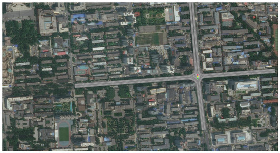
Figure 1. The diagram of a link in VISSIM.

The traffic data are produced under a random demand from no vehicles to the maximal flow. The flow can be directly measured according to the flow detector, and the queue length can be obtained by the queue detector in VISSIM. In fact, current transportation facilities at the intersection are also capable of measuring these data. The vehicle’s information can also be obtained, as shown in Table 2.

Table 2. Vehicle data information.

Symbol	Quantity	Sample
i	vehicle number	No. 549
$t_i$	moment of being positioned	600 (s)
$v_i$	instantaneous velocity	31.27 (km/h)
$d_i$	distance from vehicle to link entrance	386.48 (m)
$lin{k}_i$	The number of the link where the vehicle is located	No. 30
$L_i$	length of the link	826.41 (m)

When the signal cycle and the split are fixed, the relationship of queue length versus flow is as shown in Figure 2a. It can be observed that when the queue length l is less than 100 m, the flow q increases with increasing queue length. When the queue length l is greater than 100 m, q reaches the maximum value and remains unchanged. This phenomenon is caused by the limit of the link capacity: when the queue length is shorter than a certain value, the queue can be served and discharged with increasing flow. Once reaching the limit of link capacity, the traffic flow is the maximum that the link can provide.

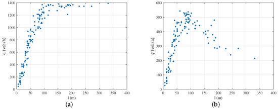
Figure 2. Comparison of the traditional FD and the proposed urban link FD: (a) scatter diagram of traditional flow and queue length; (b) scatter diagram of the velocity-weighted flow and queue length.

Because the traffic is supposed to be congested when the queue length is long, however, this phenomenon can’t be reflected from Figure 2a since its flow remains unchanged when the queue length is long. The FD with the shape of a single peak curve will more match people’s expectations and is conducive to the analysis of traffic congestion.

2.2. Vehicle Velocity Description

However, only the flow does not contain all traffic information, such as speed. When the queue length is short or even nonexistent, the driver simply needs to keep pace with the other vehicles; usually, without stopping, vehicles on an urban road can travel at a faster velocity, as shown in Figure 3 with the black line, and the average speed of the vehicle on the road is fast, but the flow is small. As the queue length increases, vehicles have to stop many times, as shown in Figure 3 with the blue line. The average speed of the vehicle is slowed down, but the flow is increasing until it doesn’t change if the downstream links have space.

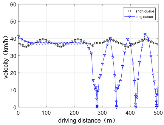
Figure 3. Vehicle speed versus driving distance for different queue length.

To describe these dynamics and better understand the usefulness of considering vehicle velocity, a model of velocity concerning queue length and time is established. To facilitate understanding and modeling, vehicle speed was divided into three categories, i.e., free flow velocity $V_{free}$, following velocity $V_f$ and stop velocity $V_s=0$, and the velocity of a vehicle in a link will be evolving with the queue length and time.

When a cycle time begins, which is defined as that traffic light turns green from red, there exist three conditions, that is, the vehicle isn’t queuing and is moving toward the end of the queue at free-flow velocity (Condition S1); the vehicle is queuing at a stop velocity (Condition S2); and the vehicle is following the vehicle in front at velocity $V_f$ (Condition S3). A vehicle may transform its state among S1, S2, and S3 when going through a link after many cycles.

Condition S1 means the vehicle i is running with free-flow speed at time step $t_0$, which is the green time beginning. Vehicle i will run with velocity $v_i$ from $t_0$ to $t_0+\frac{x_i\left(t_0\right)-l\left(t_0\right)}{V_{free}}$, as Formula (3) describes. Because the discharge shock wave $\alpha$ also begins propagating from the stop line to the end of queue, if the discharge shock wave arrive the end of queue late than the vehicle i, the vehicle will queue with speed $v_i=0$, as Formula (4) describes. Until the discharge shock wave arrives, then vehicle i will start and follow the vehicle in front with a relatively low speed $V_f$, as Formula (4a) describes. Note that this is under a precondition that the queue vehicles can not be discharged in one cycle (i.e., $l\left(t_0\right)k_j>gs$). When the green time finishes, there are $l\left(t_0\right)k_j-gs$ vehicles left and the length is $\frac{l\left(t_0\right)k_j-gs}{k_m}$, and the queue shock wave will begin, if the queue shock wave meets vehicle i (i.e., time $t_0+g+\frac{l\left(t_0\right)k_j-gs}{k_m\beta }$), vehicle i will stop and begin queue until the end of this cycle, as Formula (4b) describes. If the discharge shock wave arrives, and the end of queue is earlier than vehicle i, vehicle i will run longer until $t_0+\frac{x_i\left(t_0\right)-l\left(t_0\right)}{V_{free}-V_f}$, as Formula (5) describes. In addition, if vehicle i catches up with the front vehicle before the end of green time, it will run with speed $V_f$ until the end of green time, as Formula (5a) describes. If vehicle i exits the link during this time, its speed is $V_f$ all the time. If vehicle i doesn’t exit the link during this time, the vehicle will run with $V_f$ until the queue shock wave meets vehicle i, as Formula (5b) describes. Then, vehicle i will stop until the end of the cycle, as Formula (5c) describes.

Condition S1:

$$\begin{array}{cc}\hfill & v_i\left(t\right)=V_{free},t_0\le t<t_0+\frac{x_i\left(t_0\right)-l\left(t_0\right)}{V_{free}}\hfill \end{array}$$

(3)

$$\begin{array}{cc}\hfill & v_i\left(t\right)=0,t_0+\frac{x_i\left(t_0\right)-l\left(t_0\right)}{V_{free}}\le t<t_0+\frac{l\left(t_0\right)}{\alpha },\mathrm{if}\frac{l\left(t_0\right)}{\alpha }>\frac{x_i\left(t_0\right)-l\left(t_0\right)}{V_{free}}\hfill \end{array}$$

(4)

$$\begin{array}{cc}\hfill & v_i\left(t\right)=V_f,t_0+\frac{l\left(t_0\right)}{\alpha }\le t<t_0+g+\frac{l\left(t_0\right)k_j-gs}{k_m\beta },\mathrm{if}l\left(t_0\right)k_j-gs>0\hfill \end{array}$$

(4a)

$$\begin{array}{cc}\hfill & v_i\left(t\right)=0,t_0+g+\frac{l\left(t_0\right)k_j-gs}{k_m\beta }\le t<t_0+C\hfill \end{array}$$

(4b)

$$\begin{array}{cc}\hfill & v_i\left(t\right)=V_{free},t_0+\frac{x_i\left(t_0\right)-l\left(t_0\right)}{V_{free}}\le t<t_0+\frac{x_i\left(t_0\right)-l\left(t_0\right)}{V_{free}-V_f},\mathrm{if}\frac{l\left(t_0\right)}{\alpha }\le \frac{x_i\left(t_0\right)-l\left(t_0\right)}{V_{free}}\hfill \end{array}$$

(5)

$$\begin{array}{cc}\hfill & v_i\left(t\right)=V_f,t_0+\frac{x_i\left(t_0\right)-l\left(t_0\right)}{V_{free}-V_f}\le t<t_0+g,\mathrm{if}\frac{x_i\left(t_0\right)-l\left(t_0\right)}{V_{free}-V_f}<g\hfill \end{array}$$

(5a)

$$\begin{array}{cc}\hfill & v_i\left(t\right)=V_f,t_0+g\le t<t_0+g+\frac{l\left(t_0\right)k_j-gs}{k_m\beta },\mathrm{if}l\left(t_0\right)k_j-gs>0\hfill \end{array}$$

(5b)

$$\begin{array}{cc}\hfill & v_i\left(t\right)=0,t_0+g+\frac{l\left(t_0\right)k_j-gs}{k_m\beta }\le t<t_0+C\hfill \end{array}$$

(5c)

Condition S2 means that the vehicle i is queuing at time step $t_0$, which is the green time beginning, it needs to wait for the discharge shock wave and then run, as Formula (6) describes. If vehicle i begins to run, it will follow the front vehicle with a speed of $V_f$. However, there are also two situations: vehicle i will directly exit the link if $l\left(t_0\right)k_j<gs$ after $\frac{x_i\left(t_0\right)-l\left(t_0\right)}{V_{free}-V_f}$, as Formula (7) describes. If $l\left(t_0\right)k_j>gs$, vehicle i will meet the queue shock wave, as Formula (8) describes. However, if vehicle i does not meet the queue shock wave when the cycle time finishes, it will run with speed $V_f$ until the end of this cycle, as Formula (8a) describes, and the condition of vehicle i will turn to S2 for the next cycle. If vehicle i does not meet the queue shock wave when the cycle time finishes, it will run with speed 0 until the end of this cycle, as Formula (8b) describes.

Condition S2:

$$\begin{array}{cc}\hfill & v_i\left(t\right)=0,t_0\le t<t_0+\frac{l\left(t_0\right)}{\alpha }\hfill \end{array}$$

(6)

$$\begin{array}{cc}\hfill & v_i\left(t\right)=V_f,t_0+\frac{l\left(t_0\right)}{\alpha }\le t<t_0+\frac{l\left(t_0\right)}{\alpha }+\frac{l\left(t_0\right)}{V_f},\mathrm{if}l\left(t_0\right)k_j<gs\hfill \end{array}$$

(7)

$$\begin{array}{cc}\hfill & v_i\left(t\right)=V_f,t_0+\frac{l\left(t_0\right)}{\alpha }\le t<t_0+g+\frac{l\left(t_0\right)k_j-gs}{k_m\beta },\mathrm{if}l\left(t_0\right)k_j>gs\hfill \end{array}$$

(8)

$$\begin{array}{cc}\hfill & v_i\left(t\right)=V_f,t_0+g+\frac{l\left(t_0\right)k_j-gs}{k_m\beta }\le t<t_0+C\mathrm{if}r\le \frac{l\left(t_0\right)k_j-gs}{k_m\beta }\hfill \end{array}$$

(8a)

$$\begin{array}{cc}\hfill & v_i\left(t\right)=0,t_0+g+\frac{l\left(t_0\right)k_j-gs}{k_m\beta }\le t<t_0+C\mathrm{if}r>\frac{l\left(t_0\right)k_j-gs}{k_m\beta }\hfill \end{array}$$

(8b)

Condition S3 means that vehicle i is following the front vehicle at time step $t_0$, which is the green time beginning, it will meet the queue shock wave, as Formula (9) describes. There must be a queue $l\left(t_0\right)$ after the end of a cycle; otherwise, the situation is S1. If vehicle i meets the queue shock wave, its speed becomes zero and this remains for a while until the discharge shock wave passes through, as Formula (10) describes, where $x_i\left(t_0\right)-l\left(t_0\right))k_m/k_j+l\left(t_0\right)$ is the meeting place. If vehicle i meets the discharge shock wave before the end of green time, vehicle i will run with speed $V_f$ until meeting the queue shock wave, as Formula (10a,b) describe. Then, if the red time is enough, vehicle i will queue with 0 speed until the end of the cycle. However, if the red time $r<\frac{(x_i\left(t_0\right)-l\left(t_0\right))k_m+l\left(t_0\right)k_j-gs}{k_m\beta }$, vehicle i will exit the link with speed $V_f$. If vehicle i meets the discharge shock wave after the end of green time, the time meeting the queue shock wave is different with Formula (10a,b), but the basic principle is the same, so vehicle i will run with speed $V_f$, as Formula (11) describes; and then turns to zero until the end of cycle, as Formula (11a) describes.

Condition S3:

$$\begin{array}{cc}\hfill & v_i\left(t\right)=V_f,t_0\le t<t_0+\frac{x_i\left(t_0\right)-l\left(t_0\right)}{\beta }\hfill \end{array}$$

(9)

$$\begin{array}{cc}\hfill & v_i\left(t\right)=0,t_0+\frac{x_i\left(t_0\right)-l\left(t_0\right)}{\beta }\le t<t_0+\frac{(x_i\left(t_0\right)-l\left(t_0\right))k_m/k_j+l\left(t_0\right)}{\alpha }\hfill \end{array}$$

(10)

$$\begin{array}{cc}\hfill & v_i\left(t\right)=V_f,t_0+\frac{(x_i\left(t_0\right)-l\left(t_0\right))k_m/k_j+l\left(t_0\right)}{\alpha }\le t<t_0+g,\mathrm{if}g>\frac{(x_i\left(t_0\right)-l\left(t_0\right))k_m/k_j+l\left(t_0\right)}{\alpha }\hfill \end{array}$$

(10a)

$$\begin{array}{cc}\hfill & v_i\left(t\right)=V_f,t_0+g\le t<t_0+g+\frac{(x_i\left(t_0\right)-l\left(t_0\right))k_m+l\left(t_0\right)k_j-gs}{k_m\beta }\hfill \end{array}$$

(10b)

$$\begin{array}{cc}\hfill & v_i\left(t\right)=0,t_0+g+\frac{(x_i\left(t_0\right)-l\left(t_0\right))k_m+l\left(t_0\right)k_j-gs}{k_m\beta }\le t<t_0+C,\hfill \end{array}$$

(10c)

$$\begin{array}{c}\mathrm{if}r>\frac{(x_i\left(t_0\right)-l\left(t_0\right))k_m+l\left(t_0\right)k_j-gs}{k_m\beta }\hfill \end{array}$$

$$\begin{array}{cc}\hfill & v_i\left(t\right)=V_f,t_0+\frac{(x_i\left(t_0\right)-l\left(t_0\right))k_m/k_j+l\left(t_0\right)}{\alpha }\le t<t_0+2\frac{(x_i\left(t_0\right)-l\left(t_0\right))k_m/k_j+l\left(t_0\right)}{\alpha }-g\hfill \\ & +\frac{(x_i\left(t_0\right)-l\left(t_0\right))k_m+l\left(t_0\right)k_j-gs}{k_m\beta },\mathrm{if}g\le \frac{(x_i\left(t_0\right)-l\left(t_0\right))k_m/k_j+l\left(t_0\right)}{\alpha }\hfill \end{array}$$

(11)

$$\begin{array}{cc}\hfill & v_i\left(t\right)=0,t_0+2\frac{(x_i\left(t_0\right)-l\left(t_0\right))k_m/k_j+l\left(t_0\right)}{\alpha }-g+\frac{(x_i\left(t_0\right)-l\left(t_0\right))k_m+l\left(t_0\right)k_j-gs}{k_m\beta }\hfill \\ \hfill & \le t<t_0+C\hfill \end{array}$$

(11a)

In the next section, we will introduce a new definition including flow and velocity and link fundamental diagram, which will better fit people’s cognition of the traffic phenomenon.

3. Link Fundamental Diagram Based on Queue

3.1. The Definition of Velocity-Weighted Flow

A new definition called velocity-weighted flow, including flow and average velocity is given as follows:

$$\begin{array}{c}\hfill \overline{q}=\frac{{\displaystyle \sum _{i=1}^N}\frac{v_i}{V_{free}}}{\Delta t}\end{array}$$

(12)

where $\Delta t$ is a time interval passing through the link, N is the number of vehicles passing through the link during $\Delta t$, $v_i$ is the average velocity of vehicle i passing through the entire link, and $V_{free}$ is the free flow velocity. Formula (12) can be understood as a transformation of Formula (1), where the traditional traffic flow (1) is weighted by the average velocity of each vehicle in the flow. Thus, $\overline{q}$ includes both the information describing the number of vehicles passing through a link in a period and the information about the average speed of each vehicle passing through the link. To make sure that the dimension of $\overline{q}$ is still (veh/h), the velocity needs to be normalized in Formula (12), that is, $v_i/V_{free}$.

We can use the proposed queue-flow model and queue-velocity model to explain this appearance. The velocity of vehicles under condition S1 is likely to be $V_{free}$ when the queue length is short according to Formula (3) series. The velocity of vehicles under conditions S2 and S3 is likely to be $V_f$ when the queue length is short according to Formula (6) series, and they all have fewer stops.Because the flow q is low according to Formula (2), the weighted flow is correspondingly low. With the increasing queue, the flow is correspondingly increased, and the velocity of vehicles under condition S1, S2 and S3 is likely to be $V_f$ when the queue length is middling; moreover, the difference between $V_f$ and $V_{free}$ is not very great, so the weighted flow is correspondingly increased and maintain a large value. When the queue length is long, the vehicle velocity is low because some vehicles will stop and the vehicle even had to exit the link after several cycles, so the velocity-weighted flow is correspondingly decreased.

In summary, we can suggest that, when the link has few vehicles, the flow is small but the vehicle is fast, so $\overline{q}$ is not too small. Even if the traffic volume of a link reaches its maximum, but the vehicle is moving at a slower speed due to congestion, $\overline{q}$ is reduced until the link is completely blocked.

3.2. Drawing Link Fundamental Diagram

The scatter plot of traditional flow q versus queue length l is shown in Figure 2a, and the scatter plot of weighted flow $\overline{q}$ versus queue length l is shown in Figure 2b. Both of them are under the same simulation environment, but the proposed FD can present more dynamics of the traffic condition, which clearly demonstrates that traffic capacity will first increase and then decrease as queue lengths increase. The reasons are that: when the queue is short, less traffic flow means less $\overline{q}$; Traffic flow increases with the long queue, and the vehicle average velocity is relatively fast under this condition, so $\overline{q}$ is increasing. However, when the queue reaches a certain level, the long queue and increasing number of stops will lead to a decrease in the average speed of the vehicle, leading to a decrease in $\overline{q}$. Figure 2 shows that, when the queue length l is less than 100 m, $\overline{q}$ increases with the increase of l. When the queue length l is greater than 100 m, $\overline{q}$ decreases with an increase of l. This indicates that the average speed of vehicles passing through a link is significantly reduced when the queue length l is greater than 100 m, and it can be considered that the road traffic situation is congested. When the queue length l is approximately 100 m, which can be considered a critical queue length, both the traffic flow and the average speed of each car runs at a moderate speed.

In terms of traffic management, we assume the high traffic flow where the vehicles achieve a faster speed rate when passing through the link is more efficient. The definition of $\overline{q}$ considers both the number of vehicles passing in unit time and the average speed; moreover, the relationship of queue length versus $\overline{q}$ is an approximately symmetric curve which has an equilibrium point, so using this link fundamental diagram to distinguish the road traffic conditions will be clearer and more effective.

4. Characters of the Link Fundamental Diagram

4.1. Impact of Green Time on the Link Fundamental Diagram

The previous chapter outlines the proposed link fundamental diagram under the condition of a fixed signal cycle and green time. We now study additional characters of the link fundamental diagram with different signal cycles and green times.

In this chapter, we study $\overline{q}$ and l scatter plots under a fixed cycle but with different green times. Taking the period length of 60 s as an example, the scatter plots are shown in Figure 4a–e. The plot shows a single-peak curve, especially in Figure 4a–c. In Figure 4d,e, only the first half of the curve has high dispersion; since there is a long green time under this condition, the queue will be quickly dissipated, so the points in the second half are going to be sparse. According to Figure 4a–e, we can conclude that the green time can influence the shape of the link fundamental diagram. Summarizing the curves in Figure 4a–e, Figure 4f shows both the critical queue length and the velocity-weighted flow increase with the increasing of green time. These critical points are marked with a green hollow circle and are fitted as the dotted green line in Figure 4f, and the growth trend is also indicated by the green arrow line.

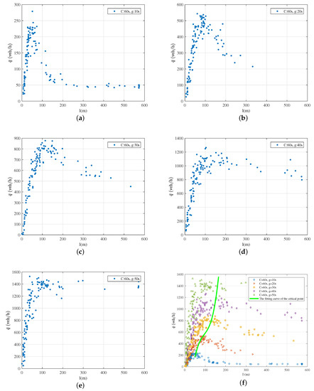
Figure 4. $\overline{q}$ versus queue length for different green times with a cycle time of 60 s: (a) cycle time C is 60 s, green time g is 10 s; (b) cycle time C is 60 s, green time g is 20 s; (c) cycle time C is 60 s, green time g is 30 s; (d) cycle time C is 60 s, green time g is 40 s; (e) cycle time C is 60 s, green time g is 30 s; (f) the summary figure and the fitting curve of the critical point.

To study the generality of this relationship, scatter plots of $\overline{q}$ and l under different green times of 60 s and 120 s are presented, as shown in Figure 5 and Figure 6, respectively. They also show the existence of the link fundamental diagram for other cycle times and green times, and both the critical queue length and the velocity-weighted flow increase with increasing green time.

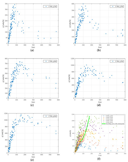
Figure 5. $\overline{q}$ versus queue length for different green times with a cycle time of 90 s: (a) cycle time C is 90 s, green time g is 20 s; (b) cycle time C is 90 s, green time g is 30 s; (c) cycle time C is 90 s, green time g is 40 s; (d) cycle time C is 90 s, green time g is 50 s; (e) cycle time C is 90 s, green time g is 60 s; (f) the summary figure and the fitting curve of the critical point.

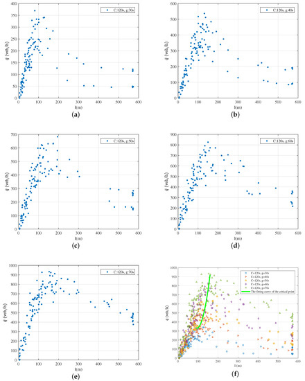
Figure 6. $\overline{q}$ versus queue length for different green time with a cycle time of 120 s: (a) cycle time C is 120 s, green time g is 30 s; (b) cycle time C is 120 s, green time g is 40 s; (c) cycle time C is 120 s, green time g is 50 s; (d) cycle time C is 120 s, green time g is 60 s; (e) cycle time C is 120 s, green time g is 70 s; (f) the summary figure and the fitting curve of the critical point.

We have studied the link fundamental diagram under a condition where the cycle time is fixed with different green times. Furthermore, we study the link fundamental diagram under the condition of a fixed green time with different cycle times. The critical points are marked with a green hollow circle for three signal cycles, and it can be seen that the critical weighted flow descends along the arrow from 530 to 220 for Figure 7a as well as Figure 7b,c, which means that the critical weighted flow varies greatly with the signal cycle. However, the critical queue length changes little with the signal cycle, which indicates that the critical queue length is more closely related to the green time than the cycle time, but the critical queue length changes little with the signal cycle.

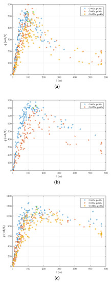
Figure 7. $\overline{q}$ versus queue length for different split: (a) split is 1/3; (b) split is 1/2; (c) split is 2/3.

4.2. The Impact of Split on the Link Fundamental Diagram

Figure 4, Figure 5 and Figure 6 have shown that green time can influence the critical weighted flow and the critical queue length, respectively. Figure 7 shows that cycle time can also influence the critical weighted flow and the critical queue length, but the critical queue length is relatively little affected by the cycle time. Because split is the ratio of effective green light time and cycle length for a phase, we will study the influence of split for the shape of the link fundamental diagram, critical weighted flow, and the critical queue length in this section.

The link fundamental diagram under different splits is shown in Figure 8. Figure 8a shows the weighted flow $\overline{q}$ versus length under the conditions where the split is $1/3$, that is, cycle time is 60 s with the green time of 20 s; the cycle time is 90 s with the green time of 30 s; the cycle time is 120 s with the green time of 40 s. Figure 8b,c shows the weighted flow $\overline{q}$ versus length under the conditions where the split is $1/2$ and $2/3$. It can be seen that the link fundamental diagram has a similar shape for the same split. We mark the critical weighted flow and the critical queue length with the green hollow circles, which indicates that the critical weighted flow and the critical queue length are very close for the same split. Therefore, we can conclude that the shape of the link fundamental diagram is usually determined by the split.

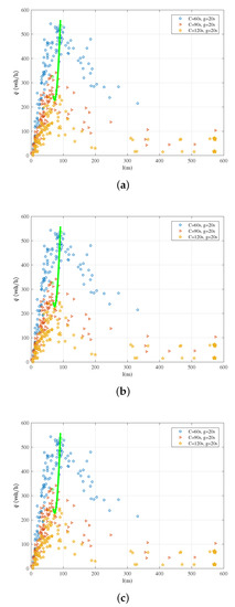
Figure 8. $\overline{q}$ versus queue length for different cycle times: (a) green time g is 20 s; (b) green time g is 30 s; (c) green time g is 40 s.

4.3. The Impact of Cycle Time on the Link Fundamental Diagram

To further study the impact of the split on the critical points, more experimental results are shown in Figure 9. The colored points represent the critical points (critical queue length, critical weighted flow), the number next to which represents the split value.

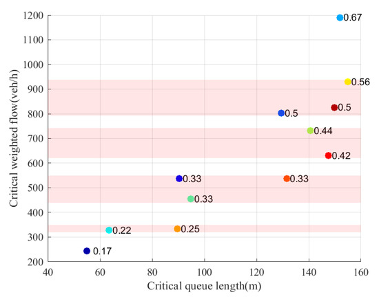
Figure 9. Scatter diagram of critical $\overline{q}$ vs. critical queue length for different splits.

The closed splits are highlighted on a light red background in Figure 9, and it can be seen that they have similar critical weighted flow. Moreover, the critical weighted flow increases with the increase of the split. Thus, we can conclude that the critical weighted flow is closely related to the split with a positive correlation.

5. Conclusions

A link fundamental diagram is presented in this paper according to queue length and the defined velocity-weighted flow. This study sets out to describe the properties of urban road traffic flow in a heuristic way. The results of this investigation show that the scatter plots take a relatively clear form of unimodal curves, that is, the velocity-weighted flow first increases and then decreases as the queue length increases, which means that the traffic ability increases first and then declines. Moreover, the characteristics of the link fundamental diagram are examined, including the impacts of green time, cycle time, and split. The correlation of critical weighted flow, critical queue length, green time, cycle time, and split are discussed. The new link fundamental diagram might help the traffic manager to evaluate the state of link congestion, or make appropriate control objectives, for example, keeping queue length below a certain value as a preventive means for avoiding congestion.

In the future, this study could be verified through field data and explained by a mathematical model, and the link fundamental diagram can also be used in traffic condition evaluations.

References

- Greenshields, B.D.; Bibbins, J.R.; Channing, W.S.; Miller, H.H. A study of traffic capacity. In Highway Research Board Proceedings; National Research Council (USA), Highway Research Board: Washington, DC, USA, 1935; Available online: https://www.semanticscholar.org/paper/A-study-of-traffic-capacity-Greenshields-Bibbins/a3f3c282a7a35b5265ee74757d0edfa163d69bad#citing-papers (accessed on 8 May 2020).
- Greenberg, H. An Analysis of Traffic Flow. Oper. Res. 1959, 7, 79–85. [Google Scholar] [CrossRef]
- Edie, L.C. Car-following and steady-state theory for noncongested traffic. Oper. Res. 1961, 9, 66–76. [Google Scholar] [CrossRef]
- Hall, F.L.; Allen, B.L.; Gunter, M.A. Empirical analysis of freeway flow–density relationships. Transp. Res. Part A Gen. 1986, 20, 197–210. [Google Scholar] [CrossRef]
- Kerner, B.S.; Konhäuser, P. Structure and parameters of clusters in traffic flow. Phys. Rev. E Statal Phys. Plasmas Fluids Relat. Interdiplinary Top. 1994, 50, 54. [Google Scholar] [CrossRef] [PubMed]
- Kerner, B.S. Three-Phase Traffic Theory and Highway Capacity. Phys. A Statal Mech. Appl. 2002, 333, 379–440. [Google Scholar] [CrossRef]
- Li, J.; Zhang, H.M. Fundamental Diagram of Traffic Flow: New Identification Scheme and Further Evidence from Empirical Data. Transp. Res. Rec. 2011, 2260, 50–59. [Google Scholar] [CrossRef]
- Wang, H.; Li, J.; Chen, Q.Y.; Ni, D. Logistic modeling of the equilibrium speed–density relationship. Transp. Res. Part A Policy Pract. 2011, 45, 554–566. [Google Scholar] [CrossRef]
- Ni, D.; Wang, H. A unified perspective on traffic flow theory. Part III: Validation and benchmarking. Appl. Math. Sci. 2013, 7, 1965–1982. [Google Scholar] [CrossRef][Green Version]
- Qu, X.; Wang, S.; Zhang, J. On the fundamental diagram for freeway traffic: A novel calibration approach for single-regime models. Transp. Res. Part B Methodol. 2015, 73, 91–102. [Google Scholar] [CrossRef]
- Zhang, H. A non-equilibrium traffic model devoid of gas-like behavior. Transp. Res. Part B Methodol. 2002, 36, 275–290. [Google Scholar] [CrossRef]
- Wang, D.; Ma, X.; Ma, D.; Jin, S. A Novel Speed–Density Relationship Model Based on the Energy Conservation Concept. IEEE Trans. Intell. Transp. Syst. 2017, 18, 1179–1189. [Google Scholar] [CrossRef]
- Leclercq, L. Calibration of Flow-Density Relationships on Urban Streets. Transp. Res. Rec. J. Transp. Res. Board 2005, 1934, 226–234. [Google Scholar] [CrossRef]
- Gartner, N.H.; Wagner, P. Traffic flow characteristics on signalized arterials. Transp. Res. Rec. J. Transp. Res. Board 2004, 1883, 94–100. [Google Scholar] [CrossRef]
- Wu, X.; Liu, H.X.; Geroliminis, N. An empirical analysis on the arterial fundamental diagram. Transp. Res. Part B Methodol. 2011, 45, 255–266. [Google Scholar] [CrossRef]
- Hallenbeck, M.E.; Ishimaru, J.M.; Davis, K.D.; Kang, J.M. Arterial performance monitoring using stop bar sensor data. In Proceedings of the 87th Annual Meeting of the Transportation Research Board, Washington, DC, USA, 13–17 January 2008. [Google Scholar]
- He, Z.; Ming, C.; Wang, L.; LI, M. Empirical Analysis of Urban Arterial Fundamental Diagram. In Proceedings of the 2018 37th Chinese Control Conference (CCC), Wuhan, China, 25–27 July 2018. [Google Scholar]
- Daganzo, C.F.; Geroliminis, N. An analytical approximation for the macroscopic fundamental diagram of urban traffic. Transp. Res. Part B Methodol. 2008, 42, 771–781. [Google Scholar] [CrossRef]
- Geroliminis, N.; Daganzo, C.F. Existence of urban-scale macroscopic fundamental diagrams: Some experimental findings. Transp. Res. Part B Methodol. 2008, 42, 759–770. [Google Scholar] [CrossRef]
- Ji, Y.; Daamen, W.; Hoogendoorn, S.; Hoogendoorn-Lanser, S.; Qian, X. Investigating the Shape of the Macroscopic Fundamental Diagram Using Simulation Data. Transp. Res. Rec. J. Transp. Res. Board 2010, 2161, 40–48. [Google Scholar] [CrossRef]
- Geroliminis, N.; Sun, J. Properties of a well-defined macroscopic fundamental diagram for urban traffic. Transp. Res. Part B Methodol. 2011, 45, 605–617. [Google Scholar] [CrossRef]
- Buisson, C.; Ladier, C. Exploring the Impact of Homogeneity of Traffic Measurements on the Existence of Macroscopic Fundamental Diagrams. Transp. Res. Rec. 2009, 2124, 127–136. [Google Scholar] [CrossRef]
- Mazloumian, A.; Geroliminis, N.; Helbing, D. The Spatial Variability of Vehicle Densities as Determinant of Urban Network Capacity. Philos. Trans. R. Soc. A Math. Phys. Eng. Sci. 2010, 368, 4627–4647. [Google Scholar] [CrossRef]
- Gayah, V.V.; Daganzo, C.F. Clockwise hysteresis loops in the Macroscopic Fundamental Diagram: An effect of network instability. Transp. Res. Part B Methodol. 2011, 45, 643–655. [Google Scholar] [CrossRef]
- Geroliminis, N.; Sun, J. Hysteresis phenomena of a Macroscopic Fundamental Diagram in freeway networks. Transp. Res. Part A Policy Pract. 2011, 45, 966–979. [Google Scholar] [CrossRef]
- He, Z.; He, S.; Guan, W. A figure-eight hysteresis pattern in macroscopic fundamental diagrams and its microscopic causes. Transp. Lett. 2014, 7, 133–142. [Google Scholar] [CrossRef]
- Xie, D.F.; Wang, D.Z.; Gao, Z.Y. Macroscopic analysis of the fundamental diagram with inhomogeneous network and instable traffic. Transp. A Transp. Sci. 2016, 12, 20–42. [Google Scholar] [CrossRef]
- Zhu, R.; Zhang, X.; Kondor, D.; Santi, P.; Ratti, C. Understanding spatio-temporal heterogeneity of bike-sharing and scooter-sharing mobility. Comput. Environ. Urban Syst. 2020, 81, 101483. [Google Scholar] [CrossRef]
- Brockmann, D.; Hufnagel, L.; Geisel, T. The scaling laws of human travel. Nature 2006, 439, 462–465. [Google Scholar] [CrossRef]
- Gonzalez, M.C.; Hidalgo, C.A.; Barabasi, A.L. Understanding individual human mobility patterns. Nature 2008, 453, 779–782. [Google Scholar] [CrossRef]
- Yan, X.Y.; Han, X.P.; Wang, B.H.; Zhou, T. Diversity of individual mobility patterns and emergence of aggregated scaling laws. Sci. Rep. 2013, 3, 2678. [Google Scholar] [CrossRef]
- Zhao, K.; Musolesi, M.; Hui, P.; Rao, W.; Tarkoma, S. Explaining the power-law distribution of human mobility through transportationmodality decomposition. Sci. Rep. 2015, 5, 1–7. [Google Scholar] [CrossRef]
- Gallotti, R.; Bazzani, A.; Rambaldi, S.; Barthelemy, M. A stochastic model of randomly accelerated walkers for human mobility. Nat. Commun. 2016, 7, 1–7. [Google Scholar] [CrossRef]
- Mizzi, C.; Fabbri, A.; Rambaldi, S.; Bertini, F.; Curti, N.; Sinigardi, S.; Luzi, R.; Venturi, G.; Davide, M.; Muratore, G.A. Unraveling pedestrian mobility on a road network using ICTs data during great tourist events. EPJ Data Sci. 2018, 7, 44. [Google Scholar] [CrossRef]
- Shen, Q.; Ban, X.; Guo, C. Urban Traffic Congestion Evaluation Based on Kernel the Semi-Supervised Extreme Learning Machine. Symmetry 2017, 9, 70. [Google Scholar] [CrossRef]
- Ning, Z.; Xia, F.; Ullah, N.; Kong, X.; Hu, X. Vehicular social networks: Enabling smart mobility. IEEE Commun. Mag. 2017, 55, 16–55. [Google Scholar] [CrossRef]
- Silva, T.H.; de Melo, P.O.V.; Almeida, J.M.; Viana, A.C.; Salles, J.; Loureiro, A.A. Participatory sensor networks as sensing layers. In Proceedings of the 2014 IEEE Fourth International Conference on Big Data and Cloud Computing, Sydney, NSW, Australia, 3–5 December 2014; pp. 386–393. [Google Scholar]
- Rodrigues, D.O.; Boukerche, A.; Silva, T.H.; Loureiro, A.A.F.; Villas, L.A. Combining taxi and social media data to explore urban mobility issues. Comput. Commun. 2018, 132, 111–125. [Google Scholar] [CrossRef]
- Lighthill, M.J.; Whitham, G.B. On kinetic waves, II. A theory of traffic flow on long crowded roads. Proc. R. Soc. A 1955, 229, 317–345. [Google Scholar]
Publisher’s Note: MDPI stays neutral with regard to jurisdictional claims in published maps and institutional affiliations. |
© 2020 by the authors. Licensee MDPI, Basel, Switzerland. This article is an open access article distributed under the terms and conditions of the Creative Commons Attribution (CC BY) license (http://creativecommons.org/licenses/by/4.0/).