Article

Reinforcement Learning Approach to Design Practical Adaptive Control for a Small-Scale Intelligent Vehicle

1
Key Laboratory of Advanced Manufacturing Technology for Automobile Parts, Ministry of Education, Chongqing University of Technology, Chongqing 400054, China
2
State Key Laboratory of Engines, Tianjin University, Tianjin 300072, China
*
Authors to whom correspondence should be addressed.
B.H. and J.L. equally contributed to this research work.
Symmetry 2019, 11(9), 1139; https://doi.org/10.3390/sym11091139
Submission received: 18 August 2019 / Revised: 3 September 2019 / Accepted: 4 September 2019 / Published: 7 September 2019

Abstract

:
Reinforcement learning (RL) based techniques have been employed for the tracking and adaptive cruise control of a small-scale vehicle with the aim to transfer the obtained knowledge to a full-scale intelligent vehicle in the near future. Unlike most other control techniques, the purpose of this study is to seek a practical method that enables the vehicle, in the real environment and in real time, to learn the control behavior on its own while adapting to the changing circumstances. In this context, it is necessary to design an algorithm that symmetrically considers both time efficiency and accuracy. Meanwhile, in order to realize adaptive cruise control specifically, a set of symmetrical control actions consisting of steering angle and vehicle speed needs to be optimized simultaneously. In this paper, firstly, the experimental setup of the small-scale intelligent vehicle is introduced. Subsequently, three model-free RL algorithm are conducted to develop and finally form the strategy to keep the vehicle within its lanes at constant and top velocity. Furthermore, a model-based RL strategy is compared that incorporates learning from real experience and planning from simulated experience. Finally, a Q-learning based adaptive cruise control strategy is intermixed to the existing tracking control architecture to allow the vehicle slow-down in the curve and accelerate on straightaways. The experimental results show that the Q-learning and Sarsa (λ) algorithms can achieve a better tracking behavior than the conventional Sarsa, and Q-learning outperform Sarsa (λ) in terms of computational complexity. The Dyna-Q method performs similarly with the Sarsa (λ) algorithms, but with a significant reduction of computational time. Compared with a fine-tuned proportion integration differentiation (PID) controller, the good-balanced Q-learning is seen to perform better and it can also be easily applied to control problems with over one control actions.

1. Introduction

Self-driving vehicles—which incorporate multiple complex systems to sense the surrounding environment, plan a path to a destination, and control steering and speed—have grown rapidly in the last few years [1,2]. There are hundreds of companies worldwide that are on track to have autonomous vehicle technology ready by 2020, including Toyota, Google, and Tesla [3]. Currently, one barrier to the academics and industry who wish to develop and test their intelligent control algorithm is the massive expense of the full-scale vehicles [4], not to mention the expense of constructing the test site in order to provide a safe, controlled environment for the testing of self-driving vehicles (for example, University of Michigan has spent $10 million developing an entire 32-acre mock city, Mcity, in order to serve as a providing ground for their intelligent vehicles [5]). One solution to this problem would be to develop a small-scale vehicle that could be used as a testing platform for intelligent vehicle technologies, without incurring the expense and safety hazards of a full-scale vehicle. Figure 1 shows the small- and full- scale vehicle platform for developing and testing the intelligent control algorithm for self-driving vehicles.
For the tracking and adaptive cruise control of an intelligent vehicle, the proportion integration differentiation (PID) control is a control loop mechanism employing feedback that is widely used in industrial control systems and a variety of other applications requiring continuously modulated control. It has been the classic type of controller since the mid-20th century and will continue as the most often used industrial control scheme, due to its remarkable effectiveness, simple implementation, and broad applicability [6,7]. However, the parameter setting processing of conventional PID controllers is very complicated and the results are hard to be satisfactory, which might cause a great waste of manpower, material resources, and equipment. There are some other PID variants, including expert PID control [8], fuzzy PID control [9], and neural network-based PID control [10], etc. Although they are said to perform better if tuned well, rich expert knowledge for the expert PID, sophisticated fuzzy control decision table for the fuzzy PID control, and fine-tuned neural network parameters for the neural network-based PID control are required, and this may prevent their widespread use for self-driving vehicles’ tracking and adaptive cruise control. Meanwhile, in the complex systems with high order, large lag, strong coupling, nonlinear and time-varying parameters, the traditional control theory which relies on mathematical models is still immature, and some methods are complicated and cannot be directly applied for industrial applications. In this context, it is urgent to construct a “model-free” intelligent algorithm to achieve end-to-end learning and intelligent control while taking the industrial need of simplicity and robustness into consideration.
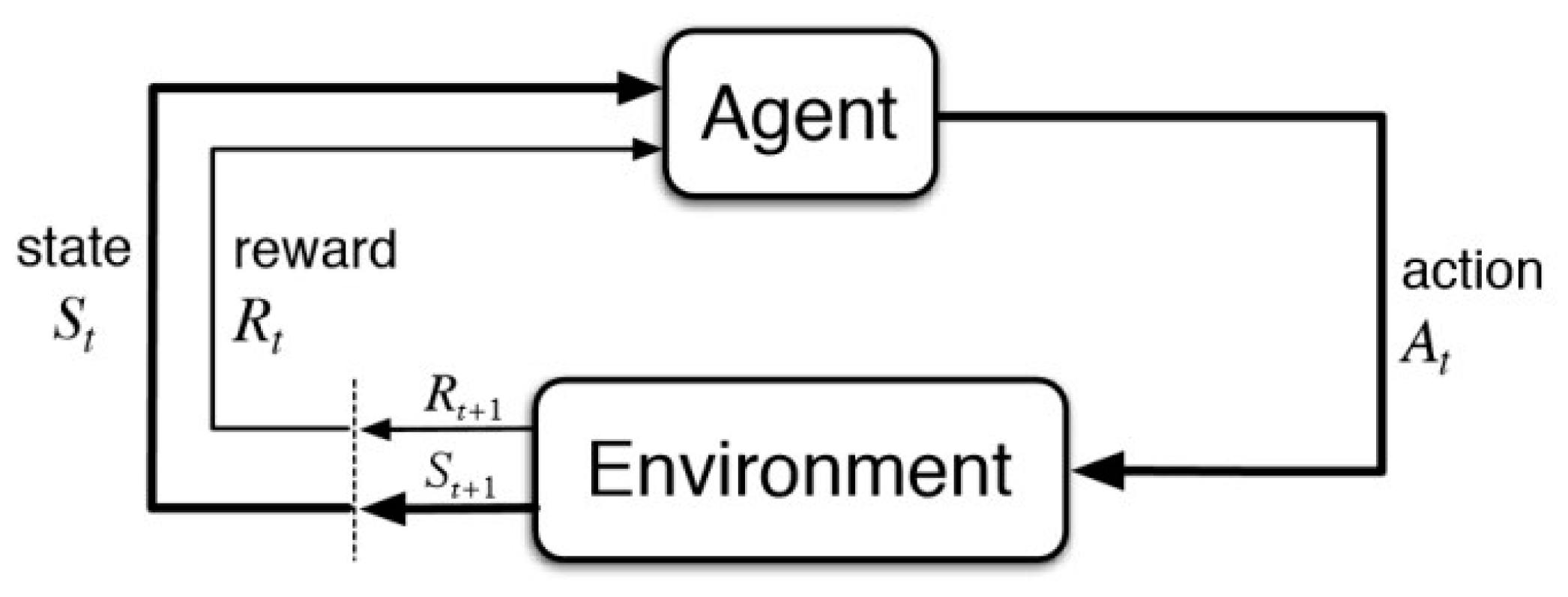
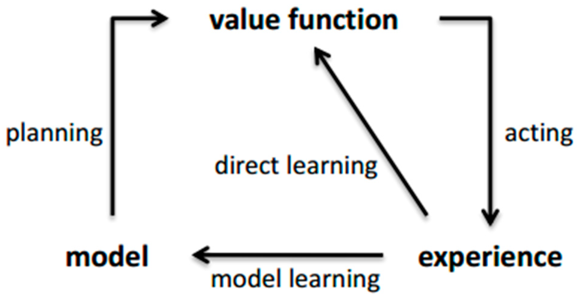
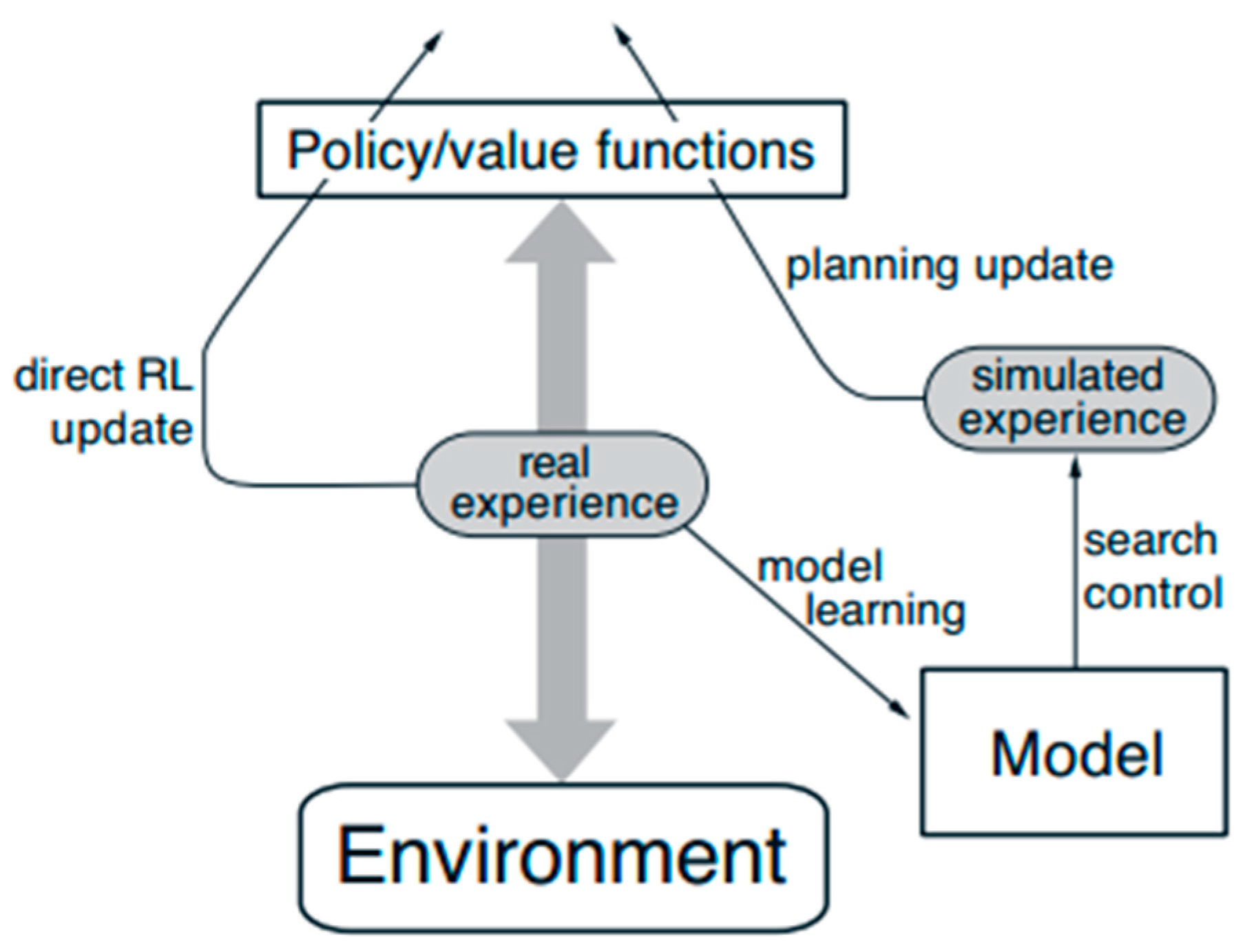
Reinforcement learning (RL), which is considered as one of three machine learning paradigms alongside supervised learning and unsupervised learning, is an area of machine learning concerned with how agents ought to take actions in an environment so as to maximize cumulative reward (see Figure 2). The theory of reinforcement learning, inspired by the psychology of behaviorism, focuses on online learning and tries to maintain a balance between exploration and exploitation. Different from supervised learning and unsupervised learning, reinforcement learning does not require any pre-given data, but obtains learning information and updates model parameters by receiving rewards (feedback) from the environment for actions. Due to its generality, it is studied in many other disciplines, such as game theory [11], control theory [12], operations research [13], information theory [14], simulation-based optimization [15], and multi-agent systems [16]. Temporal-difference (TD) learning, which is a combination of Monte Carlo ideas and dynamic programming (DP) ideas, is considered as one idea which is central and novel to reinforcement learning [17]. Like Monte Carlo methods, TD methods can learn directly from raw experience without a model of the environment’s dynamics. Like DP, TD methods update estimates based, in part, on other learned estimates, without waiting for a final outcome. In RL, there are two classes of TD methods: on-policy and off-policy. The most important on-policy algorithm includes Sarsa and Sarsa (λ), and one of the breakthroughs in off-policy reinforcement learning is known as Q-learning. Apart from the above pure model-free reinforcement learning method, some model-based methods can be intermixed to make the learning more efficient [18]. For example, Figure 3 shows the information flow in a Dyna-Q architecture. It includes planning, acting, model-learning, and direct RL—all occurring continuously. The planning method is the random-sample one-step tabular Q-planning method, and the direct RL method is one-step tabular Q-learning.
For the industrial application, the Q-learning algorithm was used to reduce the induction motor losses by controlling the magnetic currents in different torque loads, and approximately 50% power loss was reduced in comparison with the standard driver of motor when the motor works in low loads [19]. The Q-learning algorithm was also demonstrated to outperform the existing expert-based power management strategy on achieving better power performance trade-off, and it was more flexible in adapting to different workloads and hardware [20]. Anderlini et al. [21] presented the application of Q-learning algorithm for the optimal resistive control of a point absorber in order to maximize energy absorption in each sea state. They found that the algorithm can be converged towards the optimal controller damping in each sea state and this model-free approach ensures the algorithm adapts the changes to the device hydrodynamics over time and is unbiased by modelling errors. Sun et al. [22] proposed a hybrid module algorithm based on Q-learning to achieve the goal of maximizing the benefit to the network service provider. As for Sarsa, Aissani et al. [23] presented a multi-agent approach for the dynamic maintenance task scheduling for a petroleum industry production system. They showed that the agents can simultaneously ensure effective maintenance scheduling and continuous improvement of the solution quality by means of Sarsa algorithm. In addition, the Sarsa (λ) algorithm was proposed to select an optimal route in the stages of a supply chain that will balance the reverse condition of cost and time, and the experimental results show that Sarsa (λ) outperformed optimal route selection over the conventional Q-learning by exhibiting higher convergence speed, a lesser number of episodes to find optimal route, and a lesser computational time for different scenarios [24]. Li et al. [25] proposed a communication solution based on Dyna-Q algorithm to effectively avoid intelligent interference attacks, with better learning efficiency and faster convergence. Liu et al. [18] compared the Dyna-Q and Q-learning algorithms by applying them to the energy management strategy for a hybrid electric tracked vehicle. They indicated that although the Q-learning algorithm is faster than the Dyna-Q algorithm, its fuel consumption is 1.7% higher than that of the Dyna-Q algorithm. To the authors’ best knowledge, there are few literatures that systematically analyze the four mentioned RL techniques on sequential decision control problems for industrial products, and also for the self-driving vehicles’ tracking and adaptive cruise control, limited knowledge can be found to showcase the experimentally practical method to learn the optimal strategy from scratch based on the classical tabular RL methods.
Based on the above discussion, it is necessary to apply the RL techniques for the tracking and adaptive cruise control on a small-scale intelligent vehicle in order to a) systematically compare the different RL techniques under the experimental environment and b) provide references for the further development of RL techniques (including deep RL) on a full-scale intelligent vehicle. For the sake of achieving the tracking and longitudinal control performance, first the experimental setup of the small-scale intelligent vehicle is introduced. Subsequently, the model-free RL algorithm, including Q-learning, Sarsa, and Sarsa (λ), was conducted to develop and finally form the strategy to keep the vehicle within its lanes at constant and top longitudinal velocity. Furthermore, a model-based RL strategy (Dyna-Q) was built that incorporates learning from real experience and planning from simulated experience. Finally, in order to achieve the fastest lap time, a Q-learning based adaptive cruise control strategy was intermixed to the existing tracking control architecture to allow the vehicle to slow-down in the curve and accelerate on straightaways. The rest of this article is structured as follows: Section 2 describes the experimental setup for the small-scale intelligent vehicle. In Section 3, the RL based framework is proposed to realize the optimal tracking and adaptive cruise control. In Section 4, the corresponding experimental results will be illustrated to compare different RL techniques and a fine tuned PID algorithm. Section 5 concludes the article.

2. Experimental Setup

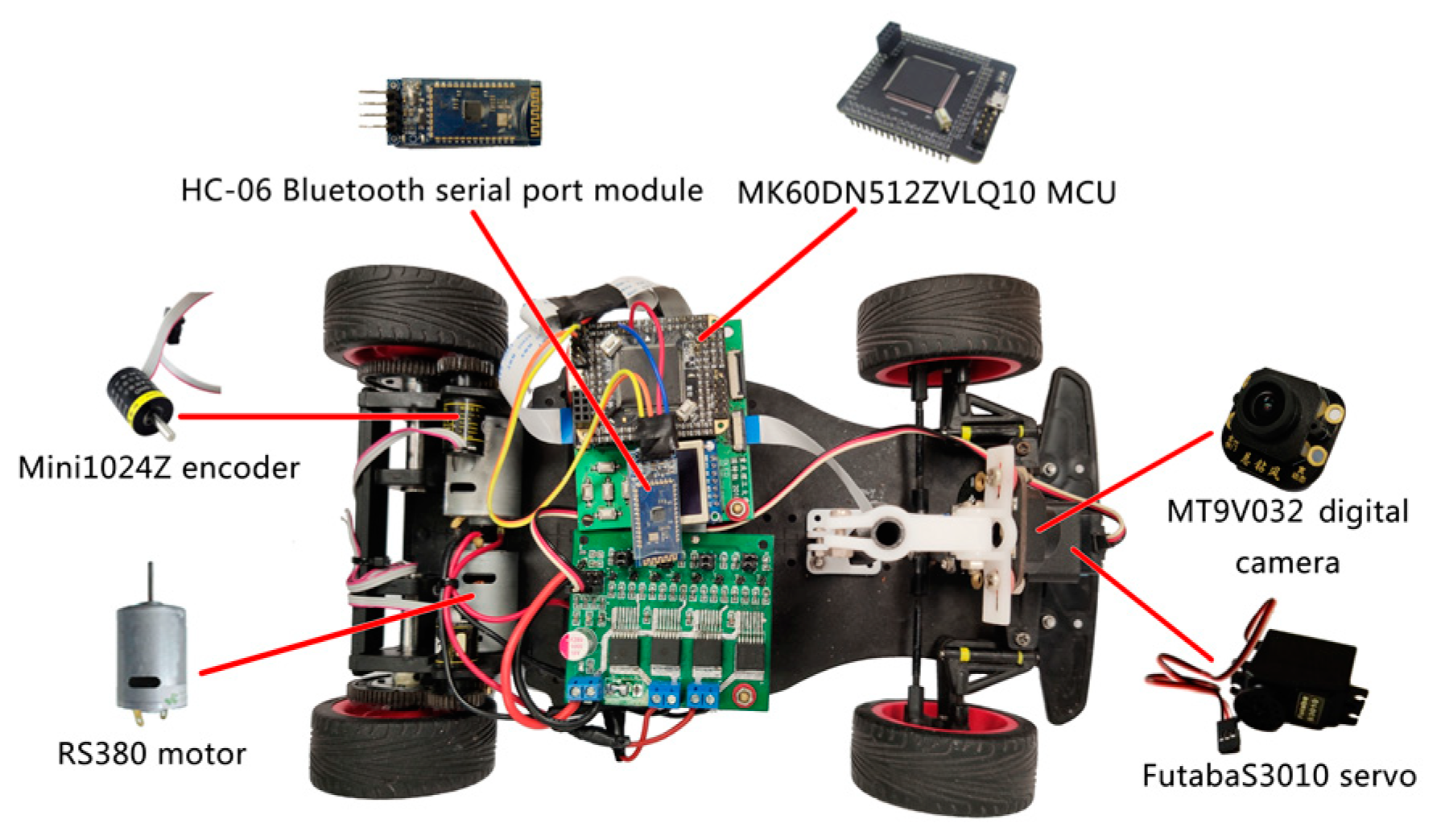
The experimental platform that the RL algorithm will be implemented on is shown in Figure 4. Like any other small-scale vehicle platform (such as the rapid autonomous complex-environment competing Ackermann-steering robots at Massachusetts Institute of Technology (MIT) [26] and the Berkeley autonomous race car at University of California, Berkeley [27]), this platform will help test various intelligent and adaptive control strategies on a physical vehicle system, thus providing references for the further development of full-scale intelligent vehicles. In order to focus on the RL techniques without spending too much time on the hardware debugging, we have designed the platform to use many purchased ordinary parts (in order to make it easy to transfer the knowledge acquired from this study to a full-scale intelligent vehicle) and to take advantage of low-cost manufacturing processes, such as 3D printing.
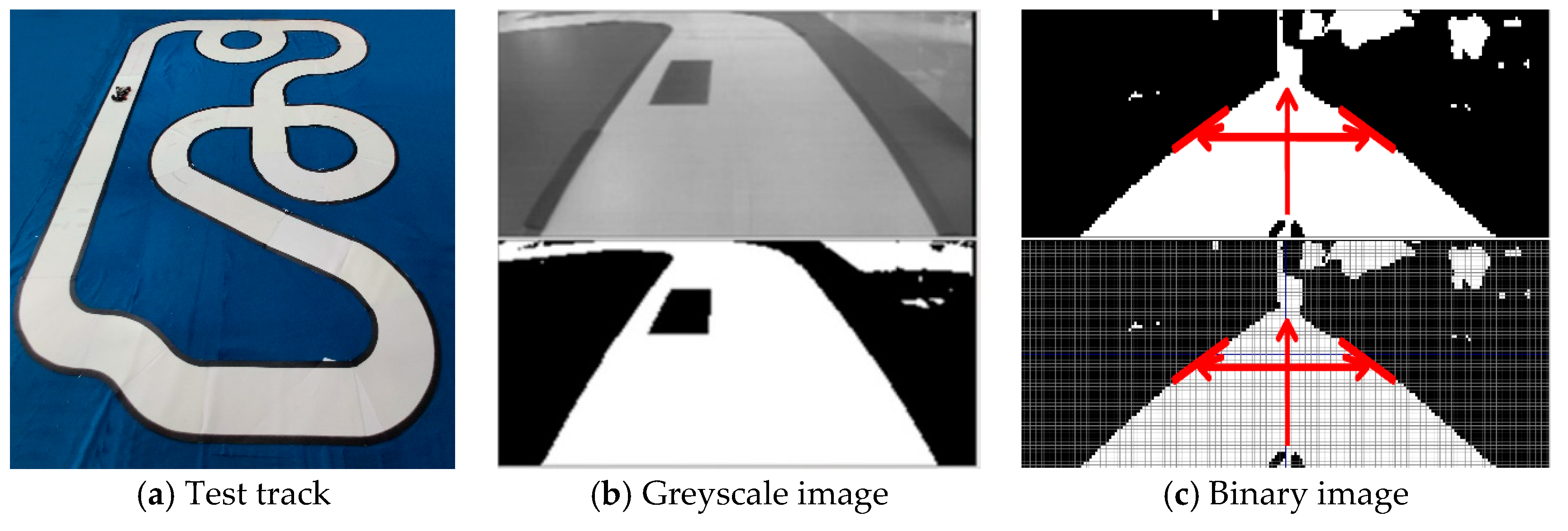
A MK60DN512ZVLQ10 Microprogrammed Control Unit (MCU) was used as the core control to obtain the experimental data from the sensor, and transmits the command to each actuator, in order to coordinate the operation as required. For actuators, a Futaba S3010 servo motor controls the steering of the vehicle body and an RS380 motor controls the speed of the vehicle. As for sensors, in this study, an MT9V032 digital camera was used to obtain the environment information (in this study, a simplified track is provided as shown in Figure 5a) which then can be converted to the offset from the track centerline. In detail, the camera first obtains the track image as shown in Figure 5b. Then, the gray image obtained by the digital camera is converted into a binarized map by software binarization to determine the road conditions in front of the vehicle (See Figure 5c). Finally, the distance between the black and white boundary at 23 cm in front of the vehicle body is found to determine the offset of the vehicle body from the centerline. Two 1024-line dual-phase incremental mini encoders were used to obtain the vehicle speed. By obtaining the encoder pulse for a period of time, the vehicle speed was calculated based on the wheel-to-encoder gear ratio and the wheel diameter. A HC-06 Bluetooth serial port module was used to achieve the interactive functions, so as to send the experimental data to the host computer.
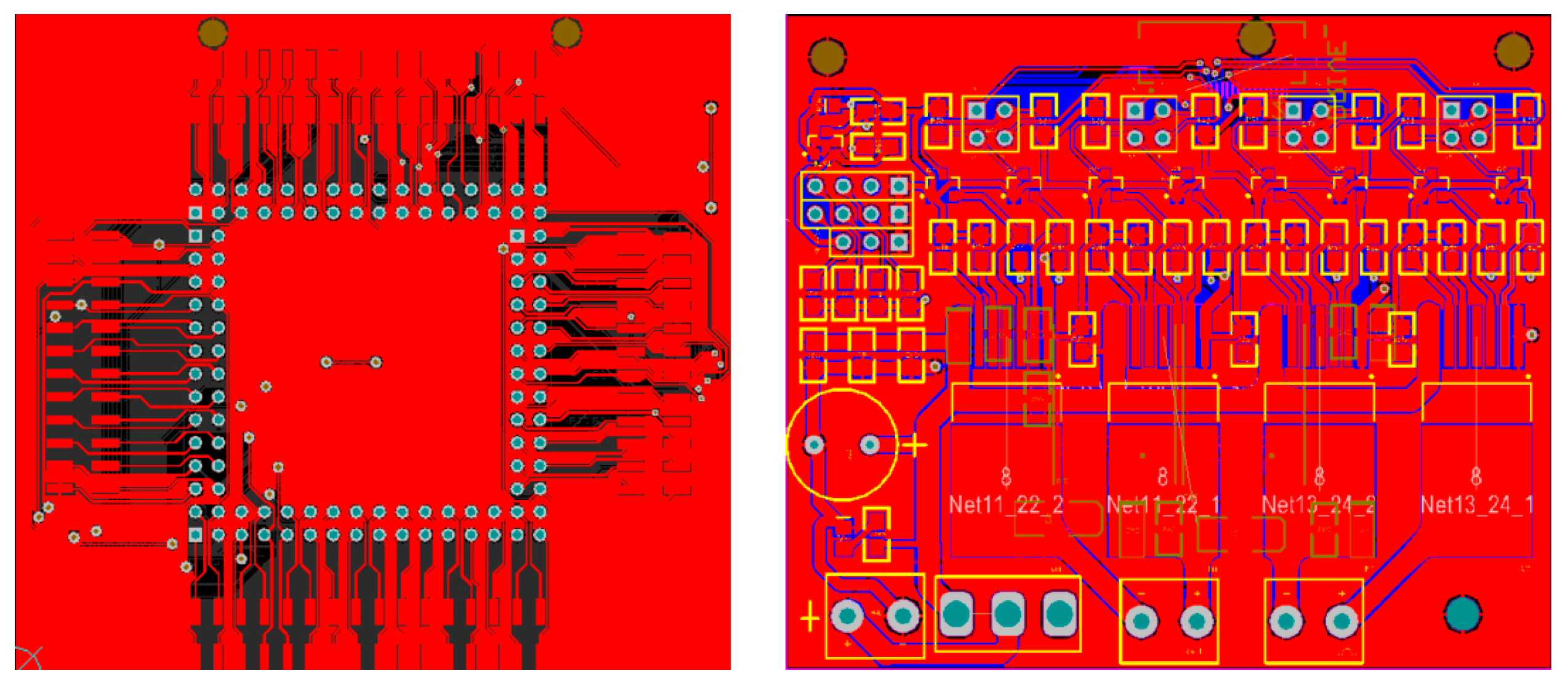
The small-scale intelligent vehicle is powered by a 7.2v, 2000 mAh nickel–cadmium battery. The hardware board, as shown in Figure 6, was used to connect the various functional components so that they can be controlled by the MCU to achieve the purpose of coordinated operation. It mainly includes the power supply circuit (power supply to MCU and to each module), each drive circuit involving identifying the control signal of the small current emitted by MCU, supplying sufficient energy to the steering servo motor and the speed motor to perform the corresponding actions, driving the camera to work according to the MCU instructions, and driving the wireless Bluetooth serial port module to transmit data functionally.

3. Control Strategy Based on Reinforcement Learning

3.1. Problem Formulation

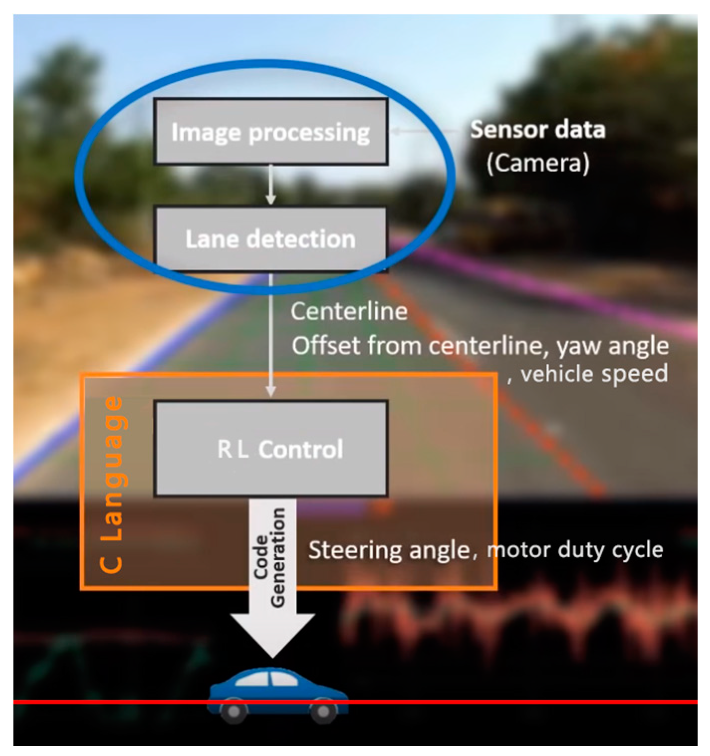
In this study, there are three control behaviors that need to be learned, namely, (a) tracking control at constant velocity, (b) tracking control at incrementally constant speed, and (c) tracking control at adaptive cruise velocity. In detail, the first task requires the small-scale vehicle to travel along the centerline of the test track while keeping the vehicle speed constant. The second task increases the control difficulty by making the vehicle learn the maximum speed that allows the vehicle to travel along the track centerline without running out of bounds. The ultimate aim of this study is to enable the vehicle to keep the vehicle along its centerline while learning to slow down or accelerate adaptively according to different road conditions. Unlike any other control techniques, the purpose of this study is to seek a practical method that enables the vehicle, in the real environment and in real time, to learn the control behavior on its own while adapting to the changing circumstances. Thus, it is necessary to design an algorithm that symmetrically considers both time efficiency and accuracy. Meanwhile, in order to realize adaptive cruise control specifically, a set of symmetrical control actions consisting of steering angle and vehicle speed needs to be optimized simultaneously. Figure 7 illustrates the control flow chart for the small-scale intelligent vehicle, in which the sensor data is used by the control unit to regulate the steering angle and motor duty cycle to keep the vehicle travelling along the centerline with required vehicle velocity.

3.2. The Key Concept of Reinforcement Learning

Reinforcement learning is the core technology of many artificial intelligence software. Compared to supervised learning and unsupervised learning in the machine learning field, RL uses a continuous “trial-and-error” mechanism and a “exploitation and exploration” balance without correct sample labeling [28]. Through the real-time perception of the feedback status of the environment (as a supervised signal of its actions), see Figure 2, the parameters are continuously adjusted to achieve the optimal sequential decision making for a given task. In the following, key concepts of the RL-based tracking and adaptive cruise control algorithm are formulated.
System state: In the RL algorithm, control action is directly determined by the system states. In this study, the offset from centerline, vehicle yaw angle, and vehicle velocity are selected to form a three-dimensional state space, i.e., s ( t ) = ( e ( t ) ,   φ ( t ) , v ( t ) ) T , where e ( t ) represents the offset from the centerline at time t, φ ( t ) , and v ( t ) represent yaw angle and vehicle speed at time t, respectively. Figure 8 illustrates the three defined states, in which the value after the servo represents a set of yaw angle states, the value after Pulse-Width Modulation (PWM) represents a set of vehicle speed states, and the number at the top of the figure represents a set of the offset from the centerline. It should be noted here that only a small number of states are chosen in this study in order to (a) facilitate the training process and (b) showcase the generalization ability of the RL techniques.
Control action: The decision-making on the steering servo motor which decides the vehicle steering angle and the motor which determines the vehicle speed are the core problem of the control strategy. We choose the steering angle of the servo motor and the duty cycle of the motor as the control actions, denoted as A ( t ) = ( μ ( t ) , ρ ( t ) ) , where t is the time step index. A ( t ) should be discretized in order to apply the RL-based algorithm, i.e., the entire action space is A = { A 1 , A 2 , A n } , where n is the degree of discretization and is the multiplication of the number of steering actions and the number of speed actions. In this study, for the first two tasks, we consider n as 9, and for the ultimate task, n is set to be 27 with three speed control actions added.
Immediate reward: Immediate reward is important in the RL algorithm because it directly influences the convergence curves and, in some cases, a fine adjustment of the immediate reward parameter can bring the final policy to the opposite poles [29]. The agent is always trying to maximize the reward, which it can obtain by taking the optimal action at each time step. Therefore, the immediate reward should be defined according to the optimization objective. The control objective of this work is to enable the vehicle to travel along the centerline (for task a, b, and c) and adaptively alter speed according to different road conditions (for task c). Keeping this objective in mind, the function of the offset from the centerline (for task a, b, and c) and the current vehicle speed are defined as the immediate reward. A large penalty value was introduced to penalize the situation when the vehicle is running out of the boundaries. In this experiment, when the vehicle is about to rush out of the runway at a long distance from the centerline, the vehicle is given a command to reverse the full steering angle and use this as the current action to update Q table in the current state. In the conventional process of RL, the experimental body has to be put back into the environment to continue learning when rushing out of boundaries, and this design can creatively make the experiment body correct itself and continue to learn when it is about to go out of bounds, which effectively reduces the human-made operational factors. Meanwhile, there is no need to supervise the learning process at all times, which greatly improves the learning efficiency. In the following, the equations for the immediate reward are given:
r ( t ) = e ( t ) 2 + ( 2 × v ( t ) ) 2 + 20
where r ( t ) is the immediate reward generated when the state change by taking an action at time t. As the objective is to maximize the cumulated rewards for a period of time, a negative sign is given before e ( t ) which is the offset from the centerline. v ( t ) represents the vehicles speed and a larger value of that without compromising the tracking performance should be given a larger reward.
Formally, the goal of this tracking and adaptive cruise control is to find the optimal control strategy, π * , that maps the observed states s t to the control action a t . Mathematically, the control strategy of this vehicle control can be formulated as an infinite horizon dynamic optimization problem, as follows:
R = t = 0 γ t r ( t )
where γ ( 0 , 1 ) is a discount factor that assures the infinite sum of cost function convergence. We used Q * ( s t , a t ) , i.e., the optimal value, to represent the maximum accumulative reward, which we can obtain by taking action a t in state s t , Q * ( s t , a t ) is calculated by the Bellman equation, whose equation is different for different RL techniques, as shown from Section 3.3 to Section 3.6.

3.3. The Q-Learning Algorithm

One of the early breakthroughs in RL was the development of an off-policy TD control algorithm known as Q-learning. The learning state-action function, Q, directly approximates q * , the optimal state-action function, independent of the policy being followed [30]. This dramatically simplifies the analysis of the algorithm and enables early convergence proofs. The pseudo-code of this algorithm can be seen in Algorithm 1, in which ϵ greedy means the control strategy is to behave greedily most of the time, but every once in a while, say with small probability, instead, select randomly from among all the actions with equal probability, independently of the state-action estimates.
Algorithm 1. The Q-learning algorithm pseudo code.
  Algorithm : RL : Q - learning   algorithm     1 . Initialize   Q ( s , a )   arbitrarily   2 . Repeat   ( for   each   episode ) :   3 .   Initialize   s   4 .   Repeat   ( for   each   step   of   episode ) :   5 .   Choose   a   from   s   using   policy   derived   from   Q ( e . g . ,   ε g r e e d y )   6 .   Take   action   a ,   observe   r , s   7 .   Q ( s , a ) Q ( s , a ) + α [ r + γ max a Q ( s , a ) Q ( s , a ) ]   8 .   s s   9 .   Until   s   is   terminal  

3.4. The Sarsa Algorithm

The full name of the Sarsa algorithm is state action reward state action (see Figure 9), which is also a kind of TD learning algorithm. It has a high degree of similarity with the Q-learning algorithm and it is also a value-based reinforcement learning algorithm that uses the Q function to find the optimal action selection strategy. Compared with the Q-learning algorithm, Sarsa has already chosen the next state and the next action at the current iteration, putting it into the on-policy algorithm category. This difference makes Sarsa more timid than Q-learning, because Q-learning always thinks about Q function maximization, thus making it greedy, regardless of other non-maxQ results. Compared with Q-learning, which can be described as greedy, bold, and brave, Sarsa is a conservative algorithm that is sensitive to control errors. Algorithm 2 shows the pseudo code for the Sarsa algorithm.
Algorithm 2. The Sarsa algorithm pseudo code.
  Algorithm : RL : Sarsa   algorithm     1 . Initialize   Q ( s , a )   arbitrarily   2 . Repeat   ( for   each   episode ) :   3 .   Initialize   s   4 .   Choose   a   from   s   using   policy   derived   from   Q ( e . g . ,   ε g r e e d y )   5 .   Repeat   ( for   each   step   of   episode ) :   6 .   Choose   a   from   s   using   policy   derived   from   Q ( e . g . ,   ε g r e e d y )   7 .   Take   action   a ,   observe   r , s   8 .   Q ( s , a ) Q ( s , a ) + α [ r + γ Q ( s , a ) Q ( s , a ) ]   9 .   s s ; a a ;   10 .   Until   s   is   terminal  

3.5. The Sarsa (λ) Algorithm

Sarsa (λ) is an upgraded version based on the Sarsa method. It can learn more efficiently on how to get the maximum accumulative reward. For Sarsa and Q-learning, both being one-step TD learning methods, they can only update the corresponding Q function (the step before getting the current reward) per time step, while Sarsa (λ) enables bootstrapping to occur over multiple steps, freeing us from the tyranny of the single time step [11]. This feature, in theory, is more capable of solving the control problem with sparse reward delays.
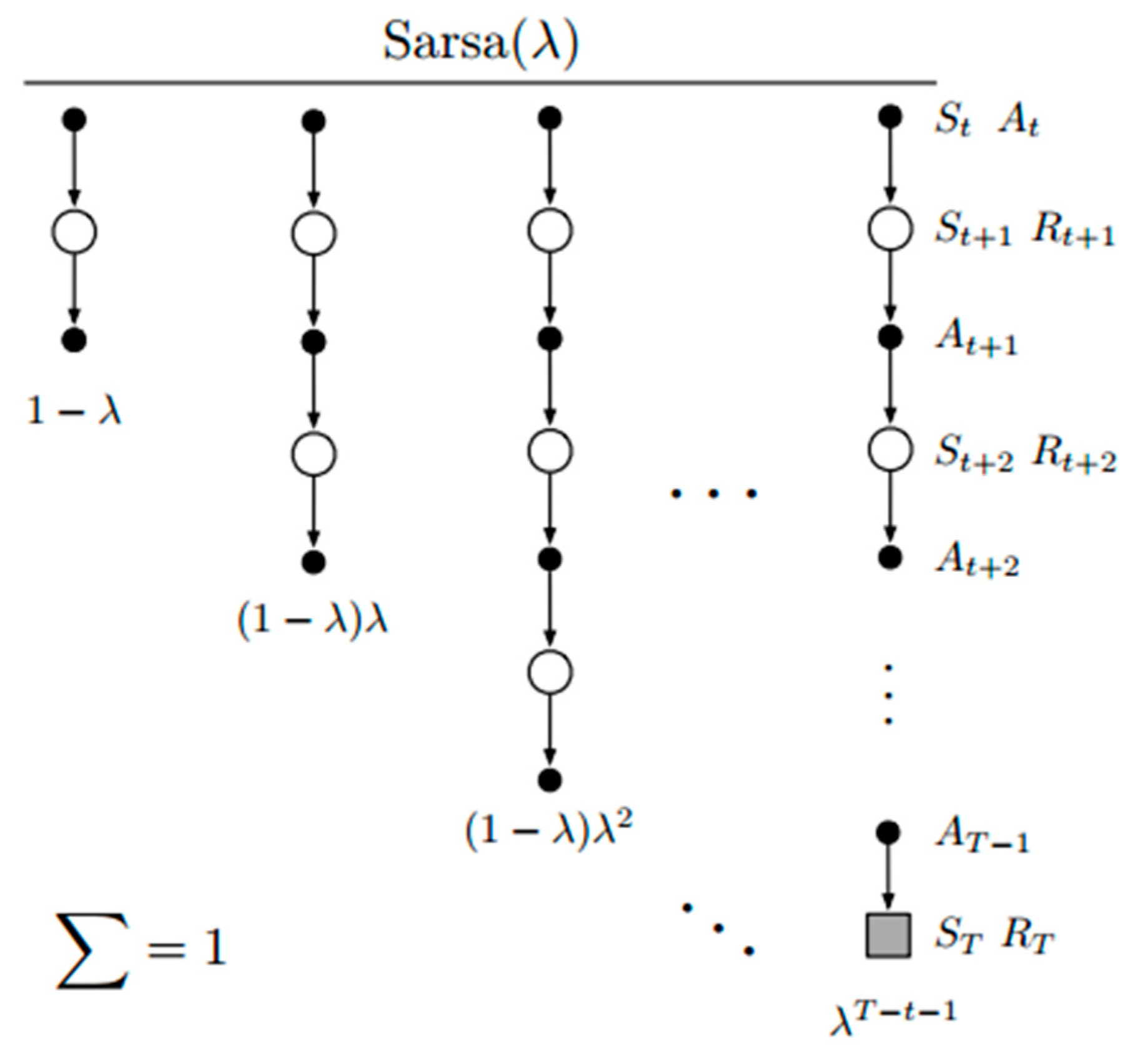
Compared with Sarsa, the Sarsa (λ) algorithm has an additional eligibility trace matrix, which is used to save every step experienced in the past. By doing so, the steps that are previously experienced are able to be updated on each iteration. To make it clearer, the Sarsa (λ) backup diagram is shown in Figure 10. The first update looks ahead one full step, to the next state-action pair, the second looks ahead two steps, to the second state-action pair, and so on. A final update is based on the complete return. The weighting of each n-step update in the λ -return is also shown in Figure 10. This approach is the theoretical forward view of the learning algorithm. For each state visited, we looked forward in time to all the future rewards and decided how best to combine them. However, Sarsa (λ) is oriented backward in time. At each moment, we looked at the current TD error and assigned it backward to each prior state according to how much that state contributed to the current eligibility trace at that time. Usually λ is set between 0 and 1, which means that more of the preceding states are changed, but each more temporally distant state is changed less (in other words, giving less credit) because the corresponding eligibility trace is smaller. Algorithm 3 shows the pseudo code for the Sarsa (λ) algorithm.
Algorithm 3. The Sarsa (λ) algorithm pseudo code.
  Algorithm : RL : Sarsa - λ   algorithm     1 . Initialize   Q ( s , a )   arbitrarily ,   for   all   s S , a A ( s )   2 . Repeat   ( for   each   episode ) :   3 .   E ( s , a ) = 0 , for   all   s S , a A ( s )     4 .   Initialize   S , A   5 .   Repeat   ( for   each   step   of   episode ) :   6 .   Take   action   A ,   observe   R , S   7 .   Choose   A   from   S   using   policy   derived   from   Q ( e . g . ,   ε g r e e d y )   8 .   δ R + γ Q ( S , A ) Q ( S , A )   9 .   E ( S , A ) E ( S , A ) + 1   10 .   For   all   s S , a A ( s )     11 .   Q ( s , a ) Q ( s , a ) + α δ E ( s , a )   12 .   E ( s , a ) γ λ E ( s , a )   13 .   S S ; A A ;   14 .   Until   S   is   terminal  

3.6. Dyna-Q Algorithm

The Dyna-Q algorithm is based on the Q-learning algorithm. It is an algorithm that combines the features of model based and model free. It learns both in the model and in the environment interaction. That is, in each iteration round, it will interact with the environment first, and update the Q function. Then, the simulation planning of the model is performed n times, and the Q function is updated correspondingly. Figure 11 illustrates the overall architecture of Dyna-Q algorithm. It can be seen that the same RL method (here the Q-learning method) is used both for learning from real experience and for planning from simulated experience. Thus, learning and planning are deeply integrated in the sense that they share almost all the same machinery, differing only in the source of their experience. Algorithm 4 shows the pseudo code for the Dyna-Q algorithm.
Algorithm 4. The Dyna-Q algorithm pseudo code.
  Algorithm : RL : Dyna - Q   algorithm     1 . Initialize   Q ( s , a )   and   M ( s , a )   for   all   s S   and   a A ( s )   2 . Do   forever :   3 .   S current   ( nonterminal )   state   4 .   A ε g r e e d y ( S , Q )   5 .   Execute   action   A ; observe   resultant   reward , R ,   and   state , S   6 .   Q ( S , A ) Q ( S , A ) + α [ R + γ max a Q ( S , a ) Q ( S , A ) ]   7 .   Model ( S , A ) R , S ( assuming   deterministic   environment )   8 .   Repeat   n   times :   9 .   S random   previously   observed   state   10 .   A random   action   previously   taken   in   S   11 .   R , S Model ( S , A )   12 .   Q ( S , A ) Q ( S , A ) + α [ R + γ max a Q ( S , a ) Q ( S , A ) ]

4. Experimental Results and Discussion

The experimental results are structured as follows: Section 4.1 shows the tracking control of the small-scale vehicle based on Q-learning, Sarsa, Sarsa (λ), and Dyna-Q at constant velocity. In Section 4.2, the Q-learning, Sarsa, and Sarsa (λ) algorithms are used to showcase the tracking behavior while learning to increment the vehicle speed. Section 4.3 shows the ultimate aim of this study, which is to enable the vehicle travelling along its centerline while learning to slow-down or accelerate adaptively according to different road conditions.

4.1. Tracking Control at Constant Vehicle Velocity

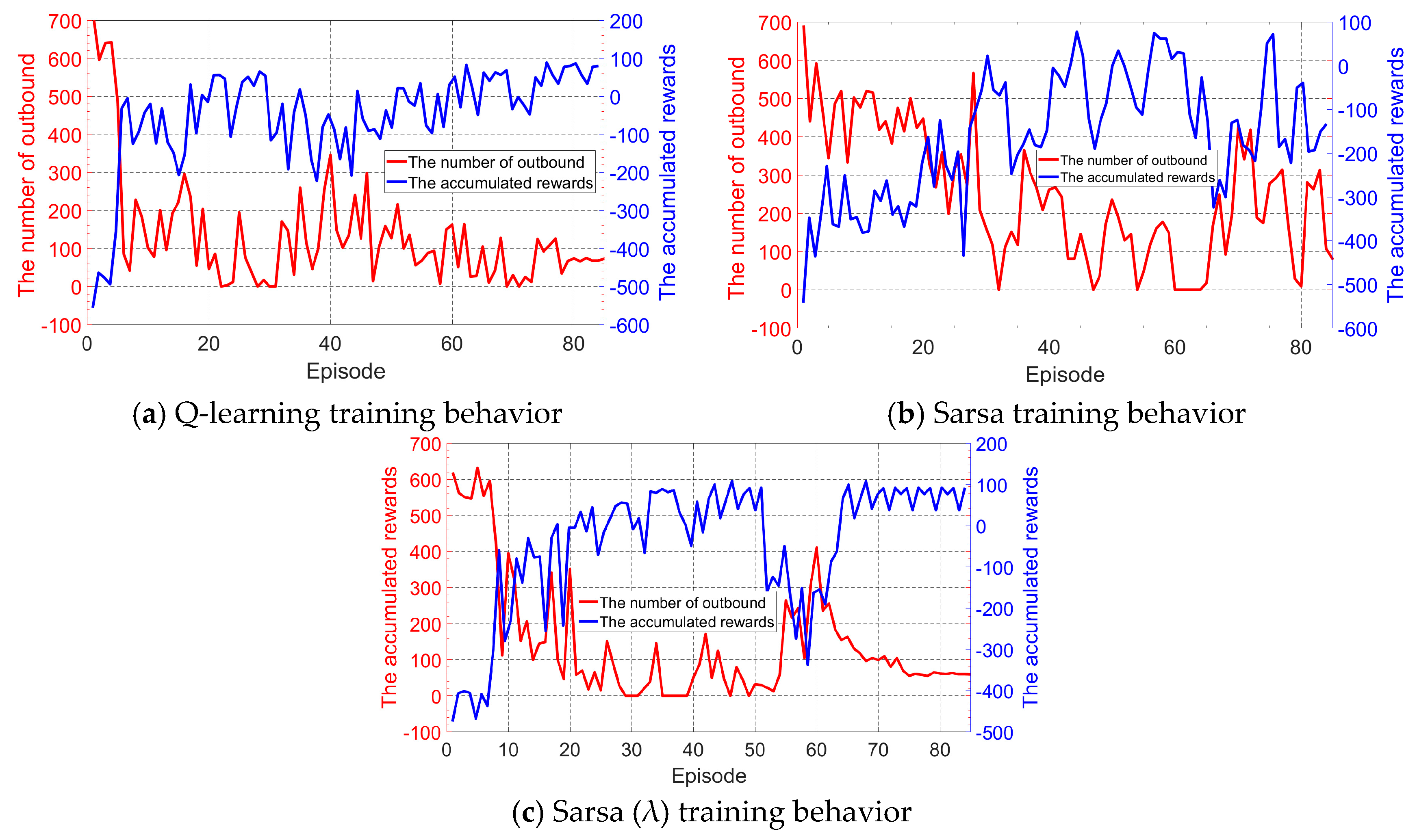
Figure 12 shows the number of outbound and the accumulated rewards per episode during the Q-learning, Sarsa, and Sarsa (λ) training process. It can be seen that all of the three RL algorithms are able to reach the convergence after a certain episode, i.e., the number of outbound per episode converges to zero and the accumulated rewards per episode converges to a certain value. But the difference between the three algorithms is also clear. For example, the training effect of the Q-learning algorithm is better than that of Sarsa. To make it clearer, The Q-learning curve can converge in a shorter time and can get more accumulated rewards in a shorter time (the final accumulated rewards are also larger). In addition, the converging speed of the Sarsa (λ) algorithm seems to be better than the Q-learning method, but only by a very small margin, and the Sarsa (λ) algorithm seems to be more stable in the training and can converge to a higher steady value in the accumulated reward figure (which corresponds to a better final control behavior) than the proposed Q-learning. From the degree of inclination of the curve, Sarsa is not as fast as the other two algorithms because of its “conservative” behavior in learning, while the backtracking learning process features of Sarsa (λ) and the courage of Q-learning in exploring movements make their learning more efficient.
When the model-free RL techniques above were compared with the model-based Dyna-Q method, Figure 13 can be drawn. It can be seen that the proposed Dyna-Q algorithm can quickly converge, just like Sarsa (λ), and the training process seems to be more stable. It indicates the superiority of the model-based approach integrates model learning and direct RL processes, although the model is only learned from real experience and gives rise to simulated experience. Furthermore, the proposed Dyna-Q algorithm, in which n was chosen to be 10, can run much faster than the proposed Sarsa (λ) method whose λ was chosen to be 0.8 (generally a good balance between the conventional Sarsa and Monte Carlo). Thus, although seen from Figure 13, the two algorithms can behave similarly after training, the proposed Dyna-Q method is more suitable to implement on real hardware, especially when the number of states and actions are discretized more finely (thus requiring more computing resources).
Table 1 compares the training process, the final control behavior, and the computational complexity between the four RL techniques. In this study, the single step calculation time is selected to represent the computational complexity (for easy comparison, the calculation time for Q-learning is used as the baseline). For Q-learning and Sarsa, as they are both a one-step TD learning method, the single step calculation time is fast. However, the computational complexity increases dramatically for Sarsa (λ) and Dyna-Q, especially when the Q table and the time of simulation planning are large. For example, if the state-action pair in the Q table was doubled, the single step calculation time of the Sarsa (λ) controller would also be doubled. That is, when the state and/or action are divided more finely, the Sarsa (λ) algorithm would not meet the real-time control requirement. From the analysis above, it can be concluded that although the proposed Q-learning algorithm has a poorer converging speed than the Sarsa (λ) and Dyna-Q algorithm, it balances the performance between the converging speed, the final control behavior, and the computational complexity, thus putting it more suitable for the first trial of industrial application.

4.2. Tracking Control While Learning to Increament the Vehicle Speed

Figure 14 shows the tracking training processes while the vehicle learns to increment speed using Q-learning, Sarsa, and Sarsa (λ). We first set the initial speed of the three algorithms to be 50% of the maximum available speed. After detecting the training converging with a good control behavior, the vehicle speed is increased by 10% of the maximum available speed automatically and this iteration stops when the learning curve vibrates (in this case, the vehicle speed of the previous iteration is determined as the maximum speed that can be achieved). In this experiment, we can see that after a certain period of training, the proposed Q-learning, Sarsa, and Sarsa (λ) algorithm can accelerate to 80%, 60%, and 90% of its maximum available speed, respectively. This indicates that the learning ability of Q-learning to adapt to different environments is stronger than that of Sarsa, and Sarsa (λ) is stronger than Q-learning.
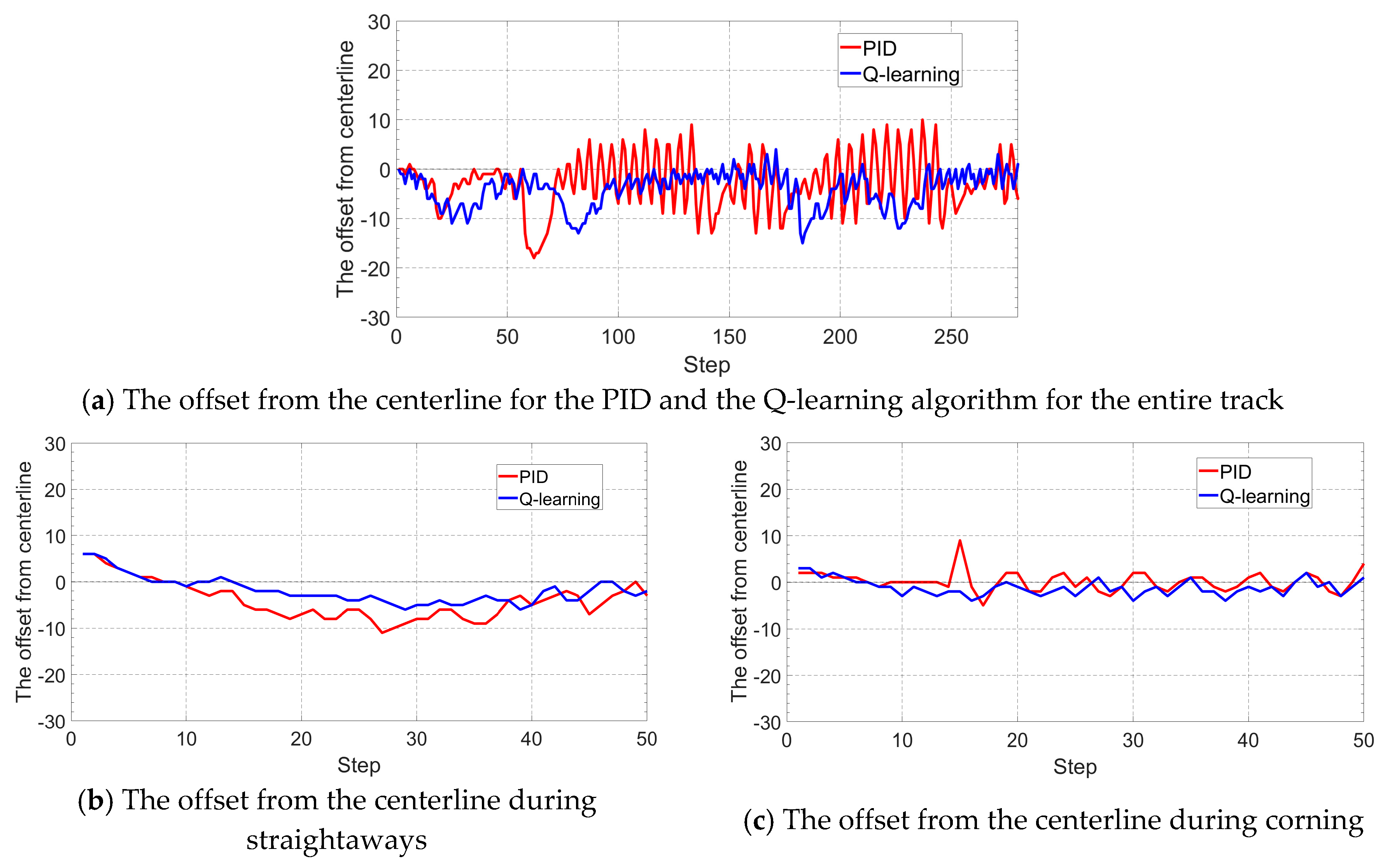
In the meanwhile, a fine-tuned PID controller has also been employed to the same task, and 70% of the maximum available speed can be achieved, indicating that the RL techniques can have a better steering control performance than that of the classical PID controller. To make it clearer, the performance of the fine-tuned PID controller is compared with the proposed Q-learning algorithm at the same vehicle speed (which corresponds to the 70% of the maximum speed). It can be seen from Figure 15 that, compared with the fine-tuned PID controller, the deviation of the vehicle position from the centerline of the trained Q-learning algorithm is much smaller throughout the entire test track, with the gap becoming bigger during corning. This is because, in general, the PID algorithm does not have a good adaptability. Its parameters may be able to maintain a good control performance in the face of a straight road, but for corners, there is no guarantee that it will still perform well. For RL, as the algorithm can have more defined states, its control strategy that maps the observed states to the control action will be more adaptive. It should also be noted here that the traditional PID algorithm requires manual adjustment of parameters so that the efficiency of algorithm tuning is low. However, RL is able to adaptively adjust the algorithm strategy in the learning process, which not only can save a lot of manpower resources, but also can more adapt to the changing environment and hardware aging over time (thus is unbiased by modelling errors).

4.3. Steering Control at Adaptive Velocity

Figure 16 shows the training process of the tracking control at adaptive cruise velocity based on Q-learning. Unlike the proposed algorithm above, which has only single output action, this section shows the ability of Q-learning with multiple actions controlled simultaneously. Quite interestingly, it can be seen that the proposed Q-learning method does not significantly increase the training time due to the increase in the number of states and actions, and still can achieve a relatively good control behavior with the number of outbound and the averaged speed per 1000 steps converging within a certain episode (after approximately 40 episodes). It should be noted that in this study, the small-scale vehicle learns to steer correctly and learns to travel with adaptive velocity almost simultaneously, which is extremely difficult for traditional PID controllers. This indicates that the Q-learning method can be an attractive alternative for complex industrial control problems (such as the self-driving control in this case) whose multiple actuators need to be regulated simultaneously.
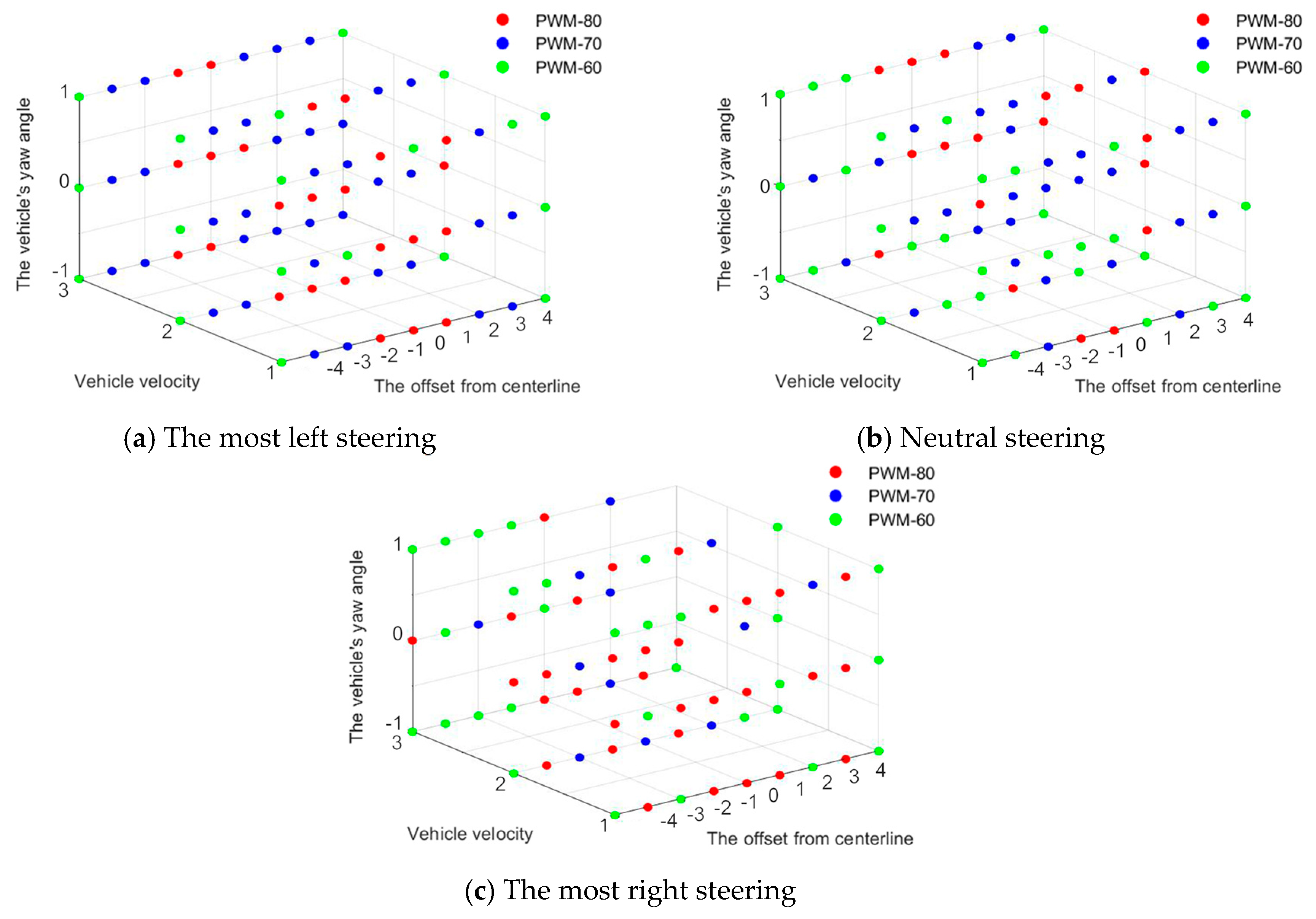
Figure 17 shows the chosen vehicle speed (indicated by motor’s pulse-width modulation: PWM) for different steering selection (in simplicity, only the most left, neural, and the most right steering are shown) at different states (namely, offset from the centerline, vehicle’s yaw angle, and current vehicle speed). Although it might be a little difficult to analyze these figures, due to its four-dimensional space, it still shows some clear trends. For example, when the vehicle is in a straight road (corresponding to the offset being 0), the vehicle is driven at the fastest speed, and when the vehicle is in a corner (corresponding to the offset being a large absolute value), the vehicle is required to be at a slower speed.
Future work may include applying deep reinforcement learning (DRL) to formulate a real-time tracking and adaptive cruise controller for the small-scale intelligent vehicle. Another interesting direction could be combining some look-ahead strategies with the proposed RL or DRL techniques to accelerate the training process and improve the final control performance. The interactions between multiple reinforcement learning based controllers, including distributed RL and hierarchical RL, will also be studied in the near future.

5. Conclusions

In this paper, three classical model-free, and a model-based RL, techniques have been employed for a small-scale vehicle with the aim to transfer the obtained knowledge to a full-scale intelligent vehicle in the near future. Unlike most of the RL-based research whose agents only interact with and learn from the virtual environments, this study directly places the small-scale vehicle in a real environment where the vehicle uses a continuous “trial-and-error” mechanism and an “exploitation and exploration” balance, in order for the parameters of the algorithm to be adjusted adaptively. In addition, the emphasis is also put on the potential industrial use by analyzing each algorithm’s training behavior and computational complexity without finely discretizing the control states and actions. The major findings are summarized as follows:
  • The Q-learning and Sarsa (λ) algorithms can achieve a better tracking behavior than the conventional Sarsa, although they all can converge within a small number of training episodes. In addition, the converging speed and the final tracking behavior of Sarsa (λ) seems to be better than Q-learning by a small margin, but Q-learning outperforms Sarsa (λ) in terms of computational complexity and thus is more suitable for the vehicle’s real time learning and control.
  • The Dyna-Q method, which can learn both in the model and in the environment interaction, performs similarly with the Sarsa (λ) algorithms, but with a significant reduction of computational time.
  • The Q-learning algorithm with a good balance between the converging speed, the computational complexity, and the final control behavior is seen to perform better compared with a fine-tune PID controller in terms of adaptability and tuning efficiency, and the Q-learning method can also be easily applied to control problems with over one control actions, putting it as more suitable for the self-driving vehicle control whose steering angle and vehicle speed needs to be regulated simultaneously.

Author Contributions

B.H. and J.L. drafted this paper and provided the overall research ideas. J.Y. provided some reinforcement learning strategy suggestion. S.L. and H.B. analyzed the data. Y.S. revised the paper. X.Y. provided some technical help.

Funding

This work is supported by the National Natural Science Foundation of China (Grants No. 51905061) in part and the Chongqing Natural Science Foundation (Grant No. cstc2019jcyj-msxmX0097) in part and the Science and Technology Research Program of Chongqing Municipal Education Commission (Grant No. KJQN201801124) in part and the Venture and Innovation Support Program for Chongqing Overseas Returners (Grant No. cx2018135) in part and the Open Project Program of the State Key Laboratory of Engines (Tianjin University) (Grant No. k2019-02) in part. Most importantly, the authors would also like to thank the anonymous reviewers for their valuable comments and suggestions.

Data Availability

The data used to support the findings of this study are available from the corresponding author upon request.

Conflicts of Interest

The authors declare no conflict of interest.

References

  1. Paden, B.; Čáp, M.; Yong, S.Z.; Yershov, D.; Frazzoli, E. A Survey of Motion Planning and Control Techniques for Self-Driving Urban Vehicles. IEEE Trans. Intell. Veh. 2016, 1, 33–55. [Google Scholar] [CrossRef]
  2. Broggi, A.; Cerri, P.; Debattisti, S.; Laghi, M.C.; Medici, P.; Molinari, D.; Panciroli, M.; Prioletti, A. PROUD—Public Road Urban Driverless-Car Test. IEEE Trans. Intell. Transp. Syst. 2015, 16, 3508–3519. [Google Scholar] [CrossRef]
  3. Li, L.; Huang, W.; Liu, Y.; Zheng, N.; Wang, F. Intelligence Testing for Autonomous Vehicles: A New Approach. IEEE Trans. Intell. Veh. 2016, 1, 158–166. [Google Scholar] [CrossRef]
  4. Xu, Z.; Wang, M.; Zhang, F.; Jin, S.; Zhang, J.; Zhao, X. Patavtt: A hardware-in-the-loop scaled platform for testing autonomous vehicle trajectory tracking. J. Adv. Transp. 2017, 1–11. [Google Scholar] [CrossRef]
  5. From the Lab to the Street: Solving the Challenge of Accelerating Automated Vehicle Testing. Available online: http://www.hitachi.com/rev/archive/2018/r2018_01/trends2/index.html/ (accessed on 1 September 2019).
  6. Ruz, M.L.; Garrido, J.; Vazquez, F.; Morilla, F. Interactive Tuning Tool of Proportional-Integral Controllers for First Order Plus Time Delay Processes. Symmetry 2018, 10, 569. [Google Scholar] [CrossRef]
  7. Liu, X.; Shi, Y.; Xu, J. Parameters Tuning Approach for Proportion Integration Differentiation Controller of Magnetorheological Fluids Brake Based on Improved Fruit Fly Optimization Algorithm. Symmetry 2017, 9, 109. [Google Scholar] [CrossRef]
  8. Chee, F.; Fernando, T.L.; Savkin, A.V.; Heeden, V.V. Expert PID Control System for Blood Glucose Control in Critically Ill Patients. IEEE Trans. Inf. Technol. Biomed. 2003, 7, 419–425. [Google Scholar] [CrossRef]
  9. Savran, A. A multivariable predictive fuzzy PID control system. Appl. Soft Comput. 2013, 13, 2658–2667. [Google Scholar] [CrossRef]
  10. Lopez_Franco, C.; Gomez-Avila, J.; Alanis, A.Y.; Arana-Daniel, N.; Villaseñor, C. Visual Servoing for an Autonomous Hexarotor Using a Neural Network Based PID Controller. Sensors 2017, 17, 1865. [Google Scholar] [CrossRef]
  11. Moriyama, K.; Nakase, K.; Mutoh, A.; Inuzuka, N. The Resilience of Cooperation in a Dilemma Game Played by Reinforcement Learning Agents. In Proceedings of the IEEE International Conference on Agents (ICA), Beijing, China, 6–9 July 2017. [Google Scholar]
  12. Meng, Q.; Tholley, I.; Chung, P.W.H. Robots learn to dance through interaction with humans. Neural Comput. Appl. 2014, 24, 117–124. [Google Scholar] [CrossRef]
  13. Zhang, Z.; Zheng, L.; Li, N.; Wang, W.; Zhong, S.; Hu, K. Minimizing mean weighted tardiness in unrelated parallel machine scheduling with reinforcement learning. Comput. Oper. Res. 2012, 39, 1315–1324. [Google Scholar] [CrossRef]
  14. Iwata, K. An Information-Theoretic Analysis of Return Maximization in Reinforcement Learning. Neural Netw. 2011, 24, 1074–1081. [Google Scholar] [CrossRef] [PubMed]
  15. Jalalimanesh, A.; Haghighi, H.S.; Ahmadi, A.; Soltani, M. Simulation-based optimization of radiotherapy: Agent-based modelling and reinforcement learning. Math. Comput. Simul. 2017, 133, 235–248. [Google Scholar] [CrossRef]
  16. Fernandez-Gauna, B.; Marques, I.; Graña, M. Undesired state-action prediction in multi-Agent reinforcement learning for linked multi-component robotic system control. Inf. Sci. 2013, 232, 309–324. [Google Scholar] [CrossRef]
  17. Sutton, R.S.; Barto, A.G. Reinforcement Learning: An Introduction, 2nd ed.; The MIT Press: Cambridge, MA, USA, 2018; pp. 97–113. [Google Scholar]
  18. Liu, T.; Zou, Y.; Liu, D.; Sun, F. Reinforcement Learning–Based Energy Management Strategy for a Hybrid Electric Tracked Vehicle. Energies 2015, 8, 7243–7260. [Google Scholar] [CrossRef]
  19. Sistani, M.B.N.; Hesari, S. Decreasing Induction Motor Loss Using Reinforcement Learning. J. Autom. Control Eng. 2016, 4, 13–17. [Google Scholar] [CrossRef]
  20. Shen, H.; Tan, Y.; Lu, J.; Wu, Q.; Qiu, Q. Achieving Autonomous Power Management Using Reinforcement Learning. ACM Trans. Des. Autom. Electron. Syst. 2013, 18, 1–24. [Google Scholar] [CrossRef]
  21. Anderlini, E.; Forehand, D.I.M.; Stansell, P.; Xiao, Q.; Abusara, M. Control of a Point Absorber using Reinforcement Learning. IEEE Trans. Sustain Energy 2016, 7, 1681–1690. [Google Scholar] [CrossRef]
  22. Sun, J.; Huang, G.; Sun, G.; Yu, H.; Sangaiah, A.K.; Chang, V. A Q-Learning-Based Approach for Deploying Dynamic Service Function Chains. Symmetry 2018, 10, 646. [Google Scholar] [CrossRef]
  23. Aissani, N.; Beldjilali, B.; Trentesaux, D. Dynamic scheduling of maintenance tasks in the petroleum industry: A reinforcement approach. Eng. Appl. Artif. Intell. 2009, 22, 1089–1103. [Google Scholar] [CrossRef]
  24. Habib, A.; Khan, M.I.; Uddin, J. Optimal Route Selection in Complex Multi-stage Supply Chain Networks using SARSA(λ). In Proceedings of the 19th International Conference on Computer and Information Technology, North South University, Dhaka, Bangladesh, 18–20 December 2016. [Google Scholar]
  25. Li, Z.; Lu, Y.; Shi, Y.; Wang, Z.; Qiao, W.; Liu, Y. A Dyna-Q-Based Solution for UAV Networks Against Smart Jamming Attacks. Symmetry 2019, 11, 617. [Google Scholar] [CrossRef]
  26. Mit-Racecar. Available online: http//www.Github.com/mit-racecar/ (accessed on 28 April 2019).
  27. Berkeley Autonomous Race Car. Available online: http//www.barc-project.com/ (accessed on 28 April 2019).
  28. Silver, D.; Schrittwieser, J.; Simonyan, K.; Antonoglou, I.; Huang, A.; Guez, A.; Hubert, T.; Baker, L.; Lai, M.; Bolton, A.; et al. Mastering the Game of Go without Human Knowledge. Nature 2017, 550, 354–359. [Google Scholar] [CrossRef] [PubMed]
  29. Pandey, P.; Pandey, D.; Kumar, S. Reinforcement Learning by Comparing Immediate Reward. Int. J. Comput. Sci. Inf. Secur. 2010, 8, 1–5. [Google Scholar]
  30. Liu, T.; Hu, X.; Li, S.E.; Cao, D. Reinforcement Learning Optimized Look-Ahead Energy Management of a Parallel Hybrid Electric Vehicle. IEEE/ASME Trans. Mechatron. 2017, 22, 1497–1507. [Google Scholar] [CrossRef]
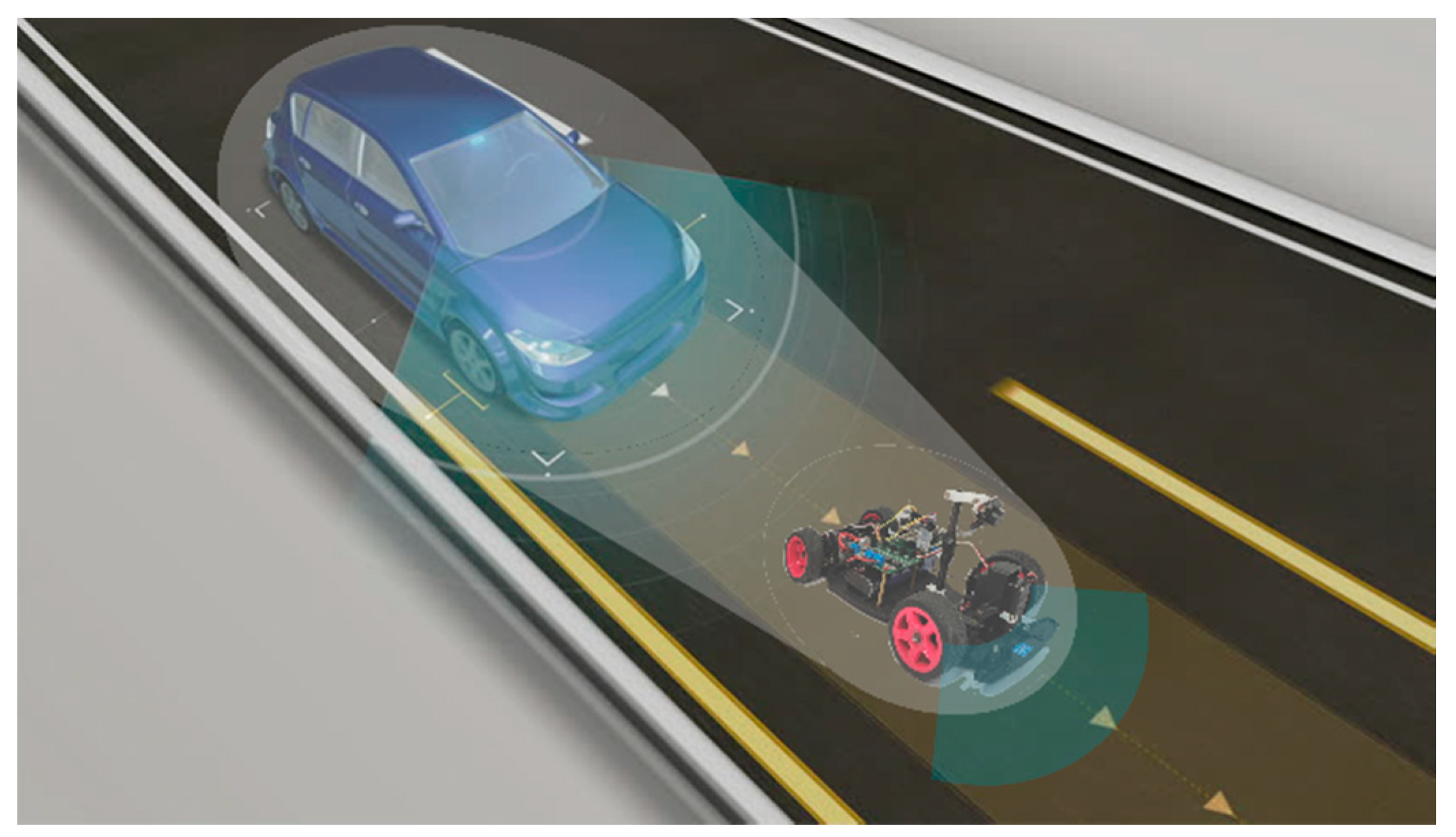
Figure 1. Small- and full- scale platform for developing and testing the intelligent algorithm for self-driving vehicles.
Symmetry 11 01139 g001
Figure 2. Basic idea and elements involved in a reinforcement learning model.
Symmetry 11 01139 g002
Figure 3. Information flow in the Dyna-Q architecture.
Symmetry 11 01139 g003
Figure 4. The small-scale intelligent vehicle platform.
Symmetry 11 01139 g004
Figure 5. Digital image processing.
Symmetry 11 01139 g005
Figure 6. Printed circuit board layout image.
Symmetry 11 01139 g006
Figure 7. The small-scale intelligent vehicle control flow chart.
Symmetry 11 01139 g007
Figure 8. System state illustration.
Symmetry 11 01139 g008
Figure 9. The Sarsa algorithm diagram.
Symmetry 11 01139 g009
Figure 10. Sarsa (λ) backup diagram.
Symmetry 11 01139 g010
Figure 11. The general Dyna-Q architecture.
Symmetry 11 01139 g011
Figure 12. The number of outbound and the accumulated rewards per episode for Q-learning, Sarsa, and Sarsa (λ).
Symmetry 11 01139 g012
Figure 13. (a) The number of outbound and (b) the accumulated rewards per episode between Dyna-Q and Sarsa (λ).
Symmetry 11 01139 g013
Figure 14. Training behavior of the tracking control while learning to increment the vehicle speed.
Symmetry 11 01139 g014
Figure 15. Tracking behavior comparison between the PID and Q-learning algorithm.
Symmetry 11 01139 g015
Figure 16. The number of outbound per episode and the averaged speed per 1000 steps.
Symmetry 11 01139 g016
Figure 17. The speed decision making algorithm for different steering gear selection.
Symmetry 11 01139 g017
Table 1. The control behavior comparison between four reinforcement learning techniques.
Q-LearningSarsaSarsa (λ)Dyna-Q
Minimum episodes to converge45502820
Final accumulated reward per episode9511657812,20412,506
Single step calculation time (%) *1001001335766
* processed after normalization.