Explicit Integrator of Runge-Kutta Type for Direct Solution of u⁽⁴⁾ = f(x, u, u′, u″)

Abstract

The primary contribution of this work is to develop direct processes of explicit Runge-Kutta type (RKT) as solutions for any fourth-order ordinary differential equation (ODEs) of the structure $u^{(4)}=f(x,u,u^{\prime },u^{″})$ and denoted as RKTF method. We presented the associated B-series and quad-colored tree theory with the aim of deriving the prerequisites of the said order. Depending on the order conditions, the method with algebraic order four with a three-stage and order five with a four-stage denoted as RKTF4 and RKTF5 are discussed, respectively. Numerical outcomes are offered to interpret the accuracy and efficacy of the new techniques via comparisons with various currently available RK techniques after converting the problems into a system of first-order ODE systems. Application of the new methods in real-life problems in ship dynamics is discussed.

1. Introduction

Fourth-order ODEs can be found in several areas of neural network engineering and applied sciences [1], fluid dynamics [2], ship dynamics [3,4,5], electric circuits [6] and beam theory [7,8]. In this article, we are dealing with development and explanation of the numerical process to solve fourth-order initial-value problems (IVPs) of the case:

$$u^{(4)}(x)=f\left(x,u(x),u^{\prime }(x),u^{″}(x)\right),$$

(1)

with initial conditions

$$u(x_0)=u_0,u^{\prime }(x_0)=u_0^{\prime },u^{″}(x_0)=u_0^{″},u^{‴}(x_0)=u_0^{‴},x\ge x_0$$

where $u,u^{\prime },u^{″},u^{‴}\in {\mathbb{R}}^d,f:\mathbb{R}\times {\mathbb{R}}^d\times {\mathbb{R}}^d\times {\mathbb{R}}^d\to {\mathbb{R}}^d$ constitute continuous vector-valued functions without third derivatives. The general fourth order needs more function evaluations to be calculated, which requires extra calculation effort and extended execution time. So we have presented the explicit formulas of RKT to solve fourth-order ODEs directly of the structure $u^{(4)}=f(x,u,u^{\prime },u^{″}).$ The numerical solution is very significant to ODEs of order four that are used in various applications since the exact solutions usually do not exist. Many researchers have used classical approaches to solve higher-order ODEs through converting them to first order system of ODEs and thus using appropriate numerical approach to this arrangement (see [9,10,11]). However, this strategy is extremely expensive because several researchers found that converting higher-order ODEs into first-order ODE systems will increase the equation count (see [7,12,13]). Consequently, more function evaluations need to be calculated, which requires into more computational effort and longer time. Many researchers have suggested direct numerical approach to more accurate results with less calculation time (see [14,15,16,17,18,19]). Furthermore, Ibrahim et al. [20] found a process by using multi-step technique which could solve stiff differential equations of order three. Jain et al. [21] developed finite difference approach to solve ODEs of order four, all the methods discussed above are multi-step in nature. On the other hand, Mechee et al. [22,23], constructed a RK-based method for solving special third-order ODEs directly. Senu et al. [24] developed embedded explicit RKT method to directly solve special ODEs of order three. Subsequently, Hussain et al. [25] proposed RKT approach for solving the aforementioned equations, except that the latter were of order four. The main purpose of this study is using quad-colored trees theory to construct one step explicit RKT approach to solve fourth-order ODEs of the structure $u^{(4)}=f(x,u,u^{\prime },u^{″})$ denoted as RKTF method.

The motivation of this study is to solve specific real-life problems such as ship dynamics which is special fourth-order ODE. Add to that, special method, RKTF will be considered that can solved directly special fourth-order ODEs which is more efficient than the general method because of the complexity of the method.

We organized this paper as follows: The idea of formulation of the RKTF methods to solve problem (1) is discussed in Section 2. B-series and associated quad-colored for RKTF methods are presented in Section 3. Section 4 investigates the construction of three- and four-staged RKTF methods of fourth and fifth orders, respectively. In the subsequent section, the efficiencies as well as accuracies the techniques will be compared against those of the existing methods. The ship dynamics problem is discussed in Section 6. Lastly conclusions and discussion are given in Section 7.

2. Formulation of the RKTF Methods

The s-stage Runge-Kutta type technique for IVP (1) of order four is given through the scheme as follows

$$\begin{array}{cc}\hfill U_i& =u_n+c_{i}h{u}_n^{\prime }+\frac{1}{2}{c}_i^2{h}^2{u}_n^{″}+\frac{1}{6}{c}_i^3{h}^3{u}_n^{‴}+h^4\sum _{j=1}^s{a}_{ij}f(x_n+c_{j}h,U_j,U_j^{\prime },U_j^{″}),\hfill \\ \hfill U_i^{\prime }& =u_n^{\prime }+c_{i}h{u}_n^{″}+\frac{1}{2}{c}_i^2{h}^2{u}_n^{‴}+h^3\sum _{j=1}^s{\overline{a}}_{ij}f(x_n+c_{j}h,U_j,U_j^{\prime },U_j^{″}),\hfill \\ \hfill U_i^{″}& =u_n^{″}+c_{i}h{u}_n^{‴}+h^2\sum _{j=1}^s{\overline{\overline{a}}}_{ij}f(x_n+c_{j}h,U_j,U_j^{\prime },U_j^{″}),\hfill \\ \hfill u_{n+1}& =u_n+h{u}_n^{\prime }+\frac{1}{2}{h}^2{u}_n^{″}+\frac{1}{6}{h}^3{u}_n^{‴}+h^4\sum _{i=1}^s{b}_{i}f(x_n+c_{i}h,U_i,U_i^{\prime },U_i^{″}),\hfill \\ \hfill u_{n+1}^{\prime }& =u_n^{\prime }+h{u}_n^{″}+\frac{1}{2}{h}^2{u}_n^{‴}+h^3\sum _{i=1}^s{b}_i^{\prime }f(x_n+c_{i}h,U_i,U_i^{\prime },U_i^{″}),\hfill \\ \hfill u_{n+1}^{″}& =u_n^{″}+h{u}_n^{‴}+h^2\sum _{i=1}^s{b}_i^{″}f(x_n+c_{i}h,U_i,U_i^{\prime },U_i^{″}),\hfill \\ \hfill u_{n+1}^{‴}& =u_n^{‴}+h\sum _{i=1}^s{b}_i^{‴}f(x_n+c_{i}h,U_i,U_i^{\prime },U_i^{″}).\hfill \end{array}$$

(2)

The assumingly real new parameters $b_i,b_i^{\prime },b_i^{″},b_i^{‴},a_{ij},{\overline{a}}_{ij},{\overline{\overline{a}}}_{ij}$ and $c_i$ of the RKTF method and used for $i,j=1,2,\dots ,s.$ The technique is explicit if $a_{ij}={\overline{a}}_{ij}={\overline{\overline{a}}}_{ij}=0$ for $i\le j$ and it is implicit otherwise.

In Kroneker’s block product, the scheme is given through as follows:

$$\begin{array}{cc}\hfill U=& e\otimes u_n+h(c\otimes u_n^{\prime })+\frac{h^2}{2}(c^2\otimes u_n^{″})+\frac{h^3}{6}(c^3\otimes u_n^{‴})+h^4(A\otimes {\mathbf{I}}_d)F(U,U^{\prime },U^{″}),\hfill \\ \hfill U^{\prime }=& e\otimes u_n^{\prime }+h(c\otimes u_n^{″})+\frac{h^2}{2}(c^2\otimes u_n^{‴})+h^3(\overline{A}\otimes {\mathbf{I}}_d)F(U,U^{\prime },U^{″}),\hfill \\ \hfill U^{″}=& e\otimes u_n^{″}+h(c\otimes u_n^{‴})+h^2(\overline{\overline{A}}\otimes {\mathbf{I}}_d)F(U,U^{\prime },U^{″}),\hfill \\ \hfill u_{n+1}& =u_n+h{u}_n^{\prime }+\frac{1}{2}{h}^2{u}_n^{″}+\frac{1}{6}{h}^3{u}_n^{‴}+h^4(b^T\otimes {\mathbf{I}}_d)F(U,U^{\prime },U^{″}),\hfill \\ \hfill u_{n+1}^{\prime }& =u_n^{\prime }+h{u}_n^{″}+\frac{1}{2}{h}^2{u}_n^{‴}+h^3(b^{{}^{\prime }T}\otimes {\mathbf{I}}_d)F(U,U^{\prime },U^{″}),\hfill \\ \hfill u_{n+1}^{″}& =u_n^{″}+h{u}_n^{‴}+h^2(b^{{}^{″}T}\otimes {\mathbf{I}}_d)F(U,U^{\prime },U^{″}),\hfill \\ \hfill u_{n+1}^{‴}& =u_n^{‴}+h(b^{{}^{‴}T}\otimes {\mathbf{I}}_d)F(U,U^{\prime },U^{″}).\hfill \end{array}$$

where, $e={[1,\dots ,1]}^T,c={[c_1,\dots ,c_s]}^T,b={[b_1,\dots ,b_s]}^T,b^{\prime }={[b_1^{\prime },\dots ,b_s^{\prime }]}^T,b^{″}={[b_1^{″},\dots ,b_s^{″}]}^T,b^{‴}={[b_1^{‴},\dots ,b_s^{‴}]}^T$, $A={\left[a_{ij}\right]}^T,$ $\overline{A}={\left[{\overline{a}}_{ij}\right]}^T,$ $\overline{\overline{A}}={\left[{\overline{\overline{a}}}_{ij}\right]}^T$ denote $s\times s$ matrices while ${\mathbf{I}}_d$ denotes $d\times d$ identity matrix. The definition of all block vectors within ${\mathbb{R}}^{s\times d}$ are as follows:

$$\begin{array}{cc}\hfill U=& {(U_1^T,\dots ,U_s^T)}^T,\hfill \\ \hfill F(U,U^{\prime },U^{″})=& {\left(f{(x_n+c_{i}h,U_i,U_i^{\prime },U_i^{″})}^T,\dots ,f{(x_n+c_{s}h,U_s,U_s^{\prime },U_s^{″})}^T\right)}^T,i=1,2,\dots ,s.\hfill \end{array}$$

The RKTF methods can be presented by the Butcher tableau of scheme (2) as follows (see Table 1):

Table 1. The Butcher tableau RKTF method.

c	A	$\overline{A}$	$\overline{\overline{A}}$
	$b^T$	$b^{{}^{\prime }T}$	$b^{{}^{″}T}$	$b^{{}^{‴}T}$

3. B-Series and Linked Quad-Colored for RKTF Methods

This section will provide the important definitions that linked relevant theorems used in this work.

Definition 1.

The RKTF formula (2) is q-ordered if for every Equation (1) of sufficient smoothness, with respect to a proposition that $u(x_n)=u_n,u^{\prime }(x_n)=u_n^{\prime },u^{″}(x_n)=u_n^{″},u^{‴}(x_n)=u_n^{‴}$, the local truncation errors of the analytic solutions as well as their derivatives must fulfil the following: (see Hussain et al. [25] and Chen et al. [26])

$$\begin{array}{c}\parallel u(x_n+h)-u_{n+1}\parallel =O(h^{q+1}),\parallel u^{\prime }(x_n+h)-u_{n+1}^{\prime }\parallel =O(h^{q+1}),\hfill \\ \parallel u^{″}(x_n+h)-u_{n+1}^{″}\parallel =O(h^{q+1}),\parallel u^{‴}(x_n+h)-u_{n+1}^{‴}\parallel =O(h^{q+1})\hfill \end{array}$$

3.1. RKTF Trees and B-Series Theory

To construct the order conditions to RKTF approach Equation (2), we are required to use autonomous formula of fourth-order IVP Equation (1)

$$u^{(4)}(x)=f\left(u(x),u^{\prime }(x),u^{″}(x)\right),$$

(3)

subject to initial prerequisites of

$$u(x_n)=u_n,u^{\prime }(x_n)=u_n^{\prime },u^{″}(x_n)=u_n^{″},u^{‴}(x_n)=u_n^{‴}.$$

The IVP (1) of order four can be defined as the autonomous form through expansion of initial-value problem (1) using one-dimensioned vector $z=x$

$$\begin{array}{c}{z}^{(4)}=0,\hfill \\ u^{(4)}=f(z,u,u^{\prime },u^{″}),\hfill \\ z(x_n):=z_n=x_n,z^{\prime }(x_n):=z_n^{\prime }=1,z^{″}(x_n):=z_n^{″}=0,z^{‴}(x_n):=z_n^{‴}=0,\hfill \\ u(x_n)=u_n,u^{\prime }(x_n)=u_n^{\prime },u^{″}(x_n)=u_n^{″},u^{‴}(x_n)=u_n^{‴}.\hfill \end{array}$$

(4)

We will obtain the same result when the RKTF approach (2) is applied to the autonomous Equation (4) and also to the non-autonomous problem (1). Thus, we want only consider the autonomous Equation (3) (see Hussain et al. [25]). Hence, to get a common method to obtain the higher-order derivatives to the analytic solutions for Equation (3), we note that the elementary differentials up to six derivatives for $u(x)$ at $x=x_0$ are given as follow:

$$\begin{array}{cc}\hfill u^{(1)}& =u^{\prime },u^{(2)}=u^{″},u^{(3)}=u^{‴},u^{(4)}=f,u^{(5)}=f_u^{\prime }{u}^{\prime }+f_{u^{\prime }}^{\prime }{u}^{″}+f_{u^{″}}^{\prime }{u}^{‴},\hfill \\ \hfill u^{(6)}& =f_{uu}^{″}(u^{\prime },u^{\prime })+2f_{u{u}^{\prime }}^{″}(u^{\prime },u^{″})+f_{u^{\prime }{u}^{\prime }}^{″}(u^{″},u^{″})+2f_{u{u}^{″}}^{″}(u^{\prime },u^{‴})+\hfill \\ & 2f_{u^{\prime }{u}^{″}}^{″}(u^{″},u^{‴})+f_{u^{″}{u}^{″}}^{″}(u^{‴},u^{‴})+f_u^{\prime }{u}^{″}+f_{u^{\prime }}^{\prime }{u}^{‴}+f_{u^{″}}^{\prime }f\hfill \end{array}$$

(5)

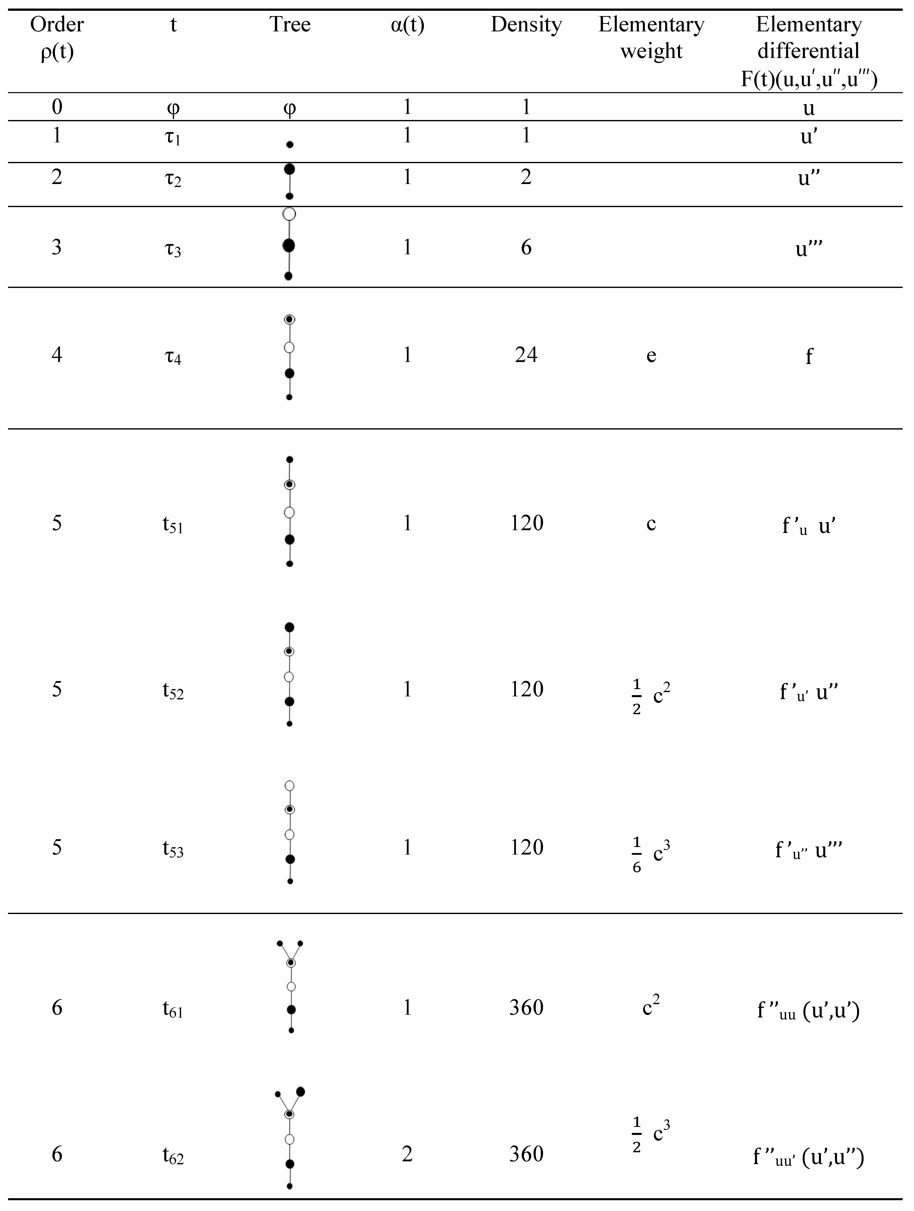
Based on Hairer et al. ([9], p. 286) a better method to tackle this issue is to use graphical exemplification indicated by quad-colored trees, in addition to some amendments to the ODEs of order four. These trees contain four kinds of; “meagre”, “black ball”, “white bal l”, as well as “black ball inside white ball” vertices both with brackets to link them. Fairly, in these trees we use the finish “meagre vertex” to denote for all $u^{\prime }$, the finish “black-ball vertices” to denote for all $u^{″}$, the finish “white ball vertex” to denote for all $u^{‴}$ and the finish “black-ball-within-white-ball vertex” to denote for all f, and all arc leaves of this vertex is the m-ordered f-derivative based on $u,u^{\prime },u^{″}$. 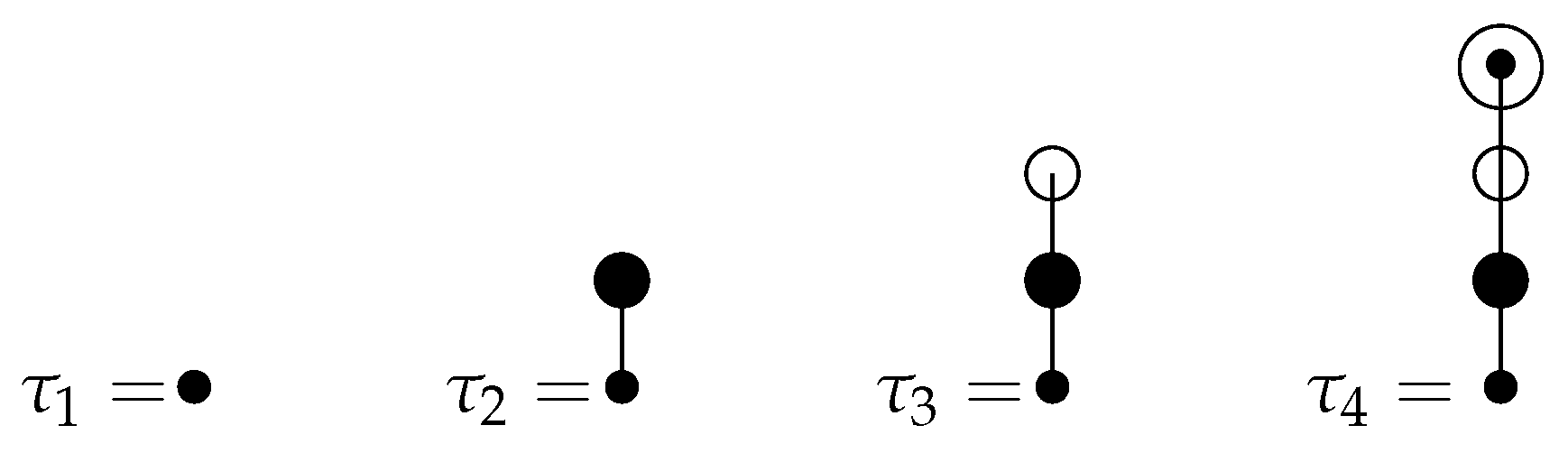The sign ${\tau }_1$ is denoted to the first algebraic order tree, the sign ${\tau }_2$ is denoted to the second algebraic order tree, the sign ${\tau }_3$ is denoted to a algebraic order three tree, while ${\tau }_4$ is denoted to the fourth algebraic order tree (see Figure 1).

Figure 1. The quad-colored trees.

Definition 2.

The repetitively explaining for the group of quad-colored trees (RT) that gives the following: (see Hussain et al. [25] and Chen et al. [26])

(a) 

The tree ${\tau }_1$ includes just one “meagre vertex” (called root) and ${\tau }_1\in RT$ and also trees mentioned above ${\tau }_2,{\tau }_3$ and ${\tau }_4$ are in $RT$.

(b) 

If $t_1,\dots ,t_r$, $t_{r+1},\dots ,t_n$, $t_{n+1},\dots ,t_m\in RT,$ then $t={[t_1,\dots ,t_r,<t_{r+1},\dots ,t_n>,<t_{n+1},\dots ,t_m>]}_4\in RT$ is the tree gained through connecting $t_1,\dots ,t_r$, $t_{r+1},\dots ,t_n$, $t_{n+1},\dots ,t_m,$ to “black ball inside white ball vertex” of the tree ${\tau }_4$ in $RT$ and the root of the “meagre vertex” ${\tau }_1$ is at the bottom. The subscript 4 is to remind that the trees of the roots of $t_1,\dots ,t_r$, $t_{r+1},\dots ,t_n$, $t_{n+1},\dots ,t_m$ to the tree ${\tau }_4$ include a series of four vertex.

To produce the quad-colored trees we shall use these basics:

(a) 

The “meagre” vertex is permanently the root.

(b) 

A “meagre” vertex has just one kid and this kid have to be “black ball”.

(c) 

A “black-ball” vertex has just one kid and this kid have to be “white ball”.

(d) 

A “white ball” vertex has just one kid and this kid have to be “black ball inside white ball vertex”.

(e) 

Each kid of a “black ball inside white ball vertex” vertex has to be “meagre”.

Definition 3.

We acquaint the order $\rho (t)$ and similarity $\sigma (t)$ functions as follows: (see Hussain et al. [25])

(a) 

$\rho ({\tau }_1)$ = 1, $\rho ({\tau }_2)$ = 2, $\rho ({\tau }_3)$ = 3, $\rho ({\tau }_4)$ = 4,

(b) 

$\sigma ({\tau }_1)$ = 1, $\sigma ({\tau }_2)$ = 1, $\sigma ({\tau }_3)$ = 1, $\sigma ({\tau }_4)$ = 1,

(c) 

If $t={[t_1,\dots ,t_r,<t_{r+1},\dots ,t_n>,<t_{n+1},\dots ,t_m>]}_4,$$\forall t\in RT$, then $\rho (t)=4+{\sum }_{i=1}^r\rho (t_i)+{\sum }_{i=r+1}^n(\rho (t_i)-1)+{\sum }_{i=n+1}^m(\rho (t_i)-2)$ and $\sigma (t)={\prod }_{i=1}^m{(\sigma (t_i))}^{{\mu }_i!}({\mu }_1!{\mu }_2!\dots ),$ where $\rho (t)$ is the number of vertices of t, $t\in RT$ and ${\mu }_1!{\mu }_2!\dots$ count equal trees between $t_1,\dots ,t_m.$

Then we can acquaint the set $S_p$ that contain all trees $RT$ of order p, where ${\mu }_i!$ is the multiplicity of $t_i$ for $i=1,\dots ,m$.

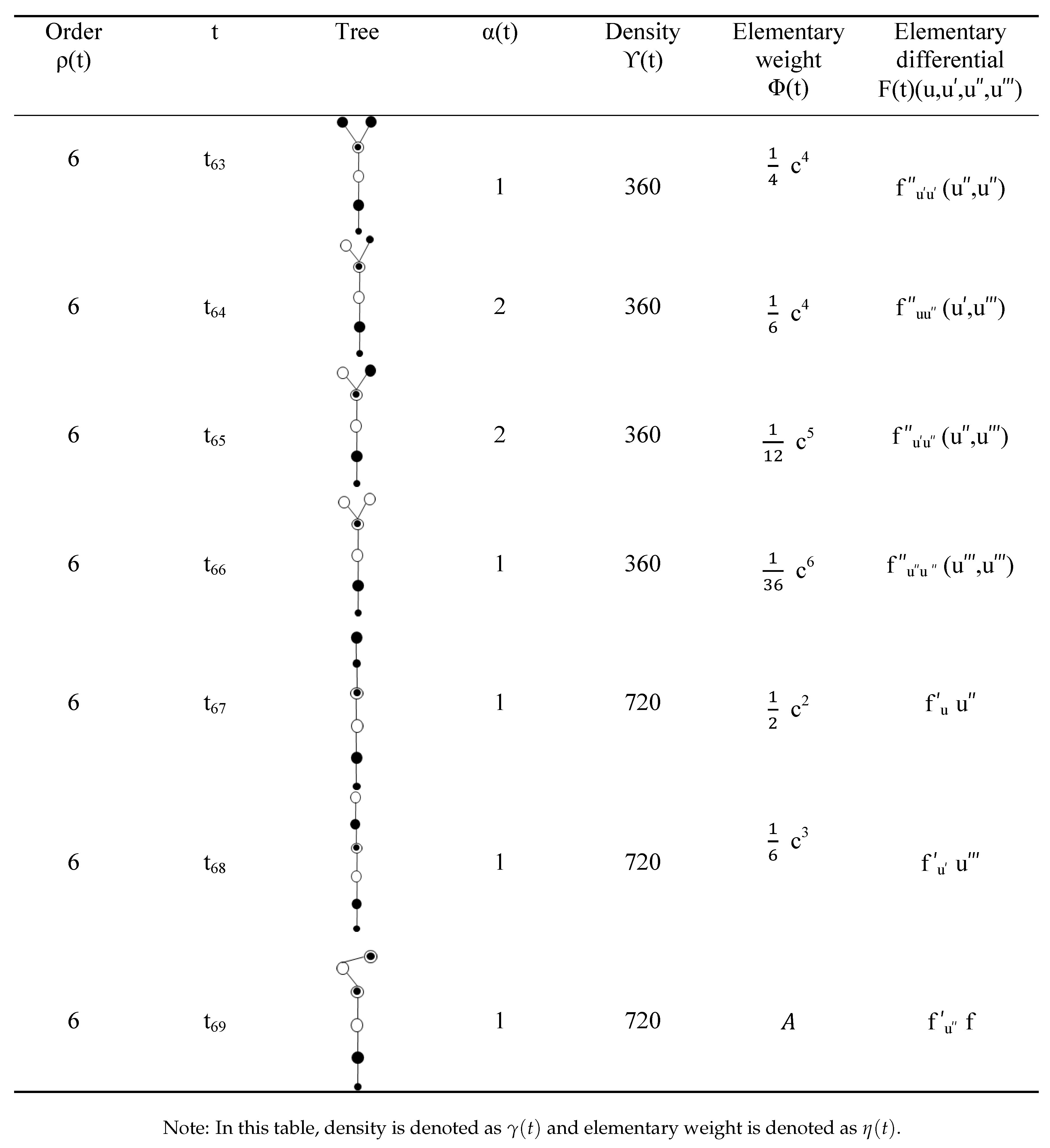
Definition 4.

The vector-valued function $F(t):{\mathbb{R}}^d\times {\mathbb{R}}^d\times {\mathbb{R}}^d\times {\mathbb{R}}^d\to {\mathbb{R}}^d$ on $RT$ is defined as the elementary differential to every tree, $tϵRT$ recursively by (see Hussain et al. [25])

(a) 

$F(\varnothing )(u,u^{\prime },u^{″},u^{‴})=u,F({\tau }_1)(u,u^{\prime },u^{″},u^{‴})=u^{\prime },F({\tau }_2)(u,u^{\prime },u^{″},u^{‴})=u^{″},F({\tau }_3)(u,u^{\prime },u^{″},u^{‴})=u^{‴},F({\tau }_4)(u,u^{\prime },u^{″},u^{‴})=f(u,u^{\prime },u^{″})$,

(b) 

$F(t)=\frac{{\partial }^{m}f}{\partial u^r\partial u^{{}^{\prime }n-r}\partial u^{{}^{″}m-n}}\left(F(t_1)(u,u^{\prime },u^{″},u^{‴}),\dots ,F(t_m)(u,u^{\prime },u^{″},u^{‴})\right)fort={[t_1,\dots ,t_r,<t_{r+1},\dots ,t_n>,<t_{n+1},\dots ,t_m>]}_4.$

Note: we denote by $<t_{r+1},\dots ,t_n>,<t_{n+1},\dots ,t_m>$ the quad-colored tree whose new roots are black ball, white ball and black ball inside white ball. (see Table 2).

Table 2. Quad-colored trees of orders up to six, elementary differentials and associated functions.

By the acquaint of B-series on the tri-colored trees in [27] and the acquaint of B-series on the root trees in ([28], p. 57), we expanded these theorems and definitions to RKTF formulas to grant the use qualifier of B-series on the group $RT$ from the quad-colored trees.

Definition 5.

For a mapping $\delta :RT\cup \{\varnothing \}\to {\mathbb{R}}^d,$ we can define format of an official series through:

$$\begin{array}{c}\hfill B(\delta ,u,u^{\prime },u^{″})=\delta (\varnothing )y+\sum _{t\in RT}\frac{h^{\rho (t)}}{\sigma (t)}\delta (t)F(t)(u,u^{\prime },u^{″},u^{‴}),\end{array}$$

(6)

is named a B-series. (see Chen et al. [26]).

We will give the fundamental lemma that provides an important role in this construct as following.

Lemma 1.

Suppose δ be a function $\delta :RT\cup \{\varnothing \}\to {\mathbb{R}}^d$ with $\delta (\varnothing )$ = 1, $\overline{\delta }$ be a function $\overline{\delta }:RT\to {\mathbb{R}}^d$ with $\overline{\delta }({\tau }_1)$ = 1 and also $\overline{\overline{\delta }}$ be a function $\overline{\overline{\delta }}:RT\to {\mathbb{R}}^d$ with $\overline{\overline{\delta }}({\tau }_2)$ = 1. Thus, $h^{4}f(B(\delta ,u,u^{\prime },u^{″}),B(\frac{\rho }{h}\overline{\delta },u,u^{\prime },u^{″}),B(\frac{\rho (\rho -1)}{h^2}\overline{\overline{\delta }},u,u^{\prime },u^{″}))$ is also B-series $h^{4}f(B(\delta ,u,u^{\prime },u^{″}),B(\frac{\rho }{h}\overline{\delta },u,u^{\prime },u^{″}),B(\frac{\rho (\rho -1)}{h^2}\overline{\overline{\delta }},u,u^{\prime },u^{″}))=$$B({\delta }^{(4)},u,u^{\prime },u^{″})$ where ${\delta }^{(4)}(\varnothing )={\delta }^{(4)}({\tau }_1)={\delta }^{(4)}({\tau }_2)={\delta }^{(4)}({\tau }_3)={\delta }^{(4)}({\tau }_4)$ = 0, ${\delta }^{(4)}({\tau }_4)$ = 1 and for $t={[t_1,\dots ,t_r,<t_{r+1},\dots ,t_n>,<t_{n+1},\dots ,t_m>]}_4,$ with $\rho (t)\ge 5,{\delta }^{(4)}(t)={\prod }_{i=1}^r\delta (t_i){\prod }_{i=r+1}^n\rho (t_i)\overline{\delta }(t_i){\prod }_{i=n+1}^m\rho (t_i)(\rho (t_i)-1)\overline{\overline{\delta }}(t_i).$

Proof. 

By assumption, $B(\delta ,u,u^{\prime },u^{″})=u+O(h)$, $B(\frac{\rho }{h}\overline{\delta },y,u^{\prime },u^{″})=u^{\prime }+O(h)$ and $B(\frac{\rho (\rho -1)}{h^2}\overline{\overline{\delta }},u,u^{\prime },u^{″})=u^{″}+O(h)$. Thus, the Taylor expansion of $f(B(\delta ,u,u^{\prime },u^{″}),B(\frac{\rho }{h}\overline{\delta },u,u^{\prime },u^{″}),B(\frac{\rho (\rho -1)}{h^2}\overline{\overline{\delta }},u,u^{\prime },u^{″}))$ shows that $f(B(\delta ,u,u^{\prime },u^{″}),B(\frac{\rho }{h}\overline{\delta },u,u^{\prime },u^{″}),B(\frac{\rho (\rho -1)}{h^2}\overline{\overline{\delta }},u,u^{\prime },u^{″}))=h^{4}f(u,u^{\prime },u^{″})+O(h^5)$ which implies that ${\delta }^{(4)}(\varnothing )={\delta }^{(4)}({\tau }_1)={\delta }^{(4)}({\tau }_2)={\delta }^{(4)}({\tau }_3)=0$, ${\delta }^{(4)}({\tau }_4)$ = 1.

Depend on the proof in Hairer et al. [28], we have

$$\begin{array}{c}{h}^{4}f(B(\delta ,u,u^{\prime },u^{″}),B(\frac{\rho }{h}\overline{\delta },y,u^{\prime },u^{″}),B(\frac{\rho (\rho -1)}{h^2}\overline{\overline{\delta }},u,u^{\prime },u^{″}))=\hfill \\ h^4\sum _{m\ge 0}\dots \sum _{n=0}^m\frac{m!}{r!(n-r)!(m-n)!}\frac{{\partial }^{m}f}{\partial u^r\partial u^{{}^{\prime }n-r}\partial u^{{}^{″}m-n}}(u,u^{\prime },u^{″}){\left(B(\delta ,u,u^{″},u^{″})-u\right)}^r\hfill \\ {\left(B(\frac{\rho }{h}\overline{\delta },u,u^{″},u^{″})-u^{\prime }\right)}^{n-r}{\left(B(\frac{\rho (\rho -1)}{h^2}\overline{\overline{\delta }},u,u^{″},u^{″})-u^{″}\right)}^{m-n}\hfill \\ =h^4\sum _{m\ge 0}\dots \sum _{n=0}^m\frac{m!}{r!(n-r)!(m-n)!}\sum _{t_1\in RT}\dots \sum _{t_r\in RT}\sum _{t_{r+1}\in RT\backslash \{{\tau }_1,{\tau }_2,{\tau }_3\}}\dots \sum _{t_n\in RT\backslash \{{\tau }_1,{\tau }_2,{\tau }_3\}}\hfill \\ \sum _{t_{n+1}\in RT\backslash \{{\tau }_1,{\tau }_2,{\tau }_3\}}\dots \sum _{t_m\in RT\backslash \{{\tau }_1,{\tau }_2,{\tau }_3\}}\frac{h^{\rho (t_1)+\rho (t_2)+\dots \rho (t_m)-(m-n)}}{\sigma (t_1)\dots \sigma (t_m)}.\rho (t_n+1)\dots \rho (t_m)\delta (t_1)\dots \hfill \\ \delta (t_r)\overline{\delta }(t_r+1)\dots \overline{\delta }(t_n)\overline{\overline{\delta }}(t_n+1)\dots \overline{\overline{\delta }}(t_m)\frac{{\partial }^{m}f}{\partial u^r\partial u^{{}^{\prime }n-r}\partial u^{{}^{″}m-n}}(u,u^{\prime },u^{″})(F(t_1)(u,u^{\prime },u^{″},u^{‴})\hfill \\ \dots F(t_m)(u,u^{\prime },u^{″},u^{‴}))=\sum _{m\ge 0}\sum _{r=0}^m\sum _{t_1\in RT}\dots \sum _{t_r\in RT}\sum _{t_{r+1}\in RT\backslash \{{\tau }_1,{\tau }_2,{\tau }_3\}}\dots \hfill \\ \sum _{t_n\in RT\backslash \{{\tau }_1,{\tau }_2,{\tau }_3\}}\sum _{t_{n+1}\in RT\backslash \{{\tau }_1,{\tau }_2,{\tau }_3\}}\dots \sum _{t_m\in RT\backslash \{{\tau }_1,{\tau }_2,{\tau }_3\}}\frac{h^{\rho (t)}}{\sigma (t)}.\frac{m!{\mu }_1!{\mu }_2!\dots {\xi }_1!{\xi }_2!\dots {\zeta }_1!{\zeta }_2!\dots }{r!(n-r)!(m-n)!}\hfill \\ \rho (t_n+1)\dots \rho (t_m)\delta (t_1)\dots \delta (t_r)\overline{\delta }(t_r+1)\dots \overline{\delta }(t_n)\overline{\overline{\delta }}(t_n+1)\dots \overline{\overline{\delta }}(t_m)F(t)(u,u^{\prime },u^{″},u^{‴})\hfill \\ =\sum _{t\in RT,\rho (t)\ge 5}\frac{h^{\rho (t)}}{\sigma (t)}\rho (t_n+1)\dots \rho (t_m)\delta (t_1)\dots \delta (t_r)\overline{\delta }(t_r+1)\dots \overline{\delta }(t_n)\overline{\overline{\delta }}(t_n+1)\dots \hfill \\ \overline{\overline{\delta }}(t_m)F(t)(u,u^{\prime },u^{″},u^{‴})\hfill \end{array}$$

where, one equality $t={[t_1,\dots ,t_r,<t_{r+1},\dots ,t_n>,<t_{n+1},\dots ,t_m>]}_4,$ and the number of methods of ordering the subtrees $t_1,\dots ,t_m$ in $t={[t_1,\dots ,t_r,<t_{r+1},\dots ,t_n>,<t_{n+1},\dots ,t_m>]}_4,$ i.e., the multiplicity of $t={[t_1,\dots ,t_r,<t_{r+1},\dots ,t_n>,<t_{n+1},\dots ,t_m>]}_4$ is $\frac{r!(q-r)!(n-q)!(m-n)!}{m!{\mu }_1!{\mu }_2!\dots {\xi }_1!{\xi }_2!\dots {\zeta }_1!{\zeta }_2!\dots }$, ${\mu }_1,{\mu }_2,\dots$ count equal trees between $t_1,\dots ,t_r$, ${\xi }_1,{\xi }_2,\dots$ count equal trees between $t_{r+1},t_{r+2},\dots ,t_n$ and ${\zeta }_1,{\zeta }_2,\dots$ count equal trees between $t_{n+1},t_{r+2},\dots ,t_m$ we get

$$\begin{array}{c}\hfill {\delta }^{(4)}=\prod _{i=1}^r\delta (t_i)\prod _{i=r+1}^n\rho (t_i)\overline{\delta }(t_i)\prod _{i=n+1}^m\rho (t_i)(\rho (t_i)-1)\overline{\overline{\delta }}(t_i).\end{array}$$

Then we have

$$\begin{array}{c}{h}^{4}f(B(\delta ,u,u^{\prime },u^{″}),B(\frac{\rho }{h}\overline{\delta },y,u^{\prime },u^{″}),B(\frac{\rho (\rho -1)}{h^2}\overline{\overline{\delta }},u,u^{\prime },u^{″}))=\hfill \\ \sum _{t\in RT}\frac{h^{\rho (t)}}{\sigma (t)}{\delta }^{(4)}F(t)(u,u^{\prime },u^{″},u^{‴})=B({\delta }^{(4)},u,u^{\prime },u^{″}).\hfill \end{array}$$

 □

Theorem 1.

Suppose that the analytic solution $u(x_0+h)$ of the form (3) is B-series, $B(e,u_0,u_0^{\prime },u_0^{″})$ with a real function e defined on $RT\cup \{\varnothing \}$. Then

$$\begin{array}{c}\hfill e(\varnothing )=1,e({\tau }_1)=1,e({\tau }_2)=\frac{1}{2},e({\tau }_3)=\frac{1}{6},e({\tau }_4)=\frac{1}{24},\end{array}$$

and for $t={[t_1,\dots ,t_r,<t_{r+1},\dots ,t_n>,<t_{n+1},\dots ,t_m>]}_4$,

$$\begin{array}{cc}\hfill e(t)& =\frac{1}{\rho (t)(\rho (t)-1)(\rho (t)-2)(\rho (t)-3)}\prod _{i=1}^{r}e(t_i)\prod _{i=r+1}^n\rho (t_i)e(t_i)\hfill \\ & \prod _{i=n+1}^m\rho (t_i)(\rho (t_i)-1)e(t_i).\hfill \end{array}$$

Proof. 

$$\begin{array}{cc}\hfill u(x_0+h)& =B(e,u_0,u_0^{\prime },u_0^{″})\hfill \\ & =e(\varnothing )u_0+he({\tau }_1)u_0^{\prime }+h^{2}e({\tau }_2)u_0^{″}+h^{3}e({\tau }_3)u_0^{‴}+h^{4}e({\tau }_4)f(u_0,u_0^{\prime },u_0^{″})\hfill \\ & +\sum _{t_{r+1}\in RT\backslash \{{\tau }_1,{\tau }_2,{\tau }_3,{\tau }_4\}}\frac{h^{\rho (t)}}{\sigma (t)}e(t)F(u_0,u_0^{\prime },u_0^{″},u_0^{‴}),\hfill \end{array}$$

Thus, the first fourth derivative of $u(x_0+h)$ is presented by

$$\begin{array}{cc}\hfill {(u(x_0+h))}^{\prime }& =\frac{d}{dh}\left[u(x_0+h)\right]=e({\tau }_1)u_0^{\prime }+2he({\tau }_2)u_0^{″}+3h^{2}e({\tau }_3)u_0^{‴}+4h^{3}e({\tau }_4)f(u_0,u_0^{\prime },u_0^{″})\hfill \\ & +\sum _{t_{r+1}\in RT\backslash \{{\tau }_1,{\tau }_2,{\tau }_3,{\tau }_4\}}\frac{\rho (t)h^{\rho (t)-1}}{\sigma (t)}e(t)F(u_0,u_0^{\prime },u_0^{″},u_0^{‴})=B(\frac{\rho e}{h},u_0,u_0^{\prime },u_0^{″}),\hfill \end{array}$$

(7)

$$\begin{array}{cc}\hfill {(u(x_0+h))}^{(2)}& =\frac{d^2}{d{h}^2}\left[u(x_0+h)\right]=2e({\tau }_2)u_0^{″}+6he({\tau }_3)u_0^{‴}+12h^{2}e({\tau }_4)f(u_0,u_0^{\prime },u_0^{″})\hfill \\ & +\sum _{t_{r+1}\in RT\backslash \{{\tau }_1,{\tau }_2,{\tau }_3,{\tau }_4\}}\frac{\rho (t)(\rho (t)-1)h^{\rho (t)-2}}{\sigma (t)}e(t)F(u_0,u_0^{\prime },u_0^{″},u_0^{‴}))\hfill \\ & =B(\frac{\rho (\rho -1)e}{h^2},u_0,u_0^{\prime },u_0^{″}),\hfill \end{array}$$

(8)

$$\begin{array}{cc}\hfill {(u(x_0+h))}^{(3)}& =\frac{d^3}{d{h}^3}\left[u(x_0+h)\right]=6e({\tau }_3)u_0^{‴}+24he({\tau }_4)f(u_0,u_0^{\prime },u_0^{″})\hfill \\ & +\sum _{t_{r+1}\in RT\backslash \{{\tau }_1,{\tau }_2,{\tau }_3,{\tau }_4\}}\frac{\rho (t)(\rho (t)-1)(\rho (t)-2)h^{\rho (t)-3}}{\sigma (t)}e(t)F(u_0,u_0^{\prime },u_0^{″},u_0^{‴})\hfill \\ & =B(\frac{\rho (\rho -1)(\rho -2)e}{h^3},u_0,u_0^{\prime },u_0^{″}),\hfill \\ \hfill {(u(x_0+h))}^{(4)}& =\frac{d^4}{d{h}^4}\left[u(x_0+h)\right]=24e({\tau }_4)f(u_0,u_0^{\prime },u_0^{″})\hfill \\ & +\sum _{t_{r+1}\in RT\backslash \{{\tau }_1,{\tau }_2,{\tau }_3,{\tau }_4\}}\frac{\rho (t)(\rho (t)-1)(\rho (t)-2)(\rho (t)-3)h^{\rho (t)-4}}{\sigma (t)}e(t)F(u_0,u_0^{\prime },u_0^{″},u_0^{‴})\hfill \\ & =B(\frac{\rho (\rho -1)(\rho -2)(\rho -3)e}{h^4},u_0,u_0^{\prime },u_0^{″}),\hfill \end{array}$$

(9)

Moreover, of Lemma 1, we have

$$\begin{array}{c}f(B(e,u,u^{\prime },u^{″}),B(\frac{\rho }{h}e,u,u^{\prime },u^{″}),B(\frac{\rho (\rho -1)}{h^2}e,u,u^{\prime },u^{″}))=e^{(4)}({\tau }_4)f(u_0,u_0^{\prime },u_0^{″})\hfill \\ +\sum _{t\in RT\backslash \{{\tau }_1,{\tau }_2,{\tau }_3,{\tau }_4\}}\frac{h^{\rho (t)-4}}{\sigma (t)}{e}^{(4)}(t)F(u_0,u_0^{\prime },u_0^{″},u_0^{‴}),\hfill \end{array}$$

(10)

where $e^{(4)}({\tau }_4)=1$ and $t={[t_1,\dots ,t_r,<t_{r+1},\dots ,t_n>,<t_{n+1},\dots ,t_m>]}_4\in RT\backslash \{{\tau }_1,{\tau }_2,{\tau }_3,{\tau }_4\}$,

$$\begin{array}{c}\hfill e^{(4)}(t)=\prod _{i=1}^{r}e(t_i)\prod _{i=r+1}^n\rho (t_i)e(t_i)\prod _{i=n+1}^m\rho (t_i)(\rho (t_i)-1)e(t_i),\end{array}$$

Inserting (9) and (10) to Equation (3), then depending on the both sides, we compare the coefficients of the same elementary differential to obtain

$$e^{}({\tau }_4)=\frac{1}{24},$$

and $t={[t_1,\dots ,t_r,<t_{r+1},\dots ,t_n>,<t_{n+1},\dots ,t_m>]}_4\in RT\backslash \{{\tau }_1,{\tau }_2,{\tau }_3,{\tau }_4\},$

$$\begin{array}{cc}\hfill e(t)& =\frac{1}{\rho (t)(\rho (t)-1)(\rho (t)-2)(\rho (t)-3)}\prod _{i=1}^{r}e(t_i)\prod _{i=r+1}^n\rho (t_i)e(t_i)\hfill \\ & \prod _{i=n+1}^m\rho (t_i)(\rho (t_i)-1)e(t_i).\hfill \end{array}$$

lastly, depending on the Taylor series expansions of $u(x_0+h)$ about $h=0,e(\varnothing )=e({\tau }_1)=1$, $e({\tau }_2)=\frac{1}{2},e({\tau }_3)=\frac{1}{6},e({\tau }_4)=\frac{1}{24}$. □

$\forall t\in RT$, we lead to write the density as follows $\gamma (t)=\frac{1}{e(t)}$ and also write non-negative integer as follows $\alpha (t)=\frac{\rho (t)!}{\sigma (t)\gamma (t)}$. Thus, from Theorem 1 we have two propositions that we will mention below.

Proposition 1.

$\forall t\in RT$, the density $\gamma (t)$ is the non-negative integer valued function on $RT$ satisfying. (see Hussain et al. [25] and Chen et al. [26])

(i) 

$\gamma ({\tau }_1)=1,\gamma ({\tau }_2)=2,\gamma ({\tau }_3)=6,\gamma ({\tau }_4)=24$,

(ii) 

$t={[t_1,\dots ,t_r,<t_{r+1},\dots ,t_n>,<t_{n+1},\dots ,t_m>]}_4\in RT$,

$$\begin{array}{c}\hfill \gamma (t)=\rho (t)(\rho (t)-1)(\rho (t)-2)(\rho (t)-3)\prod _{i=1}^r\gamma (t_i)\prod _{i=r+1}^n\frac{\gamma (t_i)}{\rho (t_i)}\prod _{i=n+1}^m\frac{\gamma (t_i)}{\rho (t_i)(\rho (t_i)-1)},\end{array}$$

Proposition 2.

$\forall t\in RT$, $\alpha (t)$ is the positive-integer satisfying. (see Chen et al. [26])

(i) 

$\alpha (t_1)=1,\alpha (t_2)=1,\alpha (t_3)=1,\alpha (t_4)=1$,

(ii) 

$t={[t_1^{{\mu }_1},\dots ,t_r^{{\mu }_r},<t_{r+1}^{{\mu }_{r+1}},\dots ,t_n^{{\mu }_n}>,,<t_{n+1}^{{\mu }_{n+1}},\dots ,t_m^{{\mu }_m}>]}_4\in RT$, with $t_1,\dots ,t_r$ distinct and $t_{r+1},\dots ,t_n$ distinct, $t_{n+1},\dots ,t_m$ distinct,

$$\begin{array}{c}\hfill \alpha (t)=(\rho (t)-4)!\prod _{i=1}^r\frac{1}{{\mu }_i!}{\left(\frac{\alpha (t_i)}{\rho (t_i)!}\right)}^{{\mu }_i}\prod _{i=r+1}^n\frac{1}{{\mu }_i!}{\left(\frac{\alpha (t_i)}{\rho (t_i)-1)!}\right)}^{{\mu }_i}\prod _{i=n+1}^m\frac{1}{{\mu }_i!}{\left(\frac{\alpha (t_i)}{\rho (t_i)-2)!}\right)}^{{\mu }_i},\end{array}$$

where ${\mu }_i$ is the multiplicity of $t_i,i=1,\dots ,m$.

Then the B-series (6) can be written as follows:

$$\begin{array}{c}\hfill B(\delta ,u,u^{\prime },u^{″})=\delta (\varnothing )y+\sum _{t\in RT}\frac{h^{\rho (t)}}{\rho (t)!}\delta (t)\gamma (t)\alpha (t)F(t)(u,u^{\prime },u^{″},u^{‴}),\end{array}$$

(11)

and $f(B(\delta ,u,u^{\prime },u^{″}),B(\frac{\rho }{h}\overline{\delta },y,u^{\prime },u^{″}),B(\frac{\rho (\rho -1)}{h^2}\overline{\overline{\delta }},u,u^{\prime },u^{″})),$ can be expressed as

$$\begin{array}{c}f(B(\delta ,u,u^{\prime },u^{″}),B(\frac{\rho }{h}\overline{\delta },y,u^{\prime },u^{″}),B(\frac{\rho (\rho -1)}{h^2}\overline{\overline{\delta }},u,u^{\prime },u^{″}))=\hfill \\ \sum _{t_{}\in RT\backslash \{{\tau }_1,{\tau }_2,{\tau }_3\}}\frac{h^{\rho (t)-4}}{\rho (t)!}{\delta }^{(4)}\gamma (t)\alpha (t)F(t)(u,u^{\prime },u^{″},u^{‴}).\hfill \end{array}$$

(12)

3.2. B-Series of the Exact Solution and Exact Derivative

Depending on the former analysis, we can present the theorem as following

Theorem 2.

The analytic solution $u(x_0+h)$ of the problem (3) and the derivative $u^{\prime }(x_0+h)$, $u^{″}(x_0+h)$, $u^{‴}(x_0+h)$ have B-series respectively as follows,

$$\begin{array}{cc}\hfill u(x_0+h)& =u_0+\sum _{t\in RT}\frac{h^{\rho (t)}}{\rho (t)!}\alpha (t)F(t)(u_0,u_0^{\prime },u_0^{″},u_0^{‴})=B\left(\frac{\alpha (t)\sigma }{\rho !},u_0,u_0^{\prime },u_0^{″}\right)\hfill \\ & =B\left(\frac{1}{\gamma (t)},u_0,u_0^{\prime },u_0^{″}\right),\hfill \end{array}$$

(13)

$$\begin{array}{cc}\hfill u^{\prime }(x_0+h)& =\sum _{t\in RT}\frac{h^{\rho (t)-1}}{(\rho (t)-1)!}\alpha (t)F(t)(u_0,u_0^{\prime },u_0^{″},u_0^{‴})=B\left(\frac{\alpha (t)\sigma }{h(\rho -1)!},u_0,u_0^{\prime },u_0^{″}\right)\hfill \\ & =B\left(\frac{\rho }{h\gamma (t)},u_0,u_0^{\prime },u_0^{″}\right),\hfill \end{array}$$

(14)

$$\begin{array}{cc}\hfill u^{″}(x_0+h)& =\sum _{t\in RT}\frac{h^{\rho (t)-2}}{(\rho (t)-2)!}\alpha (t)F(t)(u_0,u_0^{\prime },u_0^{″},u_0^{‴})=B\left(\frac{\alpha (t)\sigma }{h^2(\rho -2)!},u_0,u_0^{\prime },u_0^{″}\right)\hfill \\ & =B\left(\frac{\rho (\rho -1)}{h^2\gamma (t)},u_0,u_0^{\prime },u_0^{″}\right),\hfill \end{array}$$

(15)

$$\begin{array}{cc}\hfill u^{‴}(x_0+h)& =\sum _{t\in RT}\frac{h^{\rho (t)-3}}{(\rho (t)-3)!}\alpha (t)F(t)(u_0,u_0^{\prime },u_0^{″},u_0^{‴})=B\left(\frac{\alpha (t)\sigma }{h^3(\rho -3)!},u_0,u_0^{\prime },u_0^{″}\right)\hfill \\ & =B\left(\frac{\rho (\rho -1)(\rho -2)}{h^3\gamma (t)},u_0,u_0^{\prime },u_0^{″}\right).\hfill \end{array}$$

(16)

The proof is given by Hussain et al. [25]

3.3. B-Series of the Numerical Solution and Numerical Derivative

So as to constitute the B-series for the numerical solution $u_1$ and the numerical derivative $u_1^{\prime },u_1^{″},u_1^{‴}$ of the form (3) created by the RKTF approach (2), we suppose that $U_i$, $U_i^{\prime }$ and $U_i^{″}$ in Equation (2) can be developed as B-series $U_i=B({\psi }_i,u_0,u_0^{\prime },u_0^{″})$, $U_i^{\prime }=B(\frac{\rho }{h}\overline{{\psi }_i},u_0,u_0^{\prime },u_0^{″})$ and $U_i^{″}=B(\frac{\rho (\rho -1)}{h^2}{\overline{\overline{\psi }}}_i,u_0,u_0^{\prime },u_0^{″})$ respectively. Then the first-three equations in the scheme (2) are as follows,

$$\begin{array}{c}B({\psi }_i,u_0,u_0^{\prime },u_0^{″})=u_0+c_{i}h{u}_0^{\prime }+\frac{1}{2}{c}_i^2{h}^2{u}_0^{″}+\frac{1}{6}{c}_i^3{h}^3{u}_0^{‴}\hfill \\ +h^4\sum _{j=1}^s{a}_{ij}f\left(B({\psi }_i,u_0,u_0^{\prime },u_0^{″}),B(\frac{\rho }{h}\overline{{\psi }_i},u_0,u_0^{\prime },u_0^{″}),B(\frac{\rho (\rho -1)}{h^2}{\overline{\overline{\psi }}}_i,u_0,u_0^{\prime },u_0^{″})\right),\hfill \end{array}$$

$$\begin{array}{c}B(\frac{\rho }{h}\overline{{\psi }_i},u_0,u_0^{\prime },u_0^{″})=u_0^{\prime }+c_{i}h{u}_0^{″}+\frac{1}{2}{c}_i^2{h}^2{u}_0^{‴}\hfill \\ +h^3\sum _{j=1}^s{\overline{a}}_{ij}f\left(B({\psi }_i,u_0,u_0^{\prime },u_0^{″}),B(\frac{\rho }{h}\overline{{\psi }_i},u_0,u_0^{\prime },u_0^{″}),B(\frac{\rho (\rho -1)}{h^2}{\overline{\overline{\psi }}}_i,u_0,u_0^{\prime },u_0^{″})\right),\hfill \\ B(\frac{\rho (\rho -1)}{h^2}{\overline{\overline{\psi }}}_i,u_0,u_0^{\prime },u_0^{″})=u_0^{″}+c_{i}h{u}_0^{‴}\hfill \\ +h^2\sum _{j=1}^s{\overline{\overline{a}}}_{ij}f\left(B({\psi }_i,u_0,u_0^{\prime },u_0^{″}),B(\frac{\rho }{h}\overline{{\psi }_i},u_0,u_0^{\prime },u_0^{″}),B(\frac{\rho (\rho -1)}{h^2}{\overline{\overline{\psi }}}_i,u_0,u_0^{\prime },u_0^{″})\right),\hfill \end{array}$$

by (11) and (12) the former two equations can be presented as

$$\begin{array}{c}{\psi }_i(\varnothing )u_0+\sum _{t\in RT}\frac{h^{\rho (t)}}{\rho (t)!}{\psi }_i(t)\gamma (t)\alpha (t)F(t)(u,u^{\prime },u^{″},u^{‴})=u_0+c_{i}h{u}_0^{\prime }+\frac{1}{2}{c}_i^2{h}^2{u}_0^{″}\hfill \\ +\frac{1}{6}{c}_i^3{h}^3{u}_0^{‴}+h^4\sum _{j=1}^s\sum _{t_{}\in RT\backslash \{{\tau }_1,{\tau }_2,{\tau }_3\}}\frac{h^{\rho (t)}}{\rho (t)!}{a}_{ij}{{\psi }_j}^{(4)}\gamma (t)\alpha (t)F(t)(u_0,u_0^{\prime },u_0^{″},u_0^{‴}),\hfill \end{array}$$

$$\begin{array}{c}\sum _{t\in RT}\frac{h^{\rho (t)-1}}{(\rho (t)-1)!}\overline{{\psi }_i}(t)\gamma (t)\alpha (t)F(t)(u_0,u_0^{\prime },u_0^{″},u_0^{‴})=u_0^{\prime }+c_{i}h{u}_0^{″}+\frac{1}{2}{c}_i^2{h}^2{u}_0^{‴}+h^3\hfill \\ \sum _{j=1}^s\sum _{t_{}\in RT\backslash \{{\tau }_1,{\tau }_2,{\tau }_3\}}\frac{h^{\rho (t)-1}}{\rho (t)!}{\overline{a}}_{ij}{{\psi }_j}^{(4)}\gamma (t)\alpha (t)F(t)(u_0,u_0^{\prime },u_0^{″},u_0^{‴}),\hfill \end{array}$$

$$\begin{array}{c}\sum _{t\in RT}\frac{h^{\rho (t)-2}}{(\rho (t)-2)!}{\overline{\overline{\psi }}}_i(t)\gamma (t)\alpha (t)F(t)(u_0,u_0^{\prime },u_0^{″},u_0^{‴})=u_0^{″}+c_{i}h{u}_0^{‴}\hfill \\ h^2\sum _{j=1}^s\sum _{t_{}\in RT\backslash \{{\tau }_1,{\tau }_2,{\tau }_3\}}\frac{h^{\rho (t)-2}}{\rho (t)!}{\overline{\overline{a}}}_{ij}{{\psi }_j}^{(4)}\gamma (t)\alpha (t)F(t)(u_0,u_0^{\prime },u_0^{″},u_0^{‴}).\hfill \end{array}$$

It follows that

$$\begin{array}{c}{\psi }_i(\varnothing )=1,{\psi }_i({\tau }_1)=c_i,{\psi }_i({\tau }_2)=\frac{1}{2}{c}_i^2,{\psi }_i({\tau }_3)=\frac{1}{6}{c}_i^3,\hfill \\ {\psi }_i({\tau }_4)=\sum _{}^{}{a}_{ij}{{\psi }_j}^{(4)}({\tau }_4)=\sum _{j=1}^s{a}_{ij},\hfill \end{array}$$

(17)

$$\begin{array}{c}{\overline{\psi }}_i({\tau }_1)=1,{\overline{\psi }}_i({\tau }_2)=c_i,{\overline{\psi }}_i({\tau }_3)=\frac{1}{2}{c}_i^2,{\overline{\psi }}_i({\tau }_4)=\frac{1}{4}\sum _{j=1}^s{\overline{a}}_{ij},\hfill \\ \overline{\overline{{\psi }_i}}({\tau }_2)=1,{\overline{\overline{\psi }}}_i({\tau }_3)=c_i,{\overline{\overline{\psi }}}_i({\tau }_4)=\frac{1}{12}\sum _{}^{}{\overline{\overline{a}}}_{ij},\hfill \end{array}$$

(18)

and

$$\begin{array}{cc}\hfill {\psi }_i(t_{})& =\sum _{j=1}^s{a}_{ij}{{\psi }_j}^{(4)}(t),{\overline{\psi }}_i(t_{})=\sum _{j=1}^s\frac{{\overline{a}}_{ij}}{\rho (t)}{{\psi }_j}^{(4)}(t),{\overline{\overline{\psi }}}_i(t_{})=\sum _{j=1}^s\frac{{\overline{\overline{a}}}_{ij}}{\rho (t)(\rho (t)-1)}{{\psi }_j}^{(4)}(t),\hfill \end{array}$$

(19)

furthermore, for trees $t={[t_1,\dots ,t_r,<t_{r+1},\dots ,t_n>,<t_{n+1},\dots ,t_m>]}_4\in RT$ and $\rho (t)\ge 5$, Lemma 5 gives

$$\begin{array}{c}\hfill {{\psi }_j}^{(4)}(t)=\prod _{i=1}^r{\psi }_j(t_i)\prod _{i=r+1}^n\rho (t_i){\overline{\psi }}_j\prod _{i=n+1}^m\rho (t_i)(\rho (t_i)-1){\overline{\overline{\psi }}}_j,\end{array}$$

(20)

inserting (19) into (20) we obtain:

$$\begin{array}{c}\hfill {{\psi }_j}^{(4)}(t)=\prod _{i=1}^r\left[\sum _{k=1}^s{a}_{jk}{{\psi }_k}^{(4)}(t_i)\right]\prod _{i=r+1}^n\left[\sum _{k=1}^s{\overline{a}}_{jk}{\overline{{\psi }_k}}^{(4)}(t_i)\right]\prod _{i=n+1}^m\left[\sum _{k=1}^s{\overline{\overline{a}}}_{jk}{\overline{\overline{\psi }}}_k^{(4)}(t_i)\right].\end{array}$$

(21)

We denote ${{\psi }_j}^{(4)}(t_i)={\eta }_j(t)$, for all trees $t={[t_1,\dots ,t_r,<t_{r+1},\dots ,t_n>,<t_{n+1},\dots ,t_m>]}_4\in RT$ and $\rho (t)\ge 5$.

Thus, (21) can be written as follows,

$$\begin{array}{c}\hfill {\eta }_j(t)=\prod _{i=1}^r\left[\sum _{k=1}^s{a}_{jk}{\eta }_k(t_i)\right]\prod _{i=r+1}^n\left[\sum _{k=1}^s{\overline{a}}_{jk}\overline{{\eta }_k}(t_i)\right]\prod _{i=n+1}^m\left[\sum _{k=1}^s{\overline{\overline{a}}}_{jk}{\overline{\overline{\eta }}}_k(t_i)\right].\end{array}$$

Commonly, the next significant lemma yields the values of ${\eta }_j(\tau )$ for each tree belonging to $RT\backslash \{{\tau }_1,{\tau }_2,{\tau }_3\}$

Lemma 2.

We can compute the function ${\eta }_j(t)$ on $\in RT\backslash \{{\tau }_1,{\tau }_2,{\tau }_3\}$ recursively.

(i) 

${\eta }_j({\tau }_4)$ = 1

(ii) 

for $t={[{\tau }_1^{{\mu }_1},\dots ,t_r^{{\mu }_r},<t_{r+1}^{{\mu }_{r+1}},\dots ,t_n^{{\mu }_n}>,<t_{n+1}^{{\mu }_{n+1}},\dots ,t_m^{{\mu }_m}>]}_4\in RT$ with $t_4,\dots ,t_r$ distinct and different from ${\tau }_1,{\tau }_2,{\tau }_3,$ and $,t_{r+1},\dots ,t_n$ distinct, $t_{n+1},\dots ,t_m$ distinct,

$$\begin{array}{cc}\hfill {\eta }_i(t)& =\frac{1}{2^{{\mu }_2}{6}^{{\mu }_3}}{c}_i^{{\mu }_1+2{\mu }_2+3{\mu }_3}\prod _{k=4}^r{\left[\sum _{j=1}^s{a}_{ij}{\eta }_j(t_k)\right]}^{{\mu }_k}.\prod _{k=r+1}^n{\left[\sum _{j=1}^s{\overline{a}}_{ij}{\eta }_j(t_k)\right]}^{{\mu }_k}\hfill \\ & \prod _{k=n+1}^m{\left[\sum _{j=1}^s{\overline{\overline{a}}}_{ij}{\eta }_j(t_k)\right]}^{{\mu }_k},\hfill \end{array}$$

where, ${\mu }_1,{\mu }_2,{\mu }_3$ is the multiplicity of ${\tau }_1,{\tau }_2,{\tau }_3$ respectively and ${\mu }_k$ is the multiplicity of $t_k$ for $k=4,..,n.$

Here, we define the vector $\eta (t)={\left({\eta }_1(t),\dots ,{\eta }_s(t)\right)}^T$ for $t_{}\in RT\backslash \{{\tau }_1,{\tau }_2,{\tau }_3\}$

(i)

The initial weight linked to $u_{n+1}$ is denoted by $\phi (t)={\sum }_{}^{}{b}_i{\eta }_i(t)=b^T\eta (t)$

(ii)

${\phi }^{{}^{\prime }}(t)$ is denoted to the initial weight linked with $u_{n+1}^{\prime }$ and written as follows: ${\phi }^{\prime }(t)={\sum }_{i=1}^s{b}_i^{\prime }{\eta }_i(t)=b_i^{\prime T}\eta (t)$

(iii)

${\phi }^{″}(t)$ is denoted to the initial weight linked with $u_{n+1}^{″}$ and written as follows: ${\phi }^{″}(t)={\sum }_{i=1}^s{b}_i^{″}{\eta }_i(t)=b_i^{″T}\eta (t)$.

(iv)

${\phi }^{‴}(t)$ is denoted to the initial weight linked with $u_{n+1}^{‴}$ and written as follows: ${\phi }^{‴}(t)={\sum }_{i=1}^s{b}_i^{‴}{\eta }_i(t)=b_i^{‴T}\eta (t)$.

Theorem 3.

The numerical solution $u_1$ and the numerical derivative $u_1^{\prime },u_1^{″},u_1^{‴}$ of Equation (3) produced by the RKTF approach (2) have the following B-series

$$\begin{array}{cc}\hfill u_1(x_0+h)& =u_0+h{u}_0^{\prime }+\frac{1}{2}{h}^2{u}_0^{″}+\frac{1}{6}{h}^3{u}_0^{‴}+\sum _{t_{}\in RT\backslash \{{\tau }_1,{\tau }_2,{\tau }_3\}}\frac{h^{\rho (t)}}{\rho (t)!}\phi (t)\gamma (t)\alpha (t)F(t)(u_0,u_0^{\prime },u_0^{″},u_0^{‴}),\hfill \end{array}$$

$$\begin{array}{cc}\hfill u_1^{\prime }(x_0+h)& =u_0^{\prime }+h{u}_0^{″}+\frac{1}{2}{h}^2{u}_0^{‴}+\sum _{t_{}\in RT\backslash \{{\tau }_1,{\tau }_2,{\tau }_3\}}\frac{h^{\rho (t)-1}}{\rho (t)!}{\phi }^{\prime }(t)\gamma (t)\alpha (t)F(t)(u_0,u_0^{\prime },u_0^{″},u_0^{‴}),\hfill \\ \hfill u_1^{″}(x_0+h)& =u_0^{″}+h{u}_0^{‴}+\sum _{t_{}\in RT\backslash \{{\tau }_1,{\tau }_2,{\tau }_3\}}\frac{h^{\rho (t)-2}}{\rho (t)!}{\phi }^{″}(t)\gamma (t)\alpha (t)F(t)(u_0,u_0^{\prime },u_0^{″},u_0^{‴}),\hfill \\ \hfill u_1^{‴}(x_0+h)& =u_0^{‴}+\sum _{t_{}\in RT\backslash \{{\tau }_1,{\tau }_2,{\tau }_3\}}\frac{h^{\rho (t)-3}}{\rho (t)!}{\phi }^{‴}(t)\gamma (t)\alpha (t)F(t)(u_0,u_0^{\prime },u_0^{″},u_0^{‴}).\hfill \end{array}$$

Proof. 

By assumption, $u_i$, $u_i^{\prime }$ and $u_i^{″}$ in the scheme (2) are B-series $B({\psi }_i,u_0,u_0^{\prime },u_0^{″}),$$B(\frac{\rho }{h}\overline{{\psi }_i},u_0,u_0^{\prime },u_0^{″})$ and $B(\frac{\rho (\rho -1)}{h^2}{\overline{\overline{\psi }}}_i,u_0,u_0^{\prime },u_0^{″})$ respectively, from Lemma 5 we have

$$\begin{array}{cc}\hfill h^{4}F(u_i,u_i^{\prime },u_i^{″})=& B({\psi }_i^{(4)},u_0,u_0^{\prime },u_0^{″})=\sum _{t_{}\in RT\backslash \{{\tau }_1,{\tau }_2,{\tau }_3\}}\frac{h^{\rho (t)}}{\rho (t)!}{\psi }^{(4)}\gamma (t)\alpha (t)F(t)(u_0,u_0^{\prime },u_0^{″},u_0^{‴}).\hfill \end{array}$$

Therefore,

$$\begin{array}{cc}\hfill u_1(x_0+h)& =u_0+h{u}_0^{\prime }+\frac{1}{2}{h}^2{u}_0^{″}+\frac{1}{6}{h}^3{u}_0^{‴}+\sum _{i=1}^s{b}_{i}B({\psi }_i^{(4)},u_0,u_0^{\prime },u_0^{″})\hfill \\ \hfill =& u_0+h{u}_0^{\prime }+\frac{1}{2}{h}^2{u}_0^{″}+\frac{1}{6}{h}^3{u}_0^{‴}+\sum _{t_{}\in RT\backslash \{{\tau }_1,{\tau }_2,{\tau }_3\}}\frac{h^{\rho (t)}}{\rho (t)!}\phi (t)\gamma (t)\alpha (t)F(t)(u_0,u_0^{\prime },u_0^{″},u_0^{‴}),\hfill \\ \hfill u_1^{\prime }(x_0+h)& =u_0^{\prime }+h{u}_0^{″}+\frac{1}{2}{h}^2{u}_0^{‴}+\frac{1}{h}\sum _{i=1}^s{b}_i^{\prime }B({\psi }_i^{(4)},u_0,u_0^{\prime },u_0^{″})\hfill \\ & =u_0^{\prime }+h{u}_0^{″}+\frac{1}{2}{h}^2{u}_0^{‴}+\sum _{t_{}\in RT\backslash \{{\tau }_1,{\tau }_2,{\tau }_3\}}\frac{h^{\rho (t)-1}}{\rho (t)!}{\phi }^{\prime }(t)\gamma (t)\alpha (t)F(t)(u_0,u_0^{\prime },u_0^{″},u_0^{‴}),\hfill \\ \hfill u_1^{″}(x_0+h)& =u_0^{″}+h{u}_0^{‴}+\frac{1}{h^2}\sum _{i=1}^s{b}_i^{″}B({\psi }_i^{(4)},u_0,u_0^{\prime },u_0^{″})\hfill \\ & =u_0^{″}+h{u}_0^{‴}+\sum _{t_{}\in RT\backslash \{{\tau }_1,{\tau }_2,{\tau }_3\}}\frac{h^{\rho (t)-2}}{\rho (t)!}{\phi }^{″}(t)\gamma (t)\alpha (t)F(t)(u_0,u_0^{\prime },u_0^{″},u_0^{‴}),\hfill \\ \hfill u_1^{‴}(x_0+h)& =u_0^{‴}+\frac{1}{h^3}\sum _{i=1}^s{b}_i^{‴}B({\psi }_i^{(4)},u_0,u_0^{\prime },u_0^{″})\hfill \\ & =u_0^{‴}+\sum _{t_{}\in RT\backslash \{{\tau }_1,{\tau }_2,{\tau }_3\}}\frac{h^{\rho (t)-3}}{\rho (t)!}{\phi }^{‴}(t)\gamma (t)\alpha (t)F(t)(u_0,u_0^{\prime },u_0^{″},u_0^{‴}).\hfill \end{array}$$

 □

3.4. Algebraic Order Conditions

Through Theorem 1 and 3, we arrived at the major goal of this study.

Theorem 4.

The RKTF method (2) has order $q(4\le q)$ if and only if the following conditions are satisfied as given in Hussain et al. [25])

(i) 

$\phi (t)=\frac{1}{\gamma (t)},\rho (t)\le q,$

(ii) 

${\phi }^{\prime }(t)=\frac{\rho (t)}{\gamma (t)},\rho (t)\le q+1,$

(iii) 

${\phi }^{″}(t)=\frac{\rho (t)(\rho (t)-1)}{\gamma (t)},\rho (t)\le q+2,$

(iv) 

${\phi }^{‴}(t)=\frac{\rho (t)(\rho (t)-1)(\rho (t)-2)}{\gamma (t)},\rho (t)\le q+3.$

Corollary 1.

(see Hussain et al. [25]). Assume that

$$\begin{array}{cc}\hfill t^{\ast }=& {[{\tau }_1^{{\mu }_1+2{\mu }_2+3{\mu }_3},t_4^{{\mu }_4},\dots ,t_r^{{\mu }_r},<t_{r+1}^{{\mu }_{r+1}},\dots ,t_n^{{\mu }_n}>,<t_{n+1}^{{\mu }_{n+1}},\dots ,t_m^{{\mu }_m}>]}_4,\hfill \\ \hfill \widehat{t}=& {[{\tau }_1^{{\mu }_1},{\tau }_2^{{\mu }_2},{\tau }_3^{{\mu }_3},t_4^{{\mu }_4},\dots ,t_r^{{\mu }_r},<t_{r+1}^{{\mu }_{r+1}},\dots ,t_n^{{\mu }_n}>,<t_{n+1}^{{\mu }_{n+1}},\dots ,t_m^{{\mu }_m}>]}_4\hfill \end{array}$$

where $t_4,\dots ,t_r$ are distinct and different from ${\tau }_1,{\tau }_2$ and ${\tau }_3$ and $t_{r+1},\dots ,t_n$, $t_{n+1},\dots ,t_m$ are distinct. Then

$$\begin{array}{cc}\hfill {\eta }_i(\widehat{t})=& \frac{1}{2^{{\mu }_2}{6}^{{\mu }_3}}{\eta }_i(t^{\ast }),\rho (\widehat{t})={\rho }_i(t^{\ast }),\gamma (\widehat{t})=2^{{\mu }_2}{6}^{{\mu }_3}\gamma (t^{\ast }).\hfill \end{array}$$

Based on Corollary 1 assuming that the $t^{\ast }$ and $\widehat{t}$ trees grant the same order conditions, then these trees are equivalent. Thus, we can delete some trees since they are equivalent. For example, in Table 2 trees $t_{61}$ and $t_{68}$ of sixth-order are equivalent.

Based on Theorem 4 and Corollary 1, the algebraic order conditions up to order six for the RKTF formula can be presented as follows:

order 1:

$$b^{{}^{‴}T}e=1.$$

(22)

order 2:

$$b^{{}^{‴}T}c=\frac{1}{2},b^{{}^{″}T}e=\frac{1}{2}.$$

(23)

order 3:

$$b^{{}^{‴}T}{c}^2=\frac{1}{3},b^{{}^{‴}T}\overline{\overline{A}}=\frac{1}{6},b^{{}^{″}T}c=\frac{1}{6},b^{{}^{\prime }T}e=\frac{1}{6}.$$

(24)

order 4:

$$\begin{array}{c}{b}^{{}^{‴}T}{c}^3=\frac{1}{4},b^{{}^{‴}T}\overline{A}=\frac{1}{24},b^{{}^{‴}T}(c.\overline{\overline{A}}e)=\frac{1}{8},b^{{}^{‴}T}\overline{\overline{A}}c=\frac{1}{24},\hfill \\ b^{{}^{″}T}{c}^2=\frac{1}{12},b^{{}^{″}T}\overline{\overline{A}}=\frac{1}{24},b^{{}^{\prime }T}c=\frac{1}{24},b^{T}e=\frac{1}{24}.\hfill \end{array}$$

(25)

order 5:

$$\begin{array}{c}{b}^{{}^{‴}T}{c}^4=\frac{1}{5},b^{{}^{‴}T}A=\frac{1}{120},b^{{}^{‴}T}\overline{A}c=\frac{1}{120},b^{{}^{‴}T}c.\overline{A}e=\frac{1}{30},b^{{}^{‴}T}\overline{\overline{A}}{c}^2=\frac{1}{60},\hfill \\ b^{{}^{‴}T}(c^2.\overline{\overline{A}})=\frac{1}{10},b^{{}^{‴}T}(c.\overline{\overline{A}}c)=\frac{1}{30},b^{{}^{″}T}{c}^3=\frac{1}{20},b^{{}^{″}T}\overline{A}=\frac{1}{120},b^{{}^{″}T}(c.\overline{\overline{A}}e)=\frac{1}{40},\hfill \\ b^{{}^{″}T}\overline{\overline{A}}c=\frac{1}{120},b^{{}^{\prime }T}{c}^2=\frac{1}{60},b^{{}^{\prime }T}\overline{\overline{A}}=\frac{1}{120},b^{T}c=\frac{1}{120}.\hfill \end{array}$$

(26)

order 6:

$$\begin{array}{c}{b}^{{}^{‴}T}{c}^5=\frac{1}{6},b^{{}^{‴}T}Ac=\frac{1}{720},b^{{}^{‴}T}(c.Ae)=\frac{1}{144},b^{{}^{‴}T}\overline{A}{c}^2=\frac{1}{360},\hfill \\ b^{{}^{‴}T}(c.\overline{\overline{A}}{c}^2)=\frac{1}{72},b^{{}^{‴}T}(\overline{A}{c}^2)=\frac{1}{360},b^{{}^{‴}T}(c^2.\overline{A}e)=\frac{1}{36},\hfill \\ b^{{}^{‴}T}(c.\overline{A}c)=\frac{1}{144},b^{{}^{‴}T}(c^3.\overline{\overline{A}}e)=\frac{1}{12},b^{{}^{‴}T}\overline{\overline{A}}{c}^3=\frac{1}{120},\hfill \\ b^{{}^{‴}T}(c.\overline{\overline{A}}{c}^2)=\frac{1}{144},b^{{}^{‴}T}(c^2.\overline{\overline{A}}c)=\frac{1}{36},b^{{}^{″}T}(c.\overline{\overline{A}}c)=\frac{1}{180},b^{{}^{″}T}{c}^4=\frac{1}{30},\hfill \\ b^{{}^{″}T}A=\frac{1}{720},b^{{}^{″}T}\overline{A}c=\frac{1}{720},b^{{}^{″}T}(c.\overline{A}e)=\frac{1}{180},b^{{}^{″}T}\overline{\overline{A}}{c}^2=\frac{1}{360},\hfill \\ b^{{}^{″}T}(c^2.\overline{\overline{A}}e)=\frac{1}{60},b^{{}^{\prime }T}{c}^3=\frac{1}{120},b^{{}^{\prime }T}\overline{A}=\frac{1}{720},b^{{}^{\prime }T}(c.\overline{\overline{A}}e)=\frac{1}{240},\hfill \\ b^{{}^{\prime }T}\overline{\overline{A}}c=\frac{1}{720},b^T\overline{\overline{A}}=\frac{1}{720},b^T{c}^2=\frac{1}{360}.\hfill \end{array}$$

(27)

The following simplifying assumption is used to reduce the number of equations to be solved: $\sum {\overline{\overline{a}}}_{ij}=\frac{c_i^2}{2}.$

3.5. Zero-Stability of the New Method

Here, we will discuss the zero-stability of the new techniques. It is stable at zero significance to prove the convergence of multi-step techniques and stability (see [10,11]). In [29], also discussed on the zero-stability to obtain the upper boundedness of the multi-steps methods. Now, the first characteristic polynomial for the RKTF method for Equation (2) is based on the following equation:

$$\left[\begin{array}{cccc}1& 0& 0& 0\\ 0& 1& 0& 0\\ 0& 0& 1& 0\\ 0& 0& 0& 1\end{array}\right]\left[\begin{array}{c}{u}_{n+1}\\ h{u}_{n+1}^{\prime }\\ h^2{u}_{n+1}^{″}\\ h^3{u}_{n+1}^{‴}\end{array}\right]=\left[\begin{array}{cccc}1& 1& \frac{1}{2}& \frac{1}{6}\\ 0& 1& 1& \frac{1}{2}\\ 0& 0& 1& 1\\ 0& 0& 0& 1\end{array}\right]\left[\begin{array}{c}{u}_n\\ h{u}_n^{\prime }\\ h^2{u}_n^{″}\\ h^3{u}_n^{‴}\end{array}\right],$$

where $I=\left[\begin{array}{cccc}1& 0& 0& 0\\ 0& 1& 0& 0\\ 0& 0& 1& 0\\ 0& 0& 0& 1\end{array}\right]$ is the identity matrix coefficient of $u_{n+1},h{u}_{n+1}^{\prime },h^2{u}_{n+1}^{″}$ and $h^3{u}_{n+1}^{‴}$ and $A=\left[\begin{array}{cccc}1& 1& \frac{1}{2}& \frac{1}{6}\\ 0& 1& 1& \frac{1}{2}\\ 0& 0& 1& 1\\ 0& 0& 0& 1\end{array}\right]$ is matrix coefficient of $u_n,h{u}_n^{\prime }$, $h^2{u}_n^{″}$ and $h^3{u}_n^{‴}$, respectively.

Then, the first characteristic polynomial of new methods is

$$\rho (\zeta )=det[I\zeta -A]=\left|\begin{array}{cccc}\zeta -1& -1& -\frac{1}{2}& -\frac{1}{6}\\ 0& \zeta -1& -1& -\frac{1}{2}\\ 0& 0& \zeta -1& -1\\ 0& 0& 0& \zeta -1\end{array}\right|.$$

thus, $\rho (\zeta )={(\zeta -1)}^4.$ By solving the characteristic polynomial, we obtain the roots, $\zeta$ = 1, 1, 1, 1. Therefore, the RKTF methods is zero stable since the roots of the characteristic polynomial have modulus less than or equal to one. The RKTF is consistent because the RKTF has order $p\ge 4.$ This property, with the zero stable of the methods, implies the convergence of the RKT method.

4. Construction of the RKTF Methods

According the order conditions stated in Section 3.4 before we proceed to construct explicit RKTF methods. The local truncated error for the q order RKTF technique is defined as follows:

$$\begin{array}{c}\hfill \parallel L_g^{(q+1)}{\parallel }_2={\left(\sum _{i=1}^{n_{q+1}}{\left(L_i^{(q+1)}\right)}^2+\sum _{i=1}^{n_{q+1}^{\prime }}{\left(L_i^{\prime }{}^{(q+1)}\right)}^2+\sum _{i=1}^{n_{q+1}^{″}}{\left(L_i^{″}{}^{(q+1)}\right)}^2+\sum _{i=1}^{n_{q+1}^{‴}}{\left(L_i^{‴}{}^{(q+1)}\right)}^2\right)}^{\frac{1}{2}}\end{array}$$

(28)

where $L^{(q+1)},L^{\prime }{}^{(q+1)},L^{″}{}^{(q+1)}$ and $L^{‴}{}^{(q+1)}$ are the local truncation error terms for $u,u^{\prime },u^{″}$ and $u^{‴}$ respectively, $L_g{}^{(q+1)}$ is the global local truncation error.

4.1. A Three-Stage Fourth-Order RKTF Method

In this subsection the derivation of the three-stage RKTF technique of order four by using the algebraic order conditions up to order four and simplifying assumption $\sum {\overline{\overline{a}}}_{ij}=\frac{c_i^2}{2}$ will be considered. The resulting system consists of 15 nonlinear equations with 23 unknown variables, solving the system simultaneously and the family of solution in terms of $a_{21},a_{31},a_{32},{\overline{a}}_{32},b_2$, $c_3$ and letting ${\overline{a}}_{21}=0,b_3=0,$ and $b_3^{\prime }=0$ are given as follows:

$$\begin{array}{c}{\overline{a}}_{31}=-{\overline{a}}_{32}+\frac{3}{4}{c}_3-2{c_3}^2+\frac{3}{2}{c_3}^3,\hfill \\ {\overline{\overline{a}}}_{21}=\frac{{\left(-3+4c_3\right)}^2}{8{\left(-2+3c_3\right)}^2},{\overline{\overline{a}}}_{31}=-\frac{c_3\left(14c_3-20{c_3}^2-3+9{c_3}^3\right)}{-3+4c_3},\hfill \\ {\overline{\overline{a}}}_{32}=\frac{\left(3-8c_3+6{c_3}^2\right)c_3\left(-2+3c_3\right)}{2(-3+4c_3)},b_1=\frac{1}{24}-b_2,b_1^{\prime }=\frac{-4+5c_3}{12(-3+4c_3)},\hfill \\ b_2^{\prime }=\frac{-2+3c_3}{12(-3+4c_3)},b_1^{″}=\frac{6{c_3}^2-6c_3+1}{6\left(-3+4c_3\right)c_3},b_2^{″}=\frac{\left(2-7c_3+6{c_3}^2\right)\left(-2+3c_3\right)}{3\left(3-8c_3+6{c_3}^2\right)\left(-3+4c_3\right)},\hfill \\ b_3^{″}=\frac{-(-1+c_3)}{6\left(3-8c_3+6{c_3}^2\right)c_3},b_1^{‴}=\frac{6{c_3}^2-6c_3+1}{6\left(-3+4c_3\right)c_3},b_2^{‴}=\frac{2\left(4-12c_3+9{c_3}^2\right)\left(-2+3c_3\right)}{3\left(3-8c_3+6{c_3}^2\right)\left(-3+4c_3\right)},\hfill \\ b_3^{‴}=\frac{1}{6\left(3-8c_3+6{c_3}^2\right)c_3},c_2=\frac{-3+4c_3}{2(-2+3c_3)}.\hfill \end{array}$$

Next, we minimize the truncation error term by using minimize command in Maple. Thus, for the optimized value of coefficients in fractional form we chose $a_{21}=-\frac{23}{50}$, $a_{31}=\frac{8}{25}$, $a_{32}=\frac{8}{25}$, ${\overline{a}}_{32}=\frac{3}{50}$, $c_3=\frac{21}{25}$ and $b_2=\frac{1}{50}$ with these values $\parallel {\tau }_g^{(5)}{\parallel }_2=7.98593\times {10}^{-3}$. Finally, all the parameters of three-stage fourth-order RKTF approach that will be denoted as RKTF4 can be written as follows (see Table 3):

Table 3. The RKTF4 Method.

$\begin{array}{c}0\hfill \end{array}$

$\begin{array}{c}0\hfill \end{array}$

$\begin{array}{c}0\hfill \end{array}$

$\begin{array}{c}0\hfill \end{array}$

$\begin{array}{c}\frac{9}{26}\hfill \end{array}$

$\begin{array}{c}-\frac{23}{50}\hfill \end{array}$

$\begin{array}{c}0\hfill \end{array}$

$\begin{array}{c}0\hfill \end{array}$

$\begin{array}{c}0\hfill \end{array}$

$\begin{array}{c}\frac{81}{1352}\hfill \end{array}$

$\begin{array}{c}0\hfill \end{array}$

$\begin{array}{c}\frac{21}{25}\hfill \end{array}$

$\begin{array}{c}\frac{8}{25}\hfill \end{array}$

$\begin{array}{c}\frac{8}{25}\hfill \end{array}$

$\begin{array}{c}0\hfill \end{array}$

$\begin{array}{c}\frac{2991}{\mathrm{62,500}}\hfill \end{array}$

$\begin{array}{c}\frac{3}{50}\hfill \end{array}$

$\begin{array}{c}0\hfill \end{array}$

$\begin{array}{c}\frac{644}{\mathrm{15,625}}\hfill \end{array}$

$\begin{array}{c}\frac{9737}{\mathrm{31,250}}\hfill \end{array}$

$\begin{array}{c}0\hfill \end{array}$

$\begin{array}{c}\frac{13}{600}\hfill \end{array}$

$\begin{array}{c}\frac{1}{50}\hfill \end{array}$

$\begin{array}{c}0\hfill \end{array}$

$\begin{array}{c}\frac{5}{108}\hfill \end{array}$

$\begin{array}{c}\frac{13}{108}\hfill \end{array}$

$\begin{array}{c}0\hfill \end{array}$

$\begin{array}{c}\frac{121}{1134}\hfill \end{array}$

$\begin{array}{c}\frac{2873}{8667}\hfill \end{array}$

$\begin{array}{c}\frac{1250}{20223}\hfill \end{array}$

$\begin{array}{c}\frac{121}{1134}\hfill \end{array}$

$\begin{array}{c}\frac{4394}{8667}\hfill \end{array}$

$\begin{array}{c}\frac{\mathrm{15,625}}{\mathrm{40,446}}\hfill \end{array}$

4.2. A Four-Stage RKTF Method of Order Five

For four-stage RKTF technique of order five, the algebraic conditions up to order five will be solved. The resulting system consists of 29 nonlinear equations with 37 unknown variables, solving the system together will give a family of solution with 11 free parameters of $a_{21}$, $a_{32}$, $a_{42}$, $a_{43}$, ${\overline{a}}_{21}$, ${\overline{a}}_{42}$, ${\overline{a}}_{43}$, $b_4^{\prime }$, $c_2$, $b_3$ and $b_4$ are given as follows:

$$\begin{array}{cc}\hfill {\overline{a}}_{31}& =\frac{1}{10\left(16{c_2}^2-8c_2+1\right)\left(5c_2-4\right){\left(4c_2-1\right)}^3}(50000{c_2}^6{\overline{a}}_{4,2}-880{c_2}^5-1040{c_2}^2{\overline{a}}_{2,1}-18750{c_2}^3{\overline{a}}_{4,2}\hfill \\ & +11250{c_2}^3{\overline{a}}_{4,3}+800{c_2}^3{\overline{a}}_{2,1}+66250{c_2}^4{\overline{a}}_{4,2}-21250{c_2}^4{\overline{a}}_{4,3}-97500{c_2}^5{\overline{a}}_{4,2}+12500{c_2}^5{\overline{a}}_{4,3}\hfill \\ & -40{\overline{a}}_{2,1}+320{c_2}^2-32c_2-1134{c_2}^3+1684{c_2}^4+1875{c_2}^2{\overline{a}}_{4,2}-1875{c_2}^2{\overline{a}}_{4,3}+370c_2{\overline{a}}_{2,1}),\hfill \\ \hfill {\overline{\overline{a}}}_{21}& =\frac{{c_2}^2}{2},{\overline{\overline{a}}}_{31}=\frac{{c_2}^2}{2{\left(4c_2-1\right)}^2},{\overline{\overline{a}}}_{41}=-\frac{4(50{c_2}^4-260{c_2}^3+321{c_2}^2-128c_2+16)}{625{c_2}^2\left(10{c_2}^2-12c_2+3\right)},\hfill \end{array}$$

$$\begin{array}{cc}\hfill a_{31}& =\frac{-1}{10\left(16{c_2}^2-8c_2+1\right)\left(5c_2-4\right){\left(4c_2-1\right)}^2}(12500a_{4,2}{c_2}^5+12500a_{4,3}{c_2}^5-220{c_2}^5+12800a_{3,2}{c_2}^5\hfill \\ & -23040a_{3,2}{c_2}^4-21250a_{4,2}{c_2}^4-21250a_{4,3}{c_2}^4+366{c_2}^4-192{c_2}^3+15040a_{3,2}{c_2}^3+11250a_{4,2}{c_2}^3\hfill \\ & +11250a_{4,3}{c_2}^3-1875a_{4,2}{c_2}^2-1875a_{4,3}{c_2}^2+32{c_2}^2-4640a_{3,2}{c_2}^2+690a_{3,2}{c}_2+110a_{2,1}{c}_2-40a_{3,2}\hfill \\ & -40a_{2,1}),\hfill \\ \hfill {\overline{a}}_{32}& =\frac{-\left(2c_2-1\right)c_2}{10\left(16{c_2}^2-8c_2+1\right)\left(5c_2-4\right){\left(4c_2-1\right)}^3}(-440{c_2}^3+622{c_2}^2-256c_2+32+25000{c_2}^4{\overline{a}}_{4,2}\hfill \\ & -36250{c_2}^3{\overline{a}}_{4,2}+15000{c_2}^2{\overline{a}}_{4,2}-1875{\overline{a}}_{4,2}{c}_2+6250{c_2}^3{\overline{a}}_{4,3}-7500{c_2}^2{\overline{a}}_{4,3}+1875c_2{\overline{a}}_{4,3}),\hfill \\ \hfill {\overline{a}}_{41}& =-\frac{1}{125c_2\left(10{c_2}^2-12c_2+3\right)}(1250{c_2}^3{\overline{a}}_{4,3}-110{c_2}^3+1250{c_2}^3{\overline{a}}_{4,2}-1500{c_2}^2{\overline{a}}_{4,3}+128{c_2}^2\hfill \\ & -1500{c_2}^2{\overline{a}}_{4,2}-32c_2+375c_2{\overline{a}}_{4,3}+375{\overline{a}}_{4,2}{c}_2+20{\overline{a}}_{2,1}),\hfill \\ \hfill {\overline{\overline{a}}}_{42}& =\frac{\left(5c_2-4\right)\left(33{c_2}^2-34c_2+8\right)}{625\left(2c_2-1\right){c_2}^2\left(10{c_2}^2-12c_2+3\right)},{\overline{\overline{a}}}_{43}=\frac{{\left(4c_2-1\right)}^2\left(275{c_2}^3-430{c_2}^2+208c_2-32\right)}{625\left(2c_2-1\right){c_2}^2\left(10{c_2}^2-12c_2+3\right)},\hfill \\ \hfill b_1& =\frac{660{c_2}^2{b}_4+20c_2-768c_2{b}_4-5+192b_4}{300{c_2}^2},b_2=-\frac{-15c_2+1056c_2{b}_4-384b_4+10}{1200\left(2c_2-1\right){c_2}^2},c_4=\frac{4}{5},\hfill \\ \hfill b_1^{\prime }& =-\frac{-20{c_2}^2+9c_2-240b_3^{\prime }{c}_2-504b_4^{\prime }{c}_2+96b_4^{\prime }-1+480b_3^{\prime }{c_2}^2+480b_4^{\prime }{c_2}^2}{120c_2\left(4c_2-1\right)},c_3=\frac{c_2}{4c_2-1},\hfill \\ \hfill b_2^{\prime }& =-\frac{120b_3^{\prime }{c}_2+384b_4^{\prime }{c}_2-96b_4^{\prime }-4c_2+1}{120c_2\left(4c_2-1\right)},b_1^{″}=\frac{2{c_2}^2+4c_2-1}{48{c_2}^2},b_2^{″}=-\frac{c_2-1}{24{c_2}^2\left(5c_2-4\right)\left(2c_2-1\right)},\hfill \\ \hfill b_3^{″}& =\frac{192{c_2}^4-208{c_2}^3+84{c_2}^2-15c_2+1}{24\left(2c_2-1\right){c_2}^2\left(11c_2-4\right)},b_4^{″}=\frac{25(10{c_2}^2-12c_2+3)}{48\left(11c_2-4\right)\left(5c_2-4\right)},b_1^{‴}=\frac{2{c_2}^2+4c_2-1}{48{c_2}^2},\hfill \\ \hfill b_2^{‴}& =\frac{1}{24{c_2}^2\left(5c_2-4\right)\left(2c_2-1\right)},b_3^{‴}=\frac{{\left(4c_2-1\right)}^2\left(16{c_2}^2-8c_2+1\right)}{24{c_2}^2\left(11c_2-4\right)\left(2c_2-1\right)},b_4^{‴}=\frac{125(10{c_2}^2-12c_2+3)}{48\left(11c_2-4\right)\left(5c_2-4\right)}.\hfill \end{array}$$

Minimizing the local truncation error norms and the optimized value of coefficients in fractional form will result in $a_{21}=\frac{1}{2}$, $a_{32}=-\frac{1}{25}$, $a_{42}=-\frac{6}{25}$, $a_{43}=\frac{13}{25}$, ${\overline{a}}_{21}=\frac{1}{200}$, ${\overline{a}}_{42}=\frac{1}{1000}$, ${\overline{a}}_{43}=\frac{3}{100}$, $c_2=\frac{37}{50}$, $b_3=\frac{2}{5}$, $b_4=\frac{11}{10}$ and $b_4^{\prime }=\frac{3}{100}$ with these values $\parallel {\tau }_g^{(6)}{\parallel }_2=8.771395898\times {10}^{-3}$.

Lastly, all the parameters of four-stage fifth-order RKTF method indicated by RKTF5 can be written as follows:

$$\begin{array}{cc}\hfill c_2& =\frac{37}{50},a_{21}=\frac{1}{2},{\overline{a}}_{21}=\frac{1}{200},{\overline{\overline{a}}}_{21}=\frac{1369}{5000},c_3=\frac{37}{98},a_{31}=\frac{29,560,597}{288,240,050},a_{32}=-\frac{1}{25},\hfill \\ \hfill {\overline{a}}_{31}& =\frac{23,408,341}{4,519,603,984},{\overline{a}}_{32}=-\frac{20,407,091}{4,519,603,984},{\overline{\overline{a}}}_{31}=\frac{1369}{19,208},{\overline{\overline{a}}}_{32}=0,c_4=\frac{4}{5},a_{41}=0,a_{42}=-\frac{6}{25},\hfill \\ \hfill a_{43}& =\frac{13}{25},{\overline{a}}_{41}=\frac{77,969}{3,737,000},{\overline{a}}_{42}=\frac{1}{1000},{\overline{a}}_{43}=\frac{3}{100},{\overline{\overline{a}}}_{41}=\frac{3,347,324}{17,283,625},{\overline{\overline{a}}}_{42}=\frac{2277}{553,076},\hfill \\ \hfill {\overline{\overline{a}}}_{43}& =\frac{8,449,119}{69,134,500},b_1=-\frac{1107}{14,504},b_2=-\frac{30,067}{21,756},b_3=\frac{2}{5},b_4=\frac{11}{10},b_1^{{}^{\prime }}=\frac{116,911}{2,053,500},b_2^{{}^{\prime }}=-\frac{13,529}{394,272},\hfill \\ \hfill b_3^{{}^{\prime }}& =\frac{5,620,741}{49,284,000},b_4^{{}^{\prime }}=\frac{3}{100},b_1^{{}^{″}}=\frac{1273}{10,952},b_2^{{}^{″}}=-\frac{40,625}{295,704},b_3^{{}^{″}}=\frac{7,176,589}{20,403,576},b_4^{{}^{″}}=\frac{2525}{14,904},\hfill \\ \hfill b_1^{{}^{‴}}& =\frac{1273}{10,952},b_2^{{}^{‴}}=-\frac{78,125}{147,852},b_3^{{}^{‴}}=\frac{5,764,801}{10,201,788},b_4^{{}^{‴}}=\frac{12,625}{14,904}\hfill \end{array}$$

5. Numerical Experiments

Some of the problems involving $u^{(4)}=f(x,u,u^{\prime },u^{″})$ are tested in this section. The numerical results are compared with the results obtained when the same group of examples is transformed to a system of first order and is solved using the existing RK of the same order.

• RKTF5: the explicit RKTF method of order five with four-stage derived in this paper.
• RKTF4: the explicit RKTF method of order four with three-stage constructed in this paper.
• RKF5: the fifth-order RK method with six-stage given in Lambert [11].
• DOPRI5: the fifth-order RK method with seven-stage derived in Dormand [10].
• RK4: the classical RK method of order four with four-stage as given in Butcher [29].
• RKM4: the RK method of order four with five-stage derived in Hairer [9].

Problem 1: (Linear System Inhomogeneous)

$$\begin{array}{cc}\hfill u_1^{(4)}(x)& =-u_2^{″}(x),u_1(0)=1,u_1^{\prime }(0)=1,u_1^{″}(0)=1,u_1^{‴}(0)=1,\hfill \\ \hfill u_2^{(4)}(x)& =-u_1^{″}(x),u_2(0)=-1,u_2^{\prime }(0)=-1,u_2^{″}(0)=-1,u_2^{‴}(0)=-1,\hfill \\ \hfill u_3^{(4)}(x)& =-u_3^{″}(x)-u_3(x)-\cos (x),u_3(0)=-1,u_3^{\prime }(0)=0,u_3^{″}(0)=1,u_3^{‴}(0)=0,\hfill \\ \hfill u_4^{(4)}(x)& =-u_4^{″}(x)-u_4(x)-2\cos (x),u_4(0)=-2,u_4^{\prime }(0)=0,u_4^{″}(0)=2,u_4^{‴}(0)=0,\hfill \end{array}$$

The exact solution is

$$\begin{array}{ccc}\hfill u_1(x)& =e^{(x)},\hfill & \hfill u_2(x)=-e^{(x)},u_3(x)=-\cos (x),u_4(x)=-2\cos (x),\end{array}$$

Problem 2: (Homogeneous Linear Problem)

$$\begin{array}{ccc}\hfill u^{(4)}(x)& =-u^{″}(x),\hfill & \hfill u(0)=1,u^{\prime }(0)=0,u^{″}(0)=-1,u^{‴}(0)=0,\end{array}$$

The exact solution is

$$\begin{array}{cc}\hfill u(x)& =\cos (x).\hfill \end{array}$$

Problem 3: (Inhomogeneous Nonlinear Problem)

$$\begin{array}{cc}\hfill u^{(4)}(x)& =u^2(x)+{\cos }^2(x)-u^{″}(x)-1,\hfill \\ \hfill u(0)& =0,u^{\prime }(0)=1,u^{″}(0)=0,u^{‴}(0)=-1,\hfill \end{array}$$

The exact solution is $u(x)=\sin (x).$

Problem 4: (Inhomogeneous Linear Problem)

$$\begin{array}{cc}\hfill u^{(4)}(x)& =-2u^{″}(x)-u(x)+1,\hfill \\ \hfill u(0)& =0,u^{\prime }(0)=0,u^{″}(0)=1,u^{‴}(0)=0,\hfill \end{array}$$

The exact solution is $u(x)=1-\cos (x).$

Problem 5: Linear system homogeneous given in Hussain et al. [25]

$$\begin{array}{cccc}\hfill u_1^{(4)}(x)& =e^{3x}{u}_4(x),\hfill & \hfill & u_1(0)=1,u_1^{\prime }(0)=-1,u_1^{″}(0)=1,u_1^{‴}(0)=-1,\hfill \\ \hfill u_2^{(4)}(x)& =16e^{-x}{u}_1(x),\hfill & \hfill & u_2(0)=1,u_2^{\prime }(0)=-2,u_2^{″}(0)=4,u_2^{‴}(0)=-8,\hfill \\ \hfill u_3^{(4)}(x)& =81e^{-x}{u}_2(x),\hfill & \hfill & u_3(0)=1,u_3^{\prime }(0)=-3,u_3^{″}(0)=9,u_3^{‴}(0)=-27,\hfill \\ \hfill u_4^{(4)}(x)& =256e^{-x}{u}_3(x),\hfill & \hfill & u_4(0)=1,u_4^{\prime }(0)=-4,u_4^{″}(0)=16,u_4^{‴}(0)=-64,\hfill \end{array}$$

The exact solution is given by

$$\begin{array}{cc}\hfill u_1(x)& =e^{-x},u_2(x)=e^{-2x},u_3(x)=e^{-3x},u_4(x)=e^{-4x},0\le x\le 3.\hfill \end{array}$$

6. Application to Problem from Ship Dynamics

This new technique is used to solve a physical problem from ship dynamics. As declared by Wu et al. [3], when a sinusoidal wave of hesitancy $\mathrm{\Omega }$ passes along a ship or offshore structure, the resultant fluid actions vary with time x. In a specific status for the research by Wu et al. [3], the fourth-order problem is presented as

$$\begin{array}{c}\hfill u^{(4)}=-3u^{″}-u(2+ϵ\cos (\mathrm{\Omega }x)),x>0\end{array}$$

(29)

which is based on several initial conditions:

$$\begin{array}{c}\hfill u(0)=1,u^{\prime }(0)=u^{″}(0)=u^{‴}(0)=0.\end{array}$$

where $ϵ=0$ for the presence of the theoretical solution, $y(x)=2\cos (x)-\cos (x\sqrt{2})$. The theoretical solution is indeterminate when $ϵ\ne 0$ (see Twizell [4]). Previously, somewhat numerical experiences for solving ordinary differential equations of order four have been expanded to solve ship dynamics. Numerical realization was offered by Twizell [4] and Cortell [5] in connection with the order four ordinary differential Equation (29) when $ϵ=0$ and $ϵ=1$ for $\mathrm{\Omega }=0.25(\sqrt{2}-1)$. Instead of solving the order four ordinary differential equations directly, Twizell [4] and Cortell [5] opined that traditional path is alleviation way for first order ODEs. Twizell [4] constructed the global extrapolation with a family of numerical formulas to raise the order of the formulas. Furthermore, Cortell [5] developed the expansion of the classical Runge-Kutta formula.

7. Discussion and Conclusions

In this work, we are focusing on the algebraic theory of order conditions of RKTF method in the form of $u^{(4)}=f(x,u,u^{\prime },u^{″})$ to solve ODEs of order four directly. Depending on the idea and concepts of rooted trees used to solve first and second order ordinary differential equations, many researchers have presented the definitions and algebraic theories of order algebraic conditions that we can see in [29,30,31]. Moreover, [32,33] introduced the idea and concept of B-series theory that are dependent on algebraic order conditions.

In fact, the motivation of our new work in using the B-series to construct RKT formula based on the algebraic order conditions developed in the form of $u^{(4)}=f(x,u,u^{\prime },u^{″})$ to solve directly ODEs of order four. Furthermore, we developed three-stage of order four and four-stage of order five known as RKTF4 and RKTF5 methods, respectively.

The numerical outcomes are tabulated in Table 4, Table 5, Table 6, Table 7, Table 8, Table 9, Table 10, Table 11, Table 12, Table 13, Table 14, Table 15, Table 16 and Table 17 and plotted in Figure 2, Figure 3, Figure 4, Figure 5, Figure 6, Figure 7 and Figure 8. Those figures show the proficiency curves when compared the new methods with RKTF5, DOPRI5, RK4 and RKM4 methods by the number of function evaluations and maximum global error. Figure 2 and Figure 3, RKTF4 and RKTF5 methods outperform over RKTF5, DOPRI5, RK4 and RKM4 methods in terms number function evaluations. Next, Figure 4 displays the efficacy of the new methods for inhomogeneous nonlinear problem. In Figure 5 and Figure 6, we can see that RKTF4 and RKTF5 approaches are the more efficient and accurate methods compared to the other existing RK methods. Figure 7 and Figure 8 show that the new methods require less function evaluations than RKF5, DOPRI5, RK4 and RKM4 methods. This is because when Equation (29) is solved using RKTF5, DOPRI5, RK4 and RKM4 methods, it needs to be reduced to a system of first-order equations which is four times the dimension. From numerical results in all tables, we noticed that the proposed methods outperform existing RK methods in terms of time for all step size. From numerical results in all figures, we noticed that the number of function evaluations of RKTF4 and RKTF5 methods are less than number of function evaluations for other existing RK methods and they have shown that the new methods are more accurate and appropriate when solving fourth-order ODEs in the form of $u^{(4)}=f(x,u,u^{\prime },u^{″}).$

Table 4. Numerical results for Problem 1 for RKTF4 method.

h	Methods	F.N	MAXE	TIME
	RKTF4	404	$1.222871(-1)$	0.017
0.1	RK4	1616	$1.885232(-1)$	0.037
	RKM4	2020	$3.403273(-2)$	0.065
	RKTF4	1600	$1.338047(-4)$	0.018
0.025	RK4	6400	$7.022302(-4)$	0.060
	RKM4	8000	$1.194765(-4)$	0.066
	RKTF4	3204	$5.157453(-6)$	0.019
0.0125	RK4	12,816	$4.496182(-5)$	0.064
	RKM4	16,020	$7.571023(-6)$	0.075
	RKTF4	6404	$2.224660(-7)$	0.020
0.00625	RK4	25,616	$2.798824(-6)$	0.068
	RKM4	32,020	$4.633184(-6)$	0.090

Table 5. Numerical results for Problem 2 for RKTF4 method.

h	Methods	F.N	MAXE	TIME
	RKTF4	12,000	$5.534239(-5)$	0.020
0.1	RK4	64,000	$6.414194(-4)$	0.022
	RKM4	80,000	$5.560571(-5)$	0.039
	RKTF4	48,003	$2.162515(-7)$	0.025
0.025	RK4	256,016	$2.365790(-6)$	0.029
	RKM4	320,020	$2.164114(-7)$	0.041
	RKTF4	96,003	$1.329278(-8)$	0.026
0.0125	RK4	512,016	$8.094855(-8)$	0.044
	RKM4	640,020	$1.330367(-8)$	0.056
	RKTF4	192,000	$1.193586(-9)$	0.039
0.00625	RK4	1,024,000	$5.429163(-9)$	0.057
	RKM4	1,201,354	$1.201354(-9)$	0.063

Table 6. Numerical results for Problem 3 for RKTF4 method.

h	Methods	F.N	MAXE	TIME
	RKTF4	303	$5.505858(-5)$	0.016
0.1	RK4	1616	$1.231418(-4)$	0.018
	RKM4	2020	$7.157474(-5)$	0.019
	RKTF4	1200	$8.246706(-7)$	0.018
0.025	RK4	6400	$4.384085(-7)$	0.019
	RKM4	8000	$2.778406(-7)$	0.020
	RKTF4	2403	$5.811466(-8)$	0.020
0.0125	RK4	12,816	$2.730099(-8)$	0.022
	RKM4	16,020	$1.765267(-8)$	0.024
	RKTF4	4803	$3.800168(-9)$	0.021
0.00625	RK4	25,616	$1.687264(-9)$	0.025
	RKM4	32,020	$1.102847(-9)$	0.029

Table 7. Numerical results for Problem 4 for RKTF4 method.

h	Methods	F.N	MAXE	TIME
	RKTF4	33	$2.916673(-7)$	0.013
0.1	RK4	176	$5.134405(-7)$	0.015
	RKM4	220	$7.799860(-8)$	0.019
	RKTF4	120	$4.476108(-10)$	0.025
0.025	RK4	640	$1.870891(-9)$	0.029
	RKM4	800	$3.044243(-10)$	0.032
	RKTF4	243	$2.326739(-11)$	0.028
0.0125	RK4	1296	$1.155365(-11)$	0.033
	RKM4	1620	$1.902623(-11)$	0.057
	RKTF4	483	$1.281475(-12)$	0.039
0.00625	RK4	2576	$7.177037(-12)$	0.047
	RKM4	3220	$1.187606(-12)$	0.065

Table 8. Numerical results for Problem 5 for RKTF4 method.

h	Methods	F.N	MAXE	TIME
	RKTF4	90	$1.950979(0)$	0.018
0.1	RK4	480	$3.529526(1)$	0.022
	RKM4	600	$8.144031(0)$	0.025
	RKTF4	363	$1.141631(-3)$	0.019
0.025	RK4	1936	$1.560395(-1)$	0.026
	RKM4	2420	$3.606455(-2)$	0.038
	RKTF4	720	$7.384678(-5)$	0.021
0.0125	RK4	3840	$8.711749(-3)$	0.036
	RKM4	4800	$2.014647(-3)$	0.056
	RKTF4	1440	$1.991337(-6)$	0.024
0.00625	RK4	7680	$5.445548(-4)$	0.057
	RKM4	9600	$1.259457(-4)$	0.071

Table 9. Numerical results for Problem 1 for RKTF5 method.

h	Methods	F.N	MAXE	TIME
	RKTF5	404	$5.327998(-5)$	0.021
0.1	RKF5	2424	$2.064967(-3)$	0.024
	DOPRI5	2828	$5.732670(-4)$	0.027
	RKTF5	1600	$4.254471(-7)$	0.022
0.025	RKF5	9600	$1.917218(-6)$	0.031
	DOPRI5	11,200	$5.706643(-7)$	0.033
	RKTF5	3204	$1.786611(-8)$	0.023
0.0125	RKF5	19,224	$6.053233(-8)$	0.040
	DOPRI5	22,428	$1.931767(-8)$	0.043
	RKTF5	6404	$6.002665(-9)$	0.028
0.00625	RKF5	38,424	$4.878530(-9)$	0.064
	DOPRI5	44,828	$7.250492(-9)$	0.075

Table 10. Numerical results for Problem 2 for RKTF5 method.

h	Methods	F.N	MAXE	TIME
	RKTF5	16,000	$8.041249(-6)$	0.020
0.1	RKF5	96,000	$3.609465(-6)$	0.023
	DOPRI5	112,000	$1.108071(-6)$	0.026
	RKTF5	64,004	$7.853954(-9)$	0.028
0.025	RKF5	384,024	$3.523595(-9)$	0.032
	DOPRI5	448,028	$1.085847(-9)$	0.045
	RKTF5	128,004	$4.112761(-10)$	0.035
0.0125	RKF5	768,024	$2.510125(-10)$	0.067
	DOPRI5	896,028	$2.290347(-10)$	0.075
	RKTF5	256,000	$3.651384(-10)$	0.043
0.00625	RKF5	1,536,000	$3.557808(-10)$	0.090
	DOPRI5	1,792,000	$3.557941(-10)$	0.105

Table 11. Numerical results for Problem 3 for RKTF5 method.

h	Methods	F.N	MAXE	TIME
	RKTF5	404	$5.997978(-5)$	0.020
0.1	RKF5	2424	$9.761318(-5)$	0.029
	DOPRI5	2828	$2.837350(-5)$	0.037
	RKTF5	1600	$1.024417(-8)$	0.021
0.025	RKF5	9600	$6.841436(-8)$	0.043
	DOPRI5	11,200	$1.404994(-8)$	0.053
	RKTF5	3204	$1.413103(-9)$	0.035
0.0125	RKF5	19,224	$2.045084(-9)$	0.046
	DOPRI5	22,428	$3.752920(-9)$	0.059
	RKTF5	6404	$1.078057(-10)$	0.042
0.00625	RKF5	38,424	$4.854006(-11)$	0.072
	DOPRI5	44,828	$1.245892(-11)$	0.080

Table 12. Numerical results for Problem 4 for RKTF5 method.

h	Methods	F.N	MAXE	TIME
	RKTF5	404	$2.812051(-7)$	0.016
0.1	RKF5	2424	$1.813420(-6)$	0.017
	DOPRI5	2828	$2.251424(-8)$	0.025
	RKTF5	1600	$2.432738(-10)$	0.018
0.025	RKF5	9600	$1.767513(-10)$	0.019
	DOPRI5	12,200	$6.083276(-10)$	0.021
	RKTF5	3204	$7.153833(-12)$	0.021
0.0125	RKF5	19,224	$5.553996(-12)$	0.023
	DOPRI5	22,428	$1.871991(-12)$	0.027
	RKTF5	6404	$4.845013(-13)$	0.025
0.00625	RKF5	38,424	$2.333522(-13)$	0.030
	DOPRI5	44,828	$3.941292(-13)$	0.038

Table 13. Numerical results for Problem 5 for RKTF5 method.

h	Methods	F.N	MAXE	TIME
	RKTF5	120	$1.534759(-1)$	0.018
0.1	RKF5	720	$6.153184(-1)$	0.023
	DOPRI5	840	$5.531381(-1)$	0.028
	RKTF5	484	$3.920592(-5)$	0.021
0.025	RKF5	2904	$6.983629(-4)$	0.034
	DOPRI5	3388	$1.877126(-5)$	0.039
	RKTF5	5760	$1.960240(-5)$	0.024
0.0125	RKF5	5760	$1.960240(-5)$	0.061
	DOPRI5	6720	$3.310441(-6)$	0.074
	RKTF5	1920	$1.468912(-7)$	0.030
0.00625	RKF5	11,520	$6.140969(-7)$	0.065
	DOPRI5	13,440	$7.817222(-8)$	0.121

Table 14. Numerical results for Problem (29) for RKTF4 method with $ϵ=0$.

h	Methods	F.N	MAXE	TIME
	RKTF4	120	$4.343559(-5)$	0.016
0.1	RK4	480	$2.898981(-5)$	0.017
	RKM4	600	$4.708466(-5)$	0.018
	RKTF4	484	$4.042540(-8)$	0.018
0.025	RK4	1936	$1.106125(-7)$	0.058
	RKM4	2420	$1.828451(-8)$	0.061
	RKTF4	960	$1.560340(-9)$	0.034
0.0125	RK4	3840	$6.884182(-9)$	0.063
	RKM4	4800	$1.142450(-9)$	0.069
	RKTF4	1920	$7.905333(-11)$	0.056
0.00625	RK4	7680	$4.293583(-10)$	0.068
	RKM4	9600	$7.143930(-11)$	0.074

Table 15. Numerical results for Problem (29) for RKTF5 method with $ϵ=0$.

h	Methods	F.N	MAXE	TIME
	RKTF5	120	$8.312096(-7)$	0.014
0.1	RKF5	720	$5.273884(-7)$	0.015
	DOPRI5	840	$1.489234(-7)$	0.018
	RKTF5	484	$2.413660(-10)$	0.023
0.025	RKF5	2904	$5.506529(-10)$	0.059
	DOPRI5	3388	$1.660703(-10)$	0.062
	RKTF5	960	$6.902590(-12)$	0.052
0.0125	RKF5	5760	$1.690381(-11)$	0.063
	DOPRI5	6720	$5.136336(-12)$	0.066
	RKTF5	1920	$2.069456(-13)$	0.061
0.00625	RKF5	11,520	$5.315748(-13)$	0.069
	DOPRI5	13,440	$1.643130(-13)$	0.077

Table 16. Numerical results for Problem (29) for RKTF4 method with $ϵ=1$.

h	Methods	F.N	MAXE	TIME
	RKTF4	6	$4.255906(-3)$	0.017
0.5	RK4	48	$2.418471(-3)$	0.018
	RKM4	60	$6.260650(-4)$	0.023
	RKTF4	15	$5.127330(-5)$	0.023
0.2	RK4	96	$7.798540(-5)$	0.025
	RKM4	120	$1.423970(-5)$	0.033
	RKTF4	33	$1.854900(-6)$	0.026
0.1	RK4	176	$5.067700(-6)$	0.044
	RKM4	220	$8.710000(-6)$	0.069
	RKTF4	120	$3.300000(-9)$	0.056
0.025	RK4	640	$2.010000(-8)$	0.055
	RKM4	800	$3.300000(-9)$	0.074

Table 17. Numerical results for Problem (29) for RKTF5 method with $ϵ=1$.

h	Methods	F.N	MAXE	TIME
	RKTF5	8	$2.511868(-2)$	0.016
0.5	RKF5	72	$1.646000(-3)$	0.017
	DOPRI5	84	$8.809400(-4)$	0.019
	RKTF5	20	$5.912040(-6)$	0.018
0.2	RKF5	144	$9.133000(-7)$	0.021
	DOPRI5	168	$4.852000(-7)$	0.029
	RKTF5	44	$7.086000(-8)$	0.026
0.1	RKF5	264	$1.930000(-8)$	0.050
	DOPRI5	308	$9.400000(-8)$	0.060
	RKTF5	160	$1.000000(-10)$	0.036
0.025	RKF5	960	$1.000000(-10)$	0.065
	DOPRI5	1120	$1.000000(-10)$	0.076

Figure 2. Efficiency curves for RKTF5, RKTF4, RKF5, DOPRI5, RK4 and RKM4 when solving Problem 1 with step size $h=0.1,0.025,0.0125,0.00625$ and $x_{end}=10$.

Figure 3. Efficiency curves for RKTF5, RKTF4, RKF5, DOPRI5, RK4 and RKM4 when solving Problem 2 with step size $h=0.1,0.025,0.0125,0.00625$ and $x_{end}=400$.

Figure 4. Efficiency curves for RKTF5, RKTF4, RKF5, DOPRI5, RK4 and RKM4 when solving Problem 3 with step size $h=0.1,0.025,0.0125,0.00625$ and $x_{end}=10$.

Figure 5. Efficiency curves for RKTF5, RKTF4, RKF5, DOPRI5, RK4 and RKM4 when solving Problem 4 with step size $h=0.1,0.025,0.0125,0.00625$ and $x_{end}=10$.

Figure 6. Efficiency curves for RKTF5, RKTF4, RKF5, DOPRI5, RK4 and RKM4 when solving Problem 5 with step size $h=0.1,0.025,0.0125,0.00625$ and $x_{end}=3$.

Figure 7. Efficiency curves for Equation (29) with $h=0.1,0.025,0.0125,0.00625$, $ϵ=0$ and $x_{end}=3$.

Figure 8. Efficiency curves for Equation (29) with $h=0.5,0.2,0.1,0.025$, $ϵ=1$ and $x_{end}=1$.

References

- Malek, A.; Beidokhti, R.S. Numerical solution for high order differential equations using a hybrid neural network—Optimization method. Appl. Math. Comput. 2006, 183, 260–271. [Google Scholar] [CrossRef]
- Alomari, A.; Anakira, N.R.; Bataineh, A.S.; Hashim, I. Approximate solution of nonlinear system of bvp arising in fluid flow problem. Math. Probl. Eng. 2013, 2013, 136043. [Google Scholar] [CrossRef]
- Wu, X.; Wang, Y.; Price, W. Multiple resonances, responses, and parametric instabilities in offshore structures. J. Ship Res. 1988, 32, 285–296. [Google Scholar]
- Twizell, E. A family of numerical methods for the solution of high-order general initial value problems. Comput. Methods Appl. Mech. Eng. 1988, 67, 15–25. [Google Scholar] [CrossRef]
- Cortell, R. Application of the fourth-order Runge-Kutta method for the solution of high-order general initial value problems. Comput. Struct. 1993, 49, 897–900. [Google Scholar] [CrossRef]
- Boutayeb, A.; Chetouani, A. A mini-review of numerical methods for high-order problems. Int. J. Comput. Math. 2007, 84, 563–579. [Google Scholar] [CrossRef]
- Jator, S.N. Numerical integrators for fourth order initial and boundary value problems. Int. J. Pure Appl. Math. 2008, 47, 563–576. [Google Scholar]
- Kelesoglu, O. The solution of fourth order boundary value problem arising out of the beam-column theory using adomian decomposition method. Math. Probl. Eng. 2014, 2014, 649471. [Google Scholar] [CrossRef]
- Hairer, E.; Nrsett, G.; Wanner, G. Solving Ordinary Differential Equations I: Nonstiff Problems; Springer: Berlin, Germany, 1993. [Google Scholar]
- Dormand, J.R. Numerical Methods for Differential Equations: A Computational Approach; CRC Press: Boca Raton, FL, USA, 1996; Volume 3. [Google Scholar]
- Lambert, J.D. Numerical Methods for Ordinary Differential Systems: The Initial Value Problem; John Wiley & Sons, Inc.: New York, NY, USA, 1991. [Google Scholar]
- Waeleh, N.; Majid, Z.; Ismail, F.; Suleiman, M. Numerical solution of higher order ordinary differential equations by direct block code. J. Math. Stat. 2012, 8, 77–81. [Google Scholar]
- Awoyemi, D. Algorithmic collocation approach for direct solution of fourth-order initial-value problems of ordinary differential equations. Int. J. Comput. Math. 2005, 82, 321–329. [Google Scholar] [CrossRef]
- Kayode, S.J. An efficient zero-stable numerical method for fourth-order differential equations. Int. J. Math. Math. Sci. 2008, 2008, 364021. [Google Scholar] [CrossRef]
- Jator, S.N.; Li, J. A self-starting linear multistep method for a direct solution of the general second-order initial value problem. Int. J. Comput. Math. 2009, 86, 827–836. [Google Scholar] [CrossRef]
- Jator, S.N. Solving second order initial value problems by a hybrid multistep method without predictors. Appl. Math. Comput. 2010, 217, 4036–4046. [Google Scholar] [CrossRef]
- Waeleh, N.; Majid, Z.; Ismail, F. A new algorithm for solving higher order ivps of odes. Appl. Math. Sci. 2011, 5, 2795–2805. [Google Scholar]
- Awoyemi, D. A p-stable linear multistep method for solving general third order ordinary differential equations. Int. J. Comput. Math. 2003, 80, 985–991. [Google Scholar] [CrossRef]
- Awoyemi, D.; Idowu, O. A class of hybrid collocation methods for third-order ordinary differential equations. Int. J. Comput. Math. 2005, 82, 1287–1293. [Google Scholar] [CrossRef]
- Ibrahim, Z.B.; Othman, K.I.; Suleiman, M. Implicit r-point block backward differentiation formula for solving first-order stiff odes. Appl. Math. Comput. 2007, 186, 558–565. [Google Scholar] [CrossRef]
- Jain, M.; Iyengar, S.; Saldanha, J. Numerical solution of a fourth-order ordinary differential equation. J. Eng. Math. 1977, 11, 373–380. [Google Scholar] [CrossRef]
- Mechee, M.; Senu, N.; Ismail, F.; Nikouravan, B.; Siri, Z. A three-stage fifth-order Runge-Kutta method for directly solving special third-order differential equation with application to thin film flow problem. Math. Probl. Eng. 2013, 2013, 795397. [Google Scholar] [CrossRef]
- Mechee, M.; Ismail, F.; Siri, Z.; Senu, N. A four-stage sixth-order RKD method for directly solving special third-order ordinary differential equations. Life Sci. J. 2014, 11, 399–404. [Google Scholar]
- Senu, N.; Mechee, M.; Ismail, F.; Siri, Z. Embedded explicit Runge–Kutta type methods for directly solving special third order differential equations y‴ = f(x, y). Appl. Math. Comput. 2014, 240, 281–293. [Google Scholar] [CrossRef]
- Hussain, K.; Ismail, F.; Senu, N. Solving directly special fourth-order ordinary differential equations using Runge–Kutta type method. J. Comput. Appl. Math. 2016, 306, 179–199. [Google Scholar] [CrossRef]
- Chen, Z.; Qiu, Z.; Li, J.; You, X. Two-derivative Runge-Kutta-Nyström methods for second-order ordinary differential equations. Numer. Algorithms 2015, 70, 897–927. [Google Scholar] [CrossRef]
- You, X.; Chen, Z. Direct integrators of Runge–Kutta type for special third-order ordinary differential equations. Appl. Numer. Math. 2013, 74, 128–150. [Google Scholar] [CrossRef]
- Hairer, E.; Lubich, C.; Wanner, G. Geometric Numerical Integration: Structure-Preserving Algorithms for Ordinary Differential Equations; Springer Science & Business Media: New York, NY, USA, 2006; Volume 31. [Google Scholar]
- Butcher, J.C. Numerical Methods for Ordinary Differential Equations, 2nd ed.; John Wiley & Sons: Chichester, UK, 2008. [Google Scholar]
- Butcher, J.C. Numerical methods for ordinary differential equations in the 20th century. J. Comput. Appl. Math. 2000, 125, 1–29. [Google Scholar] [CrossRef]
- Butcher, J.C. An algebraic theory of integration methods. Math. Comput. 1972, 26, 79–106. [Google Scholar] [CrossRef]
- Hairer, E.; Wanner, G. A theory for Nyström methods. Numer. Math. 1975, 25, 383–400. [Google Scholar] [CrossRef]
- Hairer, E.; Wanner, G. On the butcher group and general multi-value methods. Computing 1974, 13, 1–15. [Google Scholar] [CrossRef]
© 2019 by the authors. Licensee MDPI, Basel, Switzerland. This article is an open access article distributed under the terms and conditions of the Creative Commons Attribution (CC BY) license (http://creativecommons.org/licenses/by/4.0/).