Symmetric Identities for (P,Q)-Analogue of Tangent Zeta Function

Abstract

The goal of this paper is to define the $(p,q)$-analogue of tangent numbers and polynomials by generalizing the tangent numbers and polynomials and Carlitz-type q-tangent numbers and polynomials. We get some explicit formulas and properties in conjunction with $(p,q)$-analogue of tangent numbers and polynomials. We give some new symmetric identities for $(p,q)$-analogue of tangent polynomials by using $(p,q)$-tangent zeta function. Finally, we investigate the distribution and symmetry of the zero of $(p,q)$-analogue of tangent polynomials with numerical methods.

1. Introduction

The field of the special polynomials such as tangent polynomials, Bernoulli polynomials, Euler polynomials, and Genocchi polynomials is an expanding area in mathematics (see [1,2,3,4,5,6,7,8,9,10,11,12,13,14,15,16]). Many generalizations of these polynomials have been studied (see [1,3,4,5,6,7,8,9,11,12,13,14,15,16,17,18]). Srivastava [14] developed some properties and q-extensions of the Euler polynomials, Bernoulli polynomials, and Genocchi polynomials. Choi, Anderson and Srivastava have discussed q-extension of the Riemann zeta function and related functions (see [5,17]). Dattoli, Migliorati and Srivastava derived a generalization of the classical polynomials (see [6]).

It is the purpose of this paper to introduce and investigate a new some generalizations of the Carlitz-type q-tangent numbers and polynomials, q-tangent zeta function, Hurwiz q-tangent zeta function. We call them Carlitz-type $(p,q)$-tangent numbers and polynomials, $(p,q)$-tangent zeta function, and Hurwitz $(p,q)$-tangent zeta function. The structure of the paper is as follows: In Section 2 we define Carlitz-type $(p,q)$-tangent numbers and polynomials and derive some of their properties involving elementary properties, distribution relation, property of complement, and so on. In Section 3, by using the Carlitz-type $(p,q)$-tangent numbers and polynomials, $(p,q)$-tangent zeta function and Hurwitz $(p,q)$-tangent zeta function are defined. We also contains some connection formulae between the Carlitz-type $(p,q)$-tangent numbers and polynomials and the $(p,q)$-tangent zeta function, Hurwitz $(p,q)$-tangent zeta function. In Section 4 we give several symmetric identities about $(p,q)$-tangent zeta function and Carlitz-type $(p,q)$-tangent polynomials and numbers. In the following Section, we investigate the distribution and symmetry of the zero of Carlitz-type $(p,q)$-tangent polynomials using a computer. Our paper ends with Section 6, where the conclusions and future developments of this work are presented. The following notations will be used throughout this paper.

• $\mathbb{N}$ denotes the set of natural numbers.
• ${\mathbb{Z}}_0^{-}=\{0,-1,-2,-2,\dots \}$ denotes the set of nonpositive integers.
• $\mathbb{R}$ denotes the set of real numbers.
• $\mathbb{C}$ denotes the set of complex numbers.

We remember that the classical tangent numbers $T_n$ and tangent polynomials $T_n\left(x\right)$ are defined by the following generating functions (see [19])

$${\displaystyle \frac{2}{e^{2t}+1}}={\displaystyle \sum _{n=0}^{\infty }}{T}_n\frac{t^n}{n!},\left(\right|2t|<\pi ),$$

(1)

and

$$\left({\displaystyle \frac{2}{e^{2t}+1}}\right)e^{xt}={\displaystyle \sum _{n=0}^{\infty }}{T}_n\left(x\right)\frac{t^n}{n!},\left(\right|2t|<\pi ).$$

(2)

respectively. Some interesting properties of basic extensions and generalizations of the tangent numbers and polynomials have been worked out in [11,12,18,19,20]. The $(p,q)$-number is defined as

$${\left[n\right]}_{p,q}=\frac{p^n-q^n}{p-q}=p^{n-1}+p^{n-2}q+p^{n-3}{q}^2+\cdots +p^2{q}^{n-3}+p{q}^{n-2}+q^{n-1}.$$

It is clear that $(p,q)$-number contains symmetric property, and this number is q-number when $p=1$. In particular, we can see ${\lim }_{q\to 1}{\left[n\right]}_{p,q}=n$ with $p=1$. Since ${\left[n\right]}_{p,q}=p^{n-1}{\left[n\right]}_{\frac{q}{p}}$, we observe that $(p,q)$-numbers and p-numbers are different. In other words, by substituting q by $\frac{q}{p}$ in the definition q-number, we cannot have $(p,q)$-number. Duran, Acikgoz and Araci [7] introduced the $(p,q)$-analogues of Euler polynomials, Bernoulli polynomials, and Genocchi polynomials. Araci, Duran, Acikgoz and Srivastava developed some properties and relations between the divided differences and $(p,q)$-derivative operator (see [1]). The $(p,q)$-analogues of tangent polynomials were described in [20]. By using $(p,q)$-number, we construct the Carlitz-type $(p,q)$-tangent polynomials and numbers, which generalized the previously known tangent polynomials and numbers, including the Carlitz-type q-tangent polynomials and numbers. We begin by recalling here the Carlitz-type q-tangent numbers and polynomials (see [18]).

Definition 1.

For any complex x we define the Carlitz-type q-tangent polynomials, $T_{n,q}\left(x\right)$, by the equation

$$F_q(t,x)={\displaystyle \sum _{n=0}^{\infty }}{T}_{n,q}\left(x\right)\frac{t^n}{n!}={\left[2\right]}_q{\displaystyle \sum _{m=0}^{\infty }}{(-1)}^m{q}^m{e}^{{[2m+x]}_{q}t}.$$

(3)

The numbers $T_{n,q}\left(0\right)$ are called the Carlitz-type q-tangent numbers and are denoted by $T_{n,q}$. Based on this idea, we generalize the Carlitz-type q-tangent number $T_{n,q}$ and q-tangent polynomials $T_{n,q}\left(x\right)$. It follows that we define the following $(p,q)$-analogues of the the Carlitz-type q-tangent number $T_{n,q}$ and q-tangent polynomials $T_{n,q}\left(x\right)$. In the next section we define the $(p,q)$-analogue of tangent numbers and polynomials. After that we will obtain some their properties.

2. $(\mathit{p},\mathit{q})$-Analogue of Tangent Numbers and Polynomials

Firstly, we construct $(p,q)$-analogue of tangent numbers and polynomials and derive some of their relevant properties.

Definition 2.

For $0<q<p\le 1$, the Carlitz-type $(p,q)$-tangent numbers $T_{n,p,q}$ and polynomials $T_{n,p,q}\left(x\right)$ are defined by means of the generating functions

$$F_{p,q}\left(t\right)={\displaystyle \sum _{n=0}^{\infty }}{T}_{n,p,q}\frac{t^n}{n!}={\left[2\right]}_q{\displaystyle \sum _{m=0}^{\infty }}{(-1)}^m{q}^m{e}^{{\left[2m\right]}_{p,q}t},$$

(4)

and

$$F_{p,q}(t,x)={\displaystyle \sum _{n=0}^{\infty }}{T}_{n,p,q}\left(x\right)\frac{t^n}{n!}={\left[2\right]}_q{\displaystyle \sum _{m=0}^{\infty }}{(-1)}^m{q}^m{e}^{{[2m+x]}_{p,q}t},$$

(5)

respectively.

Setting $p=1$ in (4) and (5), we can obtain the corresponding definitions for the Carlitz-type q-tangent numbers $T_{n,q}$ and q-tangent polynomials $T_{n,q}\left(x\right)$ respectively. Obviously, if we put $p=1$, then we have

$$T_{n,p,q}\left(x\right)=T_{n,q}\left(x\right),T_{n,p,q}=T_{n,q}.$$

Putting $p=1$, we have

$$\underset{q\to 1}{\lim }{T}_{n,p,q}\left(x\right)=T_n\left(x\right),\underset{q\to 1}{\lim }{T}_{n,p,q}=T_n.$$

Theorem 1.

For $n\in \mathbb{N}\cup \left\{0\right\}$, one has

$$T_{n,p,q}={\left[2\right]}_q{\left({\displaystyle \frac{1}{p-q}}\right)}^n{\displaystyle \sum _{l=0}^n}\left(\genfrac{}{}{0pt}{}{n}{l}\right){(-1)}^l{\displaystyle \frac{1}{1+q^{2l+1}{p}^{2(n-l)}}}.$$

(6)

Proof. 

By (4), we have

$$\begin{array}{cc}\hfill {\displaystyle \sum _{n=0}^{\infty }}{T}_{n,p,q}\frac{t^n}{n!}& ={\left[2\right]}_q{\displaystyle \sum _{m=0}^{\infty }}{(-1)}^m{q}^m{e}^{{\left[2m\right]}_{p,q}t}\hfill \\ & ={\displaystyle \sum _{n=0}^{\infty }}\left({\left[2\right]}_q{\left({\displaystyle \frac{1}{p-q}}\right)}^n{\displaystyle {\displaystyle \sum _{l=0}^n}}\left(\genfrac{}{}{0pt}{}{n}{l}\right){(-1)}^l{\displaystyle \frac{1}{1+q^{2l+1}{p}^{2(n-l)}}}\right){\displaystyle \frac{t^n}{n!}}.\hfill \end{array}$$

Equating the coefficients of $\frac{t^n}{n!}$, we arrive at the desired result (6). ☐

If we put $p=1$ in Theorem 1, we obtain (cf. [18])

$$T_{n,q}={\left[2\right]}_q{\left({\displaystyle \frac{1}{1-q}}\right)}^n{\displaystyle \sum _{l=0}^n}\left(\genfrac{}{}{0pt}{}{n}{l}\right){(-1)}^l{\displaystyle \frac{1}{1+q^{2l+1}}}.$$

Next, we construct the Carlitz-type $(h,p,q)$-tangent polynomials $T_{n,p,q}^{\left(h\right)}\left(x\right)$. Define the Carlitz-type $(h,p,q)$-tangent polynomials $T_{n,p,q}^{\left(h\right)}\left(x\right)$ by

$$T_{n,p,q}^{\left(h\right)}\left(x\right)={\left[2\right]}_q{\displaystyle \sum _{m=0}^{\infty }}{(-1)}^m{q}^m{p}^{hm}{[2m+x]}_{p,q}^n.$$

(7)

Theorem 2.

For $n\in \mathbb{N}\cup \left\{0\right\}$, one has

$$\begin{array}{cc}\hfill T_{n,p,q}\left(x\right)& ={\left[2\right]}_q{\left({\displaystyle \frac{1}{p-q}}\right)}^n{\displaystyle \sum _{l=0}^n}\left(\genfrac{}{}{0pt}{}{n}{l}\right){(-1)}^l{q}^{xl}{p}^{(n-l)x}{\displaystyle \frac{1}{1+q^{2l+1}{p}^{2(n-l)+h}}}\hfill \\ & ={\left[2\right]}_q{\displaystyle \sum _{m=0}^{\infty }}{(-1)}^m{q}^m{[2m+x]}_{p,q}^n.\hfill \end{array}$$

Proof. 

By (5), we obtain

$$T_{n,p,q}\left(x\right)={\left[2\right]}_q{\left({\displaystyle \frac{1}{p-q}}\right)}^n{\displaystyle \sum _{l=0}^n}\left(\genfrac{}{}{0pt}{}{n}{l}\right){(-1)}^l{q}^{xl}{p}^{(n-l)x}{\displaystyle \frac{1}{1+q^{2l+1}{p}^{2(n-l)}}}.$$

(8)

Again, by using (5) and (8), we obtain

$$\begin{array}{c}{\displaystyle \sum _{n=0}^{\infty }}{T}_{n,p,q}\left(x\right)\frac{t^n}{n!}\hfill \\ ={\displaystyle \sum _{n=0}^{\infty }}\left({\left[2\right]}_q{\left({\displaystyle \frac{1}{p-q}}\right)}^n{\displaystyle \sum _{l=0}^n}\left(\genfrac{}{}{0pt}{}{n}{l}\right){(-1)}^l{q}^{xl}{p}^{(n-l)x}{\displaystyle \frac{1}{1+q^{2l+1}{p}^{2(n-l)}}}\right)\frac{t^n}{n!}\hfill \\ ={\left[2\right]}_q{\displaystyle \sum _{m=0}^{\infty }}{(-1)}^m{q}^m{e}^{{[2m+x]}_{p,q}t}.\hfill \end{array}$$

(9)

Since ${[x+2y]}_{p,q}=p^{2y}{\left[x\right]}_{p,q}+q^x{\left[2y\right]}_{p,q}$, we have

$$T_{n,p,q}\left(x\right)={\left[2\right]}_q{\displaystyle \sum _{l=0}^n}\left(\genfrac{}{}{0pt}{}{n}{l}\right){\left[x\right]}_{p,q}^{n-l}{q}^{xl}{\displaystyle \sum _{k=0}^l}\left(\genfrac{}{}{0pt}{}{l}{k}\right){(-1)}^k{\left({\displaystyle \frac{1}{p-q}}\right)}^l{\displaystyle \frac{1}{1+q^{2k+1}{p}^{2(n-k)}}}.$$

(10)

By using (9) and (10), $(p,q)$-number, and the power series expansion of $e^{xt}$, we give Theorem 2. ☐

Furthermore, by (7) and Theorem 2, we have

$$T_{n,p,q}\left(x\right)={\displaystyle \sum _{l=0}^n}\left(\genfrac{}{}{0pt}{}{n}{l}\right){\left[x\right]}_{p,q}^{n-l}{q}^{xl}{T}_{l,p,q}^{(2n-2l)},$$

$$T_{n,p,q}(x+y)={\displaystyle \sum _{l=0}^n}\left(\genfrac{}{}{0pt}{}{n}{l}\right)p^{xl}{q}^{y(n-l)}{\left[y\right]}_{p,q}^l{T}_{n-l,p,q}^{\left(2l\right)}.$$

From (4) and (5), we can derive the following properties of the Carlitz-type tangent numbers $T_{n,p,q}$ and polynomials $T_{n,p,q}\left(x\right)$. So, we choose to omit the details involved.

Proposition 1.

For any positive integer n, one has

(1)

$T_{n,p,q}\left(x\right)={\displaystyle \frac{{\left[2\right]}_q}{{\left[2\right]}_{q^m}}}{\left[m\right]}_{p,q}^n{\sum }_{a=0}^{m-1}{(-1)}^a{q}^a{T}_{n,p^m,q^m}\left(\frac{2a+x}{m}\right),(m=odd)$.

(2)

$T_{n,p^{-1},q^{-1}}(2-x)={(-1)}^n{p}^n{q}^n{T}_{n,p,q}\left(x\right)$.

Theorem 3.

For $n\in \mathbb{N}\cup \left\{0\right\}$, one has

$$q{T}_{n,p,q}\left(2\right)+T_{n,p,q}=\left\{\begin{array}{cc}{\left[2\right]}_q,\hfill & if n=0,\hfill \\ 0,\hfill & if n\ne 0.\hfill \end{array}\right.$$

Theorem 4.

If n is a positive integer, then we have

$${\displaystyle \sum _{l=0}^{n-1}}{(-1)}^l{q}^l{\left[2l\right]}_{p,q}^m={\displaystyle \frac{{(-1)}^{n+1}{q}^n{T}_{m,p,q}\left(2n\right)+T_{m,p,q}}{{\left[2\right]}_q}}.$$

Proof. 

By (4) and (5), we get

$$-{\left[2\right]}_q{\displaystyle \sum _{l=0}^{\infty }}{(-1)}^{l+n}{q}^{l+n}{e}^{{[2l+2n]}_{p,q}t}+{\left[2\right]}_q{\displaystyle \sum _{l=0}^{\infty }}{(-1)}^l{q}^l{e}^{{\left[2l\right]}_{p,q}t}={\left[2\right]}_q{\displaystyle \sum _{l=0}^{n-1}}{(-1)}^l{q}^l{e}^{{\left[2l\right]}_{p,q}t}.$$

(11)

Hence, by (4), (5) and (11), we have

$$\begin{array}{c}{(-1)}^{n+1}{q}^n{\displaystyle \sum _{m=0}^{\infty }}{T}_{m,p,q}\left(2n\right){\displaystyle \frac{t^m}{m!}}+{\displaystyle \sum _{m=0}^{\infty }}{T}_{m,p,q}{\displaystyle \frac{t^m}{m!}}\hfill \\ ={\displaystyle \sum _{m=0}^{\infty }}\left({\left[2\right]}_q{\displaystyle {\displaystyle \sum _{l=0}^{n-1}}}{(-1)}^l{q}^l{\left[2l\right]}_{p,q}^m\right){\displaystyle \frac{t^m}{m!}}.\hfill \end{array}$$

Equating coefficients of $\frac{t^m}{m!}$ gives Theorem 4. ☐

3. $(\mathit{p},\mathit{q})$-Analogue of Tangent Zeta Function

Using Carlitz-type $(p,q)$-tangent numbers and polynomials, we define the $(p,q)$-tangent zeta function and Hurwitz $(p,q)$-tangent zeta function. These functions have the values of the Carlitz-type $(p,q)$-tangent numbers $T_{n,p,q}$, and polynomials $T_{n,p,q}\left(x\right)$ at negative integers, respectively. From (4), we note that

$$\begin{array}{cc}\hfill {\left.\frac{d^k}{d{t}^k}{F}_{p,q}\left(t\right)\right|}_{t=0}& ={\left[2\right]}_q{\displaystyle \sum _{m=0}^{\infty }}{(-1)}^n{q}^m{\left[2m\right]}_{p,q}^k\hfill \\ & =T_{k,p,q},(k\in \mathbb{N}).\hfill \end{array}$$

From the above equation, we construct new $(p,q)$-tangent zeta function as follows:

Definition 3.

We define the $(p,q)$-tangent zeta function for $s\in \mathbb{C}$ with Re$\left(s\right)>0$ by

$${\zeta }_{p,q}\left(s\right)={\left[2\right]}_q{\displaystyle \sum _{n=1}^{\infty }}{\displaystyle \frac{{(-1)}^n{q}^n}{{\left[2n\right]}_{p,q}^s}}.$$

(12)

Notice that ${\zeta }_{p,q}\left(s\right)$ is a meromorphic function on $\mathbb{C}$(cf.7). Remark that, if $p=1,q\to 1$, then ${\zeta }_{p,q}\left(s\right)={\zeta }_T\left(s\right)$ which is the tangent zeta function (see [19]). The relationship between the ${\zeta }_{p,q}\left(s\right)$ and the $T_{k,p,q}$ is given explicitly by the following theorem.

Theorem 5.

Let $k\in \mathbb{N}$. We have

$${\zeta }_{p,q}(-k)=T_{k,p,q}.$$

Please note that ${\zeta }_{p,q}\left(s\right)$ function interpolates $T_{k,p,q}$ numbers at non-negative integers. Similarly, by using Equation (5), we get

$${\left.\frac{d^k}{d{t}^k}{F}_{p,q}(t,x)\right|}_{t=0}={\left[2\right]}_q{\displaystyle \sum _{m=0}^{\infty }}{(-1)}^m{q}^m{[2m+x]}_{p,q}^k$$

(13)

and

$${\left.{\left(\frac{d}{dt}\right)}^k\left({\displaystyle \sum _{n=0}^{\infty }}{T}_{n,p,q}\left(x\right)\frac{t^n}{n!}\right)\right|}_{t=0}=T_{k,p,q}\left(x\right),\mathrm{for}k\in \mathbb{N}.$$

(14)

Furthermore, by (13) and (14), we are ready to construct the Hurwitz $(p,q)$-tangent zeta function.

Definition 4.

For $s\in \mathbb{C}$ with Re$\left(s\right)>0$ and $x\notin {\mathbb{Z}}_0^{-}$, we define

$${\zeta }_{p,q}(s,x)={\left[2\right]}_q{\displaystyle \sum _{n=0}^{\infty }}{\displaystyle \frac{{(-1)}^n{q}^n}{{[2n+x]}_{p,q}^s}}.$$

(15)

Obverse that the function ${\zeta }_{p,q}(s,x)$ is a meromorphic function on $\mathbb{C}$. We note that, if $p=1$ and $q\to 1$, then ${\zeta }_{p,q}(s,x)={\zeta }_T(s,x)$ which is the Hurwitz tangent zeta function (see [19]). The function ${\zeta }_{p,q}(-k,x)$ interpolates the numbers $T_{k,p,q}\left(x\right)$ at non-negative integers. Substituting $s=-k$ with $k\in \mathbb{N}$ into (15), and using Theorem 2, we easily arrive at the following theorem.

Theorem 6.

Let $k\in \mathbb{N}$. One has

$${\zeta }_{p,q}(-k,x)=T_{k,p,q}\left(x\right).$$

4. Some Symmetric Properties About $(\mathit{P},\mathit{Q})$-Analogue of Tangent Zeta Function

Our main objective in this section is to obtain some symmetric properties about $(p,q)$-tangent zeta function. In particular, some of these symmetric identities are also related to the Carlitz-type $(p,q)$-tangent polynomials and the alternate power sums. To end this section, we focus on some symmetric identities containing the Carlitz-type $(p,q)$-tangent zeta function and the alternate power sums.

Theorem 7.

Let $w_1$ and $w_2$ be positive odd integers. Then we have

$$\begin{array}{c}{\left[2\right]}_{q^{w_1}}{\left[w_1\right]}_{p,q}^s{\displaystyle \sum _{i=0}^{w_2-1}}{(-1)}^i{q}^{w_{1}i}{\zeta }_{p^{w_2},q^{w_2}}\left(s,w_{1}x+\frac{2w_{1}i}{w_2}\right)\hfill \\ ={\left[2\right]}_{q^{w_2}}{\left[w_2\right]}_{p,q}^s{\displaystyle \sum _{j=0}^{w_1-1}}{(-1)}^j{q}^{w_{2}j}{\zeta }_{p^{w_1},q^{w_1}}\left(s,w_{2}x+\frac{2w_{2}j}{w_1}\right).\hfill \end{array}$$

Proof. 

For any $x,y\in \mathbb{C}$, we observe that ${\left[xy\right]}_{p,q}={\left[x\right]}_{p^y,q^y}{\left[y\right]}_{p,q}$. By substituting $w_{1}x+\frac{2w_{1}i}{w_2}$ for x in Definition 4, replace p by $p^{w_2}$ and replace q by $q^{w_2}$, respectively, we derive

$$\begin{array}{cc}{\zeta }_{p^{w_2},q^{w_2}}\left(s,w_{1}x+\frac{2w_{1}i}{w_2}\right)& ={\left[2\right]}_{q^{w_2}}{\displaystyle \sum _{n=0}^{\infty }}\frac{{(-1)}^n{q}^{w_{2}n}}{{[w_{1}x+\frac{2w_{1}i}{w_2}+2n]}_{p^{w_2},q^{w_2}}^s}\hfill \\ & ={\left[2\right]}_{q^{w_2}}{\left[w_2\right]}_{p,q}^s{\displaystyle \sum _{n=0}^{\infty }}\frac{{(-1)}^n{q}^{w_{2}n}}{{[w_1{w}_{2}x+2w_{1}i+2w_{2}n]}_{p,q}^s}.\hfill \end{array}$$

Since for any non-negative integer m and positive odd integer $w_1$, there exist unique non-negative integer r such that $m=w_{1}r+j$ with $0\le j\le w_1-1$. Thus, this can be written as

$$\begin{array}{c}{\zeta }_{p^{w_2},q^{w_2}}\left(s,w_{1}x+\frac{2w_{1}i}{w_2}\right)\hfill \\ ={\left[2\right]}_{q^{w_2}}{\left[w_2\right]}_{p,q}^s{\displaystyle \sum _{\begin{array}{c}{w}_{1}r+j=0\\ 0\le j\le w_1-1\end{array}}^{\infty }}{\displaystyle \frac{{(-1)}^{w_{1}r+j}{q}^{w_2(w_{1}r+j)}}{{[2w_2(w_{1}r+j)+w_1{w}_{2}x+2w_{1}i]}_{p,q}^s}}\hfill \\ ={\left[2\right]}_{q^{w_2}}{\left[w_2\right]}_{p,q}^s{\displaystyle \sum _{j=0}^{w_1-1}}{\displaystyle \sum _{r=0}^{\infty }}\frac{{(-1)}^{w_{1}r+j}{q}^{w_2(w_{1}r+j)}}{{[w_1{w}_2(2r+x)+2w_{1}i+2w_{2}j]}_{p,q}^s}.\hfill \end{array}$$

It follows from the above equation that

$$\begin{array}{c}{\left[2\right]}_{q^{w_1}}{\left[w_1\right]}_{p,q}^s{\displaystyle \sum _{i=0}^{w_2-1}}{(-1)}^i{q}^{w_{1}i}{\zeta }_{p^{w_2},q^{w_2}}\left(s,w_{1}x+\frac{2w_{1}i}{w_2}\right)\hfill \\ ={\left[2\right]}_{q^{w_1}}{\left[2\right]}_{q^{w_2}}{\left[w_1\right]}_{p,q}^s{\left[w_2\right]}_{p,q}^s\hfill \\ \times {\displaystyle \sum _{i=0}^{w_2-1}}{\displaystyle \sum _{j=0}^{w_1-1}}{\displaystyle \sum _{r=0}^{\infty }}\frac{{(-1)}^{r+i+j}{q}^{(w_1{w}_{2}r+w_{1}i+w_{2}j)}}{{[w_1{w}_2(2r+x)+2w_{1}i+2w_{2}j]}_q^s}.\hfill \end{array}$$

(16)

From the similar method, we can have that

$$\begin{array}{cc}\hfill {\zeta }_{p^{w_1},q^{w_1}}\left(s,w_{2}x+\frac{2w_{2}j}{w_1}\right)& ={\left[2\right]}_{q^{w_1}}{\displaystyle \sum _{n=0}^{\infty }}\frac{{(-1)}^n{q}^{w_{1}n}}{{[w_{2}x+\frac{2w_{2}j}{w_1}+2n]}_{p^{w_1},q^{w_1}}^s}\hfill \\ \hfill & ={\left[2\right]}_{q^{w_1}}{\left[w_1\right]}_{p,q}^s{\displaystyle \sum _{n=0}^{\infty }}\frac{{(-1)}^n{q}^{w_{1}n}}{{[w_1{w}_{2}x+2w_{2}j+2w_{1}n]}_{p,q}^s}.\hfill \end{array}$$

After some calculations in the above, we have

$$\begin{array}{c}{\left[2\right]}_{q^{w_2}}{\left[w_2\right]}_{p,q}^s{\displaystyle \sum _{j=0}^{w_1-1}}{(-1)}^j{q}^{w_{2}j}{\zeta }_{p^{w_1},q^{w_1}}^{\left(h\right)}\left(s,w_{2}x+\frac{2w_{2}j}{w_1}\right)\hfill \\ ={\left[2\right]}_{q^{w_1}}{\left[2\right]}_{q^{w_2}}{\left[w_1\right]}_{p,q}^s{\left[w_2\right]}_{p,q}^s\hfill \\ \times {\displaystyle \sum _{i=0}^{w_2-1}}{\displaystyle \sum _{j=0}^{w_1-1}}{\displaystyle \sum _{r=0}^{\infty }}\frac{{(-1)}^{r+i+j}{q}^{(w_1{w}_{2}r+w_{1}i+w_{2}j)}}{{[w_1{w}_2(2r+x)+2w_{1}i+2w_{2}j]}_{p,q}^s}.\hfill \end{array}$$

(17)

Thus, from (16) and (17), we obtain the result. ☐

Corollary 1.

For $s\in \mathbb{C}$ with Re$\left(s\right)>0$, we have

$${\zeta }_{p,q}(s,w_{1}x)={\left[w_1\right]}_{p,q}^{-s}{\displaystyle \sum _{j=0}^{w_1-1}}{(-1)}^j{q}^j{\zeta }_{p^{w_1},q^{w_1}}\left(s,\frac{x+2j}{w_1}\right).$$

Proof. 

Let $w_2=1$ in Theorem 7. Then we immediately get the result. ☐

Next, we also derive some symmetric identities for Carlitz-type $(p,q)$-tangent polynomials by using $(p,q)$-tangent zeta function.

Theorem 8.

Let $w_1$ and $w_2$ be any positive odd integers. The following multiplication formula holds true for the Carlitz-type $(p,q)$-tangent polynomials:

$$\begin{array}{c}{\left[2\right]}_{q^{w_1}}{\left[w_2\right]}_{p,q}^n{\displaystyle \sum _{i=0}^{w_2-1}}{(-1)}^i{q}^{w_{1}i}{T}_{n,p^{w_2},q^{w_2}}\left(w_{1}x+\frac{2w_{1}i}{w_2}\right)\hfill \\ ={\left[2\right]}_{q^{w_2}}{\left[w_1\right]}_{p,q}^n{\displaystyle \sum _{j=0}^{w_1-1}}{(-1)}^j{q}^{w_{2}j}{T}_{n,p^{w_1},q^{w_1}}\left(w_{2}x+\frac{2w_{2}j}{w_1}\right).\hfill \end{array}$$

Proof. 

By substituting $T_{n,p,q}\left(x\right)$ for ${\zeta }_{p,q}(s,x)$ in Theorem 7, and using Theorem 6, we can find that

$$\begin{array}{c}{\left[2\right]}_{q^{w_1}}{\left[w_1\right]}_{p,q}^{-n}{\displaystyle \sum _{i=0}^{w_2-1}}{(-1)}^i{q}^{w_{1}i}{\zeta }_{p^{w_2},q^{w_2}}\left(-n,w_{1}x+\frac{2w_{1}i}{w_2}\right)\hfill \\ ={\left[2\right]}_{q^{w_1}}{\left[w_1\right]}_{p,q}^{-n}{\displaystyle \sum _{i=0}^{w_2-1}}{(-1)}^i{q}^{w_{1}i}{T}_{n,p^{w_2},q^{w_2}}\left(w_{1}x+\frac{2w_{1}i}{w_2}\right),\hfill \end{array}$$

(18)

and

$$\begin{array}{c}{\left[2\right]}_{q^{w_2}}{\left[w_2\right]}_{p,q}^{-n}{\displaystyle \sum _{j=0}^{w_1-1}}{(-1)}^j{q}^{w_{2}j}{\zeta }_{p^{w_1},q^{w_1}}\left(-n,w_{2}x+\frac{2w_{2}j}{w_1}\right)\hfill \\ ={\left[2\right]}_{q^{w_2}}{\left[w_2\right]}_{p,q}^{-n}{\displaystyle \sum _{j=0}^{w_1-1}}{(-1)}^j{q}^{w_{2}j}{T}_{n,p^{w_1},q^{w_1}}\left(w_{2}x+\frac{2w_{2}j}{w_1}\right).\hfill \end{array}$$

(19)

Thus, by (18) and (19), this concludes our proof. ☐

Considering $w_1=1$ in the Theorem 8, we obtain as below equation.

$$T_{n,p,q}\left(x\right)={\displaystyle \frac{{\left[2\right]}_q}{{\left[2\right]}_{q^{w_2}}}}{\left[w_2\right]}_{p,q}^n{\displaystyle \sum _{j=1}^{w_2-1}}{(-1)}^j{q}^j{T}_{n,p^{w_2},q^{w_2}}\left({\displaystyle \frac{x+2j}{w_2}}\right).$$

Furthermore, by applying the addition theorem for the Carlitz-type $(h,p,q)$-tangent polynomials $T_{n,p,q}^{\left(h\right)}\left(x\right)$, we can obtain the following theorem.

Theorem 9.

Let $w_1$ and $w_2$ be any positive odd integers. Then one has

$$\begin{array}{c}{\left[2\right]}_{q^{w_2}}{\displaystyle \sum _{l=0}^n}\left(\genfrac{}{}{0pt}{}{n}{l}\right){\left[w_2\right]}_q^l{\left[w_1\right]}_{p,q}^{n-l}{p}^{w_1{w}_{2}xl}{T}_{n-l,p^{w_1},q^{w_1}}^{\left(2l\right)}\left(w_{2}x\right){\mathcal{T}}_{n,l,p^{w_2},q^{w_2}}\left(w_1\right)\hfill \\ ={\left[2\right]}_{q^{w_1}}{\displaystyle \sum _{l=0}^n}\left(\genfrac{}{}{0pt}{}{n}{l}\right){\left[w_1\right]}_{p,q}^l{\left[w_2\right]}_{p,q}^{n-l}{p}^{w_1{w}_{2}xl}{T}_{n-l,p^{w_2},q^{w_2}}^{\left(2l\right)}\left(w_{1}x\right){\mathcal{T}}_{n,l,p^{w_1},q^{w_1}}\left(w_2\right).\hfill \end{array}$$

Proof. 

From Theorem 8, we have

$$\begin{array}{c}{\left[2\right]}_{q^{w_1}}{\left[w_2\right]}_{p,q}^n{\displaystyle \sum _{i=0}^{w_2-1}}{(-1)}^i{q}^{w_{1}i}{T}_{n,p^{w_2},q^{w_2}}\left(w_{1}x+\frac{2w_{1}i}{w_2}\right)\hfill \\ ={\left[2\right]}_{q^{w_1}}{\left[w_2\right]}_{p,q}^n{\displaystyle \sum _{i=0}^{w_2-1}}{(-1)}^i{q}^{w_{1}i}{\displaystyle \sum _{l=0}^n}\left(\genfrac{}{}{0pt}{}{n}{l}\right)q^{2w_1(n-l)i}{p}^{w_1{w}_{2}xl}\hfill \\ \times T_{n-l,p^{w_2},q^{w_2}}^{\left(2l\right)}\left(w_{1}x\right){\left(\frac{{\left[w_1\right]}_{p,q}}{{\left[w_2\right]}_{p,q}}\right)}^l{\left[2i\right]}_{p^{w_1},q^{w_1}}^l\hfill \\ ={\left[2\right]}_{q^{w_1}}{\left[w_2\right]}_{p,q}^n{\displaystyle \sum _{l=0}^n}\left(\genfrac{}{}{0pt}{}{n}{l}\right){\left(\frac{{\left[w_1\right]}_{p,q}}{{\left[w_2\right]}_{p,q}}\right)}^l{p}^{w_1{w}_{2}xl}{T}_{n-l,p^{w_2},q^{w_2}}^{\left(2l\right)}\left(w_{1}x\right)\hfill \\ \times {\displaystyle \sum _{i=0}^{w_2-1}}{(-1)}^i{q}^{w_{1}i}{q}^{2(n-l)w_{1}i}{\left[2i\right]}_{p^{w_1},q^{w_1}}^l.\hfill \end{array}$$

Therefore, we obtain that

$$\begin{array}{c}{\left[2\right]}_{q^{w_1}}{\left[w_2\right]}_{p,q}^n{\displaystyle \sum _{i=0}^{w_2-1}}{(-1)}^i{q}^{w_{1}i}{T}_{n,p^{w_2},q^{w_2}}\left(w_{1}x+\frac{2w_{1}i}{w_2}\right)\hfill \\ ={\left[2\right]}_{q^{w_1}}{\displaystyle \sum _{l=0}^n}\left(\genfrac{}{}{0pt}{}{n}{l}\right){\left[w_1\right]}_{p,q}^l{\left[w_2\right]}_{p,q}^{n-l}{p}^{w_1{w}_{2}xl}{T}_{n-l,p^{w_2},q^{w_2}}^{\left(2l\right)}\left(w_{1}x\right){\mathcal{T}}_{n,l,p^{w_1},q^{w_1}}\left(w_2\right),\hfill \end{array}$$

(20)

and

$$\begin{array}{c}{\left[2\right]}_{q^{w_2}}{\left[w_1\right]}_{p,q}^n{\displaystyle \sum _{j=0}^{w_1-1}}{(-1)}^j{q}^{w_{2}j}{T}_{n,p^{w_1},q^{w_1}}\left(w_{2}x+\frac{2w_{2}j}{w_1}\right)\hfill \\ ={\left[2\right]}_{q^{w_2}}{\displaystyle \sum _{l=0}^n}\left(\genfrac{}{}{0pt}{}{n}{l}\right){\left[w_2\right]}_q^l{\left[w_1\right]}_{p,q}^{n-l}{p}^{w_1{w}_{2}xl}{T}_{n-l,p^{w_1},q^{w_1}}^{\left(2l\right)}\left(w_{2}x\right){\mathcal{T}}_{n,l,p^{w_2},q^{w_2}}\left(w_1\right).\hfill \end{array}$$

(21)

where ${\mathcal{T}}_{n,l,p,q}\left(k\right)={\sum }_{i=0}^{k-1}{(-1)}^i{q}^{(1+2n-2l)i}{\left[2i\right]}_{p,q}^l$ is called as the alternate power sums. Thus, the theorem can be established by (20) and (21). ☐

5. Zeros of the Carlitz-Type $(\mathit{P},\mathit{Q})$-Tangent Polynomials

The purpose of this section is to support theoretical predictions using numerical experiments and to discover new exciting patterns for zeros of the Carlitz-type $(p,q)$-tangent polynomials $T_{n,p,q}\left(x\right)$. We propose some conjectures by numerical experiments. The first values of the $T_{n,p,q}\left(x\right)$ are given by

$$\begin{array}{cc}{T}_{0,p,q}\left(x\right)\hfill & =1,\hfill \\ T_{1,p,q}\left(x\right)\hfill & =-{\displaystyle \frac{-p^x-p^x{q}^3+q^x+p^2{q}^{1+x}}{(p-q)(1+p^{2}q)(1-q+q^2)}},\hfill \\ T_{2,p,q}\left(x\right)\hfill & ={\displaystyle \frac{p^{2x}+p^{2+2x}{q}^3+p^{2x}{q}^5+p^{2+2x}{q}^8-2p^x{q}^x+q^{2x}-2p^{4+x}{q}^{1+x}}{{(p-q)}^2(1+p^{4}q)(1+p^2{q}^3)(1-q+q^2-q^3+q^4)}}\hfill \\ & -{\displaystyle \frac{2p^x{q}^{5+x}-2p^{4+x}{q}^{6+x}+p^4{q}^{1+2x}+p^2{q}^{3+2x}+p^6{q}^{4+2x}}{{(p-q)}^2(1+p^{4}q)(1+p^2{q}^3)(1-q+q^2-q^3+q^4)}}.\hfill \end{array}$$

Table 1. Numbers of real and complex zeros of $T_{n,p,q}\left(x\right),p=\frac{1}{2},q=\frac{1}{10}$.

Degree n	Real Zeros	Complex Zeros
1	1	0
2	2	0
3	1	2
4	2	2
5	1	4
6	2	4
7	1	6
8	2	6
9	1	8
10	2	8
11	1	10
12	2	10
13	1	12
14	2	12
⋮	⋮	⋮
30	2	28

and

Table 2. Numerical solutions of $T_{n,p,q}\left(x\right)=0,p=\frac{1}{2},q=\frac{1}{10}$.

Degree n	x
1	0.0147214
2	–0.0451666,    0.0490316
3	0.0737013
4	–0.0782386,    0.0906197
5	0.102727
6	–0.0935042,    0.111767

present the numerical results for approximate solutions of real zeros of $T_{n,p,q}\left(x\right)$. The numbers of zeros of $T_{n,p,q}\left(x\right)$ are tabulated in Table 1 for a fixed $p=\frac{1}{2}$ and $q=\frac{1}{10}$.

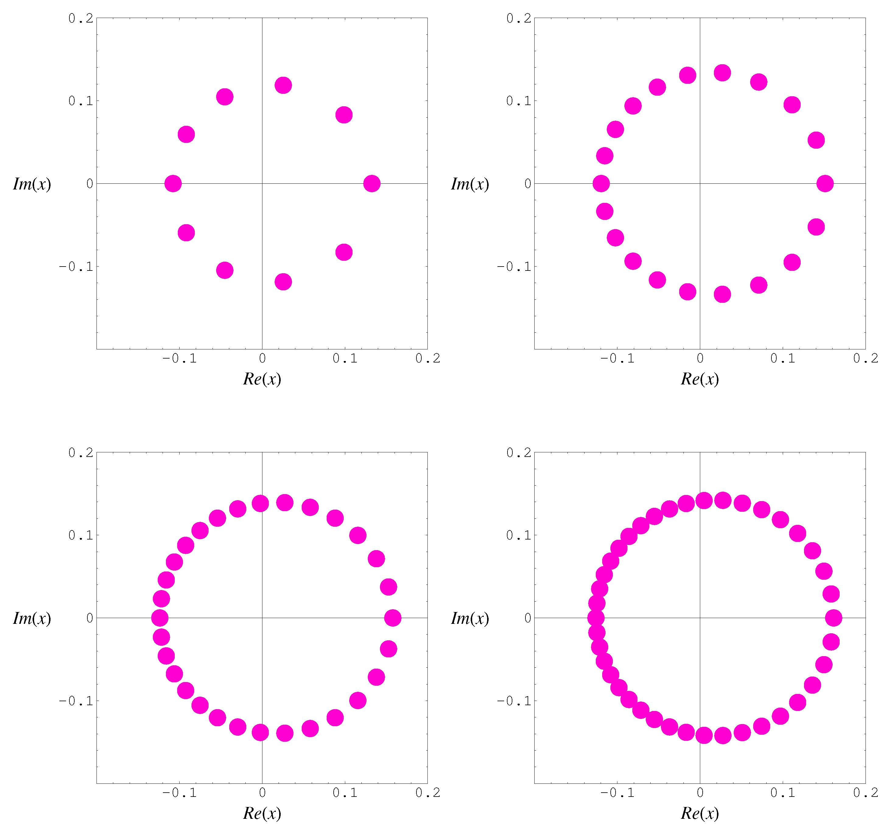
The use of computer has made it possible to identify the zeros of the Carlitz-type $(p,q)$-tangent polynomials $T_{n,p,q}\left(x\right)$. The zeros of the Carlitz-type $(p,q)$-tangent polynomials $T_{n,p,q}\left(x\right)$ for $x\in \mathbb{C}$ are plotted in Figure 1.

In Figure 1(top-left), we choose $n=10,p=1/2$ and $q=1/10$. In Figure 1(top-right), we choose $n=20,p=1/2$ and $q=1/10$. In Figure 1(bottom-left), we choose $n=30,p=1/2$ and $q=1/10$. In Figure 1(bottom-right), we choose $n=40,p=1/2$ and $q=1/10$. It is amazing that the structure of the real roots of the Carlitz-type $(p,q)$-tangent polynomials $T_{n,p,q}\left(x\right)$ is regular. Thus, theoretical prediction on the regular structure of the real roots of the Carlitz-type $(p,q)$-tangent polynomials $T_{n,p,q}\left(x\right)$ is await for further study (Table 1). Next, we have obtained the numerical solution satisfying Carlitz-type $(p,q)$-tangent polynomials $T_{n,p,q}\left(x\right)=0$ for $x\in \mathbb{R}$. The numerical solutions are tabulated in Table 2 for a fixed $p=\frac{1}{2}$ and $q=\frac{1}{10}$ and various value of n.

6. Conclusions and Future Developments

This study constructed the Carlitz-type $(p,q)$-tangent numbers and polynomials. We have derived several formulas for the Carlitz-type $(h,q)$-tangent numbers and polynomials. Some interesting symmetric identities for Carlitz-type $(p,q)$-tangent polynomials are also obtained. Moreover, the results of [18] can be derived from ours as special cases when $q=1$. By numerical experiments, we will make a series of the following conjectures:

Conjecture 1.

Prove or disprove that $T_{n,p,q}\left(x\right),x\in \mathbb{C},$ has $Im\left(x\right)=0$ reflection symmetry analytic complex functions. Furthermore, $T_{n,p,q}\left(x\right)$ has $Re\left(x\right)=a$ reflection symmetry for $a\in \mathbb{R}$.

Many more values of n have been checked. It still remains unknown if the conjecture holds or fails for any value n (see Figure 1).

Conjecture 2.

Prove or disprove that $T_{n,p,q}\left(x\right)=0$ has n distinct solutions.

In the notations: $R_{T_{n,p,q}\left(x\right)}$ denotes the number of real zeros of $T_{n,p,q}\left(x\right)$ lying on the real plane $Im\left(x\right)=0$ and $C_{T_{n,p,q}\left(x\right)}$ denotes the number of complex zeros of $T_{n,p,q}\left(x\right)$. Since n is the degree of the polynomial $T_{n,p,q}\left(x\right)$, we get $R_{T_{n,p,q}\left(x\right)}=n-C_{T_{n,p,q}\left(x\right)}$ (see Table 1 and Table 2).

Conjecture 3.

Prove or disprove that

$$R_{T_{n,p,q}\left(x\right)}=\left\{\begin{array}{cc}1,\hfill & if n=\mathit{odd},\hfill \\ 2,\hfill & if n=\mathit{even}.\hfill \end{array}\right.$$

We expect that investigations along these directions will lead to a new approach employing numerical method regarding the research of the Carlitz-type $(p,q)$-tangent polynomials $T_{n,p,q}\left(x\right)$ which appear in applied mathematics, and mathematical physics (see [11,18,19,20]).

References

1. Araci, S.; Duran, U.; Acikgoz, M.; Srivastava, H.M. A certain (p,q)-derivative operato rand associated divided differences. J. Inequal. Appl. 2016, 2016, 301. [Google Scholar] [CrossRef]
2. Andrews, G.E.; Askey, R.; Roy, R. Special Functions. In Encyclopedia of Mathematics and Its Applications 71; Cambridge University Press: Cambridge, UK, 1999. [Google Scholar]
3. Bayad, A. Identities involving values of Bernstein, q-Bernoulli, and q-Euler polynomials. Russ. J. Math. Phys. 2011, 18, 133–143. [Google Scholar] [CrossRef]
4. Carlitz, L. Expansion of q-Bernoulli numbers and polynomials. Duke Math. J. 1958, 25, 355–364. [Google Scholar] [CrossRef]
5. Choi, J.; Anderson, P.J.; Srivastava, H.M. Some q-extensions of the Apostal-Bernoulli and the Apostal-Euler polynomials of order n, and the multiple Hurwiz zeta function. Appl. Math. Comput. 2008, 199, 723–737. [Google Scholar]
6. Dattoli, G.; Migliorati, M.; Srivastava, H.M. Sheffer polynomials, monomiality principle, algebraic methods and the theory of classical polynomials. Math. Comput. Model. 2007, 45, 1033–1041. [Google Scholar] [CrossRef]
7. Duran, U.; Acikgoz, M.; Araci, S. On (p,q)-Bernoulli, (p,q)-Euler and (p,q)-Genocchi polynomials. J. Comput. Theor. Nanosci. 2016, 13, 7833–7846. [Google Scholar] [CrossRef]
8. Kupershmidt, B.A. Reflection symmetries of q-Bernoulli polynomials. J. Nonlinear Math. Phys. 2005, 12, 412–422. [Google Scholar] [CrossRef]
9. Kurt, V. A further symmetric relation on the analogue of the Apostol-Bernoulli and the analogue of the Apostol-Genocchi polynomials. Appl. Math. Sci. 2009, 3, 53–56. [Google Scholar]
10. He, Y. Symmetric identities for Carlitz’s q-Bernoulli numbers and polynomials. Adv. Differ. Equ. 2013, 246. [Google Scholar] [CrossRef]
11. Ryoo, C.S.; Agarwal, R.P. Some identities involving q-poly-tangent numbers and polynomials and distribution of their zeros. Adv. Differ. Equ. 2017, 213. [Google Scholar] [CrossRef]
12. Shin, H.; Zeng, J. The q-tangent and q-secant numbers via continued fractions. Eur. J. Comb. 2010, 31, 1689–1705. [Google Scholar] [CrossRef]
13. Simsek, Y. Twisted (h,q)-Bernoulli numbers and polynomials related to twisted (h,q)-zeta function and L-function. J. Math. Anal. Appl. 2006, 324, 790–804. [Google Scholar] [CrossRef]
14. Srivastava, H.M. Some generalizations and basic (or q-) extensions of the Bernoulli, Euler and Genocchi Polynomials. Appl. Math. Inform. Sci. 2011, 5, 390–444. [Google Scholar]
15. Srivastava, H.M.; Pintér, Á. Remarks on some relationships between the Bernoulli and Euler polynomials. Appl. Math. Lett. 2004, 17, 375–380. [Google Scholar] [CrossRef]
16. Srivastava, H.M.; Pintér, Á. Addition theorems for the Appell polynomials and the associated classes of polynomial expansions. Aequ. Math. 2013, 85, 483–495. [Google Scholar]
17. Choi, J.; Anderson, P.J.; Srivastava, H.M. Carlitz’s q-Bernoulli and q-Euler numbers and polynomials and a class of generalized q-Hurwiz zeta functions. Appl. Math. Comput. 2009, 215, 1185–1208. [Google Scholar]
18. Hwang, K.W.; Ryoo, C.S. On Carlitz-type q-tangent numbers and polynomials and computation of their zeros. J. App. Math. Inform. 2017, 35, 495–504. [Google Scholar] [CrossRef]
19. Ryoo, C.S. A note on the tangent numbers and polynomials. Adv. Stud. Theor. Phys. 2013, 7, 447–454. [Google Scholar] [CrossRef]
20. Agarwal, R.P.; Kang, J.Y.; Ryoo, C.S. Some properties of (p,q)-tangent polynomials. J. Comput. Anal. Appl. 2018, 24, 1439–1454. [Google Scholar]
Figure 1. Zeros of T n , p , q ( x ) .
Symmetry 10 00395 g001