Barycenter Theorem in Phase Characteristics of Symmetric and Asymmetric Windows

Abstract

Asymmetric windows are of increasing interest to researchers because of the nonlinear and adjustable phase response, as well as alterable time delay. Short-time phase distortion can provide an essential improvement in speech coding, and also has better performance in speech recognition. The merits of asymmetric windows in the aspect of spectral behaviors have an important function in frequency component detection and parameter estimation. In this paper, the phase response of windows were further studied, and the phase characteristics of symmetric and asymmetric windows are described. The relationship between the barycenter of windows in the time domain, and the phase characteristic at the center of the main lobe in the frequency domain, was established. In light of the relationship, an improved version of the asymmetric window- based frequency estimation algorithm was proposed. The improved algorithm has advantages of straightforward implementation and computational efficiency. The numeric simulation results also indicate that the improved approach is more robust than the traditional method against additive random noise.

1. Introduction

Windows are a kind of weighting function that are introduced to reduce the spectral leakage in spectrum analysis [1]. Classic windows have constant time delay and linear phase response due to the symmetry and time shifting causality-imposed in the time domain [2]. In recent years, asymmetric windows have attracted increasing concerns due to the nonlinear and adjustable phase response, as well as alterable time delay [2]. Short-time phase distortion can lead to better recognition in speech processing and bring a lot of advantages in speech coding [3,4,5,6,7]. These asymmetric windows with extended discrimination capacity are very good candidates for the detection of closely spaced frequency components [8]. The characteristics of the adjustable spectral phase in asymmetric windows also play an important role in parameter estimation [9]. However, it should be pointed out that most of the past literature, so far, has been mainly focused on the construction of asymmetric windows or the amplitude response [2,3,4]. Although the alterable phase response of asymmetric windows is of great benefit to scientific fields or engineering applications, such as speech recognition and parameter estimation, there have been relatively few studies devoted to the theoretical analysis of phase response.

For example, when asymmetric windows are applied in phase difference-based frequency estimation implemented by discrete Fourier Transform (DFT), an accurate frequency estimate can be obtained through only one sample frame [9]. The critical point is to find the abscissa where the phase difference is zero, because the intersection of the phase lines of a symmetric window and its corresponding asymmetric window is always at the center of the main lobe [9]. Since it is difficult to find an analytical solution, it becomes a numeric root-finding problem. In [9], the secant method was suggested to approximate the normalized theoretical frequency. However, it is required to compute additional Fourier coefficients in each iteration, where intensive computational effort is involved and, thus, poses a heavy burden on the overall cost of the algorithm. This problem extremely weakens the application of the estimation algorithm in the presence of noise, especially in the situation where real-time computation is demanded. If the slope of the secant lines can be computed steadily in advance, the amount of calculation can be sharply decreased because of fast convergence. For a symmetric window, the phase response can be easily worked out, while, for an asymmetric window, it is difficult due to the nonlinearity and alterability. In this paper, our aim was to study the phase characteristics of asymmetric windows and deduce the inner relationship between samples of window in the time domain and its slope of the phase response in the frequency domain.

This paper is organized as follows. In Section 2, the phase response of symmetric windows, in the form of continuous time, is explored, and the DFT-even window and true-even window in the form of discrete time are discussed. In Section 3, the phase characteristics of asymmetric windows are studied, and the relationship between the barycenter of windows and the phase characteristic is established. In Section 4, an improved version of the phase difference-based frequency estimation algorithm is proposed by taking advantage of the phase characteristic of asymmetric windows. A numerical comparison study between the improved approach and the traditional approach is also performed in this section. In Section 5, the main conclusions are summarized.

2. Phase Response of Symmetric Windows

2.1. Phase Response of Symmetric Windows

Considering a window function $w(t)=w(-t)$, the time interval of $w(t)$ is T. The Fourier transform of the window can be expressed as [10]

$$F(f)={\displaystyle \underset{-\infty }{\overset{+\infty }{\int }}w(t)e^{-j2\pi ft}dt}={\displaystyle \underset{-T/2}{\overset{T/2}{\int }}w(t)e^{-j2\pi ft}dt}$$

(1)

Since $w(t)$ is even and real, $F(f)$ is a real even function. Obviously, the phase is 0 or $\pi$, depending on the sign of $F(f)$. If a time shift on the window function $w(t)$ is T/2, the Fourier transform of the time-shifted window function $\widehat{w}(t)=w(t+T/2)$ would be [11]

$$\widehat{F}(f)=F(f)e^{-j\pi fT}$$

(2)

Accordingly, the phase is

$$\varphi (f)=-\pi fT$$

(3)

It is indicated that a time shift on a window function would introduce a linear phase shift.

2.2. Phase Response of Sampled Symmetric Windows

As a symmetric window in the form of continuous time is an even function about the origin, the discrete window with an odd number of points N is also presented as symmetrical. The overall points include (N − 1)/2 points on each side, and a peak point in the middle of the window. For an even number of points, a discrete window is obtained after the right endpoint is discarded. This is DFT-even, referred to in [1]. In that paper, Harris also mentioned that the window with the absolute even symmetry, rather than that with the implied symmetry with the missing endpoint, was designed by much of the literature and incorporated in many software libraries [1]. However, whether all the DFT-even windows have a strictly linear phase is still unknown, and so far, the differences and relationships between the phase of DFT-even windows and that of absolute-even windows have not been analyzed. To answer these questions, a new and uniform perspective of the process from a continuous symmetric window to a discrete window will be presented in the latter part of this section. We used the triangle window as an example. The triangle window in the form of continuous time can be written as

$$w(t)=\{\begin{array}{cc}1-2\left|t\right|/T,& \left|t\right|\le T/2,\hfill \\ 0,& \mathrm{else}.\hfill \end{array}$$

(4)

the period of which is T. The interval can be separated into N slices by N + 1 points. A discrete window with an odd or even number of points can be obtained by keeping or removing the last point. This is the routine operation. Now, we consider a sampling train $q(t)$, which can be shifted by a coefficient $\varsigma$. It is described as

$$q(t)={\displaystyle \sum _{n=-\infty }^{+\infty }\delta (t-n\Delta T-\varsigma )},$$

(5)

where $\Delta T$ is sample interval; and $\varsigma$ is the shifting factor between zero and $\Delta T$. By making $\Delta T$ equal to $T/N$ and $\epsilon$ equal to $\varsigma /\Delta T$, a discrete triangle window sampled from the continuous one with $N$ points is obtained. Given the radix-2 operations were implemented in fast Fourier Transform (FFT), we only discuss the discrete window with an even number of points in detail. The discrete triangle window can be described as

$$w(n)=1-2|n+\epsilon |/N,$$

(6)

where $0\le \epsilon <1,n=-N/2,-N/2+1,\cdots \cdots ,N/2-2,N/2-1$. The value of each point in the discrete triangle window is dependent upon the parameter $\epsilon$. In this paper, special cases with $\epsilon =0$ and $\epsilon =0.5$ were considered. When $\epsilon =0$, it is exactly the same as the DFT-even window. When $\epsilon =0.5$, the window is absolutely symmetric. Two cases of a triangle window with 32 samples are shown in Figure 1.

Figure 1. (a) DFT-even triangle window; (b) True-even triangle window.

In the two cases, the results of DFT were all real, because of the symmetry and real in the time domain. As a result, after the windows were shifted, both of them had a linear phase, with the difference being that the slope for the DFT-even window was $-\pi$ (see Appendix A) and the slope for the true-even window was $-(N-1)\pi /N$ (see Appendix B). This is because the number of shifting points was N/2 for the DFT-even window and was (N − 1)/2 for the true-even window. Figure 2, Figure 3 and Figure 4 show the normalized log-magnitude response (NLMR), the normalized phase response (NPR), and the derivative of normalized phase response (DNPR). The results coincided well with the theoretical analysis.

Figure 2. Normalized log-magnitude response of triangle window.

Figure 3. Normalized phase response of triangle window.

Figure 4. Derivative of normalized phase of triangle window.

When it comes to windows with non-zero endpoints, things get more complex. For example, the Hamming window can be written as

$$f(t)=\{\begin{array}{cc}q+(1-q){\cos }^2(\pi t/T),& \left|t\right|\le T/2,\hfill \\ 0,& \mathrm{else}.\hfill \end{array}$$

(7)

When $\epsilon$ = 0.5, the phase slope for the true-even window is still $-(N-1)\pi /N$. However, when $\epsilon$ = 0, the DFT-even window has a nonlinear, but approximately linear phase, due to loss of symmetry in the time domain. For an enough large N, the slope of the phase gets close to $-\pi$. For the two cases of Hamming window with 32 samples, the normalized log-magnitude response, the normalized phase response, and the derivative of normalized phase are shown in Figure 5, Figure 6, Figure 7 and Figure 8, respectively. It is clear that all absolute-even ($\epsilon$ = 0.5) windows have a strictly linear phase. The phase for some DFT-even ($\epsilon$ = 0) windows are strictly linear, and some are not, which is decided by the value of the endpoint.

Figure 5. (a) DFT-even Hamming window; (b) True-even Hamming window.

Figure 6. Normalized log-magnitude response of Hamming window.

Figure 7. Normalized phase response of Hamming window.

Figure 8. Derivative of normalized phase of Hamming window.

3. Phase Response of Asymmetric Windows

3.1. Phase Response of Asymmetric Windows

For a symmetric window, the symmetric center is the peak point. The slope of phase is determined by the causality-imposed time shift. Since all symmetric windows have a constant time delay T/2, they have the same phase response [2]. Before further discussion, we introduced an indicator, $\overline{\tau }$, called the normalized time delay factor (NTDF), to evaluate the time delay of different lengths of windows. This is defined as the time delay $\tau$ of a window scaled by the interval that the window covers.

$$\overline{\tau }=\frac{\tau }{T}.$$

(8)

Obviously, we have $0<\overline{\tau }<1$ and the NTDF of all symmetric windows is 1/2. For an asymmetric window, we would also like to find the NTDF. If we denote $\varphi (f)$ as the phase response of a time-shifting asymmetric window $\widehat{w}\left(t\right)$, according to the Taylor series expansion, one can have

$$\varphi (f)=\varphi (f_0)+{\varphi }^{\prime }(f_0)(f-f_0)+o(f-f_0).$$

(9)

The phase response in the main lobe, and especially the phase response near the main lobe center is of more significance, as it has a decisive influence on the phase distortion of the tapered signal [11,12,13]. The problem is more notable for the FFT of a discrete time signal, due to the picket fence effect [13,14]. The phase distortion is determined by the frequency deviation and the variation of phase response near the main lobe center of the adopted window [9]. As a result, expanding $\varphi (f)$ around the center in the main lobe with $f_0=0$, one can reach

$$\varphi (f)=\varphi (0)+{\varphi }^{\prime }(0)f+o(f).$$

(10)

Since the weighting function is real, $\varphi (0)=0$. Equation (10) can be simplified as

$$\varphi (f)={\varphi }^{\prime }(0)f+o(f).$$

(11)

Equation (11) indicates that the phase near the center of the main lobe can be approximated by two parts: the linear part ${\varphi }^{\prime }(0)f$ and the higher order part. According to a similar concept used in symmetric windows, we introduced the general time delay (GTD) in asymmetric windows. Assuming $\tau$ denotes the general time delay, and considering the relationship between time delay and the linear part of phase, we have

$$\varphi (f)\cong {\varphi }^{\prime }(0)f=-2\pi f\tau .$$

(12)

The GTD of an asymmetric window can be computed by

$$\tau =-\frac{{\varphi }^{\prime }(0)}{2\pi }.$$

(13)

Considering the substitution ${\varphi }^{\prime }(0)=-2\pi Bary[\widehat{w}(t)]$ (See Appendix C), the GTD can be finally expressed as

$$\tau =Bary[\widehat{w}(t)].$$

(14)

Equation (14) indicates that the general time delay is solely determined by the barycenter of the weighting factors and that window function can be adjusted in the time domain to change the time delay. Specifically, the time delay of all symmetric windows is T/2, as the barycenter is located at the symmetric center. Equation (14) not only gives a mathematical analysis of the time delay, but also implies that the phase characteristics around the center of the main lobe can be quantitatively adjusted. According to Appendix C, the derivative of the phase in the main lobe center can be computed by

$${\varphi }^{\prime }(0)=-2\pi Bary[\widehat{w}(t)].$$

(15)

3.2. Phase Response of Sampled Asymmetric Windows

Similar to the asymmetric windows in the form of continuous time, the discrete time asymmetric windows have the same property. If $\mu$ denotes the general time delay, for the asymmetric windows $\widehat{w}(n)$, the derivative of the phase at the center of the main lobe (DPCM) ${\phi }^{\prime }(0)$ can be calculated by

$${\phi }^{\prime }(0)=-2\pi \overline{\mu },$$

(16)

where $\overline{\mu }=\mu /N$ denotes the normalized GTD. According to the conclusion in Appendix D, the normalized GTD can be finally expressed as

$$\overline{\mu }=Bary[\widehat{w}(n)]/N.$$

(17)

It should be pointed out that for an asymmetric window, the asymmetry due to the discrete sampling discussed in Section 2.2 is much less critical when compared with the asymmetry of itself, and Equation (16) is valid for all sampling cases.

4. Applications and Numerical Simulations

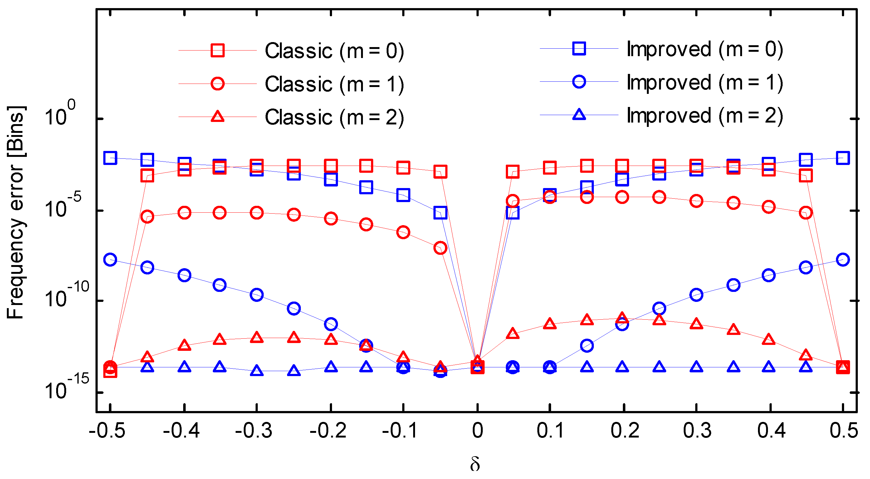
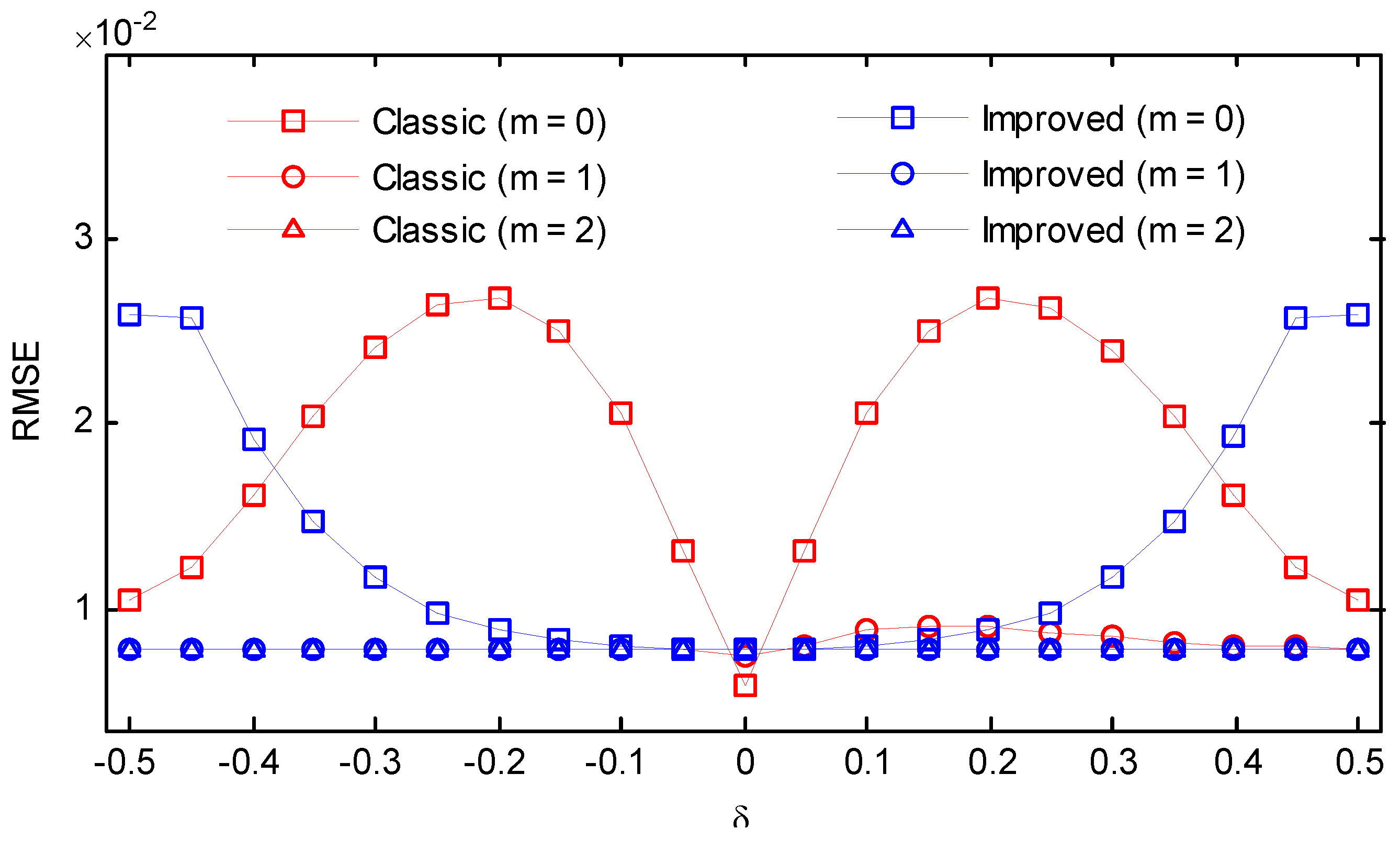
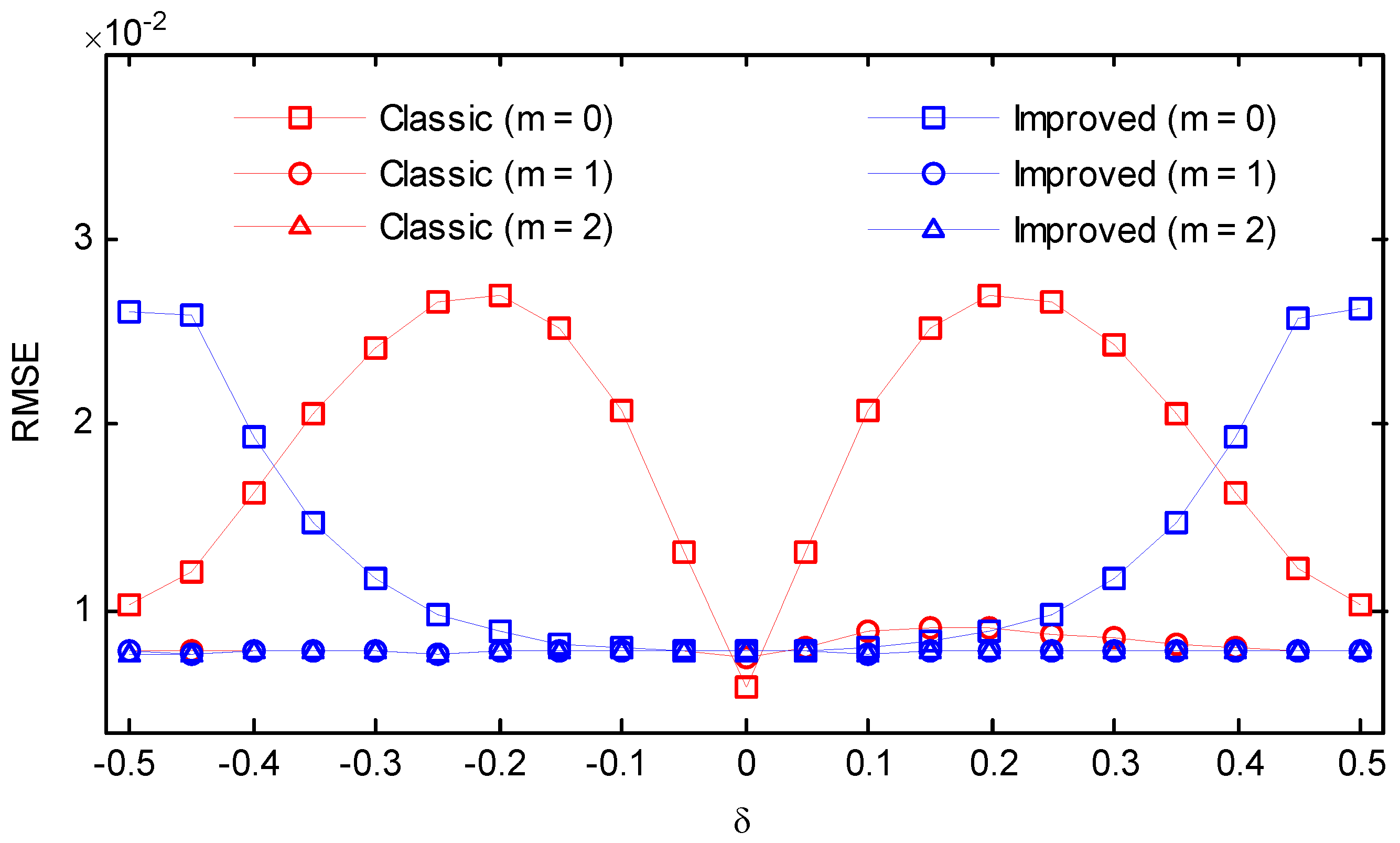
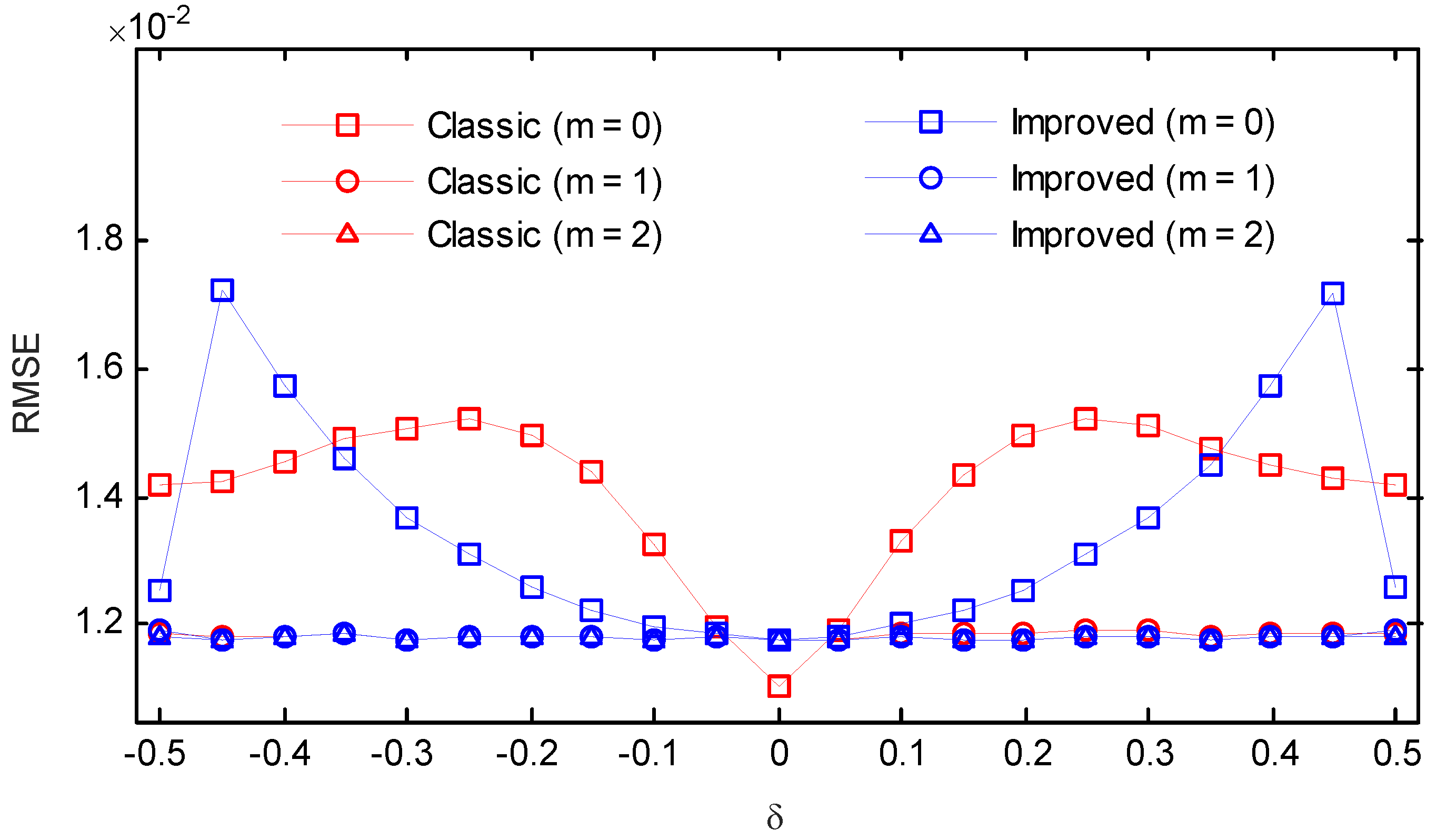
4.1. Application in Frequency Estimation

It has been demonstrated that if asymmetric windows are introduced in frequency estimation, some inherent defects in the traditional parameter estimation algorithms can be overcome [9]. For example, by replacing symmetric windows with proper asymmetric windows, frequency estimation can be achieved by only one segment of samples, rather than two segments in the traditional phase difference-based algorithms, thus yielding better performance in the estimation of closely spaced frequency components [9]. Furthermore, the resistance of traditional algorithms against additive noise can be improved with the proper selection of asymmetric windows. However, it should also be stressed that the improvement is at the expense of a remarkable increase in computational burden as the simple relationship between the normalized frequency deviation and the phase difference disappears, due to the nonlinear phase of asymmetric windows. The calculation of estimate becomes a root-finding problem, and the secant method was suggested in [9] to avoid the computation of a derivative in Newton’s method. The secant method is defined by the recurrence relation

$$k_m=k_{m-1}+\Delta \zeta (k_{m-1})\frac{k_{m-1}-k_{m-2}}{\Delta \zeta (k_{m-1})-\Delta \zeta (k_{m-2})}=k_{m-1}+\Delta \zeta (k_{m-1})/{\eta }_{m-1},$$

(18)

where $k_m$ denotes the normalized frequency estimate in each iteration; $\Delta \zeta (k_m)$ denotes the phase difference at frequency $k_m$; and ${\eta }_m$ is defined as

$${\eta }_m=\frac{\Delta \zeta (k_m)-\Delta \zeta (k_{m-1})}{k_m-k_{m-1}}.$$

(19)

It should be pointed out that we have the relationship that

$$\underset{m\to \infty }{\lim }{\eta }_m=\underset{m\to \infty }{\lim }\frac{\Delta \zeta (k_m)-\Delta \zeta (k_{m-1})}{k_m-k_{m-1}}=\Delta {\phi }^{\prime }(0),$$

(20)

where $\Delta {\phi }^{\prime }(0)={\phi }_1^{\prime }(0)-{\phi }_2^{\prime }(0)$, ${\phi }_1^{\prime }(\cdot )$ and ${\phi }_2^{\prime }(\cdot )$ are the DPCM of the two adopted windows, respectively. Moreover, ${\phi }_1^{\prime }(f)$ and ${\phi }_2^{\prime }(f)$ vary slightly around the center in the main lobe and the frequency estimate returned by coarse search is also near the center of the modulated main lobe. Accordingly, we can rewrite the recurrence relation by replacing ${\eta }_m$ with $\Delta {\phi }^{\prime }(0)$.

$$k_m=k_{m-1}+\Delta \zeta (k_{m-1})/\Delta {\phi }^{\prime }(0)$$

(21)

Equation (21) avoids the calculation of the finite difference ${\eta }_m$. While, in Equation (18) ${\eta }_m$ is required to be computed in each iteration and more importantly, ${\eta }_m$ may become unstable once intensive random noise is involved. In contrast, $\Delta {\phi }^{\prime }(0)$ is only dependent on the adopted windows and is, consequently, a constant value in each iteration. The frequency components and random noise have no influence on $\Delta {\phi }^{\prime }(0)$, and thus $\Delta {\phi }^{\prime }(0)$ can be computed in advance once the window is determined. As a result, Equation (21) becomes more robust and more efficient than Equation (18) in the presence of interference or random noise. In addition, the requirement of memory for the implementation of Equation (21) is also less than that of Equation (18). All those features make it well suited for application in practice engineering. Finally, the improved estimation algorithm can be summarized as follows:

(1)

Obtain the first discrete-time signal $y(n)=x(n)w(n)$, where $x(n)$ is the raw sequence with N samples and $w(n)$ is a symmetric window.

(2)

Obtain the second sequence $\widehat{y}(n)=x(n)\widehat{w}(n)$, where $\widehat{w}(n)$ is the corresponding asymmetric window.

(3)

Perform a coarse search on $|Y(k)|$, where $Y(\cdot )$ is FFT of $y(n)$, to determine the bin number l with the largest magnitude.

(4)

Calculate the window-related coefficient $\Delta {\phi }^{\prime }(0)$ as well as the phase difference between the two sequences $\Delta \zeta (l)=\arg [Y(l)]-\arg [\widehat{Y}(l)]$, where $\widehat{Y}(l)$ is the DFT coefficient of $\widehat{y}(n)$.

(5)

Return the coarse estimate $k_0=l+\Delta \zeta (l)/\Delta {\phi }^{\prime }(0)$.

(6)

Obtain the further refined estimate by the iterations $k_m=k_{m-1}+\Delta \zeta (k_{m-1})/\Delta {\phi }^{\prime }(0)$.

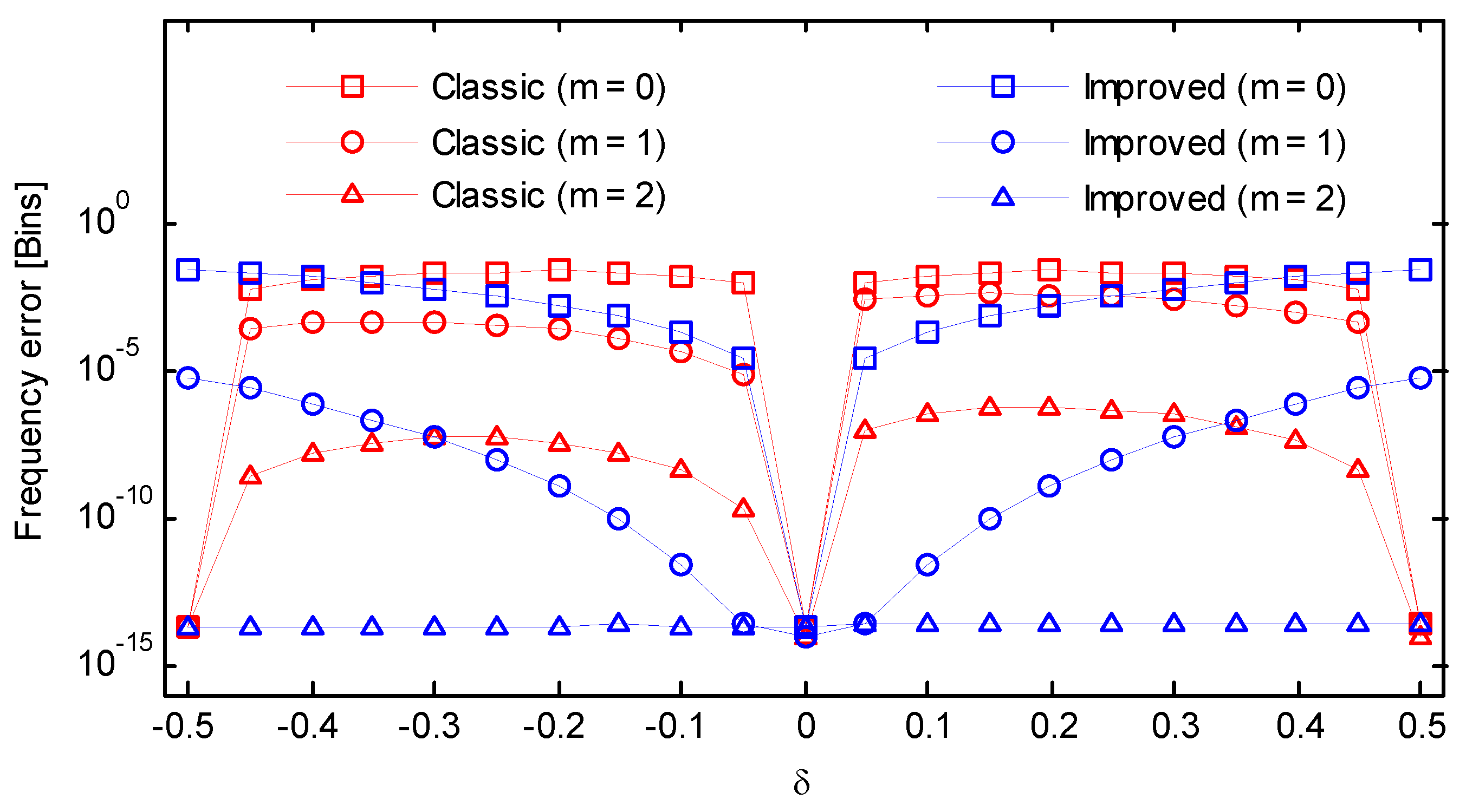
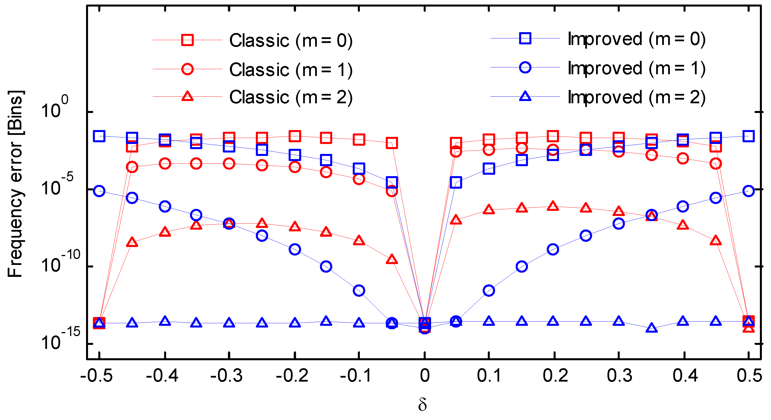
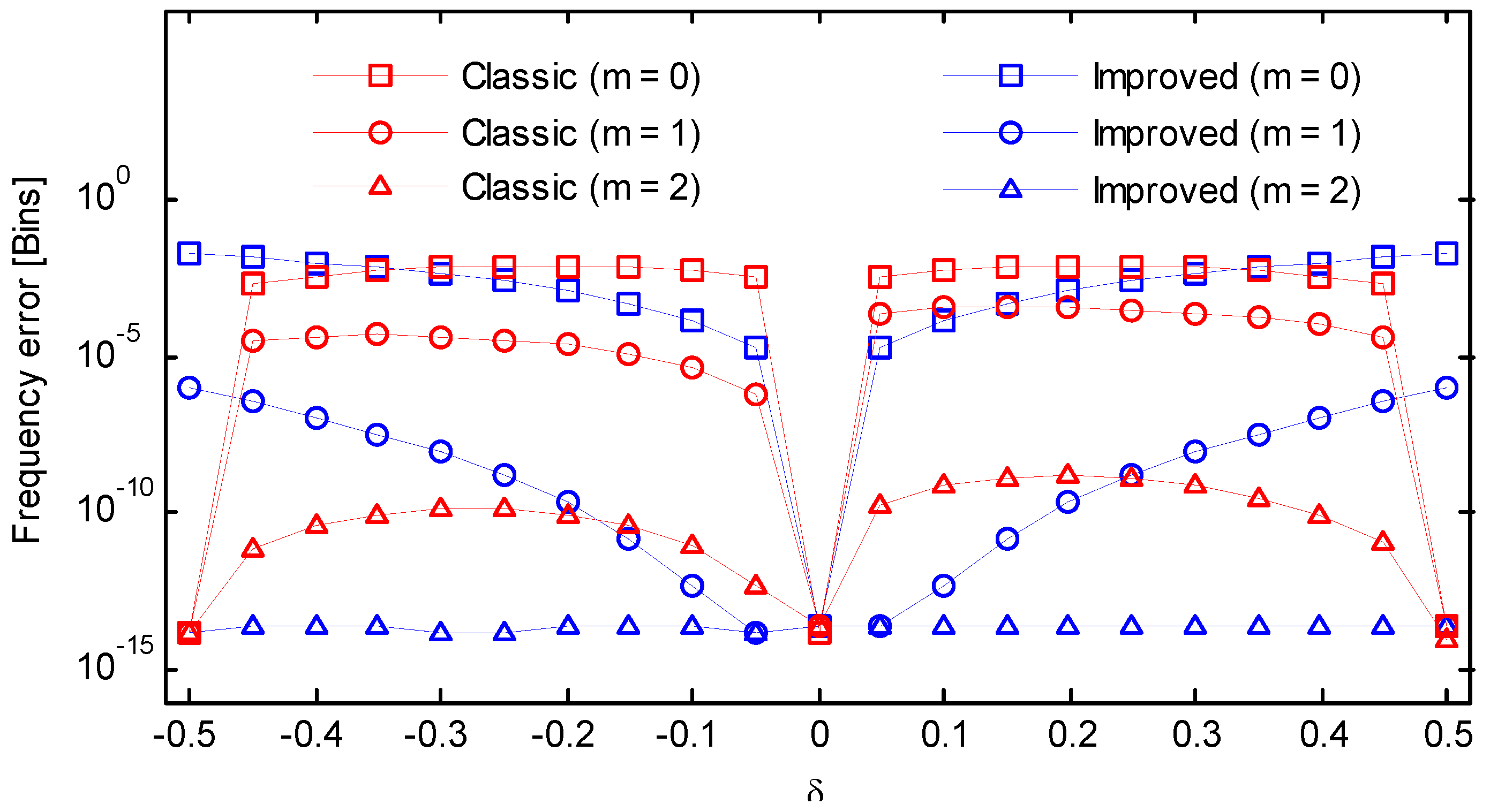
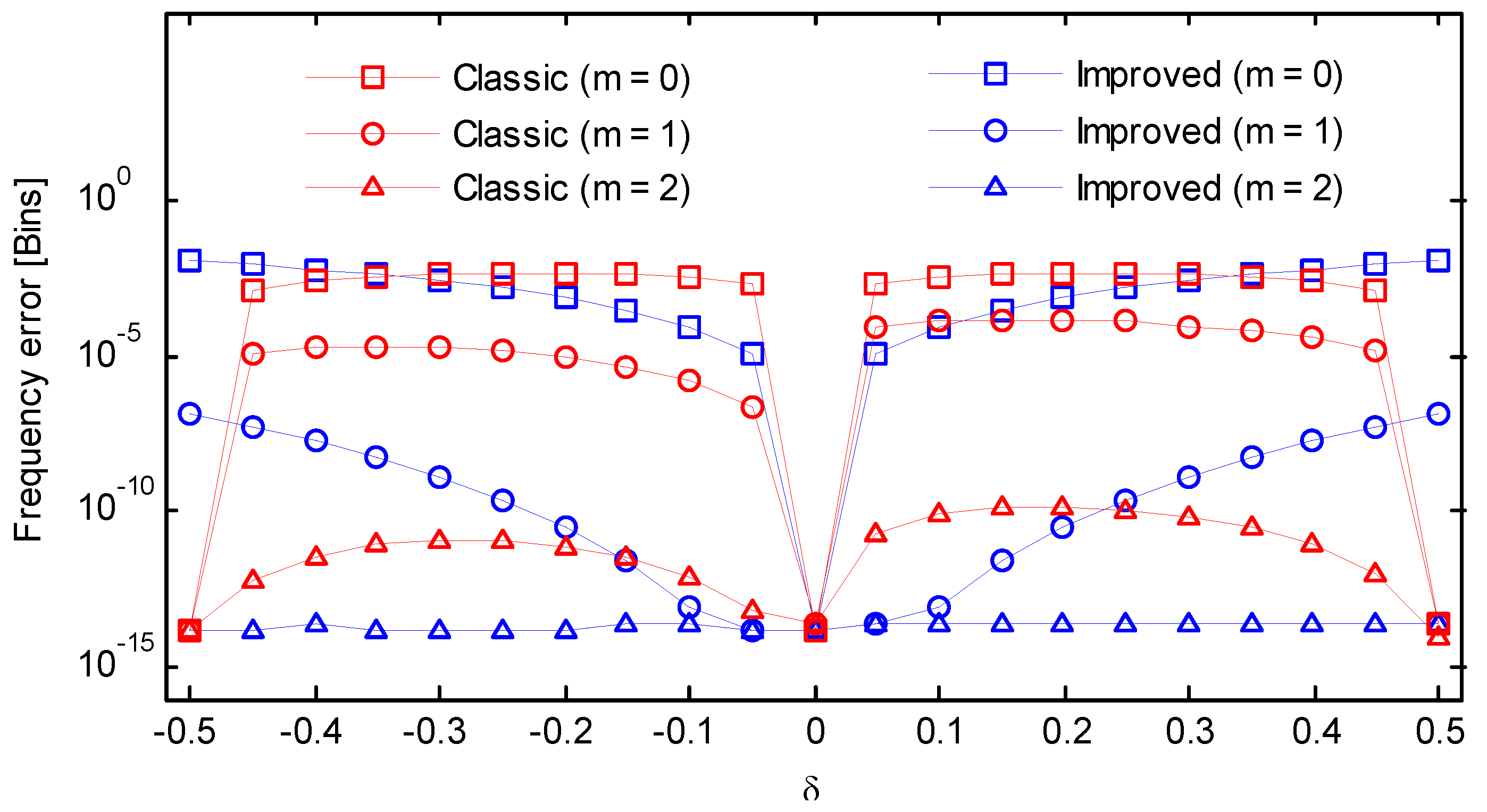
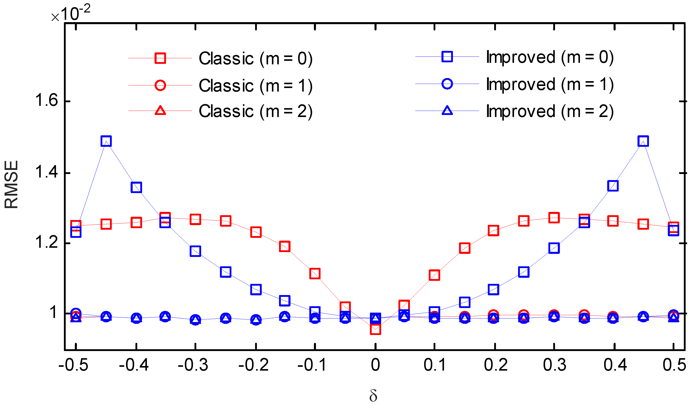
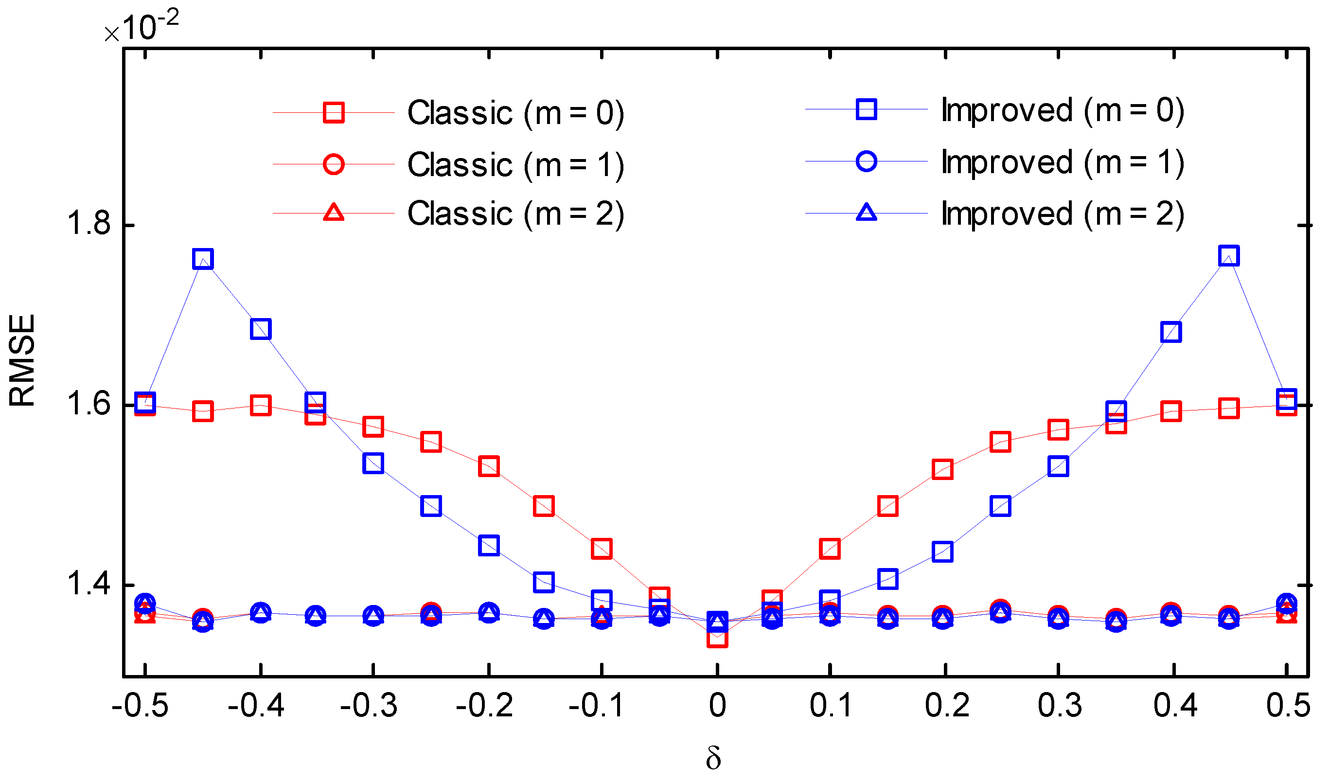
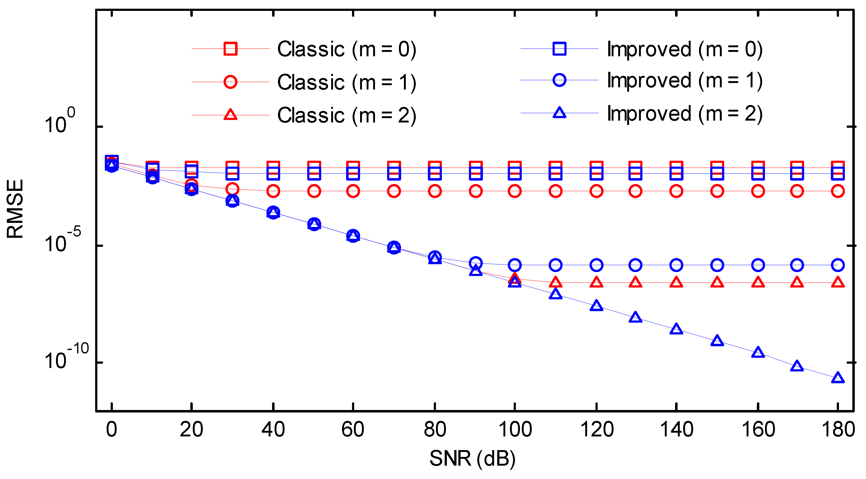
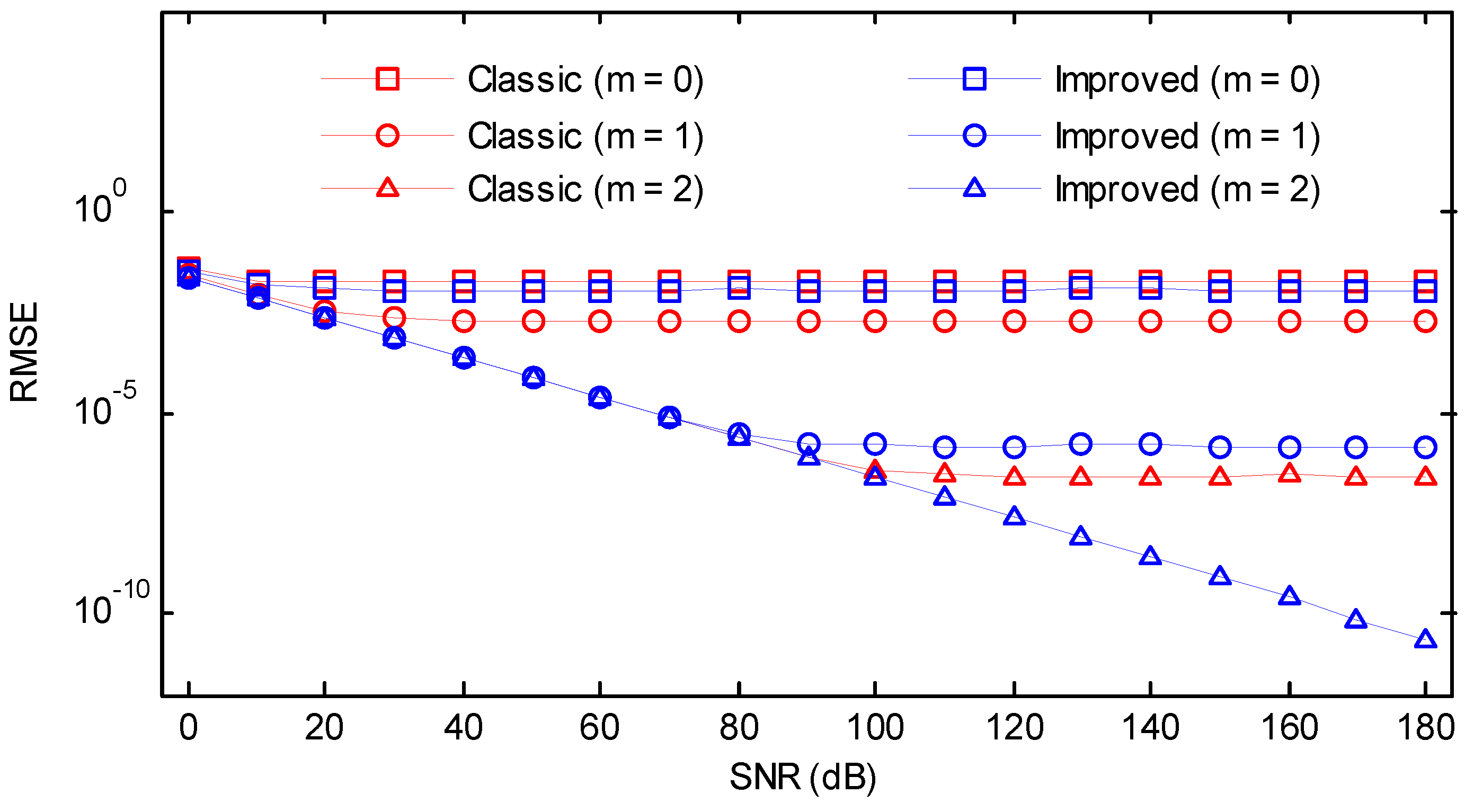
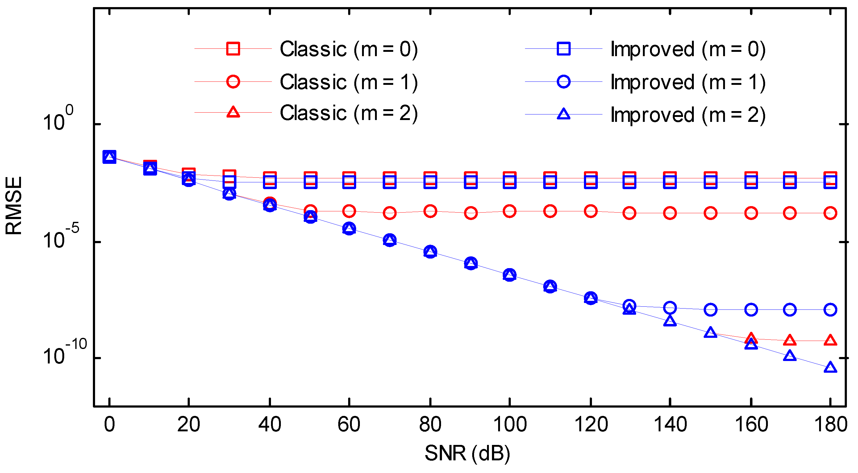
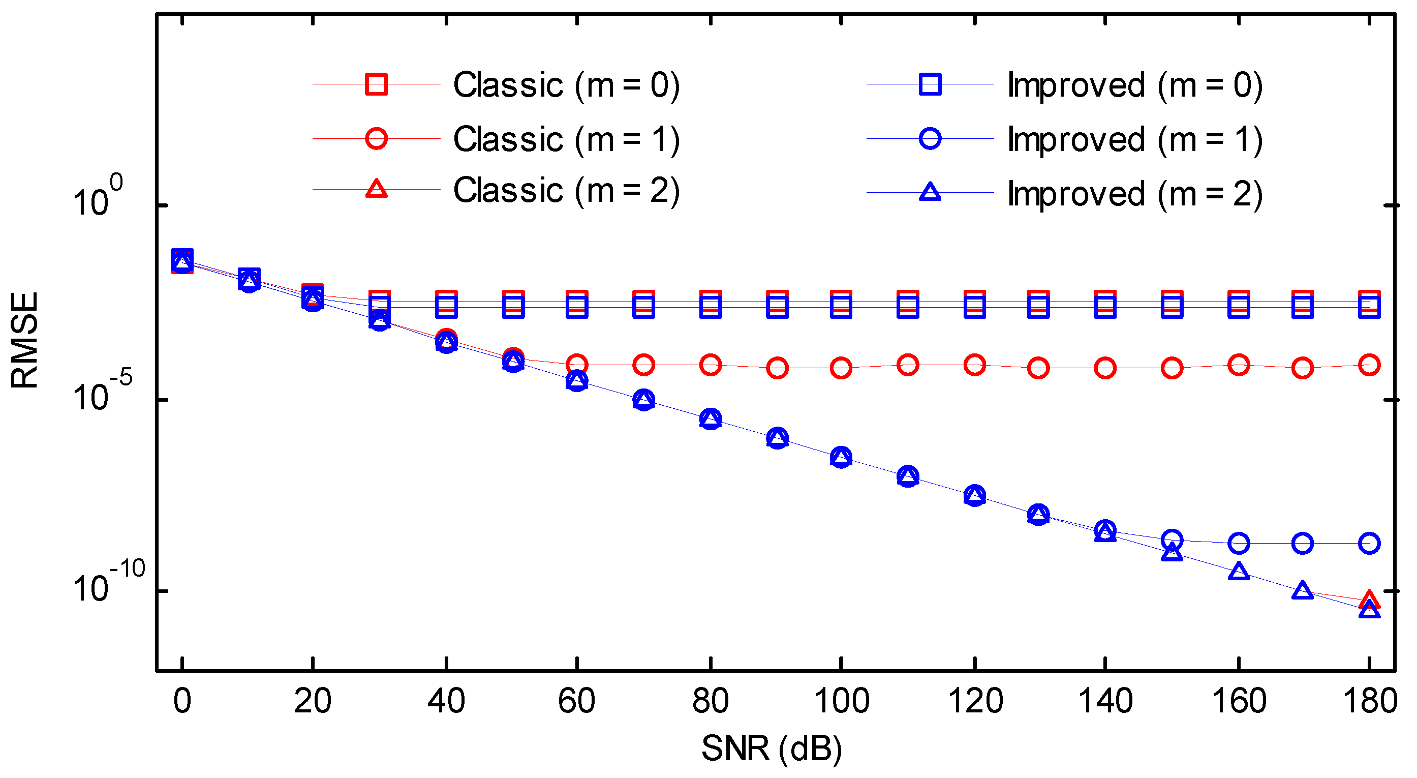
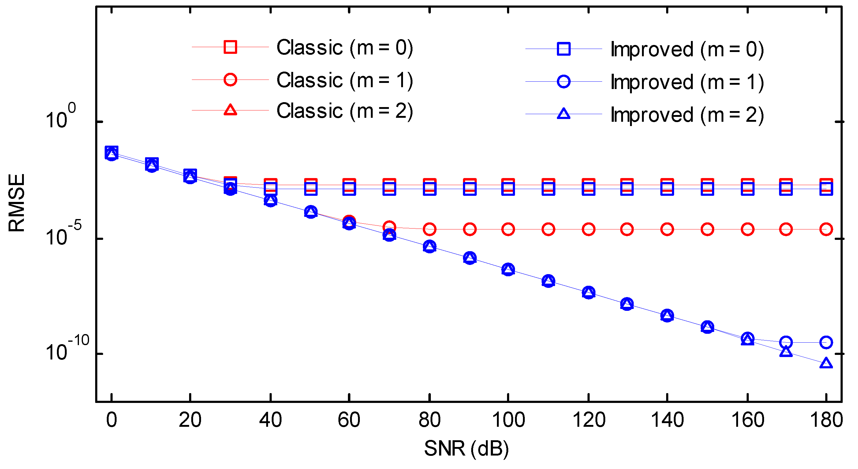
4.2. Simulation and Results

In order to evaluate the effectiveness of Equation (21) as well as compare it with the traditional algorithm, some simulations were designed. For simplicity but without loss of generality, a single discrete complex exponential was considered, which can be generated according to Equation (22).

$$x(n)=A_0{e}^{j(2\pi n{f}_0/f_s+\theta )},n=0,1,2,3\dots \dots N-1$$

(22)

In Equation (22), the amplitude $A_0$ was set to 1. Both the sampling rate $f_s$ and the number of analyzed samples N was set to 256, resulting in a frequency resolution of $\Delta f=f_s/N=1$. First, we considered the cases free of noise. The frequency scanned from 63.5 to 64.5 in steps of 0.05. For each frequency, the phase scanned from $-\pi$ to $\pi$ in steps of $\pi /72$, and the maximum absolute estimation error between the estimate and the theoretical value was selected as the result. All frequency estimates were scaled by frequency resolution and expressed in frequency bin. The adopted asymmetric windows were [t]₂-windows defined in [2], which was constructed by the truncation method. The remaining errors for the Kaiser–Bessel window, Gaussian window, Hanning window, Hamming window, and Blackman window were reported in Figure 9, Figure 10, Figure 11, Figure 12 and Figure 13 as a function of frequency deviation. As can be seen from these figures, the asymmetric windows-based phase difference method had good compatibility with different window functions. The maximum absolute estimation errors for the classic method with m = 0 were about 10⁻³~10⁻². By performing an iteration, the level decreased to 10⁻⁵~10⁻⁴. Without iteration, the improved method had a similar performance to the classic method but attained a worst case at $\delta =0.5$. However, after an iteration, the errors sharply decreased and were all below 10⁻⁵. The remaining errors could be completely removed after two iterative operations even for the case where $\delta =0.5$. As a result, in the absence of noise, an iteration in the proposed algorithm was enough to achieve a high accurate result.

Figure 9. Frequency errors of the classic and the improved secant method (Kaiser–Bessel window, $\beta =0.5$).

Figure 10. Frequency errors of the classic and the improved secant method (Gaussian window, $\alpha =1$).

Figure 11. Frequency errors of the classic and the improved secant method (Hanning window).

Figure 12. Frequency errors of the classic and the improved secant method (Hamming window).

Figure 13. Frequency errors of the classic and the improved secant method (Blackman window).

Now, we considered that Equation (22) was contaminated with an additive Gaussian random noise z(n). The parameter settings were the same as Figure 9, Figure 10, Figure 11, Figure 12 and Figure 13, except that the phase was randomly selected. The variance of additive white Gaussian noise ${\sigma }^2$ was set to $A_0^2/10$, indicating signal-to-noise ratio (SNR) equal to 10 dB. SNR expressed in dB was defined as

$$SN{R}_{dB}=10{\log }_{10}{A}_0^2/{\sigma }^2.$$

(23)

An amount of 100,000 instances of such test signals were generated for each frequency, and the root-mean-square error (RMSE) was evaluated. The simulation results for the five considered windows are shown in Figure 14, Figure 15, Figure 16, Figure 17 and Figure 18. For m = 0, the classic secant method had good performance in the vicinity of $\delta =0$, however, it showed a much worse performance in the rest of the cases. After an iteration, the RMSEs of the classic secant method declined notably, but the fluctuation could be still observed. If m = 2, the values can be maintained at the same level for the whole range of frequency deviation. In contrast, the improved secant method had a more rapid convergence and the errors stayed steady for different frequency deviations after only one iteration. The proposed approach did not seem to capture a substantial improvement by performing another iteration after the first iteration. The benefit from more iterations was limited, but each iteration required a calculation of two DFT coefficients, which would increase the overall computational effort. Hence, it can be concluded that if a moderate noise is involved, performing one iteration after the coarse compensation in step (5) is enough for the improved secant method, as the errors due to different frequency deviation can be eliminated.

Figure 14. RMSEs of the classic and the improved secant method (SNR = 10 dB, Kaiser–Bessel window, $\beta =0.5$).

Figure 15. RMSEs of the classic and the improved secant method (SNR = 10 dB, Gaussian window, $\alpha =1$).

Figure 16. RMSEs of the classic and the improved secant method (SNR = 10 dB, Hanning window).

Figure 17. RMSEs of the classic and the improved secant method (SNR = 10 dB, Hamming window).

Figure 18. RMSEs of the classic and the improved secant method (SNR = 10 dB, Blackman window).

We also investigated the RMSEs of the classic and the improved secant method for a wide range of SNRs from 0 dB to 180 dB with a step of 10 dB. The normalized frequency, as well as the phase, were randomly chosen. The other simulation parameters were kept invariant. As can be seen in Figure 19, Figure 20, Figure 21, Figure 22 and Figure 23, for some conditions, the RMSEs may become flat after certain SNR as the bias becomes the dominant source of error. In the case where enough iterations were performed, the remaining bias could be completely eliminated, and the RMSEs were linear for the entire range of SNR. The figures were very informative regarding the trade-off between the bias and variance for different iterations. Without iterations, the classic method was first saturated at SNR ≈ 10 dB, followed by the improved method. If an iteration was performed, the values for the improved method sharply decreased, and the RMSEs were much smaller and less than 10⁻⁶. However, a high level of RMSEs remained for the classic method. If two iterations were performed, the RMSEs of the improved version would be merely dependent on the random noise, while for the classic method, the bias may still be significant when a high SNR was encountered. In most practical situations, the influence of noise is usually more important than the bias. As a result, one iteration was sufficient for the proposed algorithm to produce satisfactory results even in the presence of noise.

Figure 19. RMSEs of the classic and the improved secant method versus SNR (Kaiser–Bessel window, $\beta =0.5$).

Figure 20. RMSEs of the classic and the improved secant method versus SNR (Gaussian window, $\alpha =1$).

Figure 21. RMSEs of the classic and the improved secant method versus SNR (Hanning window).

Figure 22. RMSEs of the classic and the improved secant method versus SNR (Hamming window).

Figure 23. RMSEs of the classic and the improved secant method versus SNR (Blackman window).

5. Conclusions

In this paper, the phase characteristics of symmetric and asymmetric windows were studied. It was shown that the phase characteristics were closely related to the time delay of the windows. The quantitative relationship between the barycenter of the windows in the time domain and the phase slope at the main lobe center in the frequency domain was derived. On the basis of the relationship, the traditional phase difference method was improved by a simplified secant method. This was illustrated through simulations where the improved algorithm not only had the merits of simple implementation and computational efficiency, but also had the advantage of robustness against additive random noise as the proposed algorithm with only one additional iteration was sufficient to guarantee an accurate estimate even in the presence of noise.

References

- Harris, F.J. On the use of harmonic analysis with the discrete Fourier transform. Proc. IEEE 1978, 66, 51–83. [Google Scholar] [CrossRef]
- Luo, J.; Xie, Z.; Li, X. Asymmetric windows and their application in frequency estimation. J. Algorithms Comput. Technol. 2015, 9, 389–412. [Google Scholar] [CrossRef]
- Rozman, R.; Kodek, D.M. Using asymmetric windows in automatic speech recognition. Speech Commun. 2007, 49, 268–276. [Google Scholar] [CrossRef]
- Florencio, D.A.F. On the use of asymmetric windows for reducing the time delay in real-time spectral analysis. In Proceedings of the International Conference on Acoustics, Speech, and Signal Processing, Toronto, AN, Canada, 14–17 April 1991; Volume 3265, pp. 3261–3264. [Google Scholar]
- Florencio, D.A.F. Investigating the use of asymmetric windows in CELP vocoders. In Proceedings of the IEEE International Conference on Acoustics, Speech, and Signal Processing, Minneapolis, MN, USA, 27–30 April 1993; pp. 427–430. [Google Scholar]
- Rozman, R.; Kodek, D.M. Improving speech recognition robustness using non-standard windows. In Proceedings of the IEEE Region 8 Eurocon 2003: Computer as a Tool, Ljubljana, Slovenia, 22–24 September 2003; Volume 172, pp. 171–174. [Google Scholar]
- Shannon, B.J.; Paliwal, K.K. Feature extraction from higher-lag autocorrelation coefficients for robust speech recognition. Speech Commun. 2006, 48, 1458–1485. [Google Scholar] [CrossRef]
- Zivanovic, M.; Carlosena, A. On asymmetric analysis windows for detection of closely spaced signal components. Mech. Syst. Signal Process. 2006, 20, 702–717. [Google Scholar] [CrossRef]
- Luo, J.; Xie, M. Phase difference methods based on asymmetric windows. Mech. Syst. Signal Process. 2015, 54–55, 52–67. [Google Scholar] [CrossRef]
- Rabiner, L.R.; Gold, B.; Yuen, C. Theory and Application of Digital Signal Processing; Prentice-Hall: Englewood Cliffs, NJ, USA, 1975. [Google Scholar]
- Huang, D. Phase error in fast fourier transform analysis. Mech. Syst. Signal Process. 1995, 9, 113–118. [Google Scholar]
- Xie, M.; Ding, K. Corrections for frequency, amplitude and phase in a fast fourier transform of a harmonic signal. Mech. Syst. Signal Process. 1996, 10, 211–221. [Google Scholar]
- Luo, J.; Xie, Z.; Xie, M. Frequency estimation of the weighted real tones or resolved multiple tones by iterative interpolation DFT algorithm. Digit. Signal Process. 2015, 41, 118–129. [Google Scholar] [CrossRef]
- Proakis, J.G.; Manolakis, D.G. Digital Signal Processing Principles, Algorithms, and Applications, 3rd ed.; Prentice-Hall: Upper Saddle River, NJ, USA, 1996. [Google Scholar]
© 2018 by the authors. Licensee MDPI, Basel, Switzerland. This article is an open access article distributed under the terms and conditions of the Creative Commons Attribution (CC BY) license (http://creativecommons.org/licenses/by/4.0/).