Abstract
Amid persistent global food security challenges, the efficient utilization of cultivated land resources has become increasingly critical, as optimizing Cultivated Land Utilization Efficiency (CLUE) is paramount to ensuring food supply. This study introduced a cultivated land utilization index (CLUI) based on Fractional Vegetation Cover (FVC) to assess the spatiotemporal variations in Henan Province’s CLUE. The Theil–Sen slope and the Mann–Kendall test were used to analyze the spatiotemporal variations of CLUE in Henan Province from 2000 to 2020. Additionally, we used a genetic algorithm optimized Artificial Neural Network (ANN) and a particle swarm optimization-based Random Forest (RF) model to assess the comprehensive in-fluence between topography, climate, and human activities on CLUE, in which incorporating Shapley Additive Explanations (SHAP) values. The results reveal the following: (1) From 2000 to 2020, the CLUE in Henan province showed an overall upward trend, with strong spatial heterogeneity across various regions: the central and eastern areas generally showed decline, the northern region remained stable with slight increases, the western region saw significant growth, while the southern area exhibited complex fluctuations. (2) Natural and economic factors had notable impacts on CLUE in Henan province. Among these factors, population and economic factors played a dominant role, whereas average temperature exerted an inhibitory effect on CLUE in most parts of the province. (3) The influenced factors on CLUE varied spatially, with human activity impacts being more concentrated, while topographical and climatic influences were relatively dispersed. These findings provide a scientific basis for land management and agricultural policy formulation in major grain-producing areas, offering valuable insights into enhancing regional CLUE and promoting sustainable agricultural development.
1. Introduction
In recent years, global socio-economic development and urbanization have accelerated the consumption of cultivated land resources, posing serious challenges to both the quantity and quality of cultivated land [1]. The sustainable use of cultivated land directly affects food production and living standards, forming a foundation for ensuring food security and social stability [2,3]. For a populous and agriculture-based country like China, the strategic importance of rational land use cannot be overstated [4]. As of the latest available data, the Chinese urbanization rate has surpassed 66.16%, signaling a transition from rapid urban growth to a more stable phase [5]. This rapid urban expansion has led to reductions in cultivated land, with substantial transfers of rural labor and capital to urban areas [6,7]. Such shifts have altered the production structure of cultivated land, severely impacting the land environment and, consequently, China’s food security [8,9]. As rural labor increasingly migrates to cities, there is a growing demand for both the quantity and quality of agricultural crops. Optimizing Cultivated Land Utilization Efficiency (CLUE) is thus crucial, not only for national food security but also for sustainable economic development and social stability [10,11]. The Chinese government is actively implementing measures to promote CLUE, including encouraging appropriately scaled agricultural operations, advancing high-standard cultivated land construction, and improving overall land productivity. In recent years, China has made significant progress in land transfer, high-standard cultivated land development, and improvements to agricultural infrastructure [12,13]. According to data from the Ministry of Agriculture and Rural Affairs of China, by 2022, land transfer markets had been established in 1474 counties (cities and districts), with approximately 22,000 towns establishing land transfer service centers. The area of transferred contracted cultivated land has exceeded 350,000 hectares nationwide [14]. Consequently, the development of effective land protection strategies is of great importance in optimizing land resource utilization, improving CLUE, and securing national food safety [15,16].
In the process of formulating cultivated land protection strategies, scientific assessment and improvement of CLUE are key processes [17,18]. Accurately understanding the current state, trends, and mechanisms influencing CLUE helps identify key constraints on sustainable land use and provides a solid foundation for optimizing protection policies [19]. Accordingly, domestically and internationally, researchers have conducted extensive studies on changes in CLUE and its driving factors, focusing primarily on efficiency measurement, spatiotemporal analysis, and exploring influencing factors [1,2]. This research aims to evaluate the comprehensive benefits of cultivated land—including economic, social, and environmental returns—by examining the relationships between multiple inputs (e.g., land, labor, capital, etc.) and outputs [4,20]. As socio-economic research has evolved, studies have expanded to include efficiency measurements and a deeper investigation into the spatiotemporal characteristics and various influencing factors, covering aspects like natural conditions, economic development levels, social conditions, agricultural production conditions, and the ecological environment. Research methods for CLUE have continued to evolve [21,22]. Traditionally, the Data Envelopment Analysis (DEA) model and its variants have been widely used due to their flexibility, though they exhibit sensitivity to outliers and extreme values, which can limit predictive applicability [23,24]. To mitigate the excessive influence of extreme data, the Stochastic Frontier Analysis (SFA) is often employed, helping to minimize the impact of random error on efficiency measurements [6]. However, SFA requires a predetermined production function form, making it susceptible to model constraints. In studies analyzing spatiotemporal characteristics, the Analytic Hierarchy Process (AHP) is commonly applied. The AHP uses multi-criteria decision-making based on expert knowledge, assigning relative weights to indicators based on expert scoring [7]. However, the AHP is subject to subjective correlations and decision biases. To avoid subjective factors in research, the Grey Relational Analysis (GRA) method was introduced [25]. GRA evaluates the influence of different factors on the system by calculating the grey relational degree between each indicator and a reference sequence, though GRA is primarily suitable for small sample sizes and becomes computationally intensive with large datasets [8]. To handle computation challenges in large sample scenes, Principal Component Analysis (PCA) is applied [26]. PCA is based on the eigenvalue decomposition of the covariance matrix and removes redundant information by extracting the main features of the data, which can effectively improve the calculation of high-dimensional data [27,28]. PCA ignores nonlinear features and the interpretability of reduced dimensional information is weak [29]. To improve the interpretability of the model, geographically weighted regression (GWR) is used to capture spatial heterogeneity by assigning weights to different geographical locations, which is suitable for revealing local relationships but susceptible to multicollinearity [30,31]. To avoid the influence of multiple factors, a Geodetector is used to identify spatial interactions and distribution characteristics between variables. In recent years, the development of Machine Learning (ML), Artificial Neural Networks (ANN), Random Forests (RF), and other techniques has gradually been introduced into efficiency evaluation and prediction models [32,33,34]. ML has powerful nonlinear modeling and feature extraction capabilities, is suitable for complex data processing, and performs well in improving analysis accuracy, resisting overfitting, and processing missing values and outliers, reducing the subjective impact in research, but there is also the problem of poor model interpretability. In addition, ML is highly sensitive to parameter selection, which directly affects the stability and accuracy of the model results.
Research on CLUE has made significant progress in theoretical framework, research methods and application practice [35]. Especially with the continuous introduction of new technologies and methods, the assessment and prediction of CLUE have become more scientific and accurate. However, compared with the current food security situation and the realistic needs of regional agricultural development [36], research on CLUE still has shortcomings and needs to be further deepened and improved [37]. In terms of research areas, most studies focus on the national level, especially the lack of research on major grain-producing areas based on the background of national development strategies. This results in an insufficient understanding of regional differences and policy development, affecting precise policy recommendations for specific regions [38]. In terms of research methods, although the DEA model and SFA algorithm are widely used, they rely heavily on the model structure and make it difficult to handle dynamic changes and environmental factors. In terms of influencing factors, existing research focuses mostly on input factors (e.g., labor, fertilizer, mechanization level, etc.), while there is less research on the impact of exogenous variables (e.g., climate change, human activities). As changes in the external environment intensify, the impact of exogenous factors on CLUE will become increasingly important. These research deficiencies are particularly prominent in China’s main grain-producing areas, and there is an urgent need to select typical areas to conduct in-depth research to provide other similar areas with experience that can be used for reference [39,40,41]. Therefore, scientifically assessing the changing trends of CLUE and its driving factors is of great significance for formulating reasonable land management policies and ensuring food security [33,42,43].
Research on CLUE has achieved significant progress in terms of theoretical frameworks, research methodologies, and practical applications. With the continual introduction of new technologies and methods, the evaluation and forecasting of CLUE have become increasingly scientific and precise. However, compared to the current demands of food security and regional agricultural development, studies on CLUE still face limitations and need further refinement [44]. In terms of research scope, most studies focus on the national level, with a notable lack of studies specifically targeting major grain-producing regions within the context of national development strategies [45]. This gap leads to an insufficient understanding of regional disparities and limits the development of precise policy recommendations tailored to specific areas. Regarding methodologies, while DEA and SFA models are widely utilized, they have limitations. Both models are highly dependent on specific model structures, making it challenging to capture dynamic changes and environmental influences effectively [46]. On the topic of influencing factors, existing research primarily focuses on input variables (e.g., labor, fertilizers, and mechanization levels) but tends to overlook the impact of exogenous variables. With the intensifying shifts in external environments, the influence of these exogenous factors on CLUE will only grow in importance. These research gaps are particularly pronounced in China’s main grain-producing regions, underscoring the urgent need for in-depth studies in selected key areas to provide valuable insights for similar regions. Therefore, a scientific assessment of trends in CLUE and its driving factors is essential for developing sound land management policies and ensuring food security [47].
As one of China’s major grain-producing regions, changes in CLUE in Henan Province directly impact both regional and national food production capacity. In recent years, amid rapid industrialization and urbanization, Henan faces dual pressures of protecting cultivated land resources and promoting economic development. Urban expansion has led to the occupation of cultivated land, shifts in land-use patterns due to rural labor migration, and increasing ecological constraints—all posing significant challenges to improving CLUE. Additionally, Henan exhibits marked spatial heterogeneity, with varying natural conditions, levels of economic development, and agricultural practices across different regions, making it an ideal sample for studying the mechanisms influencing CLUE [48].
In this study, we selected Henan Province as a representative region to identify the primary driving factors in CLUE from 2000 to 2020. This study aims to reveal the spatiotemporal evolution and main driving factors of CLUE and provide strategic recommendations for land management in major grain-producing areas. To accurately assess cultivated land utilization in Henan, we introduced a cultivated land utilization index (CLUI) based on cultivated land vegetation coverage data, applying decomposition and standardization methods to spatiotemporal trends. We calculated the trends in this index from 2000 to 2020 using the Theil–Sen Median and Mann–Kendall (the Sen-MK) method. To identify the primary driving factors behind these trends, we employed an ANN optimized by a genetic algorithm and an RF model optimized using a particle swarm algorithm. Considering the interpretability challenges of machine learning models, we applied the SHAP to evaluate machine learning results, allowing us to identify the main driving factors and conduct an in-depth analysis of the influences on changes in CLUE.
2. Materials and Methods
2.1. Materials
2.1.1. Study Area
Henan Province is in the central region of China, within the middle and lower reaches of the Yellow River, covering an area of approximately 167,000 km2 [49]. As shown in Figure 1, Henan’s terrain is higher in the east and lower in the west, featuring diverse topography primarily composed of plains, alongside basins, mountains, and hills [50]. The province spans four major river basins: the Hai River, Yellow River, Huai River, and Yangtze River. Plains and mountainous areas, respectively, constitute 56% and 44% of Henan’s landscape, with elevations ranging from 23 to 2387 m. Most of Henan falls within a warm temperate zone, with the southern region crossing into the subtropical zone, forming a continental monsoon climate zone transitioning from a northern subtropical to warm temperate climate. The climate shifts from plains in the east to hilly and mountainous terrain in the west. Over the past decade, the average annual temperature has ranged from 15.1 °C to 15.9 °C, and annual precipitation has varied between 512.6 mm and 1133.3 mm. Henan’s cultivated land area is approximately 75,300 ha, ranking second nationwide, making it a critical grain production base for China. In 2023, the province had a grain cultivation area of 10,785.29 thousand hectares, with 5686.07 thousand hectares devoted to wheat. As of the end of 2023, Henan’s permanent population reached 98.15 million, with an urbanization rate of 58.08%. Given this background, Henan represents an ideal region for studying CLUE due to its typicality in terms of terrain, climate, and human activities. This study selects Henan as the research area to explore the dynamic evolution of CLUE under the influence of multiple factors. Analyzing the spatiotemporal patterns and influencing factors of CLUE in Henan provides a scientific basis for improving CLUE and promoting the sustainable use of cultivated land in the region. Moreover, it offers valuable insights into land management and agricultural policy formulation in other major grain-producing regions.
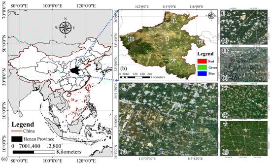
Figure 1.
Overview of the study area: (a) location of Henan Province; (b) true-color satellite image of Henan Province; (c–g) typical cultivated land areas in central, northern, western, southern, and eastern regions of Henan Province.
2.1.2. Data Resources
The data sources for this study include vegetation coverage data, topographic factors, climatic factors, and human activity factors. As shown in Table 1, the calculation of the CLUE index is based on FVC, with FVC data obtained from the National Tibetan Plateau Data Center, covering the period from 2000 to 2023. Given that May is a critical growth phase for Henan’s primary crop (wheat) from grain filling to maturity, when vegetation coverage is relatively stable and better reflects CLUE, the FVC data from each May is used to model the CLUI. The climatic and topographic factors include annual Average Temperature (Avg. Temp), Precipitation (Precip.), Digital Elevation Model (DEM), and slope data. For human activity factors, variables (e.g., Power Consumption (PC), Primary Industry (PI), Secondary Industry (SI), Tertiary Industry (TI), Gross Domestic Product (GDP), local fiscal gross budget expenditure (GBE), General Budget Revenue of Local Finance (GBR), Completed Investment in Residential Development (CIRD), Total Amount of Real Estate Development (TRED), Population Density (Pop. Dens.), Non-Agricultural Population (Non-Ag Pop.), and Registered Population (Reg. Pop.) were considered.

Table 1.
Factor and data sources.
2.2. Methods
2.2.1. Method for Constructing the CLUI
To assess the overall CLUE in Henan Province, this study introduced a CLUI. The calculated CLUI results were organized into three levels of research units: provincial cities, prefecture-level cities, and counties, based on a 250 m pixel resolution. The average CLUI value was calculated for each research unit by considering the number of pixels within each unit’s boundary, representing the overall CLUE within the area. The index calculation is based on FVC, derived from the Normalized Difference Vegetation Index (NDVI) using the pixel dichotomy method [51,52]. FVC effectively reflects the spatial distribution of vegetation cover on the surface, specifically as the proportion of land area covered by vegetation. This measure is crucial for quantifying CLUE and monitoring changes in FVC. To capture the detailed characteristics of vegetation cover changes, the study decomposed the FVC time series to extract its long-term trends and interannual fluctuations, forming the basis for modeling the CLUI [53,54]. The formula for calculating the CLUI is as follows [55]:
where FVC represents the Fractional Vegetation Cover, T denotes the long-term trend component, YF indicates the interannual fluctuation component, and σR is the standard deviation of the residuals. The formula first removes the long-term trend and interannual fluctuations, enabling standardized processing of the residuals to construct an index that reflects changes in CLUE. The standardized residual component becomes the CLUI, which visually reflects the temporal dynamics of CLUE in Henan Province. The technical workflow of this study is shown in Figure 2.

Figure 2.
Flow chart of technical route.
2.2.2. Method for Analyzing Trends in CLUE
To quantitatively analyze the trend in CLUE, this study employs the Sen-MK trend test method [56]. This non-parametric statistical method combines the Theil–Sen slope estimator with the Mann–Kendall significance test and is widely used for trend analysis of long-term time series data [57]. The Theil–Sen slope estimation is a robust trend estimation method that calculates the median slope between all possible pairs of points in the time series to determine the direction and intensity of data change. This approach effectively reduces the influence of outliers on trend assessment and is suitable for non-normally distributed data. The equation is as follows [58]:
The Mann–Kendall trend test is a non-parametric method used to assess the significance of trends in time series data. By ranking the time series and calculating a sign function, it determines whether there is a significant upward or downward trend in the sequence. Its advantages include not requiring the data to follow a normal distribution and being unaffected by outliers. The calculation equation is as follows:
In the spatiotemporal analysis of changes in vegetation coverage, the combined use of the Sen-MK trend test method enables a quantitative assessment of the rate of change and its significance in the time series. As shown in Table 2, CLUI is classified into nine categories:
Table 2.
Sen-MK test trend categories.
2.2.3. Machine Learning Regression Analysis Model (ANN, RF)
- ANN regression analysis based on genetic algorithm
ANN is a computational model inspired by biological nervous systems and is widely used for modeling and prediction of complex nonlinear relationships. In this study, ANN was used to analyze the importance of driving factors for changes in cultivated land vegetation coverage in Henan Province from 2000 to 2020. By constructing a multi-layered artificial neuron network, the ANN can handle the relationship between complex input variables and capture the potential impact of different factors on cultivated land vegetation coverage. The calculation process of the ANN can be expressed by the following equation [56,59]:
where xᵢ represents the input variable, ωᵢⱼ denotes the weight between the input layer and the hidden layer, and ωⱼ represents the weight from the hidden layer to the output layer. bⱼ and b are the bias terms for the hidden layer and output layer, respectively. To improve the optimization efficiency and accuracy of the model, a genetic algorithm is used to optimize the ANN parameters. In the genetic algorithm (GA), each individual represents a set of weights and bias terms for ANN, and ANN evaluates each individual’s performance using the following fitness function [60]:
Here, yₖ denotes the actual value, ŷₖ(ω, b) is the ANN’s predicted value, and N is the sample size. The genetic algorithm optimizes the weights (ω) and biases (b) by maximizing the fitness function, thereby enhancing the predictive performance of the ANN. To improve the model’s generalization ability and avoid overfitting, the input data was standardized to ensure consistency across variable scales [58].
- 2.
- RF regression analysis based on particle swarm optimization algorithm
In this study, the RF regression model improves prediction accuracy by integrating multiple decision trees, and the results of each decision tree are weighted and averaged to generate the final prediction value. Specifically, the prediction formula of RF is:
where ŷ is the final predicted value, T is the number of decision trees, and fₜ(x) represents the prediction result of the t-th decision tree. To mitigate the impact of initial hyperparameter settings, this study employs Particle Swarm Optimization (PSO) for hyperparameter tuning. The velocity update formula for Particle Swarm Optimization is as follows:
where represents the velocity of particle i in generation t + 1, ω is the inertia weight, c1 and c2 are learning factors, r1 and r2 are random numbers, is the best position of particle i, is the global best position, and is the current position of particle i. The position update formula for the particle is as follows:
PSO optimizes the RF model by iteratively updating particle velocity and position to identify the best hyperparameters, thereby improving model performance in driving factor analysis [61,62].
2.2.4. Important Analysis of Variables Based on SHAP
This study uses SHAP to assess variable importance in the ANN and RF models, evaluating how each driving factor affects changes in CLUE. Based on Shapley values from game theory, SHAP assigns a contribution value to each input variable, including topographic, climatic, and human activity factors. By calculating SHAP values, the study quantitatively evaluates the impact of these variables on CLUE trends, determining their average importance through marginal contributions to predictions across different scenarios:
Here, ϕi is the Shapley value of the i-th variable, N represents the set of all variables, S is a subset of variables, f(S) is the model prediction value for subset S, and f(S ∪ {i}) is the model prediction value when variable iii is added to subset S. This study uses SHAP to reveal both the global importance of variables and their specific contributions to individual predictions. It visualizes how each variable affects CLUE changes, providing an accurate assessment of their importance and uncovering complex nonlinear relationships between influencing factors and CLUE trends.
However, in this study, a comprehensive analysis of the driving factors affecting changes in CLUE in Henan Province from 2000 to 2020 was conducted by combining ANN and RF with the SHAP. Since SHAP values may differ significantly in range and scale across different models, directly comparing these values could lead to misleading conclusions. To further enhance the stability and accuracy of variable importance rankings and to ensure the reliability of results, this study normalized and averaged the variable importance results from the ANN and RF.
where SHAPvalue represents the calculated SHAP value for each variable, SHAP (ANN) denotes the SHAP value of variables calculated from the ANN model, and SHAP (RF) denotes the SHAP value of variables calculated from the RF model.
3. Results
3.1. Analysis of Spatiotemporal Evolution Characteristics of CLUI
3.1.1. The Overall CLUI Shows a Fluctuating Upward Trend
In Figure 3 and Table A1 in Appendix A, between 2000 and 2020, the changes in the CLUI in Henan Province showed significant inter-annual variation characteristics, with an overall fluctuating upward trend. In the past 20 years, CLUI has experienced many fluctuations, and the vegetation coverage has gradually increased from a lower level to a higher level. Especially after 2004, 2012, and 2016, the utilization rate of cultivated land improved significantly. Specifically, from 2000 to 2008, the utilization rate of cultivated land in Henan Province increased slowly and the vegetation coverage was low, indicating that the CLUE was greatly restricted at that time. After 2008, CLUI increased significantly, especially in the eastern and northern regions. By 2020, CLUI has reached a high level, and most of the province’s cultivated land areas show high vegetation coverage. From the perspective of spatial distribution, the improvement of CLUI in Henan Province has obvious spatial heterogeneity. The eastern plains area has obvious advantages due to its flat terrain and high CLUI; in comparison, the western and southern mountainous areas are limited by terrain, and their CLUE has improved more slowly. Overall, from 2000 to 2020, the cultivated land utilization rate in Henan Province showed an overall increase but significant regional differences.

Figure 3.
Interannual changes in CLUI in Henan Province from 2000 to 2020. (a) Representing the spatial differences of CLUI in Henan Province in 2000; (b) Representing the spatial differences of CLUI in Henan Province in 2002; (c) Representing the spatial differences of CLUI in Henan Province in 2004; (d) Representing the spatial differences of CLUI in Henan Province in 2006; (e) Representing the spatial differences of CLUI in Henan Province in 2008; (f) Representing the spatial differences of CLUI in Henan Province in 2010; (g) Representing the spatial differences of CLUI in Henan Province in 2012; (h) Representing the spatial differences of CLUI in Henan Province in 2014; (i) Representing the spatial differences of CLUI in Henan Province in 2016; (j) Representing the spatial differences of CLUI in Henan Province in 2018; (k) Representing the spatial differences of CLUI in Henan Province in 2020.
Figure 4 shows the interannual changes in the maximum and average values of the CLUI in Henan Province from 2000 to 2020. Among them, Figure 4a and Figure 4b, respectively, show the changing trend of the maximum value of CLUI and the changing trend of the average value and their corresponding linear regression models and 95% confidence intervals. During the research period, the maximum value of CLUI remained at a high level close to 1.0 in most years, especially reaching significant peaks in 2002, 2015, and 2018, indicating that the CLUE of some cultivated land reached extremely high levels in these years. The average CLUI gradually increased from approximately 0.85 in 2000 to approximately 0.87 in 2020, which means that the overall CLUE in Henan Province has improved.
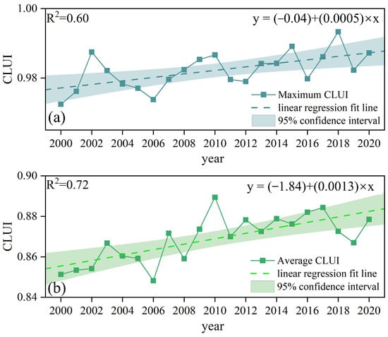
Figure 4.
Interannual change trend of CLUI index from 2000 to 2020: (a) represents the interannual change of the maximum value of CLUI, and (b) represents the interannual change of the average CLUI.
3.1.2. The CLUI Has Obvious Differences Between Years
In 2004 and 2010, the CLUI average reached a relatively high point, while there was a significant decline in 2006, 2008, and 2019. These fluctuations reflect the differences in CLUE between years. At the same time, there are also fluctuations in the maximum CLUI, e.g., slight decreases in 2006 and 2012. In the interannual changes of the average CLUI in Figure 4b, the average CLUI also shows a gradual upward trend. Comparing the changes in the maximum value and the average value, it can be found that the fluctuation range of the maximum value of CLUI is relatively large, while the fluctuation of the average value of CLUI is relatively stable. This shows that although some areas have achieved high CLUE in specific years, overall, the improvement in CLUE across the province has been relatively slow and balanced. The width of the confidence interval reflects the credibility of the model to changes in the data. Figure 4 shows that the width of the confidence interval changes over time, indicating that there is a certain uncertainty in the fluctuations of cultivated land utilization in different years. Overall, between 2000 and 2020, both the maximum and average values of CLUI showed an upward trend, and its linear regression model showed a significant positive slope, indicating that the CLUE of Henan Province has improved during the study period.
3.1.3. There Are Obvious Differences Between Regions in CLUI
In Figure 5 and Table A1, Table A2 and Table A3 in Appendix A, the spatial evolution trend of the CLUI in Henan Province from 2000 to 2020 is based on the Sen-MK trend test. A small part of Zhengzhou City in the middle and Shangqiu in the east show an obvious decreasing trend, especially Zhengzhou City. Figure 5a shows that the cultivated land utilization rate in most areas mainly decreases from slight to extreme (orange and red), only in some places. There is a small increase in the area. The situation in the eastern region is similar to that in the central region. The utilization rate of cultivated land has mainly declined in the past two decades, and a few areas have experienced slight degradation (yellow). This general downward trend shows that the central and eastern regions faced a more significant problem of insufficient utilization of cultivated land during the study period.

Figure 5.
CLUI Sen-MK trend test from 2000 to 2020: (a) represents central Henan Province; (b) represents northern Henan Province; (c) represents western Henan Province; (d) represents central Henan Province; (e) represents southern Henan Province.
The trend of cultivated land utilization in Hebi City in the north and Luoyang City in the west is more positive. In Hebi City, the overall cultivated land utilization rate remained stable and increased slightly, mainly in light green and light blue, indicating that the CLUE in this area increased slightly during the study period. The situation in Luoyang City is the most prominent, with dark blue covering most of the region, indicating that the cultivated land utilization rate in the west has increased significantly, and it is the region with the most positive changes in CLUE among the five regions. This improvement may be closely related to factors, (e.g., improvements in infrastructure, support from government policies, and advances in agricultural technology), in recent years, making Luoyang City a model for improving CLUE in the province.
The situation at the junction of Zhumadian City and Xinyang City in the southern region is more complicated. There are areas with significant increases (dark green) and areas with significant decreases (red and orange), showing obvious spatial imbalance. This fluctuation characteristic indicates that there are significant differences in CLUE in different regions. Overall, the cultivated land utilization rate in Henan Province showed strong spatial heterogeneity between regions from 2000 to 2020: it mainly decreased in the central and eastern parts, remained stable and slightly improved in the north, increased significantly in the west, and increased in the south. It shows complex fluctuations. The differences between different regions reflect the differences in agricultural development and land management policies within Henan Province.
3.2. Analysis of Driving Factors for Changes in CLUI
3.2.1. Screening of Main Driving Factors for Changes in CLUI
This study uses ANN optimized by genetic algorithm and RF optimized by particle swarm to conduct an in-depth analysis of the controlling factors of changes in cultivated land utilization in Henan Province from 2000 to 2020, aiming to reveal different driving factors. The importance of factors in the process of improving CLUE.
Table 3 and Table 4 show the comparison results of modeling parameters and accuracy indicators of ANN and RF models before and after optimization, respectively. For the ANN model, the hidden layer size before optimization is 10, the learning rate is 0.05, the regularization term is 0.01, the coefficient of determination (R2) of the model is 0.48, and the root mean square error (RMSE) is 0.007. After optimization, the hidden layer size was reduced to 5, the learning rate was reduced to 0.0214, the regularization term was increased to 0.0875, R2 was significantly improved to 0.78, and the RMSE was reduced to 0.001. Obviously, the optimized ANN model has significantly improved in terms of fitting accuracy and error control, which shows that the optimization of model parameters through genetic algorithms makes the model more efficient and accurately reflect the changing characteristics of cultivated land utilization.
Table 3.
Modeling parameters and accuracy indicators before and after ANN optimization.
Table 4.
Modeling parameters and accuracy indicators before and after RF optimization.
For the RF model, the parameters before optimization are set to the number of trees 100, the minimum leaf node is 5, the maximum depth is 20, the number of sampled predictors is 16, and the learning rate is 0.1. In the optimized model parameters, the number of trees is reduced to 54, the minimum leaf node is reduced to 1, the maximum depth is increased to 50, the number of sampled predictors is reduced to 8, and the learning rate is increased to 0.5. The R2 value of the model increased from 0.74 before optimization to 0.94, and the RMSE significantly decreased from 0.00007 to 0.000002. This shows that the adjustment of model parameters through the particle swarm optimization significantly improves the prediction accuracy of the model, allowing the RF to characterize dynamic changes more accurately in CLUE in Henan Province.
Figure 6 shows the ranking of the importance of variables in the model before and after optimization, reflecting the contribution of each variable to changes in cultivated land utilization. In Figure 6a,b, the importance ranking of variables before and after ANN model optimization is shown, respectively. The ranking of each variable in the model has changed significantly after optimization. Before optimization, variables (e.g., GBE, TRED, SI, and CIRD) had high importance in the model; after optimization, the influence of factors (e.g., GBR, SI, Pop. Dens., and Reg. Pop.) increased significantly. This shows that the optimized ANN model more prominently reflects the control effect of economic and social factors among human activity factors on cultivated land utilization. Similarly, Figure 6c,d show the ranking of variable importance before and after RF model optimization. Before optimization, variables (e.g., Precip, Pop. Dens., CIRD, and TI) have high importance in the model; but after optimization, factors (e.g., TI, Pop. Dens., Avg. Temp, and Reg. Pop.) influence has increased significantly. This shows that the optimized RF is more sensitive in reflecting socio-economic-related factors among human activity factors, and the importance of various economic activities and demographic data is further enhanced.
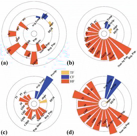
Figure 6.
Variable importance ranking chart before and after optimization: (a) represents the variable importance ranking before ANN optimization; (b) represents the variable importance ranking after ANN optimization; (c) represents the variable importance ranking before RF optimization; (d) represents RF. Ranking of variable importance after optimization.
To compare the importance of variables in different models more comprehensively, we normalized the variable importance results of the ANN and RF to the same range to eliminate the differences caused by different calculation scales. The normalized results can more accurately reflect the relative contribution of each variable in different models. In order to further improve the robustness and accuracy of variable ranking, the study generated the final comprehensive variable importance ranking by averaging the normalized results of the ANN and RF, as shown in Figure 7.

Figure 7.
Average variable importance ranking.
As can be seen from Figure 7, economic and social factors play the most significant role among human activity factors. In particular, factors (e.g., Pop. Dens., local fiscal revenue, and industrial output value play a major driving role in improving CLUE. At the same time, natural factors (e.g., Avg. Temp and Precip.) also play a certain supporting role in the environmental conditions of cultivated land productivity. The top seven main variables that contribute most significantly to changes in CLUE are “Pop. Dens.”, “GBR”, “SI”, “Reg. Pop.”, “GBE”, “PC” and “Avg. Temp.”. These results indicate that economic and social factors (e.g., Pop. Dens., GBR, and SI) play an important role in driving changes in CLUE.
Among them, “Pop. Dens.” has the highest average importance, reaching 0.95, which reflects that in areas with relatively concentrated populations, CLUE is significantly improved, which is related to the fact that population density directly affects the intensive use of land. Secondly, the average importance of “GBR” is 0.92, indicating that local government fiscal revenue plays an important role in promoting the improvement of cultivated land utilization. The importance of “Avg. Temp” is 0.84, showing that temperature, as an environmental condition, plays a key role in CLUE and has a direct impact on crop growth and cultivated land productivity. Furthermore, the average importance of “SI” is 0.89, indicating the significant impact of industrialization level on cultivated land utilization. The average importance of “Reg. Pop.” is 0.88, showing the comprehensive impact of Reg. Pop. on land resource demand and CLUE. The average importance of “CIRD” and “TI” is both 0.78, indicating that the rapid development of real estate development and the service industry has a certain impact on cultivated land utilization.
3.2.2. Analysis of Inter-Annual Changes in Main Driving Factors
Through an in-depth analysis of the main driving factors, the time evolution characteristics of the main driving factors in Henan Province from 2000 to 2020 can be systematically observed. As shown in Figure 8, overall, the inter-annual changes in each factor show a significant trend.
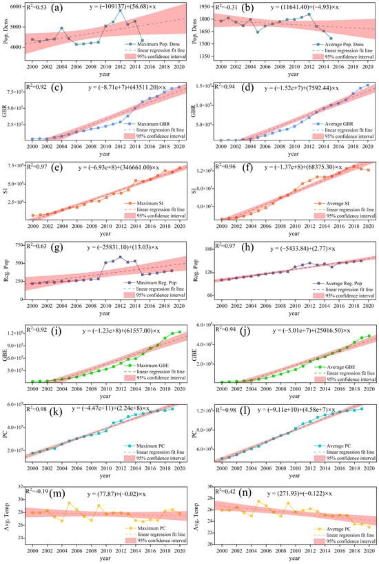
Figure 8.
Interannual changes of main factors: (a) represents the age change of the maximum value of Pop. Dens.; (b) represents the age change of the average value of Pop. Dens.; (c) represents the age change of the maximum value of GBR; (d) represents the age change of the average value of GBR; (e) represents the maximum SI value age change; (f) represents the SI average age change; (g) represents the Reg. Pop. maximum age change; (h) represents the Reg. Pop. average age change; (i) represents the GBE maximum age change; (j) represents the GBE average age change; (k) represents the age change of the maximum value of PC; (l) represents the age change of the average PC value; (m) represents the age change of the maximum value of Avg. Temp, and (n) represents the age change of the average value of Avg. Temp.
From 2000 to 2020, the maximum and average values of Pop. Dens. generally, show a steady upward trend. The maximum fitting degree is 0.53, while the fitting degree of the average value is 0.31, which shows that between different regions. There is obvious heterogeneity in the changes in population density, reflecting the differentiated characteristics of population agglomeration in different regions during this period. The maximum and average values of the Reg. Pop. also show a significant upward trend, with fitting degrees of 0.63 and 0.97, respectively, indicating that the overall population growth is significant and stable.
Both GBR and GBE showed significant growth during the study period. The fitting degree of the changing trend of the maximum value and average value of GBR is 0.92 and 0.94, respectively, while the fitting degree of GBE also reaches a similar level. These high-fitting degrees indicate that fiscal budget revenue and expenditure show a highly consistent and significant growth trend across the province. Similarly, the maximum and average trend-fitting degrees of SI are 0.97 and 0.96, respectively, showing the steady advancement of industrialization during the study period. Both the maximum value and the average value of PC show a significant linear upward trend, and the fitting degrees for them are both 0.98, which further reflects the general improvement of the level of industrialization. The maximum and average values of Avg. Temp. generally show a downward trend, and the fitting degrees are 0.19 and 0.42, respectively, reflecting the large fluctuations and regional differences in temperature changes. During the study period, the changes in Avg. Temp were complex and showed large uncertainties between different years and regions.
3.2.3. Correlation Analysis Between Main Driving Factors and CLUE
According to the spatial correlation analysis between the main driving factors and CLUE in Figure 9, it can be found that human activity factors have a significant and concentrated impact on CLUE, while the effects of terrain and climate factors are relatively scattered. According to the correlation between each driving factor and CLUE, these factors can be classified into four categories: strong correlation, weak correlation, no correlation, and negative correlation.
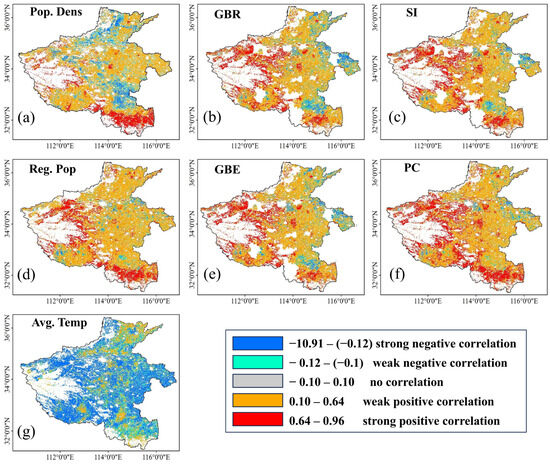
Figure 9.
Correlation analysis between main driving factors and CLUI: (a) represents the correlation analysis between Pop. Dens. and CLUE; (b) represents the correlation analysis between GBR and CLUE; (c) represents the correlation analysis between SI and CLUI; (d) represents the correlation analysis between Reg. Pop. and CLUI; (e) represents the correlation analysis between GBE and CLUI; (f) represents the correlation analysis between PC and CLUI; (g) represents the correlation analysis between Avg. Temp and CLUI.
Among the human activity factors, economic and demographic factors have the most significant impact on CLUE. Pop. Dens., GBR, GBE and PC show strong positive correlation and have obvious spatial characteristics (Figure 9a,b,e,f). In the cities of Zhengzhou, Xuchang and Kaifeng in central Henan Province and Xinyang City in the south (research unit correlation analysis Appendix A), CLUE shows a strong positive correlation (red area) with these factors, reflecting that human activities are closely related to CLUE. In Puyang City in the north of Henan Province and Shangqiu City in the west, the correlation of these factors is weak or even negative (blue area), indicating that human activities in these areas have less impact on CLUE. In these areas, GBR, PC, and Pop. Dens. do not have a significant positive correlation with improvements in CLUE.
The spatial correlations of SI and Reg. Pop. in Figure 9c,d show regional differences. The output value of the SI in Luoyang City and Nanyang City in the west of Henan Province and Xinyang City in the south shows a positive correlation with CLUE (red and orange areas), while in Zhengzhou City in the center of Henan Province and Shangqiu City in the north the performance is as follows Weak or negative correlation (light blue and blue areas). The Reg. Pop. shows a positive correlation in some areas of Xinyang City in southern Henan Province and Pingdingshan City in the central part of the province. However, in Kaifeng City in western Henan Province, the increase in Reg. Pop. does not bring about an obvious improvement in CLUE, and some areas even show a negative correlation. The correlation between Avg. Temp. and CLUE (Figure 9g) shows a positive correlation in Anyang City in the north of Henan Province and Xinyang City in the south, while it shows a negative correlation in most areas of Henan Province. This shows that there are regional differences in the impact of Avg. Temp on CLUE, which may be related to climatic conditions and agricultural production methods in different regions.
4. Discussion
4.1. Impact of Terrain and Climate Factors on CLUE
The effects of terrain and climate factors on CLUE show significant differences in different regions. Through the analysis of the CLUI in Henan Province, it can be found that topographic factors (e.g., slope and DEM) have a relatively limited impact on the province’s CLUE. Most areas in Henan Province are plains with small terrain changes, therefore, their contribution to CLUE is low. However, in mountainous and hilly areas (e.g., western Henan Province), slope and elevation have certain constraints on the use of cultivated land. The complexity of the terrain makes the level of mechanization in these areas low, and it is difficult to improve CLUE. This finding has certain similarities and differences with research results in other regions. In Yunnan Province in southern China, research shows that natural factors have a certain impact on CLUE, but agricultural production conditions (e.g., effective irrigation area and total power of agricultural machinery) have a more significant impact on CLUE [63,64]. The terrain of Yunnan Province is complex, with a large proportion of mountains and plateaus. The impact of terrain factors on agricultural mechanization and irrigation conditions is more prominent, resulting in a more obvious impact of terrain factors on CLUE [65]. In contrast, northeastern regions (e.g., Jilin Province), China’s main grain-producing areas, have relatively flat terrain and are suitable for large-scale mechanized operations [66,67,68]. The topography has fewer constraints in CLUE. However, cold climate conditions may limit crop growth cycles and negatively impact CLUE. This is consistent with the inhibitory effect of Avg. Temp on CLUE in the northern and western regions of Henan Province, indicating that climate factors have an important impact on CLUE in cold areas.
4.2. Impact of Human Activity Factors on CLUE
Human activity factors have a significant driving effect on the improvement of CLUE. It can be seen from the ranking of variable importance (Figure 7) that Pop. Dens., GBR, SI, Reg. Pop., GBE and PC are the factors that have the greatest impact on CLUE. The impact of these factors on CLUE in different regions reflects obvious regional differences. First, Pop. Dens. shows a significant positive correlation with CLUE in areas with relatively concentrated populations, e.g., central and southern Henan. This shows that the agglomeration of population resources helps to manage and utilize cultivated land resources more effectively. Sufficient labor allows the land to be cultivated intensively, improving land productivity and utilization efficiency. This finding is consistent with research results in areas, e.g., Jilin Province, where areas with higher population density also have higher CLUE. The main reason is that labor input promotes the intensification of agricultural production [5].
Secondly, local fiscal revenue and expenditure have played an important role in promoting CLUE. Financial investment is mainly used for the construction of agricultural infrastructure, the improvement of cultivated land water conservancy facilities, and the promotion of agricultural mechanization, thus directly improving the utilization of land, especially in aspects, e.g., reservoir expansion, river management, and water diversion projects [69]. During 2023–2024, Henan Province has 454 projects in seven categories including flood prevention and disaster reduction, irrigation area renovation, water ecological management, urban and rural water supply, water system connectivity, water environment improvement, and digital twins, with a total investment of CNY 51.724. For example, in Xinyang City in southern Henan Province, Pingdingshan City in central China, and Nanyang City in southwestern Henan Province, the investment in major water conservancy projects was CNY 9.751, CNY 8.618, and CNY 5.917, respectively. By increasing fiscal expenditures, agricultural production capacity was significantly improved, resulting in a significant increase in CLUE in these areas during the study period. This echoes the research in Yunnan Province, where effective irrigated areas and the total power of agricultural machinery are the main factors in improving CLUE, and financial investment is crucial to improvements in these aspects. For example, the Xixiayuan Project is in Henan Province in the middle reaches of the mainstream of the Yellow River. After the project is completed, it will be connected to the four major water diversion areas of Xixiayuan, Wujia, Renmin Shengli Canal and Dagong to divert water from the Yellow River into the irrigation area, with an annual water diversion of 213 million cubic meters. New developments the irrigated area is 310,000 acres, and the irrigated area of 1.4 million acres will be supplemented by Wujia Irrigation District, Renmin Shengli Canal Irrigation District and Dagong Irrigation District, which can increase grain production capacity by 410 million kilograms every year.
The output value of the SI has a positive correlation with CLUE in some areas, indicating that capital flows brought about by industrial development help improve agricultural productivity. Industrialization has promoted agricultural mechanization and technological progress, and improved CLUE. However, this impact differs between the central, western, and northern regions of Henan Province. The increase in the level of industrialization in some regions has led to a reduction in the agricultural labor force, as the labor force is attracted to the industrial sector, resulting in a shortage of agricultural production personnel, which has a negative impact in CLUE. For example, in Xuchang City, located in the central part of Henan Province, in 2023, the added value of the SI was CNY 139.89, an increase of 1.6%. At the end of 2023, the city’s permanent population was 4.383 million, including 2.460 million urban residents and 1.923 million rural residents; The urbanization rate of the permanent population was 56.12%, an increase of 0.94 percentage points from the end of the previous year. The permanent population in rural areas decreased, and industrial development attracted the agricultural population [70,71].
In addition, economic and demographic factors (e.g., GDP, PC, Reg. Pop.) also have an important impact on CLUE. However, rapid economic development and urbanization have caused many rural labor forces to migrate to cities, resulting in a shortage of agricultural labor and affecting agricultural production efficiency. In Henan Province, the impact of urbanization on CLUE presents such complexity. On the one hand, it promotes agricultural modernization, and on the other hand, it may lead to labor shortages. Therefore, there is a need to balance the relationship between industrial development, urbanization and agricultural land use when formulating future agricultural and land management policies. Financial support for agriculture should be strengthened, agricultural mechanization and technological progress should be promoted, and CLUE should be improved. At the same time, we must prevent excessive industrialization and urbanization from causing the loss of agricultural labor and affecting agricultural production. Drawing on the experience of other regions, Sichuan Province, for example, while promoting urbanization, has strengthened large-scale agricultural operations and promoted the coordinated improvement of high-quality agricultural development and CLUE.
4.3. Policy and Management Recommendations
Based on the above analysis of the inter-annual changes and main driving factors of CLUE in Henan Province, in order to effectively improve the CLUE in Henan Province, the following policy recommendations are put forward to ensure food security and promote sustainable agricultural development [72]. In response to the complex terrain and unfavorable agricultural production conditions in the western region of Henan Province, infrastructure construction, especially the construction of terraces and irrigation systems, should be stepped up to effectively prevent soil erosion. At the same time, small machinery suitable for mountainous operations should be introduced to improve CLUE. In the central and eastern regions, we should continue to strictly implement the cultivated land red line policy to prevent non-agricultural construction from occupying cultivated land, and actively promote the crop rotation and fallow system and high-standard cultivated land construction to improve soil fertility and thereby improving the quality of cultivated land and CLUE. The promotion of agricultural mechanization and water-saving irrigation technology is also crucial. Especially in the eastern region, high-efficiency water-saving technologies (e.g., drip irrigation and sprinkler irrigation), should be promoted through increased financial support to ensure the stability and efficiency of agricultural production.
In regions with higher population densities (e.g., the central and eastern regions), emphasis should be placed on optimizing land management and preventing degradation caused by overuse of land [73]. Especially in the process of industrialization and urbanization, it is necessary to scientifically plan land use, clarify the protection scope of agricultural land, and prevent high-quality cultivated land from being encroached upon. We should encourage the integrated development of agriculture and industry, support emerging industries (e.g., agricultural product processing and agricultural tourism), extend the agricultural industry chain, and achieve coordinated development of agriculture and industry.
In areas with weak infrastructure, financial support for agricultural mechanization and water-saving irrigation facilities should continue to be increased to cope with sudden drought conditions [74]. For example, in June 2024, the area that could not be sown in Henan Province due to drought reached 3.23 million acres. In total, 72 national weather stations in 16 prefectures and cities in Henan, including Anyang, Hebi, Jiaozuo and Kaifeng, have monitored meteorological droughts that have reached severe drought levels or above and have lasted for several days. The Henan Provincial Department of Water Resources has strengthened the dispatching and management of irrigation water sources, increased the discharge flow according to the needs of downstream drought relief irrigation, and maximized the guarantee of irrigation water in the irrigation areas. Henan Electric Power Company prioritizes ensuring electricity demand for drought relief and increases the frequency of inspections and inspections of well power supply facilities. Electricity is an important energy source for modern agriculture. In order to ensure the energy supply for agricultural production, it is recommended to improve the construction level of rural power grids and ensure the stability of electricity consumption for agricultural production, especially during critical farming seasons. At the same time, the use of clean energy (e.g., solar energy) should be encouraged to reduce dependence on traditional energy and promote the development of green agriculture. In addition, for regions with rapid industrialization (e.g., the central and eastern regions), it is recommended that policymakers strike an effective balance between industrialization and agricultural development to prevent industrial development from over-occupying agricultural land and labor to ensure the stability of agricultural production [75,76].
In the future, agricultural development in Henan Province will need to rely on inter-regional cooperation and experience sharing, especially between efficient and backward areas. To promote this, Henan can focus on the following measures: First, industrial collaboration by leveraging its agricultural foundation and partnering with modern agricultural enterprises and industrial capital from technologically advanced regions. This can be achieved through joint park development and extending the industrial chain, with the goal of building agricultural production bases that improve both production and management levels. Second, Henan should strengthen agricultural openness and external cooperation by implementing institutional strategies that promote multi-level, diversified collaboration. This includes optimizing agricultural foreign cooperation, establishing open platforms, and enhancing international competitiveness to expand agricultural international cooperation. Finally, Henan can enhance agricultural science and technology cooperation by partnering with key agricultural research institutes and universities. Joint efforts should focus on breeding quality seeds, in-depth agricultural product processing, and agricultural machinery innovation. These measures will help improve agricultural management, support sustainable development, and strengthen food security and agricultural modernization in Henan.
5. Conclusions
This study comprehensively analyzed the spatiotemporal evolution characteristics of CLUE in Henan Province from 2000 to 2020 by constructing a CLUE index based on vegetation coverage, combined with Theil–Sen slope and Mann–Kendall trend test, and based on the optimized ANN and The RF evaluates the combined effects of terrain, climate and human activity factors. The results show that: (1) From 2000 to 2020, the CLUI of Henan Province generally showed a fluctuating upward trend, especially after 2004, 2012 and 2016, which increased significantly. The CLUI in the eastern plains is higher, while the improvement in mountainous areas is slower due to terrain restrictions. (2) Between 2000 and 2020, the CLUI in Henan Province showed obvious spatial differences: the central and eastern regions mainly decreased, and the northern Maintained a stable slight increase, with a significant improvement in the west, while the south fluctuated greatly, showing significant spatial imbalance. (3) Henan Province’s CLUE is mainly affected by human activity factors, especially economic and demographic factors among human activity factors, showing significant positive correlation in Zhengzhou, Xuchang and other places. However, human activities in Puyang in the north and Shangqiu in the west have little impact on CLUE, or even have a negative correlation. The impact of SI output value and Reg. Pop. varies significantly in different regions. For example, Luoyang and Xinyang have a positive correlation, while Zhengzhou and Shangqiu have a weak or negative correlation. At the same time, the impact of Avg. Temp on CLUE has significant regional differences, with a positive correlation in Anyang and Xinyang, and a negative correlation in other regions. The findings of this study provide a scientific basis for future land management and agricultural policy formulation in Henan Province, especially in improving regional CLUE and promoting sustainable agricultural development.
Author Contributions
Project administration and funding acquisition, H.Z. and X.M.; writing—review and editing, H.Z., T.J. and C.Z.; writing—original draft and methodology, H.Z., K.L. and C.Z.; investigation, M.W. and K.L. All authors have read and agreed to the published version of the manuscript.
Funding
This research was funded by Graduate Education Innovation Plan Project of the Education Department of Xinjiang Uygur Autonomous Region (grant number XJ2024G083); National Natural Science Foundation of China (grant number 42201390 and 42461052); the University of Basic Scientific Business Fees for Scientific Research Projects in the Xinjiang Uygur Autonomous Region (grant number XJEDU2022P014); the Open Project of Key Laboratory in the Xinjiang Uygur Autonomous Region (grant number 2023D04051); the Tianchi Doctoral Program in the Xinjiang Uygur Autonomous Region (grant number TCBS202127); the International Cooperation Scientific Research Project of the Ministry of Education’s “Chunhui Plan” (grant number HZKY20220609); the State Key Laboratory of Desert and Oasis Ecology, Xinjiang Institute of Ecology and Geography, Chinese Academy of Sciences (grant number G2023-02-05); the General Project of the Central Asian Research Institute from Xinjiang University (grant number 24FPY003); and the Key Research and Development Program of the Xinjiang Uygur Autonomous Region (grant number 2022B02003 and 2022B01012).
Data Availability Statement
The data provided in this study are available upon request from the corresponding author. The data are not publicly available as they are being collated.
Conflicts of Interest
The authors declare no conflicts of interest.
Appendix A
Table A1.
Statistical results of the overall CLUI and trend of 18 provincial municipalities and provincial-level cities in Henan Province in 2000 and 2020.
Table A1.
Statistical results of the overall CLUI and trend of 18 provincial municipalities and provincial-level cities in Henan Province in 2000 and 2020.
| Provincial Municipalities | 2000CLUI | 2020CLUI | Sen’s Slope |
|---|---|---|---|
| Anyang city | 0.0388 | 0.0409 | 0.1331 |
| Hebi city | 0.0901 | 0.0951 | 0.3579 |
| Pu yang city | 0.0647 | 0.0681 | 0.1583 |
| Xinxiang city | 0.0263 | 0.0273 | 0.0832 |
| Jiaozuo city | 0.0565 | 0.0584 | 0.1735 |
| Jiyuan city | 0.3103 | 0.3268 | 1.1702 |
| Zhengzhou city | 0.1433 | 0.1496 | 0.3394 |
| Sanmenxia city | 0.0411 | 0.0438 | 0.1654 |
| Luoyang city | 0.0803 | 0.0843 | 0.2942 |
| Xuchang city | 0.0112 | 0.0115 | 0.0404 |
| Pingdingshan city | 0.0810 | 0.0840 | 0.2933 |
| Zhoukou city | 0.0107 | 0.0106 | 0.0133 |
| Luohe city | 0.0020 | 0.0020 | 0.0067 |
| Zhumadian city | 0.0186 | 0.0191 | 0.0646 |
| Xinyang city | 0.7075 | 0.7206 | 2.4567 |
| Shangqiu city | 0.5141 | 0.5208 | 0.3736 |
| Nanyang city | 0.6071 | 0.6234 | 1.9629 |
| Kaifeng city | 0.0742 | 0.0779 | 0.2139 |
Table A2.
Statistical results of the overall CLUI and trend of 21 county-level cities in Henan Province in 2000 and 2020.
Table A2.
Statistical results of the overall CLUI and trend of 21 county-level cities in Henan Province in 2000 and 2020.
| County-Level Cities | 2000CLUI | 2020CLUI | Sen’s Slope |
|---|---|---|---|
| Linzhou city | 0.2897 | 0.3067 | 0.9606 |
| Anyang city | 0.0388 | 0.0409 | 0.1331 |
| Huixian city | 0.3074 | 0.3197 | 0.7933 |
| Qinyang city | 0.1451 | 0.1496 | 0.3232 |
| Mengzhou city | 0.1599 | 0.1654 | 0.2956 |
| Xingyang city | 0.2237 | 0.2362 | 0.8327 |
| Gongyi city | 0.1476 | 0.1564 | 0.6559 |
| Yima city | 0.0232 | 0.0246 | 0.1017 |
| Yancity city | 0.2336 | 0.2454 | 0.9068 |
| Lingbao city | 0.4597 | 0.4828 | 1.5452 |
| Xinmi city | 0.2425 | 0.2576 | 1.0817 |
| Xinzheng city | 0.2384 | 0.2471 | 0.7253 |
| Dengfeng city | 0.2942 | 0.3096 | 1.3089 |
| Yuzhou city | 0.3900 | 0.4015 | 1.2880 |
| Ruzhou city | 0.4367 | 0.4560 | 1.6331 |
| Changge city | 0.1980 | 0.1998 | 0.3631 |
| Yongcheng city | 0.6452 | 0.6536 | 0.5266 |
| Xiangcheng city | 0.3416 | 0.3415 | 0.3085 |
| Wugang city | 0.1410 | 0.1449 | 0.4829 |
| Dengzhou city | 0.7987 | 0.8141 | 1.5561 |
| Weihui city | 0.2011 | 0.2094 | 0.4857 |
Table A3.
Statistical results of the overall CLUI and trends in 89 counties in Henan Province in 2000 and 2020.
Table A3.
Statistical results of the overall CLUI and trends in 89 counties in Henan Province in 2000 and 2020.
| County | 2000CLUI | 2020CLUI | Sen’s Slope |
|---|---|---|---|
| Anyang county | 0.3792 | 0.3978 | 0.7077 |
| Nanle county | 0.1848 | 0.1934 | 0.1949 |
| Neihuang county | 0.3815 | 0.3958 | 0.6545 |
| Taiqian county | 0.1210 | 0.1279 | 0.1977 |
| Qingfeng county | 0.2891 | 0.3033 | 0.4368 |
| Tangyin county | 0.2134 | 0.2231 | 0.2020 |
| Fan county | 0.1760 | 0.1845 | 0.2239 |
| Xun county | 0.3586 | 0.3776 | 0.4962 |
| Puyang county | 0.4462 | 0.4694 | 0.5741 |
| Hua county | 0.5856 | 0.6177 | 0.6454 |
| Xiuwu county | 0.1324 | 0.1371 | 0.3294 |
| Yanjin county | 0.3080 | 0.3215 | 0.6236 |
| Changyuan county | 0.3173 | 0.3348 | 0.4843 |
| Bo’ai county | 0.1101 | 0.1130 | 0.1934 |
| Huojia county | 0.1490 | 0.1535 | 0.3298 |
| Wuzhi county | 0.2567 | 0.2646 | 0.4358 |
| Wen county | 0.1552 | 0.1595 | 0.2020 |
| Lankao county | 0.3252 | 0.3391 | 0.3864 |
| Zhongmou county | 0.4045 | 0.4151 | 0.4354 |
| Mengjin county | 0.2212 | 0.2344 | 0.9106 |
| Minquan county | 0.3722 | 0.3776 | 0.2120 |
| Qi county | 0.4085 | 0.4228 | 0.8408 |
| Yiyang county | 0.4325 | 0.4541 | 1.8080 |
| Ningling county | 0.2558 | 0.2610 | 0.3522 |
| Yucheng county | 0.4981 | 0.5073 | 0.2937 |
| Luoning county | 0.3813 | 0.4055 | 1.6350 |
| Weishi county | 0.4237 | 0.4347 | 0.9862 |
| Tongxu county | 0.2630 | 0.2710 | 0.6207 |
| Sui county | 0.2893 | 0.2933 | 0.3113 |
| Yichuan county | 0.3129 | 0.3253 | 1.2001 |
| Xiayi county | 0.4639 | 0.4718 | 0.2229 |
| Lushi county | 0.2737 | 0.2950 | 1.2158 |
| Ruyang county | 0.2069 | 0.2170 | 0.8004 |
| Song county | 0.3167 | 0.3364 | 1.3370 |
| Fugou county | 0.3986 | 0.4089 | 0.8341 |
| Taikang county | 0.5898 | 0.6061 | 0.9805 |
| Zhecheng county | 0.3419 | 0.3468 | 0.3051 |
| Yanling county | 0.2950 | 0.3121 | 1.1150 |
| Luanchuan county | 0.1194 | 0.1246 | 0.4287 |
| Jia county | 0.2054 | 0.2103 | 0.6117 |
| Xuchang county | 0.3205 | 0.3275 | 0.7067 |
| Luyi county | 0.4020 | 0.4072 | 0.4686 |
| Baofeng county | 0.2233 | 0.2298 | 0.6540 |
| countygcheng county | 0.3008 | 0.3057 | 0.7324 |
| Lushan county | 0.4105 | 0.4291 | 1.6179 |
| Linying county | 0.2495 | 0.2584 | 0.7220 |
| Xihua county | 0.3920 | 0.4028 | 0.7058 |
| Huaiyang county | 0.4544 | 0.4675 | 1.1663 |
| Dancheng county | 0.4981 | 0.5077 | 0.6915 |
| Xixia county | 0.2296 | 0.2429 | 0.9615 |
| Ye county | 0.4261 | 0.4372 | 1.1198 |
| Yancheng county | 0.3156 | 0.3267 | 0.8203 |
| Shangshui county | 0.4243 | 0.4336 | 0.6740 |
| Nanzhao county | 0.3899 | 0.4089 | 1.7015 |
| Wuyang county | 0.2269 | 0.2328 | 0.5808 |
| Fangcheng county | 0.6735 | 0.6968 | 2.5494 |
| Neicountyg county | 0.3511 | 0.3639 | 1.0518 |
| Shenqiu county | 0.3363 | 0.3369 | 0.2837 |
| Xiping county | 0.3605 | 0.3699 | 0.8089 |
| Shangcai county | 0.4942 | 0.5038 | 1.0119 |
| Xichuan county | 0.4097 | 0.4332 | 1.4168 |
| Zhenping county | 0.4028 | 0.4139 | 1.1402 |
| Suiping county | 0.3666 | 0.3727 | 0.8745 |
| Runan county | 0.5127 | 0.5201 | 1.0989 |
| Pingyu county | 0.4127 | 0.4195 | 0.6488 |
| Biyang county | 0.6483 | 0.6657 | 2.6711 |
| Sheqi county | 0.3835 | 0.3873 | 0.9339 |
| Xincai county | 0.4316 | 0.4361 | 0.4843 |
| Tanghe county | 0.8335 | 0.8388 | 1.9943 |
| Xinye county | 0.3576 | 0.3681 | 1.1977 |
| Zhengyang county | 0.6354 | 0.6252 | 0.3798 |
| Tongbai county | 0.3880 | 0.4086 | 1.6944 |
| Xi county | 0.5883 | 0.5867 | 0.4686 |
| Huaibin county | 0.3817 | 0.3876 | 0.6036 |
| Gushi county | 0.8577 | 0.8801 | 2.7072 |
| Huangchuan county | 0.5658 | 0.5873 | 1.9862 |
| Luoshan county | 0.5529 | 0.5668 | 2.1288 |
| Guangshan county | 0.5523 | 0.5729 | 2.2776 |
| Shangcheng county | 0.4316 | 0.4441 | 1.5271 |
| Xin county | 0.1299 | 0.1350 | 0.5162 |
| Xincountyg county | 0.1506 | 0.1564 | 0.3612 |
| Yuanyang county | 0.3930 | 0.4089 | 0.8080 |
| Queshan county | 0.4910 | 0.5016 | 1.8161 |
| Qi county | 0.1094 | 0.1138 | 0.1735 |
| Mianchi county | 0.2735 | 0.2889 | 1.1502 |
| Xin’an county | 0.2464 | 0.2601 | 1.0989 |
| Shan county | 0.3021 | 0.3223 | 1.2296 |
| Kaifeng county | 0.4904 | 0.5130 | 1.3883 |
| Fengqiu county | 0.3800 | 0.4003 | 0.5841 |
Table A4.
Correlation results of main driving factors in 18 provincial municipalities and provincial municipalities in Henan Province.
Table A4.
Correlation results of main driving factors in 18 provincial municipalities and provincial municipalities in Henan Province.
| Provincial Municipalities | Pop. Dens | GBR | SI | Reg. Pop | GBE | PC | Avg. Temp |
|---|---|---|---|---|---|---|---|
| Anyang city | 0.0409 | 0.0001 | 0.0000 | 0.0215 | 0.0002 | 0.0241 | −0.0144 |
| Hebi city | 0.0951 | 0.0093 | 0.0220 | 0.0633 | 0.0094 | 0.0658 | −0.0307 |
| Pu yang city | 0.0681 | 0.0139 | 0.0320 | 0.0291 | 0.0157 | 0.0274 | −0.0074 |
| Xinxiang city | 0.0273 | 0.0109 | 0.0145 | 0.0109 | 0.0108 | 0.0144 | −0.0083 |
| Jiaozuo city | 0.0584 | 0.0020 | 0.0017 | 0.0199 | 0.0020 | 0.0315 | −0.0214 |
| Jiyuan city | 0.3268 | 0.2157 | 0.2287 | 0.0020 | 0.2256 | 0.2246 | −0.1326 |
| Zhengzhou city | 0.1496 | 0.0198 | 0.0272 | 0.0367 | 0.0192 | 0.0612 | −0.0436 |
| Sanmenxia city | 0.0438 | 0.0025 | 0.0026 | 0.0155 | 0.0026 | 0.0299 | −0.0161 |
| Luoyang city | 0.0843 | 0.0098 | 0.0172 | 0.0601 | 0.0098 | 0.0568 | −0.0397 |
| Xuchang city | 0.0115 | 0.0013 | 0.0020 | 0.0047 | 0.0016 | 0.0071 | −0.0034 |
| Pingdingshan city | 0.0840 | 0.0125 | 0.0127 | 0.0569 | 0.0106 | 0.0573 | −0.0224 |
| Zhoukou city | 0.0106 | 0.0001 | 0.0001 | 0.0029 | 0.0001 | 0.0031 | −0.0003 |
| Luohe city | 0.0020 | 0.0003 | 0.0004 | 0.0012 | 0.0003 | 0.0016 | −0.0007 |
| Zhumadian city | 0.0191 | 0.0002 | 0.0002 | 0.0107 | 0.0002 | 0.0129 | −0.0079 |
| Xinyang city | 0.7206 | 0.0049 | 0.0075 | 0.5253 | 0.0061 | 0.5424 | −0.1148 |
| Shangqiu city | 0.5208 | −0.0010 | 0.0008 | 0.1317 | 0.0005 | 0.0886 | −0.1085 |
| Nanyang city | 0.6234 | 0.0116 | 0.0101 | 0.3254 | 0.0114 | 0.3783 | −0.2602 |
| Kaifeng city | 0.0779 | 0.0047 | 0.0069 | 0.0239 | 0.0048 | 0.0393 | −0.0241 |
Table A5.
Correlation results of main driving factors in 21 county-level cities in Henan Province.
Table A5.
Correlation results of main driving factors in 21 county-level cities in Henan Province.
| County-Level Cities | Pop. Dens | GBR | SI | Reg. Pop | GBE | PC | Avg. Temp |
|---|---|---|---|---|---|---|---|
| Linzhou city | 0.3067 | 0.1671 | 0.1629 | 0.1744 | 0.1690 | 0.1742 | −0.1331 |
| Anyang city | 0.0409 | 0.0001 | 0.0000 | 0.0215 | 0.0002 | 0.0241 | −0.0144 |
| Huixian city | 0.3197 | 0.1589 | 0.1697 | 0.1463 | 0.1476 | 0.1637 | −0.0879 |
| Qinyang city | 0.1496 | 0.0569 | 0.0634 | 0.0544 | 0.0607 | 0.0646 | −0.0162 |
| Mengzhou city | 0.1654 | 0.0506 | 0.0529 | 0.0566 | 0.0516 | 0.0634 | −0.0155 |
| Xingyang city | 0.2362 | 0.1412 | 0.1466 | 0.1115 | 0.1381 | 0.1543 | −0.0956 |
| Gongyi city | 0.1564 | 0.1091 | 0.1175 | 0.0999 | 0.0998 | 0.1290 | −0.0544 |
| Yima city | 0.0246 | 0.0196 | 0.0177 | 0.0129 | 0.0196 | 0.0206 | −0.0132 |
| Yancity city | 0.2454 | 0.0237 | 0.0518 | 0.1709 | 0.0240 | 0.1641 | −0.1092 |
| Lingbao city | 0.4828 | 0.2771 | 0.2592 | 0.1831 | 0.2708 | 0.2812 | −0.0841 |
| Xinmi city | 0.2576 | 0.2117 | 0.2192 | 0.1801 | 0.1971 | 0.2209 | −0.1146 |
| Xinzheng city | 0.2471 | 0.1280 | 0.1357 | 0.1053 | 0.1251 | 0.1294 | −0.0963 |
| Dengfeng city | 0.3096 | 0.2495 | 0.2548 | 0.1871 | 0.2529 | 0.2529 | −0.1447 |
| Yuzhou city | 0.4015 | 0.2337 | 0.2349 | 0.1592 | 0.2490 | 0.2522 | −0.1305 |
| Ruzhou city | 0.4560 | 0.3132 | 0.3173 | 0.3129 | 0.3142 | 0.3141 | −0.2047 |
| Changge city | 0.1998 | 0.0615 | 0.0712 | 0.0245 | 0.0720 | 0.0944 | −0.0228 |
| Yongcheng city | 0.6536 | 0.0439 | 0.1901 | 0.1956 | 0.0422 | 0.1512 | −0.2089 |
| Xiangcheng city | 0.3415 | 0.0558 | 0.0879 | 0.1006 | 0.0721 | 0.1198 | −0.0962 |
| Wugang city | 0.1449 | 0.0785 | 0.0710 | 0.0947 | 0.0835 | 0.0972 | −0.0359 |
| Dengzhou city | 0.8141 | 0.3668 | 0.2614 | 0.1730 | 0.3593 | 0.3205 | −0.4146 |
| Weihui city | 0.2094 | 0.0751 | 0.0517 | 0.0787 | 0.0726 | 0.0957 | −0.0108 |
Table A6.
Correlation results of main driving factors in 21 county-level cities in Henan Province.
Table A6.
Correlation results of main driving factors in 21 county-level cities in Henan Province.
| County | Pop. Dens | GBR | SI | Reg. Pop | GBE | PC | Avg. Temp |
|---|---|---|---|---|---|---|---|
| Anyang county | 0.3978 | 0.1072 | 0.1181 | 0.1520 | 0.1038 | 0.1515 | −0.0411 |
| Nanle county | 0.1934 | 0.0017 | 0.0411 | 0.0520 | 0.0169 | 0.0395 | 0.0262 |
| Neihuang county | 0.3958 | 0.0627 | 0.1565 | 0.1749 | 0.0959 | 0.1529 | −0.0035 |
| Taiqian county | 0.1279 | 0.0102 | 0.0435 | 0.0542 | 0.0111 | 0.0446 | 0.0076 |
| Qingfeng county | 0.3033 | 0.0364 | 0.0800 | 0.1074 | 0.0564 | 0.0859 | 0.0046 |
| Tangyin county | 0.2231 | 0.0245 | 0.0654 | 0.0527 | 0.0284 | 0.0380 | 0.0149 |
| Fan county | 0.1845 | 0.0113 | 0.0379 | 0.0687 | 0.0198 | 0.0427 | 0.0130 |
| Xun county | 0.3776 | 0.0858 | 0.0862 | 0.1470 | 0.1077 | 0.1207 | 0.0098 |
| Puyang county | 0.4694 | 0.0560 | 0.1597 | 0.1545 | 0.0591 | 0.1306 | −0.0058 |
| Hua county | 0.6177 | 0.0659 | 0.1201 | 0.1954 | 0.0965 | 0.1345 | 0.0120 |
| Xiuwu county | 0.1371 | 0.0418 | 0.0461 | 0.0508 | 0.0464 | 0.0632 | −0.0274 |
| Yanjin county | 0.3215 | 0.1304 | 0.1373 | 0.1085 | 0.1110 | 0.1299 | −0.0377 |
| Changyuan county | 0.3348 | 0.0415 | 0.0754 | 0.1057 | 0.0678 | 0.1103 | −0.0565 |
| Bo’ai county | 0.1130 | 0.0268 | 0.0260 | 0.0325 | 0.0276 | 0.0349 | −0.0085 |
| Huojia county | 0.1535 | 0.0383 | 0.0627 | 0.0651 | 0.0548 | 0.0734 | −0.0027 |
| Wuzhi county | 0.2646 | 0.0734 | 0.0797 | 0.1036 | 0.0725 | 0.0916 | −0.0071 |
| Wen county | 0.1595 | 0.0385 | 0.0488 | 0.0457 | 0.0421 | 0.0474 | −0.0068 |
| Lankao county | 0.3391 | 0.0139 | 0.0557 | 0.0091 | 0.0300 | 0.0799 | −0.0533 |
| Zhongmou county | 0.4151 | 0.0458 | 0.0567 | 0.0843 | 0.0343 | 0.0677 | −0.0176 |
| Mengjin county | 0.2344 | 0.0084 | 0.0092 | 0.1758 | 0.0088 | 0.1726 | −0.0960 |
| Minquan county | 0.3776 | −0.0286 | 0.0018 | 0.0785 | 0.0128 | 0.0321 | −0.0318 |
| Qi county | 0.4228 | 0.1455 | 0.1735 | 0.1032 | 0.1574 | 0.1615 | −0.1175 |
| Yiyang county | 0.4541 | 0.3350 | 0.3417 | 0.3398 | 0.3370 | 0.3324 | −0.2427 |
| Ningling county | 0.2610 | 0.0288 | 0.0569 | 0.0911 | 0.0525 | 0.0640 | −0.0490 |
| Yucheng county | 0.5073 | −0.0591 | −0.0046 | 0.1257 | −0.0006 | 0.0738 | −0.1199 |
| Luoning county | 0.4055 | 0.3032 | 0.3183 | 0.3043 | 0.3133 | 0.3172 | −0.1162 |
| Weishi county | 0.4347 | 0.1407 | 0.1927 | 0.0931 | 0.1571 | 0.1771 | −0.0781 |
| Tongxu county | 0.2710 | 0.0842 | 0.1210 | 0.0640 | 0.1061 | 0.1277 | −0.0510 |
| Sui county | 0.2933 | 0.0237 | 0.0554 | 0.0885 | 0.0558 | 0.0479 | −0.0301 |
| Yichuan county | 0.3253 | 0.2247 | 0.1923 | 0.2387 | 0.2270 | 0.2169 | −0.1488 |
| Xiayi county | 0.4718 | −0.0632 | −0.0100 | 0.1147 | −0.0134 | 0.0737 | −0.0958 |
| Lushi county | 0.2950 | 0.2403 | 0.2362 | 0.1869 | 0.2379 | 0.2409 | −0.0472 |
| Ruyang county | 0.2170 | 0.1564 | 0.1547 | 0.1574 | 0.1578 | 0.1563 | −0.0990 |
| Song county | 0.3364 | 0.2483 | 0.2246 | 0.2371 | 0.2518 | 0.2460 | −0.1799 |
| Fugou county | 0.4089 | 0.1341 | 0.1625 | 0.1672 | 0.1514 | 0.1785 | −0.0471 |
| Taikang county | 0.6061 | 0.1225 | 0.1342 | 0.2165 | 0.1483 | 0.2139 | −0.1092 |
| Zhecheng county | 0.3468 | 0.0294 | 0.0484 | 0.0799 | 0.0591 | 0.0774 | −0.0883 |
| Yanling county | 0.3121 | 0.1984 | 0.2174 | 0.1250 | 0.2118 | 0.2198 | −0.1066 |
| Luanchuan county | 0.1246 | 0.0753 | 0.0641 | 0.0774 | 0.0819 | 0.0778 | 0.0046 |
| Jia county | 0.2103 | 0.1183 | 0.1232 | 0.1195 | 0.1206 | 0.1200 | −0.0467 |
| Xuchang county | 0.3275 | 0.0808 | 0.1558 | 0.0883 | 0.1232 | 0.1980 | −0.0553 |
| Luyi county | 0.4072 | 0.0896 | 0.1272 | 0.1107 | 0.1120 | 0.1298 | −0.1016 |
| Baofeng county | 0.2298 | 0.1143 | 0.1240 | 0.1305 | 0.1166 | 0.1303 | −0.0627 |
| countygcheng county | 0.3057 | 0.1179 | 0.1602 | 0.0619 | 0.1203 | 0.1639 | −0.0226 |
| Lushan county | 0.4291 | 0.3242 | 0.3305 | 0.3266 | 0.3057 | 0.3319 | −0.1537 |
| Linying county | 0.2584 | 0.0851 | 0.1513 | 0.1202 | 0.1086 | 0.1396 | −0.0387 |
| Xihua county | 0.4028 | 0.1059 | 0.1208 | 0.1454 | 0.1174 | 0.1654 | −0.0371 |
| Huaiyang county | 0.4675 | 0.1600 | 0.1798 | 0.2281 | 0.1819 | 0.2333 | −0.1444 |
| Dancheng county | 0.5077 | 0.1349 | 0.1811 | 0.1343 | 0.1441 | 0.1674 | −0.1388 |
| Xixia county | 0.2429 | 0.1839 | 0.1895 | 0.1718 | 0.1880 | 0.1894 | −0.0942 |
| Ye county | 0.4372 | 0.2286 | 0.2571 | 0.2512 | 0.1975 | 0.2511 | −0.0620 |
| Yancheng county | 0.3267 | 0.0621 | 0.0925 | 0.1365 | 0.0722 | 0.1742 | −0.0607 |
| Shangshui county | 0.4336 | 0.1329 | 0.1162 | 0.1702 | 0.1344 | 0.1841 | −0.0974 |
| Nanzhao county | 0.4089 | 0.3169 | 0.3335 | 0.3276 | 0.3174 | 0.3522 | −0.1802 |
| Wuyang county | 0.2328 | 0.0810 | 0.1184 | 0.1105 | 0.0978 | 0.1354 | −0.0228 |
| Fangcheng county | 0.6968 | 0.4195 | 0.4779 | 0.4529 | 0.4356 | 0.4840 | −0.2259 |
| Neicountyg county | 0.3639 | 0.1784 | 0.1787 | 0.1506 | 0.1847 | 0.1893 | −0.1225 |
| Shenqiu county | 0.3369 | 0.0459 | 0.0637 | 0.0940 | 0.0475 | 0.1132 | −0.1009 |
| Xiping county | 0.3699 | 0.1174 | 0.1646 | 0.1607 | 0.1447 | 0.1769 | −0.0750 |
| Shangcai county | 0.5038 | 0.1265 | 0.1921 | 0.2218 | 0.1684 | 0.2460 | −0.0644 |
| Xichuan county | 0.4332 | 0.2208 | 0.2686 | 0.2447 | 0.2774 | 0.2859 | −0.2213 |
| Zhenping county | 0.4139 | 0.2225 | 0.1506 | 0.1582 | 0.2160 | 0.2064 | −0.1743 |
| Suiping county | 0.3727 | 0.1103 | 0.1471 | 0.1641 | 0.1320 | 0.1945 | −0.0704 |
| Runan county | 0.5201 | 0.1432 | 0.1671 | 0.2013 | 0.1663 | 0.2447 | −0.0766 |
| Pingyu county | 0.4195 | 0.0917 | 0.1369 | 0.1976 | 0.1101 | 0.2023 | −0.0629 |
| Biyang county | 0.6657 | 0.3881 | 0.4168 | 0.4201 | 0.3960 | 0.5035 | −0.2752 |
| Sheqi county | 0.3873 | 0.1448 | 0.1906 | 0.1769 | 0.1406 | 0.2031 | −0.0437 |
| Xincai county | 0.4361 | 0.0079 | 0.0829 | 0.1710 | 0.0875 | 0.1476 | −0.1115 |
| Tanghe county | 0.8388 | 0.3594 | 0.4235 | 0.3181 | 0.3377 | 0.4525 | −0.1420 |
| Xinye county | 0.3681 | 0.2308 | 0.1399 | 0.1443 | 0.2224 | 0.2001 | −0.2099 |
| Zhengyang county | 0.6252 | −0.0026 | 0.0217 | 0.1214 | 0.0667 | 0.1702 | 0.0066 |
| Tongbai county | 0.4086 | 0.3150 | 0.3062 | 0.3029 | 0.3067 | 0.3410 | −0.1807 |
| Xi county | 0.5867 | −0.0132 | 0.1039 | 0.1694 | −0.0070 | 0.1829 | −0.0689 |
| Huaibin county | 0.3876 | 0.0436 | 0.0970 | 0.1668 | 0.0783 | 0.1776 | −0.0624 |
| Gushi county | 0.8801 | 0.3667 | 0.4394 | 0.5508 | 0.4203 | 0.5841 | −0.1125 |
| Huangchuan county | 0.5873 | 0.3219 | 0.3473 | 0.4174 | 0.3025 | 0.4264 | −0.0380 |
| Luoshan county | 0.5668 | 0.3181 | 0.3560 | 0.4294 | 0.3424 | 0.4318 | −0.0168 |
| Guangshan county | 0.5729 | 0.3876 | 0.4225 | 0.4497 | 0.3730 | 0.4527 | −0.0160 |
| Shangcheng county | 0.4441 | 0.2357 | 0.2518 | 0.2949 | 0.2543 | 0.2972 | 0.0094 |
| Xin county | 0.1350 | 0.0825 | 0.0916 | 0.0950 | 0.0909 | 0.0972 | 0.0197 |
| Xincountyg county | 0.1564 | 0.0556 | 0.0736 | 0.0588 | 0.0561 | 0.0729 | −0.0153 |
| Yuanyang county | 0.4089 | 0.0589 | 0.1379 | 0.1359 | 0.0939 | 0.1801 | −0.0004 |
| Queshan county | 0.5016 | 0.2040 | 0.2493 | 0.2780 | 0.2281 | 0.3495 | −0.1864 |
| Qi county | 0.1138 | 0.0295 | 0.0402 | 0.0433 | 0.0357 | 0.0385 | −0.0059 |
| Mianchi county | 0.2889 | 0.2022 | 0.2173 | 0.1297 | 0.2059 | 0.2122 | −0.1373 |
| Xin’an county | 0.2601 | 0.2104 | 0.2143 | 0.2219 | 0.2158 | 0.2200 | −0.1316 |
| Shan county | 0.3223 | 0.2149 | 0.2253 | 0.1394 | 0.2197 | 0.2347 | −0.1031 |
| Kaifeng county | 0.5130 | 0.1958 | 0.2241 | 0.1386 | 0.1994 | 0.2726 | −0.1473 |
| Fengqiu county | 0.4003 | 0.0753 | 0.0925 | 0.1161 | 0.0851 | 0.1443 | −0.0169 |
References
- Yu, Y.; Lin, J.; Zhou, P.; Zheng, S.; Li, Z. Cultivated Land Input Behavior of Different Types of Rural Households and Its Impact on Cultivated Land-Use Efficiency: A Case Study of the Yimeng Mountain Area, China. Int. J. Environ. Res. Public Health 2022, 19, 14870. [Google Scholar] [CrossRef]
- Wei, X.; Liu, L.; Yuan, C.; Xia, Z. Determining urban–rural coordinated development in major grain-producing areas based on urbanization and cultivated land use efficiency coordination level: A case study in Hunan Province, China. Front. Environ. Sci. 2023, 10, 1091898. [Google Scholar] [CrossRef]
- Zhang, J.; Hao, X.; Li, X.; Fan, X.; Zhang, S. Evaluation and regulation strategy for ecological security in the Tarim River Basin based on the ecological footprint. J. Clean. Prod. 2024, 435, 140488. [Google Scholar] [CrossRef]
- Tang, H.; Wu, Y.; Chen, J.; Deng, L.; Zeng, M. How Does Change in Rural Residential Land Affect Cultivated Land Use Efficiency? An Empirical Study Based on 42 Cities in the Middle Reaches of the Yangtze River. Land 2022, 11, 2263. [Google Scholar] [CrossRef]
- Li, L.; Li, X.; Fan, H.; Lu, J.; Wang, X.; Zhai, T. Quantifying and Zoning Ecological Compensation for Cultivated Land in Intensive Agricultural Areas: A Case Study in Henan Province, China. Land 2024, 13, 1720. [Google Scholar] [CrossRef]
- Wang, Y.; Wu, X.; Zhu, H. Spatio-Temporal Pattern and Spatial Disequilibrium of Cultivated Land Use Efficiency in China: An Empirical Study Based on 342 Prefecture-Level Cities. Land 2022, 11, 1763. [Google Scholar] [CrossRef]
- Xiao, P.; Xu, J.; Yu, Z.; Qian, P.; Lu, M.; Ma, C. Spatiotemporal Pattern Differentiation and Influencing Factors of Cultivated Land Use Efficiency in Hubei Province under Carbon Emission Constraints. Sustainability 2022, 14, 7042. [Google Scholar] [CrossRef]
- Feng, X.; Gao, J.; Sriboonjit, J.; Wang, Z.; Liu, J.; Sriboonchitta, S. The Impact of Urbanization on Cultivated Land Use Efficiency in the Yangtze River Economic Belt in China. Agriculture 2023, 13, 666. [Google Scholar] [CrossRef]
- Su, D.; Cao, Y.; Wang, J.; Fang, X.; Wu, Q. Toward constructing an eco-account of cultivated land by quantifying the resources flow and eco-asset transfer in China. Land Use Policy 2023, 132, 106822. [Google Scholar] [CrossRef]
- Viana, D.F.; Gill, D.; Zvoleff, A.; Krueck, N.C.; Zamborain-Mason, J.; Free, C.M.; Shepon, A.; Grieco, D.; Schmidhuber, J.; Mascia, M.B.; et al. Sustainable-use marine protected areas to improve human nutrition. Nat. Commun. 2024, 15, 7716. [Google Scholar] [CrossRef]
- Wang, C.; You, Y.; Huang, W.; Zhan, J. The high-value and sustainable utilization of grape pomace: A review. Food Chem. X 2024, 24, 101845. [Google Scholar] [CrossRef] [PubMed]
- Lu, S.; Liu, F.; Ye, Y.; Tang, J.; Li, P.; Lin, W.; Ma, R.; Wang, J. Analysis of the Spatio-Temporal Characteristics of Winter Surface Urban Heat Island: A Case Study in Beijing, China. J. Earth Sci. 2024, 35, 1640–1653. [Google Scholar] [CrossRef]
- Meng, P.; Shen, J.; Shen, C.; Li, J.; Kang, J.; Li, T. Construction engineering in China under green Transition: Policy research Topic clusters and development forecasts. Energy Build. 2024, 323, 114758. [Google Scholar] [CrossRef]
- Yingying, W.; Yibin, W.; Fei, L. Dynamics of agricultural system vulnerability to climate change and the externalities of its mitigation in China. Mitig. Adapt. Strateg. Glob. Chang. 2024, 29, 1–26. [Google Scholar] [CrossRef]
- Li, Y.; Gao, G.; Wen, J.; Zhao, N.; Du, G.; Stanny, M. The measurement of agricultural disaster vulnerability in China and implications for land-supported agricultural resilience building. Land Use Policy 2025, 148, 107400. [Google Scholar] [CrossRef]
- Jiang, D.; Gao, H.; He, S.; Huang, Y.; Liu, J. A Negative-carbon Planning Method for Agricultural Rural Industrial Park Integrated Energy System Considering Biomass Energy and Modern Agricultural Facilities. J. Clean. Prod. 2024, 479, 143837. [Google Scholar] [CrossRef]
- Zhang, J.; Zhang, P.; Liu, Y.; Lu, S.; Wu, G. An analysis of the spatiotemporal evolution and driving force of cultivated land green utilization in karst region of southwest China. J. Clean. Prod. 2024, 434, 140002. [Google Scholar] [CrossRef]
- Rosinger, C.; Bodner, G.; Forer, V.; Sandén, H.; Weninger, T.; Zeiser, A.; Mentler, A.; Keiblinger, K.M. Changes in microbial physiology and carbon-use efficiency upon improving soil habitat conditions in conservation farming systems. Agric. Ecosyst. Environ. 2025, 377, 109246. [Google Scholar] [CrossRef]
- Lin, Q.; Bai, S.; Qi, R. Cultivated Land Green Use Efficiency and Its Influencing Factors: A Case Study of 39 Cities in the Yangtze River Basin of China. Sustainability 2024, 16, 29. [Google Scholar] [CrossRef]
- Hu, X.; Dong, C.; Zhang, Y. Impacts of Cropland Utilization Patterns on the Sustainable Use Efficiency of Cropland Based on the Human–Land Perspective. Land 2024, 13, 863. [Google Scholar] [CrossRef]
- Lu, Y.; He, T.; Yue, W.; Li, M.; Shan, Z.; Zhang, M. Does cropland threaten urban land use efficiency in the peri-urban area? Evidence from metropolitan areas in China. Appl. Geogr. 2023, 161, 103124. [Google Scholar] [CrossRef]
- Zhang, P.; Li, Y.; Yuan, X.; Zhao, Y. Effects of Off-Farm Employment on the Eco-Efficiency of Cultivated Land Use: Evidence from the North China Plain. Land 2024, 13, 1538. [Google Scholar] [CrossRef]
- Tripathi, S.C.; Venkatesh, K.; Meena, R.P.; Chander, S.; Singh, G.P. Sustainable intensification of maize and wheat cropping system through pulse intercropping. Sci. Rep. 2021, 11, 18805. [Google Scholar] [CrossRef]
- Dong, X.; Liu, S. Spatiotemporal differences, dynamic evolution and trend of cultivated land use efficiency: Based on three food functional areas. Heliyon 2024, 10, e27249. [Google Scholar] [CrossRef]
- Lu, M.; Qi, Y.; Zhang, J.; Zhu, D. The Impact of Rural Credit on Cultivated Land Use Efficiency: An Empirical Analysis Using China Rural Revitalization Survey Data. Land 2023, 12, 1969. [Google Scholar] [CrossRef]
- Hu, X.; Wang, Y.; Qiu, D.; He, L. Comparison of Prolamins from Different Cereals Based on Structure and Functionality. J. Cereal Sci. 2024, 120, 104052. [Google Scholar] [CrossRef]
- Ma, F.; Zhou, J.; Du, C. Controlled release urea altered the paddy soil heterogeneity at mesoscale qualified by laser induced breakdown spectroscopy. Geoderma 2024, 451, 117063. [Google Scholar] [CrossRef]
- Özdemir, S. Effects of environmental variables on taxonomic diversity and grouping of plant communities in the Mediterranean region (Antalya). Eur. J. For. Res. 2024, 143, 1903–1914. [Google Scholar] [CrossRef]
- Xie, L.; Huang, J.; Zhu, X.; Yang, F.; Peng, F.; Pang, Q.; Jing, Y.; Tian, L.; Jin, J.; Hu, G.; et al. Simplification and simulation of evaluation process for low efficiency constructed wetlands based on principal component analysis and machine learning. Sci. Total Environ. 2024, 955, 176873. [Google Scholar] [CrossRef] [PubMed]
- Wu, M.; Wei, X.; Ge, W.; Chen, G.; Zheng, D.; Zhao, Y.; Chen, M.; Xin, Y. Analyzing the spatial scale effects of urban elements on urban flooding based on multiscale geographically weighted regression. J. Hydrol. 2024, 645, 132178. [Google Scholar] [CrossRef]
- Cai, J.; Li, Y.; Hu, W.; Jing, H.; Mi, B.; Pei, L.; Zhao, Y.; Yan, H.; Chen, F. Geographically weighted accelerated failure time model for spatial survival data: Application to ovarian cancer survival data in New Jersey. BMC Med. Res. Methodol. 2024, 24, 239. [Google Scholar] [CrossRef] [PubMed]
- Li, Z.; Liu, Q.; Yan, K.; Xiong, D.; Xu, P.; Yan, Y.; Lin, L. Cooling effects of urban parks under various ecological factors. Urban Clim. 2024, 58, 10213. [Google Scholar] [CrossRef]
- Sun, C.; Xia, E.; Huang, J.-y.; Tong, H. Coupling and coordination of food security and agricultural carbon emission efficiency: Changing trends, influencing factors, and different government priority scenarios. J. Environ. Manag. 2024, 370, 122533. [Google Scholar] [CrossRef]
- Huang, X.; Liu, Y.; Stouffs, R. Human-earth system dynamics in China’s land use pattern transformation amidst climate fluctuations and human activities. Sci. Total Environ. 2024, 954, 176013. [Google Scholar] [CrossRef] [PubMed]
- Liang, X.; Jin, X.; Han, B.; Sun, R.; Xu, W.; Li, H.; He, J.; Li, J. China’s food security situation and key questions in the new era: A perspective of farmland protection. J. Geogr. Sci. 2022, 32, 1001–1019. [Google Scholar] [CrossRef]
- Biswal, A.K.; Jenamani, M.; Kumar, S.K. Product subsidy and expected consumption with inventory inaccuracy: Implications of RFID adoption in Indian public distribution system. Comput. Ind. Eng. 2021, 159, 107527. [Google Scholar] [CrossRef]
- Kawabata, M.; Berardo, A.; Mattei, P.; de Pee, S. Food security and nutrition challenges in Tajikistan: Opportunities for a systems approach. Food Policy 2020, 96, 101872. [Google Scholar] [CrossRef]
- Zhu, X.; Yuan, X.; Zhang, Y.; Liu, H.; Wang, J.; Sun, B. The global concern of food security during the COVID-19 pandemic: Impacts and perspectives on food security. Food Chem. 2022, 370, 130830. [Google Scholar] [CrossRef] [PubMed]
- Jiang, B.; Tang, W.; Li, M.; Yang, G.; Deng, X.; Cui, L. Assessing Land Resource Carrying Capacity in China’s Main Grain-Producing Areas: Spatial–Temporal Evolution, Coupling Coordination, and Obstacle Factors. Sustainability 2023, 15, 16699. [Google Scholar] [CrossRef]
- Geng, F.; Zhang, J.; Miao, C.; Shang, W.; Yuan, L. Assessment on the Urbanization Quality of China’s Main Grain-Producing Areas under the SDGs. Land 2022, 11, 1163. [Google Scholar] [CrossRef]
- Zou, S.; Zhang, L.; Huang, X.; Osei, F.; Ou, G. Early ecological security warning of cultivated lands using RF-MLP integration model: A case study on China’s main grain-producing areas. Ecol. Indic. 2022, 141, 109059. [Google Scholar] [CrossRef]
- He, H.; Guo, F.; Li, L.; Ding, R. Coupling relationship and development patterns of agricultural emission reduction, carbon sequestration, and food security. Sci. Total Environ. 2024, 955, 176810. [Google Scholar] [CrossRef] [PubMed]
- Li, Y.; You, X.; Sun, X.; Chen, J. Dynamic Assessment and Pathway Optimization of Agricultural Modernization in China Under the Sustainability Framework: An Empirical Study Based on Dynamic QCA Analysis. J. Clean. Prod. 2024, 479, 144072. [Google Scholar] [CrossRef]
- Wang, S.; Jin, M.; Liu, L.; Cao, F. Impacts of China’s Main Grain-Producing Areas on Agricultural Carbon Emissions: A Sustainable Development Perspective. Sustainability 2024, 16, 4607. [Google Scholar] [CrossRef]
- Li, C.; Wang, X.; Ji, Z.; Li, L.; Guan, X. Optimizing the Use of Cultivated Land in China’s Main Grain-Producing Areas from the Dual Perspective of Ecological Security and Leading-Function Zoning. Int. J. Environ. Res. Public Health 2022, 19, 13630. [Google Scholar] [CrossRef]
- Zhang, D.; Wang, H.; Lou, S. Research on grain production efficiency in China’s main grain-producing areas from the perspective of grain subsidy. Environ. Technol. Innov. 2021, 22, 101530. [Google Scholar] [CrossRef]
- Mohammed, S.; Arshad, S.; Bashir, B.; Ata, B.; Al-Dalahmeh, M.; Alsalman, A.; Ali, H.; Alhennawi, S.; Kiwan, S.; Harsanyi, E. Evaluating machine learning performance in predicting sodium adsorption ratio for sustainable soil-water management in the eastern Mediterranean. J. Environ. Manag. 2024, 370, 122640. [Google Scholar] [CrossRef]
- Morovati, K.; Tian, F.; Pokhrel, Y.; Someth, P.; Shi, L.; Zhang, K.; Nakhaei, P.; Ly, S. Fishery and agriculture amidst human activities and climate change in the Mekong River: A review of gaps in data and effective approaches towards sustainable development. J. Hydrol. 2024, 644, 132043. [Google Scholar] [CrossRef]
- Li, J.; Ye, Q.; Chen, W.; Kong, X.; Bi, Q.; Lu, J.; Cai, E.; Wei, H.; Feng, X.; Guo, Y. An Analysis Method of Quantitative Coupling Rationality between Urban–Rural Construction Land and Population: A Case Study of Henan Province in China. Land 2022, 11, 735. [Google Scholar] [CrossRef]
- Wei, H.; Wang, Y.; Liu, J.; Zhang, J.; Cao, Y. Coordinated development of cultivated land use and ecological protection in cities along the main stream of the Yellow River in Henan Province, China. Ecol. Indic. 2023, 156, 111143. [Google Scholar] [CrossRef]
- Adhikari, S.; Zhou, W.; Dou, Z.; Sakib, N.; Ma, R.; Chaudhari, B.; Liu, B. Analysis of Flash Drought and Its Impact on Forest Normalized Difference Vegetation Index (NDVI) in Northeast China from 2000 to 2020. Atmosphere 2024, 15, 818. [Google Scholar] [CrossRef]
- Ju, Y.; Dronova, I.; Ma, Q.; Lin, J.; Moran, M.; Gouveia, N.; Hu, H.; Yin, H.; Shang, H. Assessing Normalized Difference Vegetation Index as a Proxy of Urban Greenspace Exposure. Urban For. Urban Green. 2024, 99, 128454. [Google Scholar] [CrossRef]
- Reyes-Avila, A.D.; Baxter, R.A. Assessment of urbanization impacts in Tegucigalpa urban greenness via normalized difference vegetation index. Trees For. People 2024, 18, 100680. [Google Scholar] [CrossRef]
- García, L.; Veneros, J.; Oliva-Cruz, M.; Olivares, N.; Chavez, S.G.; Rojas-Briceño, N.B. Construction of Linear Models for the Normalized Vegetation Index (NDVI) for Coffee Crops in Peru Based on Historical Atmospheric Variables from the Climate Engine Platform. Atmosphere 2024, 15, 923. [Google Scholar] [CrossRef]
- Singh, S.; Kumar, P.; Parijat, R.; Gonengcil, B.; Rai, A. Establishing the relationship between land use land cover, normalized difference vegetation index and land surface temperature: A case of Lower Son River Basin, India. Geogr. Sustain. 2024, 5, 265–275. [Google Scholar] [CrossRef]
- Rahaman, S.; Tu, X.; Ahmad, K.; Qadeer, A. A real-time assessment of hazardous atmospheric pollutants across cities in China and India. J. Hazard. Mater. 2024, 479, 135711. [Google Scholar] [CrossRef]
- Mukherjee, A.; Panda, J.; Choudhury, A.; Singh, S.; Bhattacharyya, S. Analyzing urban footprints over four coastal cities of India and the association with rainfall and temperature using deep learning models. Urban Clim. 2024, 57, 102123. [Google Scholar] [CrossRef]
- Ying, O.; Yang, J.; Huang, Y.; Leininger, T.D.; Chastain, D. Evidence of higher evapotranspiration in croplands than in forestlands in four Mississippi watersheds over the past decade. Agric. Water Manag. 2024, 302, 108992. [Google Scholar]
- Ahmed, M.A.M.; Zubair, S.M. A generalized artificial neural network approach to model multiple-extraction humidification-dehumidification systems. Int. Commun. Heat Mass Transf. 2024, 159, 108188. [Google Scholar] [CrossRef]
- Gao, W.; Liao, Y.; Chen, Y.; Lai, C.; He, S.; Wang, Z. Enhancing transparency in data-driven urban pluvial flood prediction using an explainable CNN model. J. Hydrol. 2024, 645, 132228. [Google Scholar] [CrossRef]
- Guo, Y.; Cheng, L.; Ding, A.; Yuan, Y.; Li, Z.; Hou, Y.; Ren, L.; Zhang, S. Geodetector model-based quantitative analysis of vegetation change characteristics and driving forces: A case study in the Yongding River basin in China. Int. J. Appl. Earth Obs. Geoinf. 2024, 132, 104027. [Google Scholar] [CrossRef]
- Patriota, E.G.; Bertrand, G.F.; Almeida, C.d.N.; Claudino, C.M.d.A.; Coelho, V.H.R. Heat the road again! Twenty years of surface urban heat island intensity (SUHII) evolution and forcings in 21 tropical metropolitan regions in Brazil from remote sensing analyses. Sustain. Cities Soc. 2024, 113, 105629. [Google Scholar] [CrossRef]
- Li, J.; Feng, Y.; Tan, C.; Hai, Y.; Hu, Z.; Li, Z.; Liu, J.; Wang, H.; Li, C.; Tang, W. Genetic structure and dynamic population diversity of Phytophthora infestans during 2010–2021 in Yunnan, China. J. Plant Pathol. 2024. [Google Scholar] [CrossRef]
- Li, S.; Xia, S.-w.; Nakamura, A.; Yang, X. Regional and local patterns of soil arthropod diversity are explained by different processes in southwest China. Catena 2024, 246, 108426. [Google Scholar] [CrossRef]
- Bi, C.; Yang, K.; Zhang, S.; Zeng, W.; Liu, J.; Rao, Y.; Ma, Y.; Yang, X. Simulation and analysis of afforestation potential areas under different development scenarios in Yunnan Province, China. Ecol. Indic. 2024, 167, 112695. [Google Scholar] [CrossRef]
- Sun, L. Impact of Cultivated Land-use Change on the Cultivated Land Pressure in Jilin Province of China from 1980 to 2015. J. Resour. Ecol. 2023, 14, 581–590. [Google Scholar]
- Deng, Y.; Jiang, L.; Xu, L.; Hao, X.; Zhang, S.; Xu, M.; Zhu, P.; Fu, S.; Liang, Y.; Yin, H.; et al. Spatial distribution and risk assessment of heavy metals in contaminated paddy fields—A case study in Xiangtan City, southern China. Ecotoxicol. Environ. Saf. 2019, 171, 281–289. [Google Scholar] [CrossRef]
- Li, S.; Zhang, Y.; Liu, X.; Liu, J.; Liu, G.; Yan, D.; Wu, W. The economic, health, and environmental impacts of both visible and invisible maize losses in Jilin, China. J. Clean. Prod. 2024, 476, 143770. [Google Scholar] [CrossRef]
- Qian, B.; Shao, C.; Yang, F. Spatial suitability evaluation of the conversion and utilization of crop straw resources in China. Impact Assess. Rev. 2024, 105, 107438. [Google Scholar] [CrossRef]
- Yang, G.; Li, S.; Wang, H.; Wang, L. Study on agricultural cultivation development layout based on the matching characteristic of water and land resources in North China Plain. Agric. Water Manag. 2022, 259, 107272. [Google Scholar] [CrossRef]
- Guo, P.; Zhang, F.; Wang, H. The response of ecosystem service value to land use change in the middle and lower Yellow River: A case study of the Henan section. Ecol. Indic. 2022, 140, 109019. [Google Scholar] [CrossRef]
- Islam, M.Z. Why does Australia need to mitigate food loss and waste to ensure food security? Sustain. Dev. 2024, 32, 5208–5223. [Google Scholar] [CrossRef]
- Chen, L.; Zhou, G.; Feng, B.; Wang, C.; Luo, Y.; Li, F.; Shen, C.; Ma, D.; Zhang, C.; Zhang, J. Saline-alkali land reclamation boosts topsoil carbon storage by preferentially accumulating plant-derived carbon. Sci. Bull. 2024, 69, 2948–2958. [Google Scholar] [CrossRef]
- Ahmad, T.; Ahsan, S.; Farooq, M.A.; Gulzar, M.; Mubben, M.; Hussain, A.; Ahmed, A.; Asif, A.; Kauser, S.; Najam, A.; et al. Role of Smart Agriculture Techniques in Food Security: A Systematic Review. J. Agron. Crop Sci. 2024, 210, 12758. [Google Scholar] [CrossRef]
- Lyu, Y.; Wang, P.; Bai, X.; Xuecao, L.; Ye, X.; Hu, Y.; Zhang, J. Machine Learning Techniques and Interpretability for Maize Yield Estimation Using Time-Series Images of Modis and Multi-Source Data. Comput. Electron. Agric. 2024, 222, 109063. [Google Scholar] [CrossRef]
- Li, X.; Pan, Y.; Zhu, C.; Tang, L.; Bai, Z.; Liu, Y.; Gu, X.; Gao, Y.; Zhou, Y.; Gao, B. Priority areas identification for arable soil pollution prevention based on the accumulative risk of heavy metals. Sci. Total Environ. 2024, 954, 176440. [Google Scholar] [CrossRef] [PubMed]
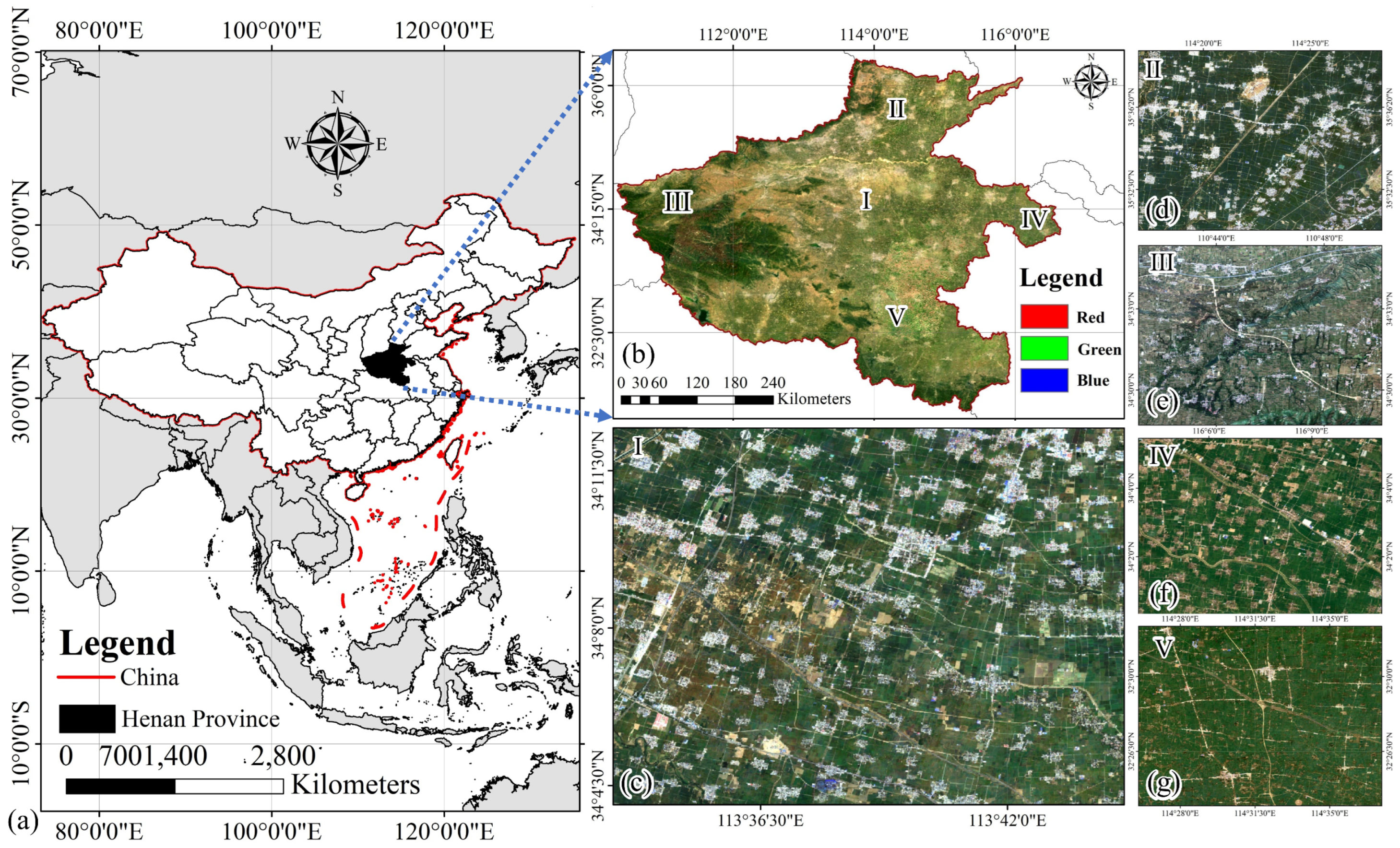
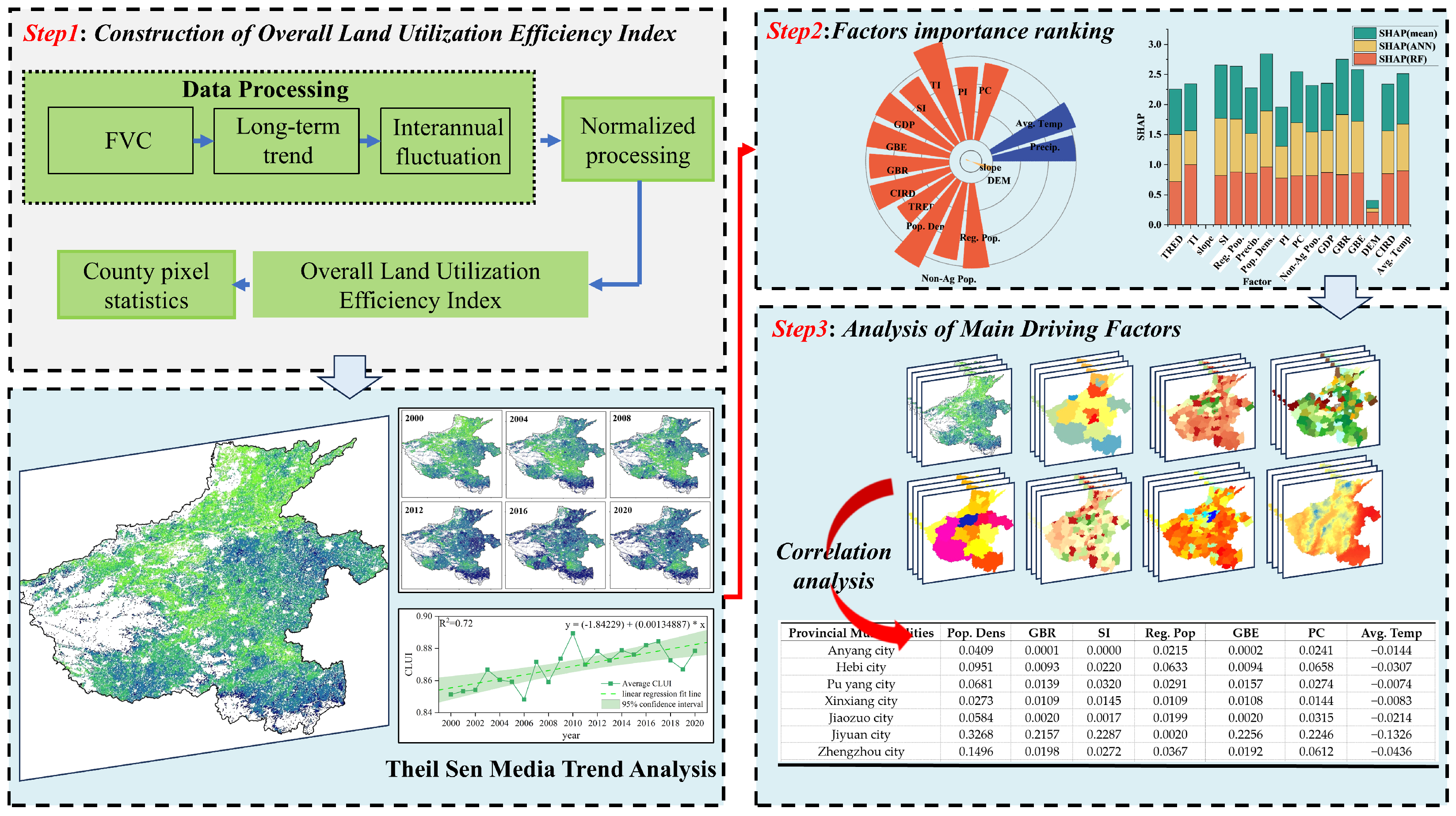

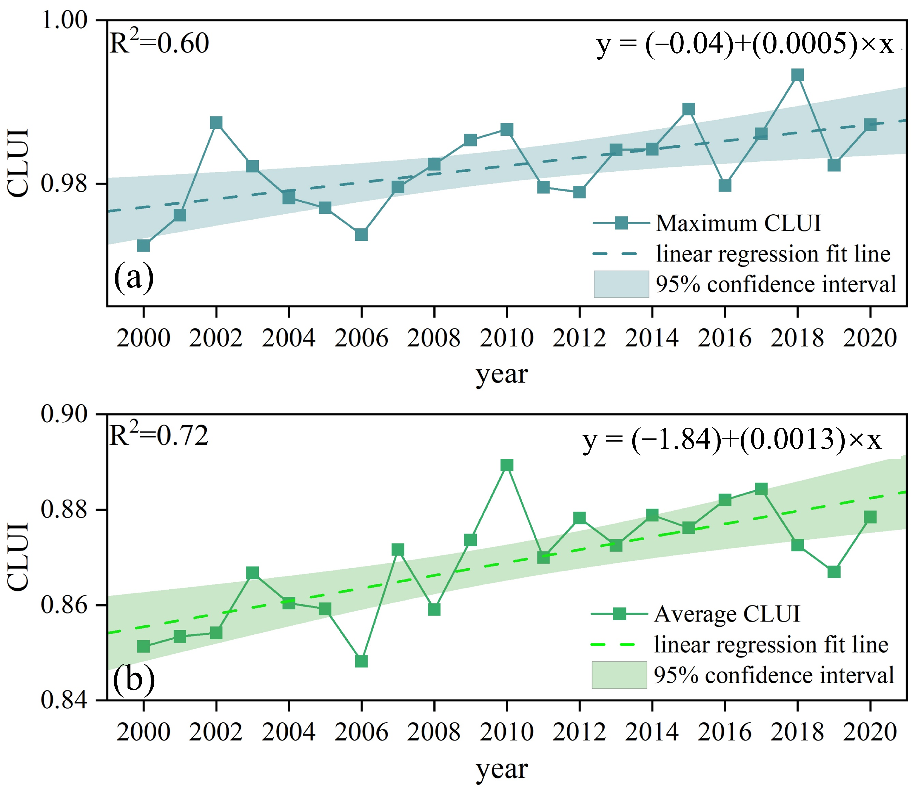
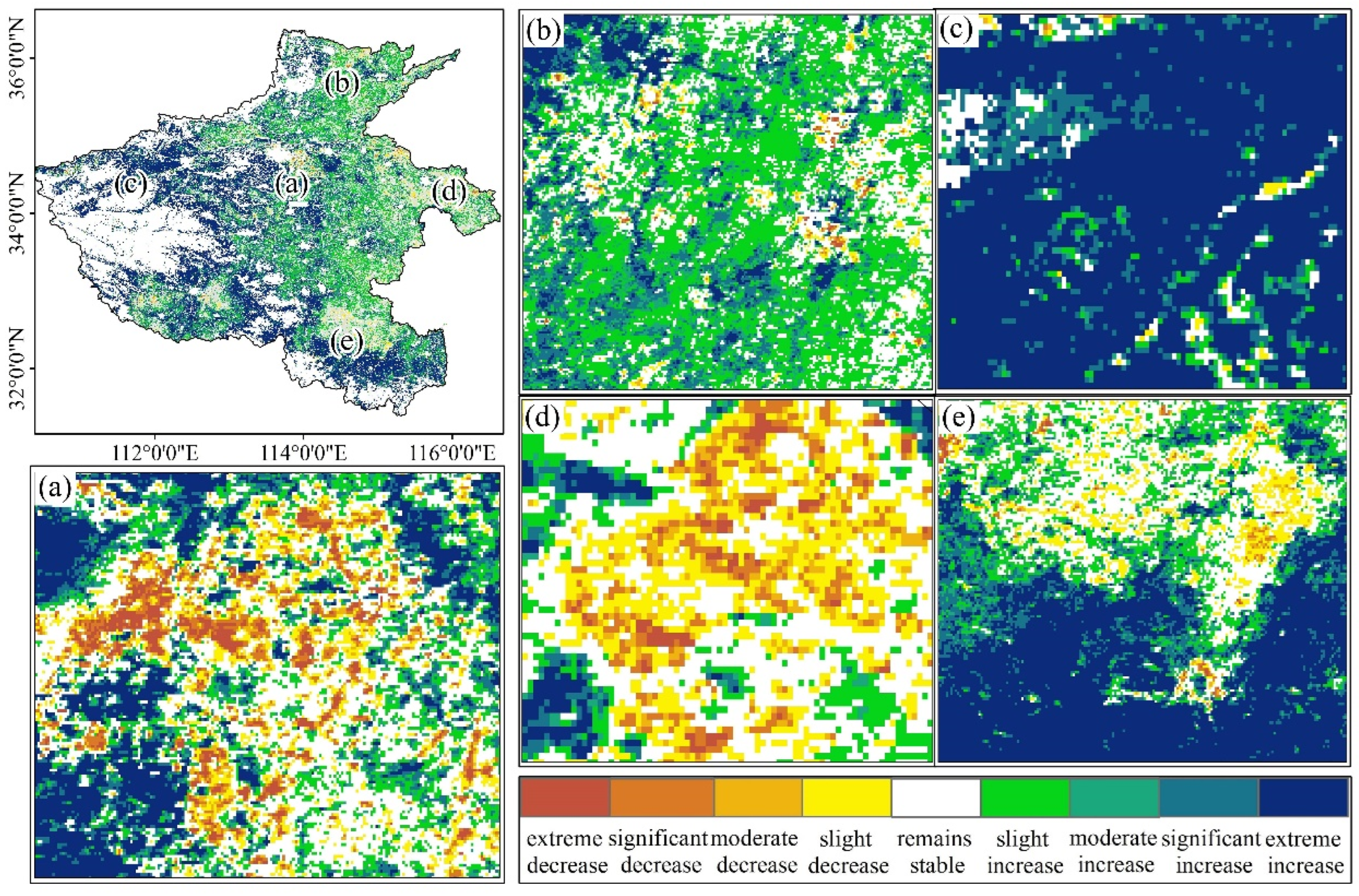
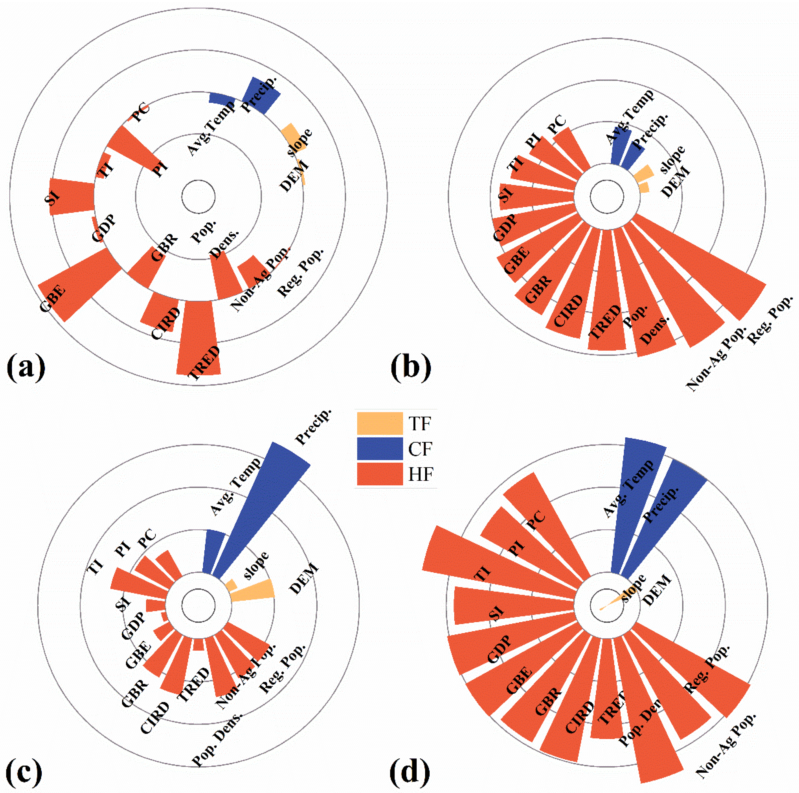
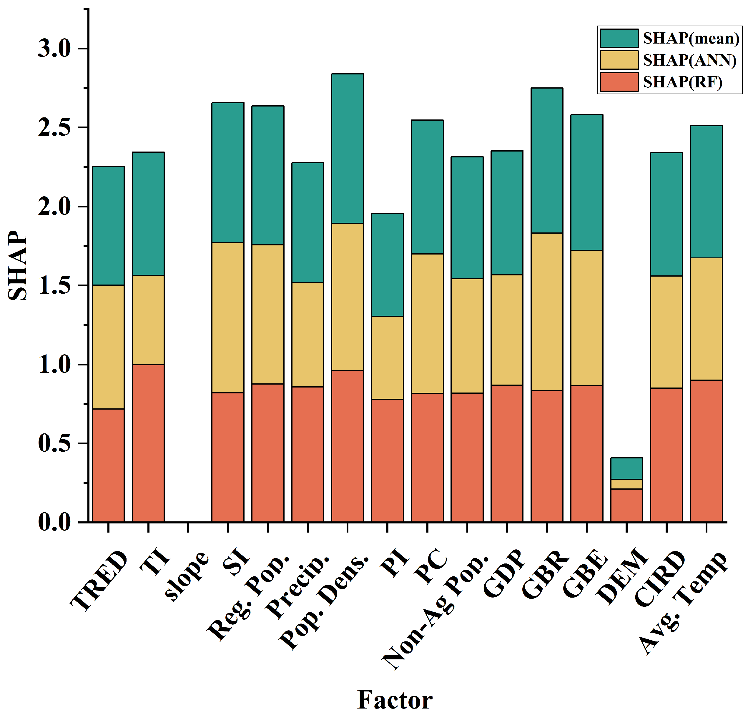
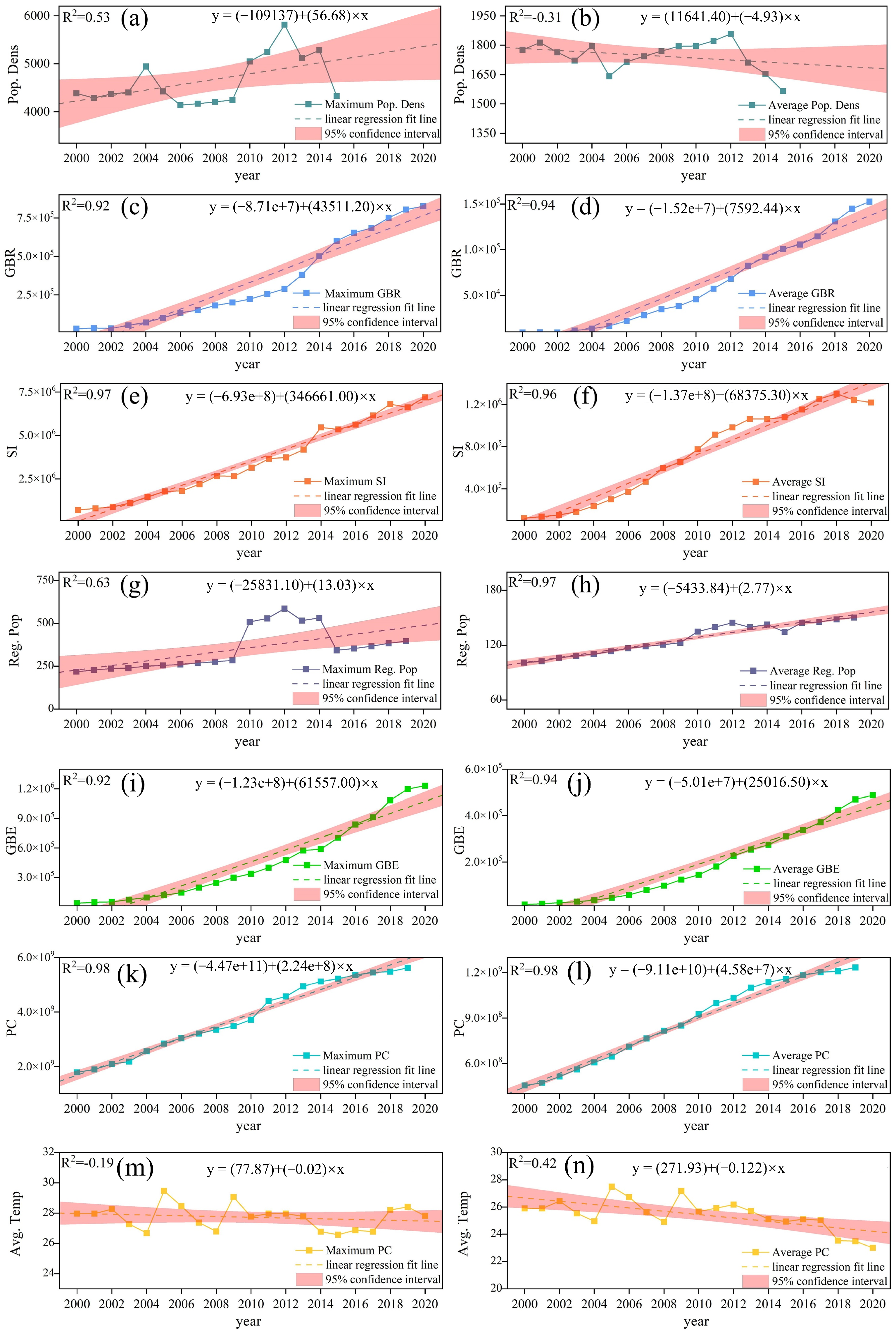

Disclaimer/Publisher’s Note: The statements, opinions and data contained in all publications are solely those of the individual author(s) and contributor(s) and not of MDPI and/or the editor(s). MDPI and/or the editor(s) disclaim responsibility for any injury to people or property resulting from any ideas, methods, instructions or products referred to in the content. |
© 2024 by the authors. Licensee MDPI, Basel, Switzerland. This article is an open access article distributed under the terms and conditions of the Creative Commons Attribution (CC BY) license (https://creativecommons.org/licenses/by/4.0/).