Long-Term Time Series Estimation of Impervious Surface Coverage Rate in Beijing–Tianjin–Hebei Urbanization and Vulnerability Assessment of Ecological Environment Response

Abstract

As urbanization processes are no longer characterized by simple linear expansion but exhibit leaping, edge-sparse, and discontinuous features, spatiotemporally continuous impervious surface coverage data are needed to better characterize urbanization processes. This study utilized GAIA impervious surface binary data and employed spatiotemporal aggregation methods to convert thirty years of 30 m resolution data into 1 km resolution spatiotemporal impervious surface coverage data, constructing a long-term time series annual impervious surface coverage dataset for the Beijing–Tianjin–Hebei region. Based on this dataset, we analyzed urban expansion processes and landscape pattern indices in the Beijing–Tianjin–Hebei region, exploring the spatiotemporal response relationships of ecological environment changes. Results revealed that the impervious surface area increased dramatically from 7579.3 km² in 1985 to 37,484.0 km² in 2020, representing a year-on-year growth of 88.5%. Urban expansion rates showed two distinct peaks: 800 km²/year around 1990 and approximately 1700 km²/year during 2010–2015. In high-density urbanized areas with impervious surfaces, the average forest area significantly increased from approximately 2500 km² to 7000 km² during 1985–2005 before rapidly declining, grassland patch fragmentation intensified, while in low-density areas, grassland area showed fluctuating decline with poor ecosystem stability. Furthermore, by incorporating natural and social factors such as Fractional Vegetation Coverage (FVC), Habitat Quality Index (HQI), Land Surface Temperature (LST), slope, and population density, we assessed the vulnerability of urbanization development in the Beijing–Tianjin–Hebei region. Results showed that high vulnerability areas (EVI > 0.5) in the Beijing–Tianjin core region continue to expand, while the proportion of low vulnerability areas (EVI < 0.25) in the northern mountainous regions decreased by 4.2% in 2020 compared to 2005. This study provides scientific support for the sustainable development of the Beijing–Tianjin–Hebei urban agglomeration, suggesting location-specific and differentiated regulation of urbanization processes to reduce ecological risks.

1. Introduction

As urbanization accelerates globally, with approximately 68% of the population expected to live in urban areas by 2050 [1], understanding the complex relationship between urban expansion and ecological vulnerability has become critical. Urban expansion leads to habitat loss [2], reduced carbon storage, and decreased regional climate regulation capacity [3], particularly in developing countries experiencing rapid growth.

Impervious surfaces are ground areas where water cannot penetrate, such as rooftops, roads, parking lots, and sidewalks [4]. In recent years, they have been widely applied in monitoring and assessment studies of urbanization processes [5], involving mapping and estimating impervious surface area using remote sensing data [6,7], and further used to study long-term dynamic changes in urban expansion [8]. There are now many mature impervious surface data products available, such as artificial impervious surfaces mapped at 250–500 m resolution using Moderate Resolution Imaging Spectroradiometer (MODIS) data [9]; 30 m resolution GAIA (Global Artificial Impervious Area) data generated based on Landsat satellite imagery and auxiliary data [10,11]; and 100 m resolution GISA (Global Impervious Surface Area) data generated by fusing multi-source data [12].

Specifically, GAIA constructs long-term remote sensing index features (such as NDVI, NDBI, MNDWI) by analyzing Landsat satellite imagery (30 m resolution), combined with machine learning methods such as random forest for pixel-level classification judgment; based on the annual impervious status, temporal consistency judgment and threshold setting are further applied to form the final binary product. Grid values of 1 indicate that the pixel is identified as an impervious surface in that year and thereafter, while values of 0 indicate a non-impervious surface [10]. This method has good timeliness and consistency at the global scale, basically conforming to the urbanization process assumption that impervious surfaces grow from none to existence, continuously increase, and are irreversible, and is therefore widely adopted in urban expansion identification and land use change analysis. However, the problem is that existing binary approaches fail to capture urbanization intensity gradients, particularly in areas with sparse development or discontinuous expansion patterns common in contemporary urban growth [13] and cannot reveal the actual proportion of impervious coverage within pixels.

To address this limitation, we constructed Impervious Surface Coverage (ISC) data generated from multi-temporal remote sensing imagery. This data spatially aggregates the 30 m resolution binary impervious surface products provided by GAIA, calculating the proportion of impervious pixels within each 1 km grid to obtain continuous impervious surface proportion data with sub-pixel scale continuity. Compared to traditional binary classification results, this method can more accurately reflect the degree of imperviousness within pixels, demonstrating higher expressive capability and application value in urban impervious intensity assessment, expansion process characterization, and spatial heterogeneity analysis. In contrast, ISC provides a more continuous and refined urban expansion monitoring method, particularly suitable for revealing dynamic processes such as early sparse development and building land density gradient changes [14]. It has good comparability and scalability, suitable for urbanization dynamic monitoring at multiple temporal and spatial scales [15].

Urban expansion impacts on ecosystems are complex and spatially heterogeneous [16], requiring integrated assessment frameworks that capture both urbanization intensity and ecological response patterns [17]. Current ecological vulnerability assessments often rely on subjective weighting schemes [18,19] and fail to establish quantitative relationships between urbanization intensity gradients and ecosystem responses. We address this by developing an Ecological Vulnerability Index (EVI) [20] that integrates natural factors with anthropogenic pressures. Using Genetic Projection Pursuit modeling, we eliminate subjective weighting bias while establishing quantitative ISC–EVI relationships across different urbanization intensity zones.

This study aims to construct a long-term ISC dataset for the Beijing–Tianjin–Hebei region through spatial aggregation methods and by analyzing urban expansion processes and ecological vulnerability patterns, as well as establishing quantitative relationships between urbanization intensity and ecosystem responses to provide scientific support for sustainable regional development strategies. The technical path and analytical framework proposed in this study have multi-dimensional scientific support value for urban ecological security monitoring and spatial regulation in the Beijing–Tianjin–Hebei region. For the ecological vulnerability early warning of high-density urban agglomerations, its core lies in establishing an associated analysis paradigm of “impervious surface dynamics—multi-factor ecological response”: first, converting 30 m resolution impervious surface binary data into 1 km resolution Impervious Surface Coverage (ISC) data through spatial aggregation methods, which solves the scale matching problem between micro data and macro analysis; second, introducing the projection pursuit model to calculate the weights of ecological sensitive factors, avoiding the deviation caused by subjective weighting and improving the objectivity of evaluation results; finally, based on the coupling characteristic analysis of key time nodes, it can capture the evolution law of ecological vulnerability in different development stages. This complete process can be directly transferred to other high-density urban agglomerations such as the Yangtze River Delta and the Pearl River Delta, providing standardized tools for analyzing the urbanization ecological effects in similar regions and establishing a normalized ecological vulnerability early warning mechanism.

2. Materials and Methods

2.1. Study Area

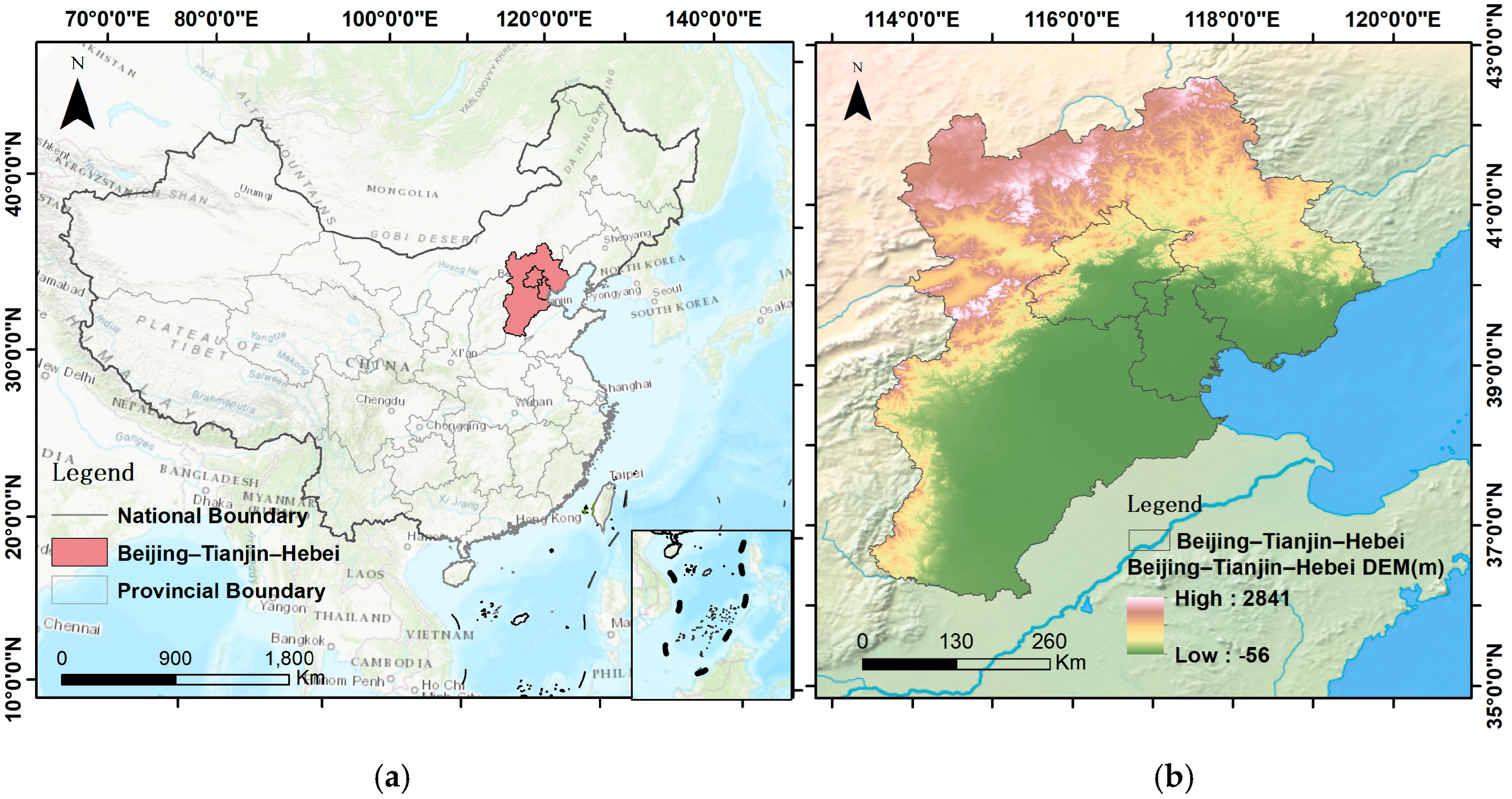
The Beijing–Tianjin–Hebei region (Figure 1) is located in the northern part of the North China Plain, with geographical coordinates of 113°04′–119°53′ E and 36°01′–42°37′ N. It includes two municipalities directly under the central government (Beijing and Tianjin) and 11 prefecture-level cities in Hebei Province (Shijiazhuang, Baoding, Tangshan, Langfang, Handan, Xingtai, Cangzhou, Qinhuangdao, Hengshui, Zhangjiakou, and Chengde), with a total area of approximately 216,000 square kilometers, accounting for 2.3% of the national territory. The Beijing–Tianjin–Hebei region is predominantly plains, with mountains and plateaus. The Yanshan and Taihang mountain ranges surround the northwest, the southeast is the North China Plain, and the east borders the Bohai Sea. It has a temperate monsoon climate with four distinct seasons, annual average precipitation of 400–800 mm concentrated in summer, and is prone to droughts and floods.

The Beijing–Tianjin–Hebei region has a total population of approximately 110 million (2020), with a GDP accounting for about 10% of the national total, making it the economic core area of northern China. The Beijing–Tianjin–Hebei coordinated development strategy was elevated to a national strategy in 2014, with the core objective of relieving Beijing of non-capital functions and promoting industrial, transportation, and ecological integration among the three regions. Beijing serves as the national political, cultural, international exchange, and technological innovation center, focusing on “high-precision and advanced” industries, with the tertiary industry accounting for over 80%. Tianjin is the northern shipping center, characterized by advanced manufacturing and port economy, primarily developing high-end manufacturing and R&D. Hebei is a major industrial and agricultural province with a high proportion of traditional industries such as steel and building materials, undertaking manufacturing industries from Beijing and Tianjin while upgrading traditional industries.

The BTH region was selected for this study due to its significance as a representative case of 21st-century mega-regional urbanization. Covering 216,000 km², BTH exemplifies the scale and complexity of contemporary urban agglomerations that will define global urbanization patterns through 2050. The region’s increase in impervious surface area over our 35-year study period represents one of the most dramatic urban transformations globally, making it an ideal laboratory for testing our ISC methodology and vulnerability assessment framework. Furthermore, the BTH polycentric development pattern, diverse environmental gradients (from megacity cores to pristine mountains), and unique policy context (coordinated regional development strategy) provide insights directly applicable to other rapidly urbanizing mega-regions worldwide.

2.2. Dataset

ISC data utilizes the already mature Global Artificial Impervious Area (GAIA) data for impervious surface coverage mapping. Subsequent ecological vulnerability analysis employs Fractional Vegetation Coverage (FVC) as a proxy indicator for vegetation growth and Land Surface Temperature (LST) as an indicator of climate change, both of which are derived from MODIS satellite data. Specifically, LST data were obtained from the MOD11A1 Version 6 product, which provides daily observations at a spatial resolution of 1 km. We utilized the daytime LST (LST_Day_1 km) values in this study. All data processing was conducted on the Google Earth Engine (GEE) platform, which facilitates large-scale time series analysis and automatic cloud masking. By incorporating all available daily observations throughout each year and computing their annual average, we ensured both the temporal representativeness and robustness of the LST values used in our analysis. Using elevation data from the L-band Phased Array Synthetic Aperture Radar (PALSAR) data of the Advanced Land Observing Satellite (ALOS), elevation, topographic relief, and slope information are extracted. Land use data comes from CLCD data products with a spatial resolution of 30 m from 1985 to 2023, derived from over 335,000 Landsat images on the Google Earth Engine platform. A random forest classifier was trained using samples from the Chinese Land Use Dataset and visually interpreted points. A post-processing step ensured spatial-temporal consistency. The dataset achieved an overall accuracy of 79.31%, averaged across all years based on 5463 validation samples, and outperformed other global land cover products such as MCD12Q1, ESA–CCI, and GlobeLand30.

Population data is derived from gridded population data with a resolution of 1 km. To maintain consistency with all data, we resampled all raster data to 1000 m resolution using the nearest neighbor method. All datasets used are summarized in

Table 1. The details of the used data.

Data Name	Description	Attributes	Usage
Global Artificial Impervious Area (GAIA)	Mapped global urban impervious surface data (1985–2020) as annual maps. Through spatial interpolation and exclusion–inclusion algorithms to achieve rapid annual mapping of impervious surfaces, which can reasonably reflect the spatiotemporal changes in impervious surface sequences.	30 m	Impervious Surface Coverage (ISC) construction
Land Use Data	CLCD data products from 1985 to 2023 are derived from Landsat-based Chinese annual land use products. The dataset achieved an overall accuracy of 79.31%, averaged across all years based on 5463 validation samples.	30 m	Calculate HQI Calculate the landscape index
MOD11A1 V6	Based on Google Earth Engine, the MODIS-provided Quality Control (QC) bands are applied to filter out low-quality pixels affected by clouds, view angle anomalies, and sensor issues.	1000 m	Calculate FVC and LST
DEM	NASA global 30 m SRTM elevation DEM data	30 m	Calculate the slope
Population Data	LandScan dataset developed by Oak Ridge National Laboratory (ORNL), US Department of Energy	1000 m	Calculate the population density

.

2.3. Methods

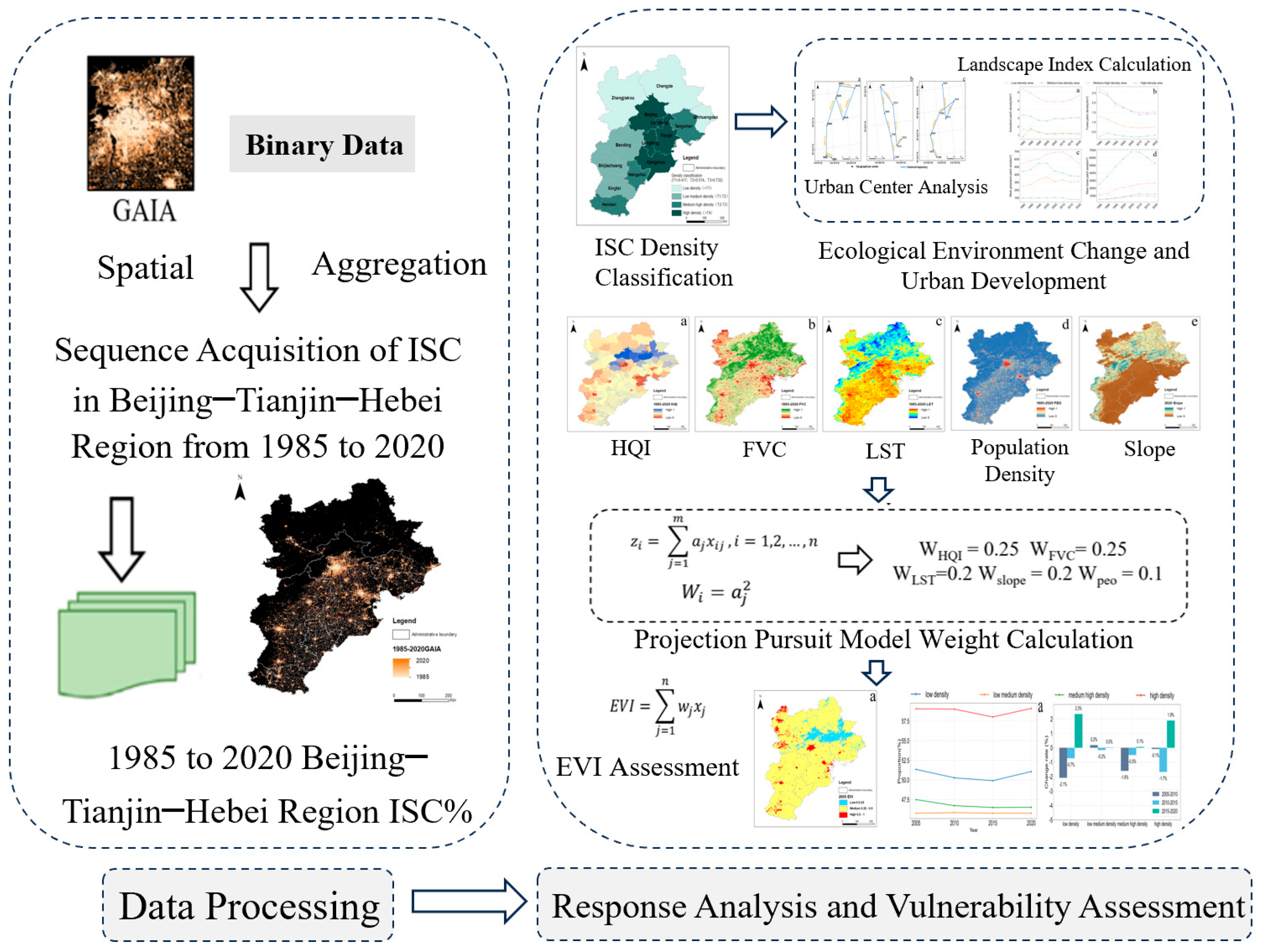
In the data processing stage of this study, spatial aggregation processing was applied to the 30 m resolution GAIA binary data, converting it into coverage proportion data in 1 km grid units. The specific methodology is as follows (Figure 2): First, in the GAIA binary data, “1” represents impervious surface and “0” represents non-impervious surface. We used a sliding window with 1000 m sides to aggregate the original raster, counting the number of pixels with a value of 1 within each 1 km grid and dividing by the total number of pixels contained in that grid, thereby obtaining the coverage proportion of that land type within the 1 km grid (value range 0~1). Additionally, to ensure the accuracy of aggregation results, mask processing was applied to invalid values or edge areas in the original data before processing to avoid interference with statistical results. The final output of 1 km resolution raster data can better reflect the spatial distribution density of target land types at the macro scale, providing fundamental data support for regional-scale land use analysis and modeling. In the impact analysis and vulnerability assessment stage, ecological sensitivity factors such as HQI, FVC, LST, population density, and slope are comprehensively considered to construct an ecological environment change weight factor system, and based on weighted calculations, the Ecological Vulnerability Index (EVI) is computed to assess the impact of urban expansion on ecosystems and regional vulnerability patterns.

2.3.1. Impervious Surface Coverage (ISC) Construction Method

To construct an Impervious Surface Coverage (ISC) dataset with temporal continuity and sub-pixel expression capability, this study selected the 30 m resolution annual binary impervious surface products (1985–2020) provided by GAIA (Global Artificial Impervious Area), where pixel values of 1 represent impervious surfaces and 0 represents non-impervious surfaces. The GAIA dataset demonstrates high accuracy with overall accuracies ranging from 89% to 97% across validation years, with a mean overall accuracy higher than 90% globally and 89% specifically in arid regions using improved algorithms [10]. Considering the low-density development characteristics in urban expansion processes and macro-scale analysis requirements, spatial aggregation methods were employed to convert these into 1 km resolution proportional impervious data. The 1 km resolution was specifically chosen to maintain spatial consistency with other variables in our EVI assessment framework (MODIS-derived FVC and LST data, population density data), while providing an optimal balance between capturing regional urbanization patterns and computational efficiency for the 35-year time series analysis across the 216,000 km² study area. Using 33 × 33 pixels (corresponding to approximately 1 km × 1 km) as aggregation units, the number of impervious pixels with values of 1 within each unit was counted and divided by the total number of pixels to calculate the impervious surface proportion within that 1 km pixel. While this aggregation process inevitably smooths fine-scale heterogeneity and may underestimate urban fragmentation in areas with highly dispersed settlement patterns, it preserves the essential spatial gradients needed for regional-scale urbanization analysis and policy-relevant applications. The high accuracy of the source GAIA data (>90% mean overall accuracy) ensures the reliability of our spatially aggregated ISC dataset. All annual data were processed in the same manner, ultimately generating continuous ISC proportion data sequences from 1985 to 2020. This ISC dataset provides high-resolution, long-term temporal spatial support for subsequent urbanization intensity identification, spatial pattern evolution analysis, and ecological vulnerability assessment, with good regional applicability and explanatory power.

2.3.2. ISC Density Classification Method

Using ISC pixel proportion data, the ISC area of each city in the Beijing–Tianjin–Hebei region was extracted by city level and divided by its administrative area to obtain the ISC density value (ISD) for each city. Since the resulting ISC density values are relatively small, subsequent normalization operations were performed to enhance data comparability and better reflect regional differences. The formula is as follows:

$$T= {\displaystyle \frac{ISD-{ISD}_{min}}{{ISD}_{max}-{ISD}_{min}}}$$

where $T$ is the normalized ISC density value of the image pixel, with values ranging from 0 to 1. The larger the value, the higher the corresponding ISC density; ${ISD}_{max}$ and ${ISD}_{min}$ represent the maximum and minimum values of the study ISC density, respectively.

Traditional methods (such as equal interval division) may be affected by extreme values. To objectively classify ISC density into grades, the mean-standard deviation method is used for density segmentation. The mean-standard deviation method is based on data distribution characteristics and can more adaptively distinguish high, medium, and low density areas. The density segmentation results of different regions are paired to facilitate analysis of spatial differentiation. The density segmentation formula is as follows:

$$T=A\pm X·SD$$

where $T$ is the ISC density classification threshold; $A$ is the average ISC density of the study area; $X$ is the standard deviation multiplier; and $SD$ is the standard deviation of ISC density in the study area.

According to

Table 2. Normalized ISC density classification standards for the study area.

$T\le -0.5SD$	$-0.5SD\le T\le SD$	$SD\le T\le 0.5SD$	$T\ge 0.5SD$
Low-density area	Medium-low density area	Medium-high density area	High-density area

, the ISC density is classified to obtain Figure 3. This graded density map reflects to a certain extent the differentiated urbanization development in different regions of Beijing–Tianjin–Hebei. High-density areas are concentrated in the developed cities in the eastern part of Beijing–Tianjin–Hebei, centered on Beijing and Tianjin, and include Langfang and Cangzhou; medium-low density areas are concentrated in the western part of Beijing–Tianjin–Hebei, and low-density areas are concentrated in the mountainous areas in the northern part of Beijing–Tianjin–Hebei.

2.3.3. Urban Expansion and Center Shift Analysis

Impervious surfaces refer to surfaces covered by impervious materials, typically including surfaces with poor permeability such as rooftops, parking lots, and roads, which are the most prominent characteristics of urbanization [21]. In many studies, cities are defined as an impervious surface area. Studying the dynamic changes and expansion of impervious surfaces can reflect the urbanization process of a region to a certain extent. We use impervious surface expansion speed (ES) to represent the expansion of impervious surfaces within different study periods. The ES index calculation formula is as follows:

$$\mathit{E}\mathit{S}={\displaystyle \frac{{\mathit{S}}_{\mathit{e}\mathit{n}\mathit{d}}-{\mathit{S}}_{\mathit{s}\mathit{t}\mathit{a}\mathit{r}\mathit{t}}}{\mathit{D}}}$$

where ${\mathit{S}}_{\mathit{s}\mathit{t}\mathit{a}\mathit{r}\mathit{t}}$ and ${\mathit{S}}_{\mathit{e}\mathit{n}\mathit{d}}$ are the initial and final areas of impervious surfaces, respectively, $\mathit{D}$ is the time interval, and this study selects a time interval of 5 years.

The impervious surface center is an important indicator that can reflect the spatial characteristics and expansion intensity of urban expansion, and is of great significance for understanding the direction of urban expansion [22]. Using GIS spatial analysis functions, we calculate the impervious surface center coordinates and center migration trajectory for six periods from 1990 to 2015 in the study area, with the formula as follows:

$$X_t=\sum _{i=1}^n{A}_i{X}_i/\sum _{i=1}^n{A}_i$$

$$Y_t=\sum _{i=1}^n{A}_i{Y}_i/\sum _{i=1}^n{A}_i$$

where $X_t$ and $Y_t$ represent the centroid coordinates of impervious surfaces in year t; $A_i$ represents the area of impervious surface patch i; $X_i$ and $Y_i$ represent the centroid coordinates of patch $\mathit{i}$, respectively; and n represents the number of impervious surface patches.

To determine the different center directions of urban development at different levels, time series impervious surface images from six periods were used to calculate impervious surface centroids at both overall and local regional scales: (1) 1990, (2) 1995, (3) 2000, (4) 2005, (5) 2010, (6) 2015, (7) 2020. The calculated time series of impervious surface centroids at different levels reflect the concentration trends of impervious surfaces in different periods, and the spatiotemporal dynamics of urban impervious surfaces at different scales reveal the overall and local evolutionary trajectories of urban impervious surfaces.

2.3.4. Spatiotemporal Response Analysis of Ecological Environment Changes

Vegetation area is the most intuitive indicator for measuring ecological quality [23]. This experiment calculated the forest and grassland areas in the study area based on CLCD data, using them as basic indicators for evaluating environmental changes. Landscape indices are used to describe and quantify the structure and configuration of landscape patterns to assess and monitor changes in landscape patterns. This experiment selected two commonly used indicators: Mean Patch Area (AREA_MN) and Patch Density (PD), to reflect the patch area and fragmentation degree of vegetation areas. All landscape indices were calculated using FRAGSTATS 4.2 software by inputting annual land use raster data from CLCD and applying the landscape metrics calculation module with standard configuration settings. The two indicators for forests and grasslands in different ISC density zones were calculated for 1985, 1990, 1995, 2000, 2005, 2010, 2015, and 2020, respectively. By comparing the different changes in grasslands and forests and the landscape pattern changes in different urbanization development areas, the impacts of different degrees of urbanization development on their surrounding ecological environments are revealed.

2.3.5. EVI Assessment

Calculation of EVI Indicators for Assessment

An ecological vulnerability assessment model for the study area was established using temporally aligned datasets for four target years (2005, 2010, 2015, and 2020). For each target year, all input variables were extracted from the corresponding annual datasets to ensure temporal consistency, using genetic projection pursuit and comprehensive evaluation models to assess the ecological vulnerability of the study area. Combined with the environmental characteristics of the study area, five variables were selected to analyze EVI (Figure 4).

For the vegetation environment aspect, we use Fractional Vegetation Coverage (FVC) and Habitat Quality Index (HQI) to characterize the vegetation environment. FVC is commonly defined as the percentage of the vertical projection area of vegetation (including leaves, stems, and branches) to the total area of the statistical region. It is an important parameter for describing surface vegetation coverage and can intuitively reflect the vegetation prosperity within a region, serving as an important indicator of vegetation growth status. In remote sensing, vegetation coverage is typically calculated using the pixel binary method. $\mathit{H}\mathit{Q}\mathit{I}$ displays the ecological environment quality that supports species and persistence. According to the reference of “Technical Standards for Ecological Environment Assessment” and based on standards promulgated by China’s Ministry of Environmental Protection (MEP-2015), $\mathit{H}\mathit{Q}\mathit{I}$ and $\mathit{N}\mathit{D}\mathit{V}\mathit{I}$ can be calculated as Equations (1) and (2):

$$HQI=(0.35A_f+0.25A_g+0.28A_w+0.11A_c+0.04A_i+0.01A_b)/A$$

(1)

$$FVC={\displaystyle \frac{NDVI-{NDVI}_{soil}}{{NDVI}_{veg}-{NDVI}_{soil}}}$$

(2)

where ${\mathit{A}}_{\mathit{f}}$ is forest area, ${\mathit{A}}_{\mathit{g}}$ is grassland area, ${\mathit{A}}_{\mathit{w}}$ is water body area, ${\mathit{A}}_{\mathit{c}}$ is cultivated land area, ${\mathit{A}}_{\mathit{i}}$ is impervious surface area, ${\mathit{A}}_{\mathit{b}}$ is bare land area, and $\mathit{A}$ is total area. When calculating $\mathit{F}\mathit{V}\mathit{C}$, $\mathit{N}\mathit{D}\mathit{V}\mathit{I}$ values with cumulative probabilities of 0.5% and 99.5% are used as ${\mathit{N}\mathit{D}\mathit{V}\mathit{I}}_{\mathit{s}\mathit{o}\mathit{i}\mathit{l}}$ and ${\mathit{N}\mathit{D}\mathit{V}\mathit{I}}_{\mathit{v}\mathit{e}\mathit{g}}$, respectively, and $\mathit{N}\mathit{D}\mathit{V}\mathit{I}$ values outside this range are considered as pure soil and pure vegetation. MODIS data is used to calculate vegetation coverage for each vegetation area.

Calculation and Classification of Ecological Vulnerability Index

The projection pursuit model is used to find the optimal projection direction vector by constructing projection indicators, and then calculate sample projection eigenvalues from the optimal projection direction vector, thereby conducting comprehensive evaluation of ecological vulnerability. Here, a projection pursuit model based on genetic algorithms is used to evaluate EVI, with a detailed introduction to the construction steps of Genetic Projection Pursuit (GPP). The model is as follows: First, samples are normalized because different indicators have different dimensions. To solve the variability of different indicator scales, each indicator set needs to be normalized by applying the equation:

$$x_{ij}=(x_{ij}^{\mathrm{*}}-x_{min,j})/(x_{max,j}-x_{min,j})$$

where ${\mathit{x}}_{\mathit{m}\mathit{a}\mathit{x},\mathit{j}}$ and ${\mathit{x}}_{\mathit{m}\mathit{i}\mathit{n},\mathit{j}}$ are the maximum and minimum values of the $\mathit{j}$-th indicator in the sample set, respectively, and ${\mathit{x}}_{\mathit{i}\mathit{j}}$ is the normalized indicator value of the sample set.

Subsequently, the projection index function is constructed. Under the execution of projection direction $a_T$ = (a₁, a₂, …, a_m), the m-dimensional data {${\mathrm{x}}_{\mathrm{i}\mathrm{j}}$|j = 1, 2, …, m} for $\mathit{i}$ = 1, 2, …, n can be processed into a one-dimensional value ${\mathit{z}}_{\mathit{i}}$ through the following formula:

$$z_i=\sum _{j=1}^m{a}_j{x}_{ij},i=\mathrm{1,2},\dots ,n$$

The distribution characteristics of projection values ${\mathit{z}}_{\mathit{i}}$ are required to be as follows: local projection points may be concentrated, while overall projection points may be dispersed. Therefore, we construct the projection index function as ${\mathit{Q}}_{\mathit{a}}={\mathit{S}}_{\mathit{z}}{\mathit{D}}_{\mathit{z}}$, where S_Z is the standard deviation of ${\mathit{Z}}_{\mathit{i}}$, and ${\mathit{D}}_{\mathit{z}}$ is the local density of ${\mathit{Z}}_{\mathit{i}}$.

$$S_z=\sqrt{{\displaystyle \frac{\sum _{i=1}^n{(Z_i-E\left(Z_i\right))}^2}{n-1}}}$$

$$D_z=\sum _i^n\sum _k^n\left(R-r_{ik}\right)·u(R-r_{ik})$$

where $\mathit{E}\left({\mathit{Z}}_{\mathit{i}}\right)$ is the mean value of the sequence {$Z_i$|j = 1, 2, …, n}; $\mathit{R}$ is the radius of the window with local density; ${\mathit{r}}_{\mathit{i}\mathit{k}}$ represents the distance between sample projection values, where $r_{ik}$ = |$Z_i$ − $Z_k$| u ($R-r_{ik}$) is the unit step function, when $\mathit{R}$ ≥ ${\mathit{r}}_{\mathit{i}\mathit{k}}$, the function value is 1, otherwise it is 0. Subsequently, we optimize the window radius $\mathit{R}$, providing the function for optimizing the local density window radius $\mathit{R}$, evaluating multiple $\mathit{R}$ values to find the optimal $\mathit{R}$ value that produces the highest projection index $\mathit{Q}$, while considering the balance of weights, and finally obtaining the optimal projection direction vector ${\mathit{a}}_{\mathit{j}}$ through weighted standard deviation evaluation in its optimal solution.

In this study, the synthetic information reflecting each characteristic indicator can be calculated based on the optimal direction vector ${\mathit{a}}_{\mathit{j}}$, and $\mathit{E}\mathit{V}\mathit{I}$ can be evaluated based on the variance level of the synthetic information. Therefore, indicator standardized values and standardized weights are used to calculate $\mathit{E}\mathit{V}\mathit{I}$, with the equation as follows:

$$W_i=a_j^2$$

$$EVI=\sum _{j=1}^n{w}_j{x}_j$$

Since the calculated results are mostly concentrated in the middle range, the quantitative evaluation results of ecological vulnerability in the study area are classified into three categories using the natural breaks (Jenks) classification method in ArcMap based on the actual $\mathit{E}\mathit{V}\mathit{I}$ values from four study years (2005, 2010, 2015, and 2020). This data-driven approach maximizes the contrast between vulnerability classes and ensures meaningful ecological distinctions: low vulnerability area ($\mathit{E}\mathit{V}\mathit{I}$ < 0.25), moderate vulnerability area (0.25 < $\mathit{E}\mathit{V}\mathit{I}$ < 0.50), and high vulnerability area ($\mathit{E}\mathit{V}\mathit{I}$ > 0.50).

3. Results

3.1. Spatiotemporal Evolution Analysis of Urbanization in Beijing–Tianjin–Hebei

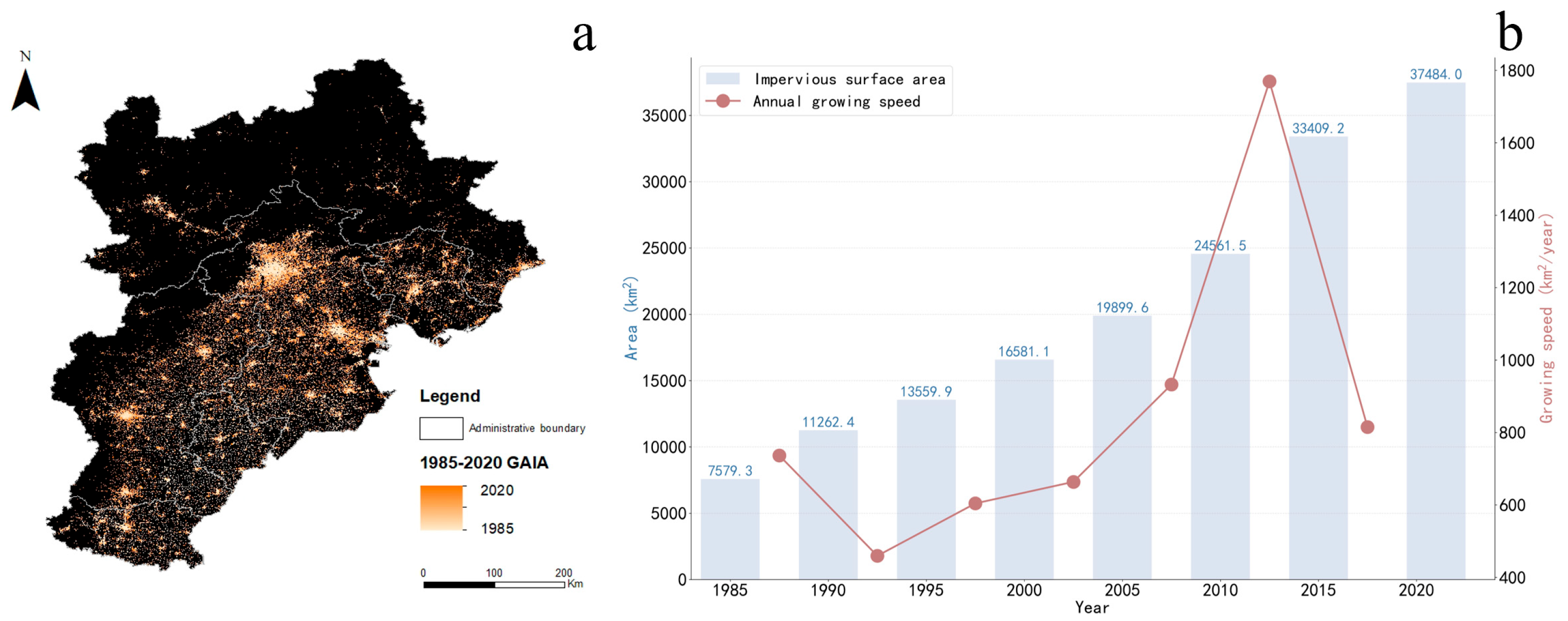
In Figure 5a, which displays the cumulative overlay of annual impervious surface data from 1985 to 2020, it can be clearly observed that the urban core areas of Beijing and Tianjin, as well as the urban agglomeration in southeastern Hebei, show obvious outward expansion trends. The color gradient from light to dark orange illustrates the temporal sequence of impervious surface development over the 35-year period. Specifically, Beijing, as the core city of the Beijing–Tianjin–Hebei urban agglomeration, demonstrated the highest mean annual expansion rate of 115.17 km²/year and has simultaneously driven the coordinated development of surrounding cities such as Langfang (90.63 km²/year) and Baoding (108.56 km²/year). In contrast, Chengde (21.44 km²/year) and Zhangjiakou (36.68 km²/year) in northern Hebei have experienced relatively slow urbanization due to factors such as topographical constraints and ecological protection policies, with their main development period concentrated after 2000.

The urbanization process in the Beijing–Tianjin–Hebei region has undergone a transformation from rapid expansion to gradual deceleration over the past 30 years. Although the built-up area continues to grow, the expansion speed has significantly slowed in recent years. According to calculations, the impervious surface area in the Beijing–Tianjin–Hebei region increased from 7579.3 km² in 1985 to 37,484.0 km² in 2020, representing a total growth of 394.5% over the 35-year period, with an average annual increase of 854.4 km²/year (Figure 5b). In terms of growth rate, the impervious surface growth in the Beijing–Tianjin–Hebei region from 1985 to 2000 showed a pattern of initial decline, followed by increase, then decrease again. The expansion rate experienced a dramatic surge around 1990, with a growth rate of 800 km²/year; subsequently dropping sharply to reach the lowest point; then experiencing rapid growth again around 2010, reaching a peak during 2010–2015 at approximately 1700 km²/year; followed by a declining trend. The overall trend shows that the built-up land area in the Beijing–Tianjin–Hebei region continues to grow and has experienced two rapid expansion phases.

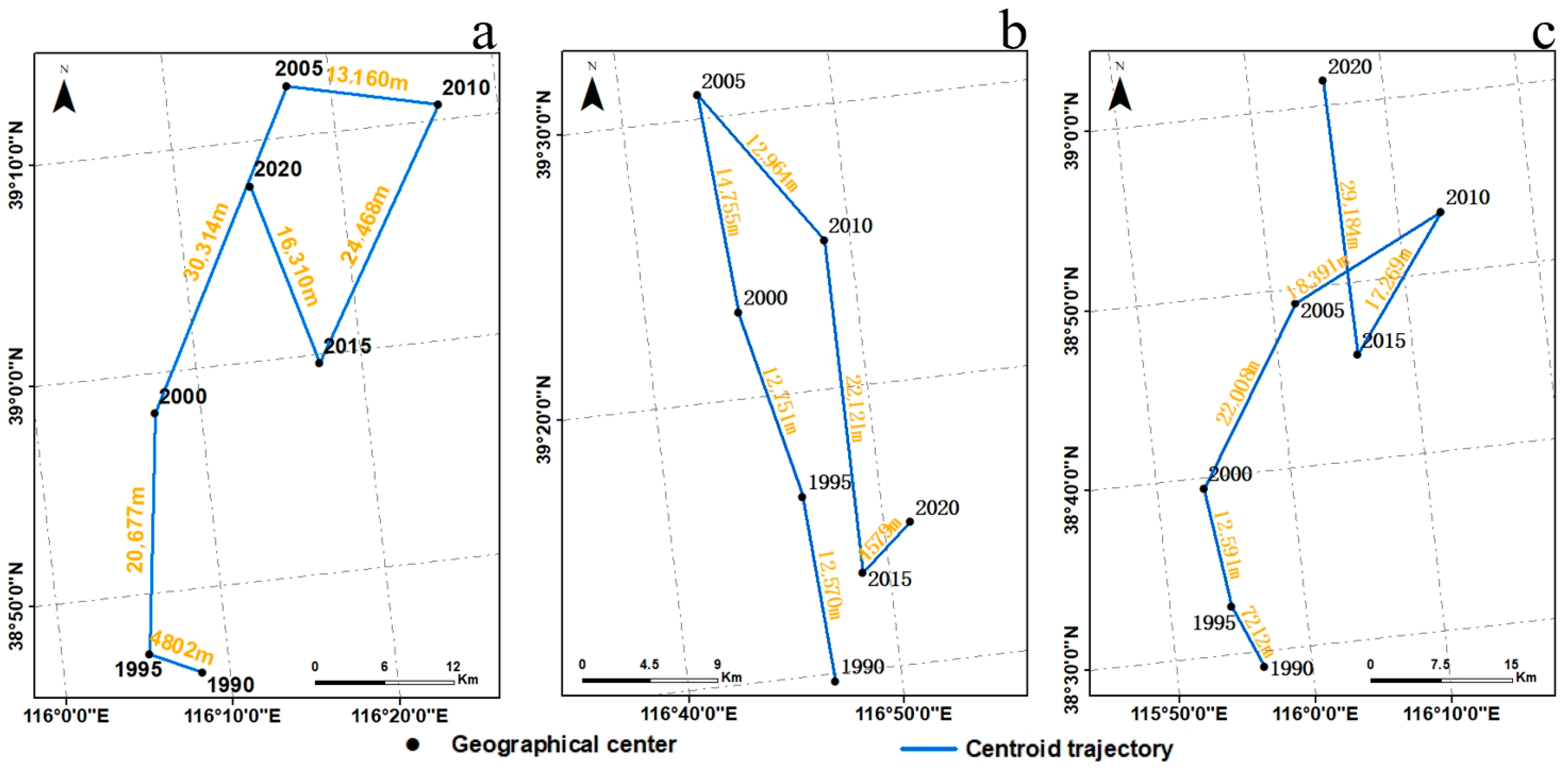
To reveal the centroid changes in urban development in the Beijing–Tianjin–Hebei region, the impervious surface centroid at the regional scale was estimated using six-period ISC images. The weighted average center of impervious surfaces at the regional scale and its movement trajectory are shown in Figure 6.

Figure 6a shows that the centroid of the Beijing–Tianjin–Hebei region exhibited a northward-then-southward transfer trend from 1990 to 2015. During 1990–2000, influenced by the early urbanization of Beijing and Tianjin, the centroid moved closer to the Beijing–Tianjin corridor. During 2005–2015, the urban centroid moved toward the southeast, reflecting the enhanced economic growth and population agglomeration effects in southeastern Hebei. The relatively short centroid movement distance indicates that regional overall development is relatively balanced, but there exists slight spatial imbalance.

By separately analyzing the centroid transfer of high-density ISC areas and Hebei province (Figure 6c), it can be observed that the centroid transfer direction of high-density ISC areas is basically consistent with the overall Beijing–Tianjin–Hebei trend. The relocation of heavy industries such as Shougang in Tangshan and the rapid development of the Caofeidian Industrial Zone in the coastal economic belt have driven industrial transfer toward Hebei. However, Hebei’s centroid did not shift southeast but instead pointed toward northeastern cities such as Tangshan and Qinhuangdao, indicating that the coordinated development of Beijing–Tianjin–Hebei has promoted resource dispersion to Hebei, but within the province, it is still dominated by historical steel industries and geographical advantages of ports. The overall southeastern movement of Beijing–Tianjin–Hebei reflects the supplementary role of southeastern Hebei cities such as Cangzhou and Hengshui, while Hebei’s independent northeastern movement reflects the shift of the province’s economic core from the south to the northeastern coastal areas.

3.2. Spatiotemporal Evolution Analysis of Ecological Environment Vulnerability in Beijing–Tianjin–Hebei

Four periods of data from the years 2005, 2010, 2015, and 2020 were selected, and according to the regional divisions classified by ISC density levels, different weights were assigned to different indicators, ultimately calculating the EVI results for different ISC density regions as shown in Figure 7. Overall, the ecological vulnerability in the Beijing–Tianjin–Hebei region exhibits obvious geographical spatial variability, with EVI levels divided into three categories: low (0–0.25), medium (0.25–0.5), and high (0.5–1). The ecological vulnerability index is higher in urban centers, while it is lower in the mountainous areas of northern Beijing and eastern Hebei, which mainly reflects that the abundant forest resources in the northeastern part of the Beijing–Tianjin–Hebei region can protect their ecological environment at any time. The main changes occur in high-value areas of ecological vulnerability, which are also the most noteworthy regions. The high-value areas of ecological vulnerability in Beijing’s urban center show no obvious changes, while in Tianjin and Tangshan, the high-value areas of ecological vulnerability show obvious expansion trends. The high-value areas of ecological vulnerability in the northwestern Beijing–Tianjin–Hebei region show a reduction trend. The low-value areas of ecological vulnerability gradually decreased from 2005 to 2015, then recovered in 2020.

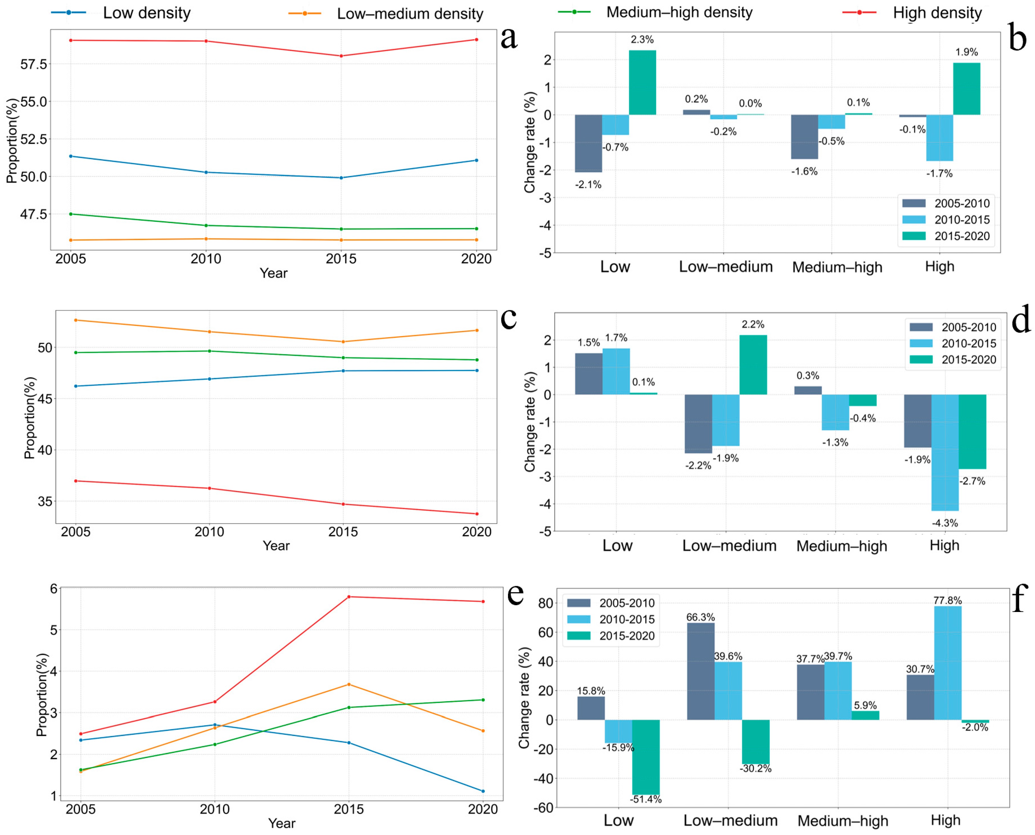
Figure 8 shows the changes in the proportion of high, medium, and low EVI levels in different ISC density level regions and the changes in vulnerability indices for different ISC density levels. The high EVI values in high ISC density areas, namely, urban core areas, have increased significantly, indicating obvious effectiveness of urban greening construction; the vegetation health conditions in low ISC density areas, namely, mountainous or rural areas on the periphery of Beijing–Tianjin–Hebei, have fluctuated in recent years, particularly with a significant decline in high EVI values; the differentiation of EVI values in different density areas is obvious, with vegetation quality improvement in high-density areas while other areas show varying degrees of fluctuation.

In the trend of low EVI value changes in different ISC density areas, high ISC density areas have the highest low EVI values, fluctuating between 58 and 59%, with a slight decline in 2015 but recovering to 59.12% by 2020. Low ISC density areas rank second, fluctuating between 49.91 and 51.35%. Medium-high and medium-low ISC density areas have the lowest EVI values, ranging between 46–47.5% and 45.7–45.8%, respectively (Figure 8a). Notably, both low and high ISC density areas showed positive growth during 2015–2020, at 2.3% and 1.9%, respectively, while they mostly showed negative growth during 2005–2010 and 2010–2015 periods (Figure 8b).

In the trend of medium EVI value changes in different ISC density areas, medium-low ISC density areas have the highest medium EVI values, ranging between 50.55 and 52.66%, followed by medium-high ISC density areas at 48.78–49.64%, then low ISC density areas at 46.21–47.74%, with high ISC density areas being the lowest and showing a continuous declining trend, from 36.97% in 2005 to 33.76% in 2020 (Figure 8c). The medium EVI change rates for different density areas in different periods show the following: medium-low ISC density areas had significant growth of 2.2% during 2015–2020, while high ISC density areas had the most obvious decline of −4.3% during 2010–2015 (Figure 8d).

In the trend of high EVI value changes in different ISC density areas, high ISC density areas showed the most significant growth in high EVI values, rising from 2.49% in 2005 to 5.80% in 2015, with a slight decline to 5.68% in 2020. Medium-high and medium-low ISC density areas also showed overall upward trends, while low ISC density areas peaked at 2.71% in 2010 and then continuously declined to 1.11% in 2020 (Figure 8e). During 2010–2015, high ISC density areas had a growth rate as high as 77.8%, while during 2015–2020, low ISC density and medium-low density areas experienced significant declines of −51.4% and −30.2%, respectively (Figure 8f).

3.3. Impact of Continuous Urbanization Growth on Regional Environment in Beijing–Tianjin–Hebei

Figure 9 reveals the dynamic coupling relationship between urbanization processes and ecological vulnerability. The long-term time series ISC indicators not only effectively depict the spatial expansion pathways of urbanization, but also provide a basis for understanding its impact on ecosystem stability and resilience. Figure 9a shows the changing trends of ecological vulnerability in different ISC density areas (high density and low density) from 2005 to 2020. The results indicate that the EVI mean values in high ISC density areas increased significantly (R² = 0.7047), growing from approximately 0.39 in 2005 to 0.44 in 2015, followed by a slight decline. This trend may reflect that urban center areas, during rapid urbanization processes, have alleviated ecological vulnerability to some extent through artificial greening and ecological engineering measures. The EVI fluctuations in low ISC density areas were smaller, showing an overall slight decline (R² = 0.1077), indicating that as urban peripheries expand outward, the original ecosystems in these areas are gradually being eroded, with ecological vulnerability somewhat intensified.

Statistical hypothesis testing revealed significant differences in EVI values between high and low ISC density areas across all study years (p < 0.001, indicated in Figure 9b), confirming the validity of our density-based classification approach and the distinct ecological vulnerability patterns in different urbanization zones.

Figure 9c further reveals the quantitative relationship between impervious surface expansion and ecological vulnerability changes. The figure divides the ISC increment from 2005 to 2020 into several intervals and statistics the corresponding EVI differences within each interval. The results show that as the magnitude of ISC growth increases, EVI change values tend toward the negative direction, with mean values continuously declining. Significant differences were observed between different ISC increment groups (p < 0.001, Figure 9c), indicating that impervious surface expansion driven by urbanization significantly intensifies ecosystem vulnerability, meaning that the more intense urban development is, the greater the degree of regional ecosystem degradation.

We further studied landscape pattern changes under different ISC density regions. Forests and grasslands are affected differently by urbanization, and the changes in forests and grasslands in regions with different degrees of urbanization also vary. Two indicators reflect the landscape pattern changes in different density regions during China’s urbanization process, showing the changing trends in the quantity and area of grassland and forest patches, particularly the significant increase in average forest area in high-density regions, reflecting the strengthening of urban greening processes. Although the grassland patch density in low-density areas has declined somewhat, it remains the highest, indicating that the natural landscapes in these areas maintain a relatively dispersed pattern. Figure 10 uses two landscape indices, Mean Patch Area (AREA_MN) and Patch Density (PD), to reflect the vegetation patch area and patch fragmentation degree, respectively. Combined with the above-divided ISC density levels from T_1 to T_4, the changes in landscape quality of different urbanization level regions are calculated in the Beijing–Tianjin–Hebei area.

The grassland patch density in low-density regions shows an overall trend of initial decline followed by a small recovery, but remains much higher than other density regions. Medium-low density regions are relatively stable, while medium-high density and high-density regions have lower values with little change (Figure 10a). The forest patch density in all density regions shows an overall declining trend, then tends to stabilize. Low-density and medium-low density regions have higher forest patch density, followed by medium-high density regions, while high-density regions are the lowest (Figure 10b). The average grassland area in low-density regions increased significantly from 1985 to 2010, then declined sharply thereafter. Medium-low density regions peaked in 1995 and then continued to decline. Medium-high density regions show a fluctuating upward trend, while high-density regions maintain relatively low levels (Figure 10c). The average forest area in high-density regions shows the most significant growth, rising from approximately 25 hectares in 1985 to nearly 70 hectares in 2005, followed by some decline. Low-density regions also show a steady upward trend, while the growth in medium-low density and medium-high density regions is relatively small (Figure 10d).

3.4. Development Intensity and Construction Rhythm Reflected by Urban Impervious Surface Evolution

Figure 11 shows, using Beijing as an example, correlation analysis between ISC change values and EVI change values at the grid scale, revealing the spatial coupling relationship between urbanization processes and ecological vulnerability (Figure 11a). By calculating the Pearson correlation coefficients of the change differences between ISC and EVI from 2005 to 2018, positive and negative correlation regions with spatial heterogeneity were obtained. Two typical representative areas were selected for further analysis: the Temple of Heaven park area (correlation coefficient +0.6, p < 0.001) and the Capital Airport area (correlation coefficient −0.5, p < 0.001). Our correlation analysis was conducted using all available grid cells within each study area over the 2005–2020 period, resulting in large sample sizes (n > 1000 for each area) that ensure high statistical power. The former shows a positive correlation, indicating that the increase in impervious surfaces is accompanied by the alleviation of ecological vulnerability; the latter exhibits significant negative correlation, indicating that the increase in urban construction intensity is highly coupled with ecosystem degradation.

ISC is not only a spatial marker of urbanization intensity, but can also reflect the temporal rhythm and spatial pathways of urbanization processes [4]. To further explore the ISC temporal capability in urbanization characterization, Figure 11b and c, respectively show three change dimension layers of ISC within the above two areas: change magnitude, change year, and change duration, to characterize the intensity, timing, and process characteristics of urban construction. The change magnitude layer reflects the cumulative increment of impervious surface coverage proportion in each pixel. In the Capital Airport area, change magnitude values are significantly higher than in the Temple of Heaven area, indicating that it has experienced large-scale land development and hardening processes. The impervious surface increase in the Temple of Heaven area is relatively small, indicating that its surface changes are mainly concentrated in green space restoration and structural adjustment. The change year layer reveals the specific temporal distribution of urbanization activities, showing obvious spatial agglomeration patterns. As shown in the figure, impervious expansion in the airport area mainly occurred between 2008 and 2015, corresponding to the concentrated period of large-scale infrastructure construction, while the Temple of Heaven area shows earlier, scattered change characteristics. The change duration layer records the number of years each pixel experienced in transforming from non-impervious to impervious surface, reflecting the continuity and rhythm of construction activities. The airport area generally shows rapid, short-term (≤3 years) development characteristics, indicating that its urbanization process exhibits explosive characteristics, while the Temple of Heaven area shows longer change duration periods in local pixels, suggesting the existence of multi-stage urban intervention activities, such as green space reconstruction and chronic expansion.

4. Discussion

4.1. Comparison with Other Global Urban Products

To validate the reliability and accuracy of our constructed ISC dataset, we conducted comprehensive comparisons with existing global urban products and assessed potential uncertainties in our methodology across multiple urban agglomerations.

Figure 12 presents the Pearson correlation coefficient distributions between our ISC dataset and the Global Human Settlement Layer (GHSL) data across three major urban agglomerations in China: (a) Beijing–Tianjin–Hebei, (b) Yangtze River Delta, and (c) Pearl River Delta. Due to the GHSL five-year interval data availability, we employed a sampling strategy extracting corresponding years from both datasets to assess correlation coefficients and constructed histograms of these correlations.

The results demonstrate consistently high correlations across all three regions: Beijing–Tianjin–Hebei shows a mean correlation of μ = 0.8218 (σ = 0.1750), Yangtze River Delta achieves μ = 0.8899 (σ = 0.1221), and Pearl River Delta reaches μ = 0.8943 (σ = 0.1171). The progressive improvement in correlation coefficients from north to south may reflect regional differences in urbanization patterns, data quality, or methodological sensitivities. Notably, all three distributions show strong right-skewed patterns with most correlation values exceeding 0.8, confirming the robustness of our ISC methodology across diverse urban contexts.

Figure 13a presents a comprehensive time series comparison of annual impervious surface area trends between our ISC dataset and multiple established global urban products, including ESA–CCI land cover data, Zhou et al.’s urban extent dataset [24], and Global Impervious Surface Area (GISA), over the period 1985–2019. All datasets capture the characteristic rapid urbanization pattern in the Beijing–Tianjin–Hebei region, with consistent identification of the major expansion peaks around 2010–2015. However, subtle differences exist in absolute values, which can be attributed to varying methodological approaches: ESA–CCI employs multi-sensor fusion techniques, Zhou et al.’s dataset relies on nighttime light calibration, while GISA and our ISC use similar Landsat-based approaches [12]. Despite these methodological differences, the overall temporal trends remain remarkably consistent, validating the fundamental urbanization dynamics captured by our dataset.

Given that GISA employs the most similar data acquisition methodology to our ISC approach and provides the most temporally consistent coverage, we conducted an in-depth correlation analysis between these two datasets (Figure 13b). Using 700 randomly distributed sampling points across the study area from 1985 to 2019, the analysis reveals a strong positive correlation (R² = 0.804, p < 0.001), demonstrating high consistency between our ISC estimates and the established GISA product. The linear relationship indicates that our ISC values are slightly conservative compared to GISA, which can be attributed to our spatial aggregation approach that tends to smooth extreme values within 1 km grid cells while maintaining the overall spatial and temporal patterns.

4.2. Contributions and Limitations of ISC Data Construction

Our ISC construction methodology offers several significant contributions to urban monitoring and analysis. First, the spatial aggregation approach from 30 m binary GAIA data to 1 km continuous coverage data addresses a critical gap in urbanization monitoring. Traditional binary classification approaches, while effective for identifying the presence or absence of impervious surfaces, fail to capture the subtle gradations of urban development intensity, particularly in peri-urban areas where sparse development patterns are common [25]. Our ISC method provides sub-pixel continuity that better reflects the heterogeneous nature of urbanization processes, especially valuable for characterizing low-density development and gradual urban expansion patterns. Also, the temporal continuity maintained throughout the 35-year period (1985–2020) provides unprecedented insights into urbanization dynamics. In contrast to many existing products that rely on discrete time points or have temporal gaps, our annual ISC dataset enables the detection of subtle year-to-year variations in urban expansion rates and intensity changes. This temporal granularity is particularly important for understanding policy impacts, economic cycles, and environmental responses to urbanization.

Despite these contributions, several limitations must be acknowledged. The spatial aggregation process, while providing continuity, inevitably results in some information loss compared to the original 30 m resolution. Small, isolated impervious patches may be averaged out within the 1 km grid, potentially underestimating urban fragmentation in some areas. This smoothing effect may be particularly pronounced in regions with highly dispersed settlement patterns or complex urban morphologies [26].

The dependency on GAIA source data introduces inherited uncertainties. While GAIA demonstrates high overall accuracy (>90%), regional variations in classification performance may propagate through our aggregation process. Cloud contamination, seasonal variations in satellite imagery, and the challenges of distinguishing between different types of impervious surfaces in the source Landsat imagery can introduce localized errors. Additionally, the assumption of irreversible impervious surface growth, while generally valid, may not capture all real-world scenarios. Urban renewal projects, building demolition, or conversion of paved areas back to vegetation can result in decreases in impervious surface coverage that our methodology may not fully represent. This limitation is particularly relevant for mature urban areas undergoing redevelopment or cities implementing green infrastructure initiatives [27].

4.3. Contributions and Limitations of EVI Assessment

The integration of the Genetic Projection Pursuit (GPP) model for weight determination addresses a critical limitation in traditional vulnerability assessments that rely on subjective expert judgment or arbitrary weighting schemes. By optimizing projection directions through genetic algorithms, our approach ensures that indicator weights reflect the actual data structure and relationships, enhancing the objectivity and reproducibility of vulnerability assessments. The multi-dimensional indicator system incorporating both natural (FVC, HQI, LST, slope) and anthropogenic (population density, ISC) factors provides a comprehensive representation of ecological vulnerability drivers. This holistic approach captures the complex interactions between urbanization pressures and environmental responses, offering insights that single-factor analyses would miss. The inclusion of topographic variables (slope) is particularly valuable in the Beijing–Tianjin–Hebei context, where mountainous areas in the north exhibit fundamentally different vulnerability patterns compared to the plain regions [28].The temporal analysis framework linking EVI changes to urbanization intensity gradients reveals dynamic vulnerability patterns that static assessments cannot capture. The classification of areas into different ISC density zones enables the identification of threshold effects and non-linear responses in ecological systems, providing crucial information for understanding when and where urbanization pressures exceed ecosystem resilience capacities.

Several limitations constrain the interpretation and application of our EVI results. The temporal resolution of EVI assessment (5-year intervals from 2005 to 2020) may miss rapid environmental changes or short-term fluctuations that could be ecologically significant [29]. Climate variability, extreme weather events, and sudden policy interventions can cause vulnerability patterns to change more rapidly than our assessment framework can capture [30]. Furthermore, the Habitat Quality Index calculation relies on fixed coefficients derived from national standards that may not adequately reflect local ecological conditions or species-specific habitat requirements in the Beijing–Tianjin–Hebei region. The assumption of linear relationships between land cover types and habitat quality may oversimplify complex ecological processes and species–habitat relationships.

4.4. Implications for Areas with Coexisting Urbanization and Rural Development

Based on our findings, several key policy recommendations emerge for sustainable urban development in the Beijing–Tianjin–Hebei region. First, the identification of high vulnerability expansion areas, particularly around Beijing and Tianjin cores, necessitates the implementation of differentiated urban growth management strategies [31]. High-density areas showing positive EVI trends (such as the Temple of Heaven area) demonstrate that well-planned urban intensification combined with ecological restoration can achieve win-win outcomes [32]. These successful models should be replicated in other high-density areas through policies promoting green infrastructure integration and urban ecological restoration.

Second, the declining ecological quality in low-density areas requires urgent attention to prevent further ecosystem degradation. The 4.2% decrease in low vulnerability areas in northern mountainous regions indicates that current environmental protection measures may be insufficient. Enhanced ecological compensation mechanisms, stricter development controls in ecologically sensitive areas [33], and increased investment in ecosystem restoration are needed to reverse this trend.

Third, the spatial heterogeneity in urbanization–ecology relationships calls for location-specific management approaches rather than uniform regional policies. The contrasting patterns observed between the airport area (negative correlation) and Temple of Heaven area (positive correlation) suggest that urban development impacts depend heavily on local context, existing ecological conditions, and development practices [34]. Policy frameworks should incorporate these spatial variations through zone-specific regulations and incentive structures.

5. Conclusions

This study constructed a long-term time series Impervious Surface Coverage (ISC) dataset for the Beijing–Tianjin–Hebei region from 1985 to 2020 through spatial aggregation of 30 m GAIA data, and analyzed the spatiotemporal response relationship between urbanization and ecological environment changes.

The regional impervious surface area increased dramatically from 7579.3 km² in 1985 to 37,484.0 km² in 2020, representing a total growth of 394.5% over the 35-year period, with expansion rates showing two distinct peaks around 1990 and 2010–2015. Urban centers migrated from the Beijing–Tianjin corridor toward southeastern Hebei, reflecting regional development acceleration. The forest area in high-density regions increased significantly during 1985–2005 before declining, while grassland fragmentation intensified in low-density areas primarily driven by the discontinuous urban expansion pattern characteristic of Chinese urbanization [35], exacerbated by linear infrastructure development and agricultural conversion policies [36]. The Ecological Vulnerability Index assessment revealed expanding high vulnerability areas in Beijing–Tianjin cores, which may be attributable to the concentration of urban development pressures, including population agglomeration [37], urban heat island intensification [38], and insufficient green infrastructure development relative to urbanization pace. Conversely, the 4.2% decline in low-vulnerability mountainous areas results from multiple stressors including climate change impacts on montane ecosystems [39], as well as tourism and infrastructure development pressure. While conservation policies such as ecological protection zones and afforestation programs have been implemented in the Beijing–Tianjin–Hebei region, our findings suggest that these measures may not be fully offsetting the combined pressures of climate change and development activities in peripheral areas. The declining trend indicates a need for enhanced conservation strategies and stricter implementation of environmental protection policies in low-density regions.

ISC and EVI relationships showed significant spatial heterogeneity: positive correlations in areas like the Temple of Heaven (indicating successful urban renewal with ecological improvement) contrasted with negative correlations around Capital Airport (reflecting ecological degradation from rapid expansion). These findings highlight urgent needs for location-specific urban planning strategies that balance development with ecological protection.

Several key research directions emerge from this study that warrant further investigation. First, the temporal resolution of vulnerability assessment could be enhanced through the integration of higher-frequency satellite data and real-time monitoring systems. The current 5-year interval analysis may miss critical short-term ecological responses to urbanization pressures, particularly during rapid development phases or following extreme weather events. Second, the transferability of our ISC methodology and vulnerability assessment framework to other urban agglomerations requires systematic validation. While our comparison with global urban products demonstrates consistency in the Beijing–Tianjin–Hebei context, application to regions with different urbanization patterns, climatic conditions, and ecological systems would strengthen the generalizability of our approach. Priority should be given to testing in other major Chinese urban agglomerations such as the Yangtze River Delta and Pearl River Delta, followed by international urban regions with similar characteristics. Finally, the development of predictive capabilities through scenario modeling would significantly enhance the practical value of vulnerability assessments. Future research should focus on coupling our ISC methodology with land use change models and climate projections to assess how different development scenarios might influence ecological vulnerability patterns under changing environmental conditions.

This study provides scientific support for the sustainable development of the Beijing–Tianjin–Hebei urban agglomeration, suggesting location-specific and differentiated regulation of urbanization processes to reduce ecological risks. The technical framework developed here offers significant replicability for ecological vulnerability early warning in other high-density urban agglomerations globally.

References

1. United Nations. World Urbanization Prospects: The 2018 Revisions; United Nations: New York, NY, USA, 2018.
2. Mcdonald, R.I.; Kareiva, P.; Forman, R.T.T. The implications of current and future urbanization for global protected areas and biodiversity conservation. Biol. Conserv. 2008, 141, 1695–1703. [Google Scholar] [CrossRef]
3. Seto, K.C.; Güneralp, B.; Hutyra, L.R. Global forecasts of urban expansion to 2030 and direct impacts on biodiversity and carbon pools. Proc. Natl. Acad. Sci. USA 2012, 109, 16083–16088. [Google Scholar] [CrossRef]
4. Song, X.-P.; Sexton, J.O.; Huang, C.; Channan, S.; Townshend, J.R. Characterizing the magnitude, timing and duration of urban growth from time series of Landsat-based estimates of impervious cover. Remote Sens. Environ. 2016, 175, 1–13. [Google Scholar] [CrossRef]
5. Zhang, P.; Pan, J.; Xie, L.; Zhou, T.; Bai, H.; Zhu, Y. Spatial–Temporal Evolution and Regional Differentiation Features of Urbanization in China from 2003 to 2013. ISPRS Int. J. Geo-Inf. 2019, 8, 31. [Google Scholar] [CrossRef]
6. Powell, S.; Cohen, W.; Yang, Z.; Pierce, J.; Alberti, M. Quantification of impervious surface in the Snohomish Water Resources Inventory Area of Western Washington from 1972–2006. Remote Sens. Environ. 2007, 112, 1895–1908. [Google Scholar] [CrossRef]
7. Small, C.; Pozzi, F.; Elvidge, C. Spatial analysis of global urban extent from DMSP-OLS night lights. Remote Sens. Environ. 2005, 96, 277–291. [Google Scholar] [CrossRef]
8. Jat, M.K.; Garg, P.K.; Khare, D. Monitoring and modelling of urban sprawl using remote sensing and GIS techniques. Int. J. Appl. Earth Obs. Geoinf. 2008, 10, 26–43. [Google Scholar] [CrossRef]
9. Schneider, A.; Friedl, M.A.; Potere, D. Mapping global urban areas using MODIS 500-m data: New methods and datasets based on ‘urban ecoregions’. Remote Sens. Environ. 2010, 114, 1733–1746. [Google Scholar] [CrossRef]
10. Gong, P.; Li, X.; Wang, J.; Bai, Y.; Chen, B.; Hu, T.; Liu, X.; Xu, B.; Yang, J.; Zhang, W.; et al. Annual maps of global artificial impervious area (GAIA) between 1985 and 2018. Remote Sens. Environ. 2020, 236, 111510. [Google Scholar] [CrossRef]
11. Melchiorri, M.; Florczyk, A.; Freire, S.; Schiavina, M.; Pesaresi, M.; Kemper, T. Unveiling 25 Years of Planetary Urbanization with Remote Sensing: Perspectives from the Global Human Settlement Layer. Remote Sens. 2018, 10, 768. [Google Scholar] [CrossRef]
12. Huang, X.; Song, Y.; Yang, J.; Wang, W.; Ren, H.; Dong, M.; Feng, Y.; Yin, H.; Li, J. Toward accurate mapping of 30-m time-series global impervious surface area (GISA). Int. J. Appl. Earth Obs. Geoinf. 2022, 109, 102787. [Google Scholar] [CrossRef]
13. Gong, P.; Liu, H.; Zhang, M.; Li, C.; Wang, J.; Huang, H.; Clinton, N.; Ji, L.; Li, W.; Bai, Y.; et al. Stable classification with limited sample: Transferring a 30-m resolution sample set collected in 2015 to mapping 10-m resolution global land cover in 2017. Sci. Bull. 2019, 64, 370–373. [Google Scholar] [CrossRef] [PubMed]
14. Zhang, J.; Li, P.; Wang, J. Urban Built-Up Area Extraction from Landsat TM/ETM+ Images Using Spectral Information and Multivariate Texture. Remote Sens. 2014, 6, 7339–7359. [Google Scholar] [CrossRef]
15. Xian, G.; Homer, C. Updating the 2001 National Land Cover Database Impervious Surface Products to 2006 using Landsat Imagery Change Detection Methods. Remote Sens. Environ. 2010, 114, 1676–1686. [Google Scholar] [CrossRef]
16. Li, X.; Gong, P. An “exclusion-inclusion” framework for extracting human settlements in rapidly developing regions of China from Landsat images. Remote Sens. Environ. 2016, 186, 286–296. [Google Scholar] [CrossRef]
17. Xian, S.; Li, L.; Qi, Z. Toward a sustainable urban expansion: A case study of Zhuhai, China. J. Clean. Prod. 2019, 230, 276–285. [Google Scholar] [CrossRef]
18. Chen, Z.; Li, Y.; Liu, Y.; Liu, X. Does rural residential land expansion pattern lead to different impacts on eco-environment? A case study of loess hilly and gully region, China. Habitat Int. 2021, 117, 102436. [Google Scholar] [CrossRef]
19. He, L.; Shen, J.; Zhang, Y. Ecological vulnerability assessment for ecological conservation and environmental management. J. Environ. Manag. 2018, 206, 1115–1125. [Google Scholar] [CrossRef] [PubMed]
20. Zhong, J.; Hao, L.; Sajinkumar, K.S.; Yan, D. Changes of ecological vulnerability in areas with different urban expansion patterns—A case study in the Yanhe river basin, China. J. Environ. Manag. 2024, 370, 122607. [Google Scholar] [CrossRef]
21. Gong, P.; Li, X.; Zhang, W. 40-Year (1978–2017) human settlement changes in China reflected by impervious surfaces from satellite remote sensing. Sci. Bull. 2019, 64, 756–763. [Google Scholar] [CrossRef]
22. Xu, J.; Zhao, Y.; Zhong, K.; Zhang, F.; Liu, X.; Sun, C. Measuring spatio-temporal dynamics of impervious surface in Guangzhou, China, from 1988 to 2015, using time-series Landsat imagery. Sci. Total Environ. 2018, 627, 264–281. [Google Scholar] [CrossRef]
23. Zhang, Q.; Cai, X.; Liu, X.; Yang, X.; Wang, Z. The Influence of Urbanization to the Outer Boundary Ecological Environment Using Remote Sensing and GIS Techniques—A Case of the Greater Bay Area. Land 2022, 11, 1426. [Google Scholar] [CrossRef]
24. Zhou, Y.; Li, X.; Asrar, G.R.; Smith, S.J.; Imhoff, M. A global record of annual urban dynamics (1992–2013) from nighttime lights. Remote Sens. Environ. 2018, 219, 206–220. [Google Scholar] [CrossRef]
25. Zhu, Z.; Zhou, Y.; Seto, K.C.; Stokes, E.C.; Deng, C.; Pickett, S.T.A.; Taubenböck, H. Understanding an urbanizing planet: Strategic directions for remote sensing. Remote Sens. Environ. 2019, 228, 164–182. [Google Scholar] [CrossRef]
26. Deng, C.; Wu, C. The use of single-date MODIS imagery for estimating large-scale urban impervious surface fraction with spectral mixture analysis and machine learning techniques. ISPRS J. Photogramm. Remote Sens. 2013, 86, 100–110. [Google Scholar] [CrossRef]
27. Fu, Y.; Li, J.; Weng, Q.; Zheng, Q.; Li, L.; Dai, S.; Guo, B. Characterizing the spatial pattern of annual urban growth by using time series Landsat imagery. Sci. Total Environ. 2019, 666, 274–284. [Google Scholar] [CrossRef] [PubMed]
28. Wang, Y.; Li, M. Urban Impervious Surface Detection From Remote Sensing Images: A review of the methods and challenges. IEEE Geosci. Remote Sens. Mag. 2019, 7, 64–93. [Google Scholar] [CrossRef]
29. Shao, H.; Sun, X.; Wang, H.; Zhang, X.; Xiang, Z.; Tan, R.; Chen, X.; Xian, W.; Qi, J. A method to the impact assessment of the returning grazing land to grassland project on regional eco-environmental vulnerability. Environ. Impact Assess. Rev. 2016, 56, 155–167. [Google Scholar] [CrossRef]
30. Chakraborty, S.; Maity, I.; Dadashpoor, H.; Novotnẏ, J.; Banerji, S. Building in or out? Examining urban expansion patterns and land use efficiency across the global sample of 466 cities with million+ inhabitants. Habitat Int. 2022, 120, 102503. [Google Scholar] [CrossRef]
31. Li, H.; Peng, J.; Yanxu, L.; Yi’na, H. Urbanization impact on landscape patterns in Beijing City, China: A spatial heterogeneity perspective. Ecol. Indic. 2017, 82, 50–60. [Google Scholar] [CrossRef]
32. Jim, C.Y. Sustainable urban greening strategies for compact cities in developing and developed economies. Urban Ecosyst. 2013, 16, 741–761. [Google Scholar] [CrossRef]
33. Li, C.; Li, J.; Wu, J. Quantifying the speed, growth modes, and landscape pattern changes of urbanization: A hierarchical patch dynamics approach. Landsc. Ecol. 2013, 28, 1875–1888. [Google Scholar] [CrossRef]
34. Liu, M.; Hu, Y.; Zhang, W.; Zhu, J.; Chen, H.; Xi, F. Application of land-use change model in guiding regional planning: A case study in Hun-Taizi River Watershed, Northeast China. Chin. Geogr. Sci. 2011, 21, 609–618. [Google Scholar] [CrossRef]
35. Dadashpoor, H.; Azizi, P.; Moghadasi, M. Land use change, urbanization, and change in landscape pattern in a metropolitan area. Sci. Total Environ. 2019, 655, 707–719. [Google Scholar] [CrossRef] [PubMed]
36. Xu, X.; Min, X. Quantifying spatiotemporal patterns of urban expansion in China using remote sensing data. Cities 2013, 35, 104–113. [Google Scholar] [CrossRef]
37. Deng, H.; Zhang, K.; Wang, F.; Dang, A. Compact or disperse? Evolution patterns and coupling of urban land expansion and population distribution evolution of major cities in China, 1998–2018. Habitat Int. 2021, 108, 102324. [Google Scholar] [CrossRef]
38. Chakraborty, S.; Pramanik, S.; Follmann, A.; Giri, B.; Mondal, B.; Patel, P.P.; Maity, I.; Das, J.; Punia, M.; Sahana, M. Dominant urban form and its relation to nighttime land surface temperature in the rapidly urbanizing National Capital Region of India. Urban Clim. 2021, 40, 101002. [Google Scholar] [CrossRef]
39. Bales, R.C.; Goulden, M.L.; Hunsaker, C.T.; Conklin, M.H.; Hartsough, P.C.; O’Geen, A.T.; Hopmans, J.W.; Safeeq, M. Mechanisms controlling the impact of multi-year drought on mountain hydrology. Sci. Rep. 2018, 8, 690. [Google Scholar] [CrossRef]
Figure 1. Study area location. (a) Geographical location of China. (b) DEM map of Beijing–Tianjin–Hebei region derived from NASA global 30 m SRTM elevation data.
Land 14 01599 g001
Figure 2. Research methodology flowchart.
Land 14 01599 g002
Figure 3. ISC density classification map of the Beijing–Tianjin–Hebei region.
Land 14 01599 g003
Figure 4. Spatial distribution maps of normalized factors in the study area (2020).
Land 14 01599 g004
Figure 5. Impervious surface change in the Beijing–Tianjin–Hebei (BTH) region. (a) Land cover change mapping using GAIA data from 1985 to 2020. (b) Expansion area and changing rate of GAIA from 1985 to 2020.
Land 14 01599 g005
Figure 6. Coordinate map of mean center shift for impervious surface area. (a) Beijing–Tianjin–Hebei region. (b) ISC high density area. (c) Hebei region.
Land 14 01599 g006
Figure 7. EVI classification map. (a) 2005. (b) 2010. (c) 2015. (d) 2020.
Land 14 01599 g007
Figure 8. Spatiotemporal variations of EVI in four ISC density regions from 2005 to 2020. (a,b) Low EVI area. (c,d) Medium EVI area. (e,f) High EVI area.
Land 14 01599 g008
Figure 9. Temporal coupling relationship between urbanization process and ecological vulnerability. (a) Trends of EVI changes in different density zones. (b) Statistical comparison of EVI between high- and low-density ISC areas. (c) Boxplot of EVI changes under ISC variation zones. (p < 0.001, indicated by ***).
Land 14 01599 g009
Figure 10. Trends of landscape index changes from 1985 to 2020. (a) Grassland patch density. (b) Forest patch density. (c) Mean grassland patch area. (d) Mean forest patch area.
Land 14 01599 g010
Figure 11. Spatial coupling relationship between urbanization process and ecological vulnerability. (a) Pearson correlation coefficient between ISC and EVI change values during 2005–2020. (b) Representative study areas. (c) The magnitude, timing, and duration of impervious surface increase around Beijing Capital International Airport and Temple of Heaven Park.
Land 14 01599 g011
Figure 12. Pearson correlation coefficient distributions between ISC and GHSL data across three major urban agglomerations. (a) Beijing–Tianjin–Hebei. (b) Yangtze River Delta. (c) Pearl River Delta.
Land 14 01599 g012
Figure 13. Comparison of ISC with other global urban products over the past years. (a) Time series comparison of annual impervious surface area trends [24]. (b) Correlation analysis of ISC with GISA from 700 random sampling points (1985–2019).
Land 14 01599 g013