Abstract
The impacts of land use transition on ecological environment quality (EEQ) during China’s rapid urbanization have attracted growing concern. However, existing studies predominantly focus on single-scale analyses, neglecting scale effects and driving mechanisms of EEQ changes under the coupling of administrative units and grid scales. Therefore, this study selects Zhejiang Province—a representative rapidly transforming region in China—to establish a “type-process-ecological effect” analytical framework. Utilizing four-period (2005–2020) 30 m resolution land use data alongside natural and socio-economic factors, four spatial scales (city, county, township, and 5 km grid) were selected to systematically evaluate multi-scale impacts of land use transition on EEQ and their driving mechanisms. The research reveals that the spatial distribution, changing trends, and driving factors of EEQ all exhibit significant scale dependence. The county scale demonstrates the strongest spatial agglomeration and heterogeneity, making it the most appropriate core unit for EEQ management and planning. City and county scales generally show degradation trends, while township and grid scales reveal heterogeneous patterns of local improvement, reflecting micro-scale changes obscured at coarse resolutions. Expansive land transition including conversions of forest ecological land (FEL), water ecological land (WEL), and agricultural production land (APL) to industrial and mining land (IML) primarily drove EEQ degradation, whereas restorative ecological transition such as transformation of WEL and IML to grassland ecological land (GEL) significantly enhanced EEQ. Regarding driving mechanisms, natural factors (particularly NDVI and precipitation) dominate across all scales with significant interactive effects, while socio-economic factors primarily operate at macro scales. This study elucidates the scale complexity of land use transition impacts on ecological environments, providing theoretical and empirical support for developing scale-specific, typology-differentiated ecological governance and spatial planning policies.
1. Introduction
Land use transition has emerged as a central research domain within global land system science, originating from the Land-Use and Land-Cover Change (LUCC) initiative [] and the Global Land Project [], which aimed to elucidate interactions between humankind and natural systems []. In recent decades, increased climate variability and advancements in sustainable development have intensified scholarly focus on the ecological effects and regulatory mechanisms associated with land use transition []. Concurrently, land system science has shifted from analysis of single-category land classification to multi-scale investigations of socio-ecological coupled systems to address global environmental challenges [,]. These investigations align closely with multiple sustainable development goals (SDGs), including Life on Land (SDG 15), Zero Hunger (SDG 02), and Clean Water and Sanitation (SDG 06) [].
Since the start of the Reform and Opening-Up policy, China has undergone the largest and most rapid urbanization process in the world, which, while driving economic prosperity, has been accompanied by severe ecological degradation []. To address these developmental challenges, policy frameworks have prioritized a strategic transition from production-dominated spatial planning to the coordinated development of production, living, and ecological spaces (PLESs) [,], accompanied by the systematic implementation of ecological restoration initiatives. However, persistent issues remain, including the loss of arable land and fragmentation of ecological land use patterns, which have been exacerbated by accelerated urbanization and industrial expansion [,]. Analysis of the dynamics of China’s land use transitions and their ecological impacts can not only clarify the complex interplay between land use systems and environmental sustainability but can also provide empirical insights into sustainable transformation pathways for developing economies globally.
Land use transition, defined as a structural nonlinear change in land systems, represents a critical frontier in land system science []. This field has generated extensive research outputs, many involving the use of remote sensing and geographic information system (GIS) technologies to quantify spatiotemporal patterns of land use transition and associated landscape transformations []. Recent research has emphasized the identification of EEQ impact and its underlying drivers []. Methodologically, the predominant analytical frameworks include the trade-offs and synergies paradigm [], the Drivers, Pressures, State, Impacts, Responses (DPSIR) framework [], the coupled coordination degree model [], and MuSIASEM approaches []. In the Chinese context, studies have concentrated largely on PLES-based approaches for the evaluation of land use transition dynamics [].
Research on the ecological impacts of land use transition has attracted significant academic attention, demonstrating multidimensional analytical advancements. To date, studies have focused on the effects of land use transition on ecosystem services [], biodiversity [], and carbon emissions []. Investigations have analyzed metropolitan areas [], arid/semi-arid regions [], nature reserves [], borderlands [], and EEQ from the perspective of PLESs []. Assessments of EEQ have involved single-element evaluations [], the EEQ index [,], and the remote sensing ecological index (RSEI) [,], with an overall shift from early single-factor approaches to contemporary multi-factor integration. Recent studies have emphasized ecological restoration and sustainable management strategies based on land use, advocating for balanced economic development and environmental conservation.
Land system science seeks to dissect complex human–nature interactions across spatial scales [], where spatial scaling represents a critical dimension for analyzing ecological impacts []. Scholars have investigated the ecological impacts of land use transition across multiple scales, including national, watershed, provincial, city, county, and urban agglomeration levels [,,]. Recent multi-scale studies have primarily examined scale effects on ecosystem services, with limited attention to scale dependencies in land use transition impacts on EEQ []. Regarding scale selection, most research employs only two or three scales, emphasizing comparisons between administrative units or grid cells of varying sizes, while integrated analyses combining grid and administrative scales remain insufficient []. In terms of analytical scope, hierarchical examinations reconciling macro-level regional trends with local characteristics prevail, whereas comprehensive multi-scale regional analyses are relatively scarce []. Methodologically, ensuring cross-scale comparability presents a fundamental prerequisite for multi-scale driver analyses. Conventional geographical detectors exhibit substantial subjectivity in data discretization, while the Optimal Parameter-based Geographical Detector (OPGD) method automatically identifies optimal parameters and explores interaction effects among influencing factors—advantages particularly salient in multi-scale contexts. Nevertheless, applications of this method in multi-scale research remain limited. Addressing these gaps, this study extends the investigation of ecological effects from land use transition through integrated administrative and grid-scale analyses across the entire study area, employing the OPGD method for importance ranking of driving factors and interaction analysis at each scale.
Zhejiang Province in eastern China is characterized by the coexistence of economic dynamism and ecological fragility, exemplifying rapid and representative land use transition dynamics []. As the birthplace of China’s “lucid waters and lush mountains are invaluable assets” philosophy, Zhejiang has pioneered policies such as the Thousand-Village Demonstration, Ten-Thousand-Village Renovation Project, and Ecosystem Product Value Realization Mechanism pilot programs to reconcile land use transition with ecological preservation []. Despite these innovations, theoretical investigations lag behind policy practices, particularly in terms of multi-scale ecological effects. The study of Zhejiang, a provincial-scale entity integrating macro-, meso-, and micro-level spatial systems, requires the use of multi-scale analytical frameworks to fully capture the dynamics of land use transition and the ecological and environmental effects.
This study focuses on the evolutionary dynamics of land systems, using a systematic investigation of the characteristics of land use transition and their multi-scale ecological impacts and driving mechanisms. This study makes dual marginal contributions: First, it reveals scale-dependent characteristics of land use transition impacts on EEQ, identifying the county level as the optimal governance scale for EEQ management. Second, it uncovers differential driving mechanisms whereby natural versus socio-economic factors influence EEQ across scales, including a quantitative analysis of interactive effects among these drivers. The findings will contribute to advancing methodological frameworks for the multi-scale analysis of the effects of land use transition on EEQ, while also providing a scientific foundation for sustainable land governance.
2. Materials and Methods
2.1. Study Area
Zhejiang Province is situated in the southeastern coastal region of China (118°01′–123°10′ E, 27°06′–31°11′ N), encompassing a total area of 1.055 × 10⁵ km2 as a critical component of the Yangtze River Delta. It is bordered by Fujian Province to the south, Anhui and Jiangxi Provinces to the west, Shanghai Municipality and Jiangsu Province to the north, and the East China Sea to the east. Administratively, the province comprises 11 prefecture-level cities, 90 counties, and 1430 township-level administrative units (Figure 1).
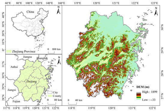
Figure 1.
Study area. Note: This map was created based on the standard map of China (Approval No. GS(2019)1822) downloaded from the Standard Map Service website of the National Geomatics Center of China, with no modifications made to the base map.
As one of China’s most economically developed provinces, Zhejiang recorded a GDP of CNY 9.01 trillion in 2024, ranking fourth among 31 provincial-level administrative regions in mainland China. The permanent resident population totals 66.7 million, with an urbanization rate of 75.5%. Topographically, the province exhibits a southwest-to-northeast descending gradient, characterized by diverse land forms including hills, basins, mountains, and plains, under a typical subtropical monsoon climate regime. During the study period, the average annual temperature ranged from 16.3 °C to 17.1 °C, with mean annual precipitation measuring 1443.8–1915.4 mm.
2.2. Data Sources and Processing
2.2.1. Sources and Processing of Land Use Data
This study utilizes four years of land use data (2005, 2010, 2015, 2020) with a 30 m spatial resolution, obtained from the Resource and Environmental Science Data Center of the Chinese Academy of Sciences. The datasets were generated through human–computer interactive interpretation and manual visual verification, achieving an overall accuracy exceeding 95% []. Land use types were classified into three primary categories encompassing eight secondary classes following established frameworks [] and regional characteristics, specifically the following: Production Space (PS) comprising APL and IML; Living Space (LS) including Urban Living Land (ULL) and Rural Living Land (RLL); and Ecological Space (ES) consisting of FEL, GEL, WEL, and Other Ecological Land (OEL). Subsequent reclassification of the land use data enabled systematic quantification of PLES spatial patterns and temporal dynamics.
2.2.2. Scale Selection and Processing
This study established four analytical scales: three administrative-unit scales (city, county, and township levels) and one grid scale. The grid size (5 km × 5 km) was determined based on the study area’s spatial extent, the resolution of land use data, and the related research []. Using the Fishnet tool in ArcGIS 10.8, a total of 4697 grids were generated. The average areas of provincial, city, county, and township units were 105, 104, 103, and 102 km2, respectively. City, county, and township scales were prioritized as China’s foundational administrative hierarchies, aligning with territorial spatial planning frameworks. The 5 km grid scale was selected to enable hierarchical transitions between administrative scales, ensuring effective integration of fundamental research and policy implementation.
2.2.3. Driving Factors’ Selection and Processing
Variations in EEQ are influenced by both stable factors (e.g., elevation, slope) and dynamic variables (e.g., precipitation, GDP, population). Seven driving factors were selected from natural and socio-economic categories, informed by previous studies [,] and regional characteristics. To mitigate multicollinearity among explanatory variables [], variance inflation factor (VIF) testing was conducted using SPSS 26. The results indicated that elevation and slope failed the VIF test. Following the exclusion of these two indicators, all remaining influencing factors demonstrated VIF values below 5, confirming the absence of multicollinearity issues. All selected indicators were converted to the “WGS_1984” coordinate system and resampled to corresponding analytical scales. Table 1 presents the finalized EEQ driving factor indicator system and the data sources corresponding to each selected factor.

Table 1.
Data sources of driving factors of EEQ.
2.2.4. Research Framework
The conceptual framework of this study is illustrated in Figure 2. Initially, the study area was delineated, followed by spatial data collection and preprocessing to establish scale selection and driving factor identification. Subsequently, land use transition characteristics were analyzed through land use transition matrices. Following this, the EEQ was quantified to assess its spatial distribution and temporal variations, with the ecological contribution rate of land use transition calculated. Finally, the explanatory power of dominant influencing factors and their interaction effects on EEQ were systematically examined.
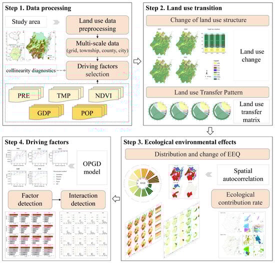
Figure 2.
Framework of research concepts.
2.3. Methods
2.3.1. Land Use Transfer Matrix
The land use transfer matrix is a tool used to quantify the mutual conversion between different land types over a specific period []. Based on data reclassification, this study employed a land use transfer matrix to analyze the area and proportional distribution of land use transition in the study area from 2005 to 2020. The mathematical expression is as follows:
where sij represents the area of land converted from type i to type j, and n denotes the total number of land use types.
2.3.2. Analysis of Ecological Environmental Effects from Land Use Transition
- EEQ index
The EEQ index is a widely adopted metric for quantifying ecological environmental effects. It evaluates regional ecological quality by integrating the ecological value and area proportion of different land use types []. Despite its limitation in overlooking site-specific heterogeneity, this approach does provide a direct representation of land use transition impacts on EEQ. The formula is
where EEQt represents the EEQ index of the study area at time t, Aki denotes the area of land use type i, TA is the total area, and Ri is the EEQ for land use type i. The Ri values in this study were derived from established values for all land use types (Table 2) []. The EEQ values corresponding to primary and secondary land use classifications can be derived using an area-weighted approach.
Table 2.
Ri values of land use types.
The EEQ index was classified into five categories based on the natural breaks method in ArcGIS 10.8: poor (0–0.25), fair (0.25–0.45), moderate (0.45–0.65), good (0.65–0.80), and excellent (0.80–1.00). Changes in EEQ were categorized as drastically degraded (≤−2%), mildly degraded (−1%), unchanged (0%), mildly improved (+1%), and drastically improved (≥+2%) [].
- Spatial autocorrelation analysis
Spatial autocorrelation analysis was employed to examine the spatial distribution patterns and interdependencies of EEQ, addressing spatial clustering and heterogeneity []. This method is currently widely used to analyze the relationship of EEQ between a given spatial unit and the surrounding area []. Global and local spatial autocorrelation analyses were conducted to assess the spatial dependence and clustering of EEQ. The formulas are
where Ii and I represent the local Moran’s I and global Moran’s I, respectively, n is the total number of spatial units, Xi and Xj represent EEQ values of units i and j, and Wij is the spatial weight matrix. This study defines the adjacency relationship in the spatial weight matrix using inverse distance weighting, where weights decrease as distance increases, with the distance method specified as Euclidean distance.
From the clustering maps generated by local spatial autocorrelation analysis, four types of spatial correlations can be identified: H-H indicates high EEQ indices in both the central unit and its surrounding areas, reflecting local positive spatial autocorrelation; H-L represents high EEQ units surrounded by low EEQ units, demonstrating local negative spatial autocorrelation; L-H describes low EEQ units encircled by high EEQ units, forming “depression zones” adjacent to high-value regions; and L-L signifies low EEQ indices in both the central unit and neighboring areas, characterizing localized degradation clusters.
- Ecological contribution rate of land use transition
The ecological contribution rate quantifies the impact of specific land use transition on EEQ, calculated based on changes in the EEQ index before and after transition []. The formula is
where LEI represents the ecological contribution rate of land use transition; LE denotes the EEQ index at either the initial or final stage of a specific land use change type; LA is the area of the land use change type; and TA is the total regional area.
2.3.3. OPGD Method
The Geodetector model is a spatial statistical method primarily used to detect spatial heterogeneity of variables []. While widely applied, its results are highly sensitive to data discretization methods. The OPGD method, developed as an extension of the Geodetector framework [], addresses limitations of the traditional Geodetector by identifying optimal combinations of discretization methods and scale parameters []. It is specifically designed to analyze influencing factors and their interactions in geographic spatial heterogeneity []. In this study, the “GD” package in RStudio 2025.05.1 was employed for factor detection and interaction detection. Five discretization methods were adopted, namely equal (equal interval), natural (natural breaks), quantile (quantile classification), geometric (geometric interval), and SD (standard deviation interval). The number of class intervals for each method was set to vary from 3 to 8, allowing for a comprehensive evaluation of discretization effects. Among all combinations of methods and interval numbers, the one producing the highest q-value was identified as the optimal discretization scheme for each driving factor. The factor detection formula is
where q represents the explanatory power of an independent variable on the dependent variable, ranging from [0, 1]. A higher q-value indicates stronger explanatory power, and vice versa.
Interaction detection evaluates whether the combined effect of two independent variables enhances, weakens, or independently influences the explanatory power on the dependent variable. The criteria for interaction types are defined as follows: nonlinear-enhance: q(X1∩X2) > q(X1) + q(X2); bi-variable enhance: Max [q(X1),q(X2)] < q(X1∩X2) < q(X1) + q(X2); nonlinear-weaken: q(X1∩X2) < Min [q(X1), q(X1)]; and uni-variable weaken: Min [q(X1), q(X2)] < q(X1∩X2) < Max [q(X1),q(X2)] [].
3. Results
3.1. Land Use Transition in Study Area
3.1.1. Change in Land Use Structure
PLESs in the study area ranked from highest to lowest as ES > PS > LS. The proportion of ES decreased from 69.10% in 2005 to 68.24% in 2020, representing a 1.24% reduction with a total area loss of 897.55 km2. Phase-specific analysis revealed accelerated decline in ES during 2005–2015, followed by a partial recovery in 2015–2020. The proportion of PS declined from 25.77% in 2005 to 25.69% in 2020, with a total area reduction of 88.00 km2, exhibiting a fluctuating “decline–rise–decline” pattern across periods. In contrast, the LS proportion gradually increased from 5.13% to 6.07%, with an area expansion of 985.55 km2 (18.40% growth), particularly marked during 2010–2015 (Table 3).
Table 3.
Area and change rate of PLES from 2005 to 2020.
In terms of secondary classification, the largest land use type was FEL, continuously covering over 60% of the total area and primarily distributed in mountainous area. This was followed by APL, occupying over 20% of the total area and mainly located in the plain area (Figure 3), highlighting forests and croplands as the two dominant land use types. In terms of change rates during the study period, the fastest-growing type was IML, with a 112.05% increase, followed by RLL (+19.88%) and ULL (+17.04%), aligning with the rapid industrialization and urbanization phases in the study area. Conversely, the most significant declines occurred in OEL (−19.08%), WEL (−10.92%), and APL (−6.19%).
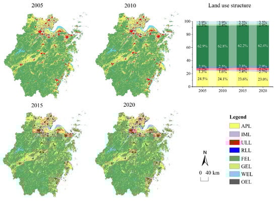
Figure 3.
Land use structure of different years in Zhejiang (2005–2020).
3.1.2. Land Use Transition Pattern
During the study period, the total area of land use transition reached 2925.95 km2 (2.80% of the study area), with APL outflows and IML inflows representing the dominant transfer types (Table 4). For PS, APL outflows totaled 1695.75 km2, primarily converted to IML (43.35%), RLL (27.47%), and ULL (25.62%). Temporal variations were observed: during 2005–2010, APL was mainly converted to IML (61.74%); in 2010–2015, transition shifted to IML (34.13%) and ULL (37.77%); and during 2015–2020, conversions redirected to FEL (40.35%), IML (26.86%), and RLL (26.10%). These patterns indicate that industrialization and urbanization partially encroached on croplands. IML inflows amounted to 1545.06 km2, predominantly sourced from APL (47.58%), FEL (26.95%), and WEL (21.24%).
Table 4.
Land use transfer matrix from 2005 to 2020 (unit: km2).
For LS, ULL and RLL inflows reached 476.21 km2 and 515.95 km2, respectively, with 91.21% of ULL and 90.27% of RLL originating from APL. Both categories exhibited peak expansion during 2010–2015. FEL outflows totaled 531.51 km2, largely converted to IML (78.35%), with transition concentrated in 2010–2015. This period also saw bidirectional conversions between FEL and APL, closely linked to the Grain-for-Green policy. Similarly, WEL outflows of 507.61 km2 were predominantly converted to IML (64.64%) (Figure 4).
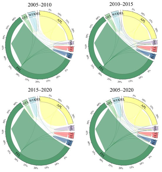
Figure 4.
Land use transfer at each stage.
3.2. Ecological Environmental Effects Based on Different Spatial Scales
3.2.1. Distribution of EEQ
At the provincial scale, the overall EEQ indexes of the study area in 2005, 2010, 2015, and 2020 were 0.675, 0.671, 0.665, and 0.666, respectively, indicating generally favorable EEQ with an accelerated degradation trend during 2005–2015 followed by partial recovery in 2015–2020. EEQ distributions varied across spatial scales: city and grid scales exhibited relative stability, while the county scale demonstrated the highest spatial heterogeneity.
At the city scale, the EEQ index ranged from 0.24 to 0.84, displaying a distinct southwest-to-northeast gradient. LS City, located in the mountainous southern region with high forest coverage and superior ecological conditions, consistently maintained the highest EEQ (excellent level) throughout the study period. In contrast, JX City, situated in the northern Hangjiahu Plain adjacent to Shanghai, showed the lowest EEQ due to extensive PS and LS expansion, insufficient ES, and pollution from textile industries. By 2020, JX’s EEQ had declined to a poor level (Figure 5). Notably, HZ and WZ achieved relatively high EEQ (second only to LS) by balancing economic development with ecological conservation, maintaining substantial proportions of ES.
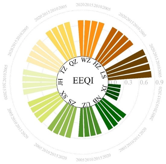
Figure 5.
EEQ index at city level. Notes: LS: Lishui, HZ: Hangzhou, WZ: Wenzhou, QZ: Quzhou, TZ: Taizhou, JH: Jinhua, SX: Shaoxing, ZS: Zhoushan, UZ: Huzhou, NB: Ningbo, JX: Jiaxing.
At the county scale, the EEQ distribution ranged from 0.16 to 0.87, exhibiting significant spatial heterogeneity characterized by “higher values in southern and western mountainous area and lower values in northeastern plains and coastal area”. During the study period, high-value EEQ index areas declined in coverage, while low-value areas remained stable. Specifically, the proportion of counties classified as excellent decreased from 30.3% in 2005 to 22.3% in 2020, whereas areas categorized as poor and fair showed minimal changes.
At the township scale, EEQ index spanned 0.09–0.93. Although areas classified as poor occupied a small proportion (1.1% in 2005 rising to 2.0% in 2020), their incremental growth signaled localized degradation. At the grid scale, EEQ index ranged from 0 to 0.95, with steep gradients between grids, though inter-annual variations in area proportions of each EEQ class remained relatively stable (Figure 6).
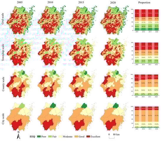
Figure 6.
Distribution of EEQ at different spatial scales.
In terms of spatial clustering patterns, global spatial autocorrelation analysis revealed that Moran’s I values across all four spatial scales were greater than 0, with p-values passing significance tests, indicating a clustered distribution of EEQ in study area. With the exception of the city scale, the p-values for spatial autocorrelation at the other three scales were consistently less than 0.001 across all study years, passing the 0.1% significance test. Overall, Moran’s I decreased sequentially from the county scale to the township, grid, and city scales, with the most pronounced spatial clustering observed at the county scale. However, Moran’s I for the EEQ index at the county scale declined by 0.03 during the study period, suggesting a slight increase in spatial dispersion and weakened spatial correlation, while changes in spatial autocorrelation at other scales remained negligible (Table 5).
Table 5.
Spatial autocorrelation of EEQ at different spatial scales.
Further local spatial autocorrelation analyses across scales revealed distinct clustering patterns. At the city scale, no significant EEQ clustering was observed during 2005–2010. By 2015 and 2020, however, JH and LS emerged as H-H clusters. At the county scale, pronounced clustering patterns were identified: the southwestern region, centered on LS, exhibited H-H clusters with spillover effects on neighboring areas, while the northeastern plains displayed L-L clustering, where low-EEQ zones were encircled by other low-EEQ units. At the township and grid scales, both H-H and L-L clusters increased significantly compared to the city and grid scales, reflecting finer-grained spatial heterogeneity (Figure 7).
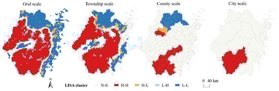
Figure 7.
Local spatial autocorrelation agglomeration distribution of EEQ (2020). Note: H: High, L: Low, N-S: Not Significant.
3.2.2. Change in EEQ
During the study period, city and county scales exhibited universal EEQ degradation, while township and grid scales showed spatiotemporal differentiation characterized by coexisting degradation and localized improvement. Across all scales, the 2010–2015 period marked accelerated EEQ degradation, with a notable slowdown in degradation trends after 2015. At the city scale, all 11 cities experienced EEQ declines, with degraded areas accounting for 65.7% of the total. Among these, JX and ZS recorded the largest declines at −3.30% and −2.13%, respectively. At the county scale, all 90 counties showed EEQ reductions, with drastically degraded counties concentrated in the northeastern plains and southeastern coastal counties. Degraded areas accounted for 30% of the total. At the township and grid scales, EEQ changes followed similar patterns: degraded units were widely distributed, covering 44.9% and 35.4% of the total area, respectively, while improved areas represented only 0.4% and 1.0% (Figure 8).
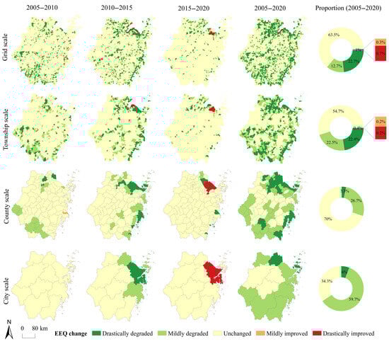
Figure 8.
Change in EEQ at different spatial scales.
3.2.3. Ecological Contribution Rate of Land Use Transition
The ecological contribution rates of land use transitions to EEQ in positive- and negative-effect areas were calculated separately (Figure 9a,b). In positive-effect areas, conversions of WEL and IML to GEL played pivotal roles, with contribution rates of 0.00015 and 0.00011, respectively. The primary driver of EEQ improvement was the large-scale conversion of intertidal flats in WEL to high-coverage grassland in GEL, accounting for 26.8% of the total contribution. Conversions of IML to GEL ranked second (19.3%), resulting from land remediation of abandoned industrial and mining sites converted to GEL.
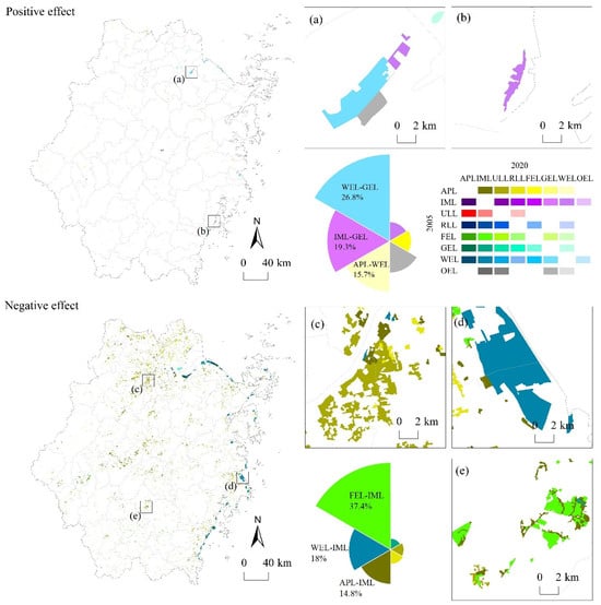
Figure 9.
Land use transition and ecological contribution rates from 2005 to 2020. (a,b) The typical area of the positive effect; (c–e) The typical area of the negative effect.
In negative-effect areas, EEQ degradation was predominantly driven by conversions of FEL, WEL, and APL to IML (Figure 9c–e), with contribution rates of 0.0026, 0.0012, and 0.0010 (37.4%, 18.0%, and 15.7% of the total contributions, respectively). These patterns indicate that EEQ degradation was primarily linked to IML expansion during industrialization. Urbanization-driven land development encroached on ES (e.g., FEL, WEL) and PS (primarily APL). In the northeastern plains, EEQ degradation mainly arose from APL and WEL conversions to IML, while in southwestern mountainous regions, FEL-to-IML transition dominated.
3.3. Driving Factors of EEQ at Different Scales
3.3.1. Single-Factor Analysis
Five continuous driving factors were discretized to identify optimal combinations of classification methods and spatial scale parameters for spatial data (Figure 10). Based on this, q-values under optimal spatial discretization were calculated (Figure 11). At the grid scale, all driving factors passed significance tests at the 0.1% level, with precipitation and NDVI ranking as the top two drivers. Precipitation exhibited the highest explanatory power (q > 0.8). At the township scale, all factors also passed 0.1% significance tests, with precipitation and GDP per unit area as the top two drivers, where precipitation’s explanatory power fluctuated around 0.6. At the county scale, all factors except precipitation in 2015 showed statistical significance. NDVI, GDP per unit area, and population density emerged as dominant drivers, with NDVI demonstrating the highest explanatory power (q > 0.8). At the city scale, precipitation failed significance tests in 2020, while the remaining factors were significant, all with q-values exceeding 0.8. Thus, dominant drivers of EEQ varied across spatial scales, yet natural factors consistently exhibited the strongest explanatory power at all scales. Socio-economic factors significantly influenced EEQ at county and city scales, with q-values exceeding 0.5.
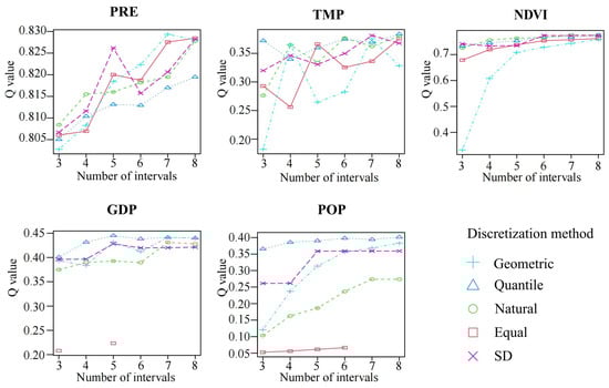
Figure 10.
Optimal spatial discretization for each driving factor (taking grid-scale data of 2020 as an example).
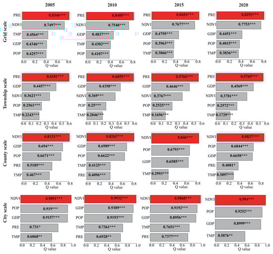
Figure 11.
Results of factor detection. Note: * p < 0.05, ** p < 0.01, *** p < 0.001; Red represents the factor with the highest q-value.
3.3.2. Factor Interaction Analysis
Factor interaction analysis revealed significant scale dependency (Figure 12). At the grid scale, interactions between precipitation and other factors diminished the individual explanatory power of single factors, while interactions among other factors enhanced their combined effects. The strongest interaction was observed between per-capita GDP and NDVI. At the township scale, interactions resulting in diminished explanatory power outnumbered enhanced ones, with the strongest interaction occurring between per-capita GDP and temperature. At the county scale, the interaction strength of all driving factors exceeded their individual explanatory power, with the strongest interactions observed between NDVI and precipitation, as well as per-capita GDP and NDVI. At the city scale, interactions among multiple factors approached 1, with the strongest interactions between precipitation and temperature, or precipitation and NDVI. Across all four scales, NDVI consistently emerged as one of the most influential factors in interactions, highlighting its critical role in shaping EEQ dynamics.
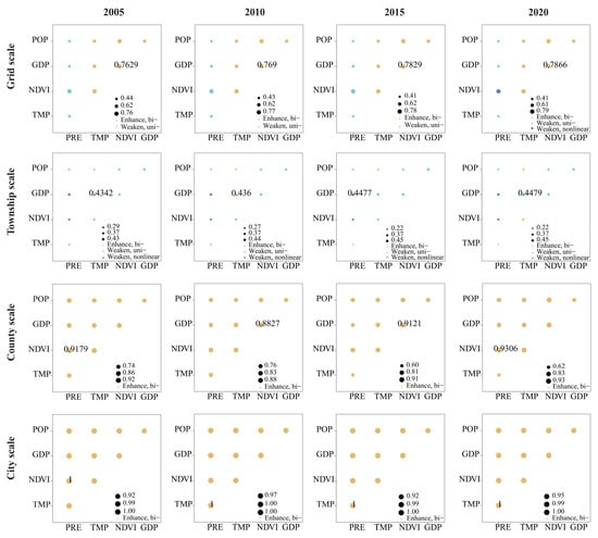
Figure 12.
Results of interaction detection. Note: The size of the circles represents the explanatory power of interactions between independent variables on the dependent variable.
4. Discussion
4.1. Scale Effects of EEQ
This study systematically reveals the scale-dependent characteristics and differentiation patterns of land use transition impacts on EEQ. Significant scale effects manifest in the spatial distribution, evolutionary trends, and driving mechanisms of EEQ. While most prior research has examined EEQ and its influencing factors at single spatial scales, neglecting the critical value of multi-scale analyses [], this investigation conducts multi-scale assessments to evaluate EEQ spatial characteristics and primary drivers across grid, township, county, and municipal scales. The principal contributions are as follows:
- Clarifying scale-dependent differentiation in spatial heterogeneity. The findings demonstrate scale dependency in land use transition impacts on EEQ, consistent with earlier research []. The county scale exhibits the strongest spatial heterogeneity (Moran’s I > 0.87, p < 0.001), establishing it as the core unit for EEQ spatial differentiation—a conclusion corroborated by recent studies []. This phenomenon stems from the intensive coupling of natural endowments (e.g., topographic gradients between southwestern mountains and northeastern plains) and socio-economic activities within counties. Mountainous counties maintain superior EEQ due to high forest coverage, whereas plain counties face stronger degradation pressures from IML expansion []. In contrast, city scales show pronounced spatial homogenization effects due to larger administrative units, obscuring internal variations []. Although 5 km grid scales detect localized anomalies (e.g., abrupt EEQ declines in urban–rural fringes), misalignment between regular grids and administrative boundaries limits their direct utility for management decisions. The township scale demonstrates transitional characteristics, with heterogeneity levels intermediate between county and grid scales.
- Discussing scale dependency in EEQ evolutionary trends. Land use transition exhibits distinct scale-dependent ecological effects. Macro-scale analyses (city and county levels) reveal universal EEQ degradation, particularly during the 2010–2015 industrialization acceleration phase, where IML encroachment on ES drove rapid deterioration. Conversely, micro-scale assessments (township and grid levels) uncover localized improvements obscured at coarser resolutions: post-2015, approximately 0.4% of townships and 1.0% of grids showed EEQ enhancement, primarily attributable to restorative transitions such as abandoned industrial sites (WEL/IML) converted to GEL. This “macro-scale degradation coexisting with micro-scale improvement” dichotomy underscores the critical function of grid- and township-level analyses in identifying site-specific ecological recovery. Empirical evidence confirms that EEQ variations diminish at broader scales while intensifying at finer resolutions [], as finer-scale land transitions simultaneously drive and respond to macro-scale dynamics, collectively shaping EEQ outcomes []. Specifically, larger spatial units face greater implementation barriers and extended timeframes for land use transitions []. Localized EEQ demonstrates heightened sensitivity to land use changes—urban expansion and agricultural land reduction directly compromise ecological functions during urbanization. Smaller-scale transitions may further trigger environmental issues (e.g., soil erosion, degradation), exacerbating EEQ decline. Conversely, proactive land use optimization at finer scales directly contributes to significant EEQ recovery [].
- Illustrating the scale transition of EEQ driving factors. Natural factors constitute primary cross-scale determinants of EEQ, aligning with extensive research []. Precipitation predominantly influences EEQ at micro scales, where its variability regulates biochemical processes and nutrient cycling in surface ecosystems, exerting critical explanatory power over localized EEQ patterns []. Socio-economic factors gain prominence with increasing spatial extent, demonstrating significant negative effects at city and county scales: a higher per-capita GDP and population density correlate with lower EEQ (Figure 13). That is, the development of urbanization is accompanied by a decrease in EEQ, and this result is also consistent with the relevant studies [].
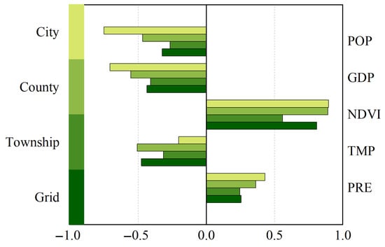
Figure 13.
Comparison of Pearson correlation analysis for all factors at different scales.
The observed multi-scale effects substantiate that single-scale analyses may introduce biases into ecological management strategies. The county scale emerges as the optimal unit for balancing ecological conservation with developmental demands, owing to its concurrent high spatial heterogeneity and policy implementability. Meanwhile, the grid scale’s capacity to identify localized restoration provides scientific foundations for targeted implementation of ecological engineering. These findings not only deepen the understanding of multi-scale EEQ research but also methodologically validate the necessity of integrated multi-scale analysis for investigating complex human–environment systems.
4.2. Policy Impacts on Land Use Transition and EEQ
While policy variables significantly influence land use transition and EEQ [,], data limitations precluded their quantitative integration into our analytical framework. The inherent complexity of policy factors—including implementation intensity, regional heterogeneity, and dynamic adjustments—presents challenges for systematic quantification. Nevertheless, through a contextual analysis of key land management policies and ecological initiatives during the study period, we preliminarily elucidated policy-mediated regulatory mechanisms:
Phase I (2005–2010): Rural Land Consolidation. The “Thousand-Village Demonstration, Ten-Thousand-Village Renovation Project” prioritized rural land remediation. Policy interventions focused on APL optimization through homestead reclamation, infrastructural upgrades, and orderly conversion to LS. This phase enhanced rural habitat quality and land use efficiency while reducing cropland abandonment []. IML expansion remained limited. By consolidating settlement patterns and mitigating land fragmentation, policies indirectly preserved ES integrity. Although EEQ experienced a gradual decline, these foundational interventions established baseline conditions for subsequent ecological stabilization.
Phase II (2010–2015): Industrial Expansion and Ecological Restoration. Accelerated industrialization shifted the policy emphasis toward economic development, triggering “PS encroachment on ES” transitions. Rapid conversion of APL to IML, coupled with mining and transportation infrastructural expansion, intensified ecological fragmentation. EEQ consequently declined to its lowest values. However, parallel ecological restoration policies (e.g., steep-slope cropland retirement) provided localized mitigation. This dualistic policy outcome manifested as (1) economic growth agendas exacerbating land use conflicts; and (2) targeted ecological projects containing degradation in critical functional zones, establishing foundations for future recovery.
Phase III (2015–2020): Ecological Prioritization and Transition Restructuring. Zhejiang’s strategic pivot toward “ecological primacy and green development” expanded policy scopes from land remediation to holistic ecosystem enhancement. Flagship initiatives included the “Ecosystem Product Value Realization Mechanism” and “Abandoned Industrial Land Greening Program,” which maximized ecological benefits through targeted transitions (e.g., WEL/IML→GEL). The empirical results confirm GEL expansion and IML growth deceleration during this phase. Policy-driven transitions exhibited dual regulation: (1) ES connectivity improved through GEL restoration; and (2) stringent industrial land approvals suppressed uncontrolled expansion, converting inefficient IML to ES. Consequently, EEQ stabilized, with localized improvements observable at the township scale. Enhanced synergy between policies and natural factors signified the preliminary transition from economic-centric to eco-economic balanced land governance [].
4.3. Policy Recommendations for Optimizing EEQ
This study offers novel insights with policy implications for land use and EEQ management in the study area and beyond, providing scientific recommendations to promote sustainable land use transition. The policy implications are summarized as follows:
- Establishment of multi-scale differentiated EEQ management frameworks. First, this requires the clarification of EEQ management priorities across scales. Given the scale dependency of EEQ revealed in this study, policymakers should adopt multi-scale perspectives to address various EEQ characteristics and governance needs. Policy implementation scales should be adjusted based on the relative contributions of driving factors at different scales to maximize the efficiency of EEQ management. Macro-scale policies should emphasize EEQ integrity by integrating natural and socio-economic factors, while micro-scale policies should target localized ecological challenges through precision management, particularly in terms of addressing climatic drivers such as precipitation. Second, county-scale EEQ governance should be prioritized. This study identified the county scale as the optimal unit for EEQ management, aligning with China’s recent urbanization strategy centered on county-level development. In practice, county-scale governance should leverage the unique role of counties in bridging urban and rural systems.
- Maintenance and improvement of EEQ through the rational restructuring of land use. First, the coordinated development of PLESs should be promoted. The present findings demonstrate that the direction and magnitude of the PLES transition had a direct effect on EEQ. Urbanization policies should therefore incentivize a balanced integration of production, living, and ecological functions to ensure sustainable land use. Comprehensive land remediation should be prioritized to optimize existing land resources and enhance utilization efficiency. Concurrently, ES regulations should be strengthened by the rigorous delineation and management of ecological redlines, ensuring the protection of ecologically sensitive zones and critical functional areas. Second, multi-scale land use planning and integrated assessments should be prioritized, together with the establishment of hierarchical land use planning systems tailored to scale-specific characteristics, the development of science-based policies to encourage sustainable land use practices [], and the implementation of adaptable monitoring frameworks to evaluate ecological impacts of land use changes, ensuring planning flexibility and responsiveness.
- Implementation of zonal EEQ management strategies. First, EEQ conservation in mountainous areas should be prioritized. Ecological monitoring and assessment systems should be implemented in mountainous regions and zones, and robust ecological compensation mechanisms should be established to mitigate the effects of development. Second, EEQ degradation should be curtailed in coastal regions and plains. Strategies for green development should be implemented to decouple rapid economic growth from ecological degradation. Low-impact land use transitions should be prioritized, including the integration of renewable energy infrastructure and restoration of coastal wetlands, to minimize adverse effects on EEQ.
4.4. Limitations and Future Research Directions
This study has several limitations that require further refinement. First, EEQ was calculated solely in terms of land use types, neglecting other contributing factors. Second, the selection of spatial scales focused on four categories, without accounting for the scale dependency associated with varying grid dimensions. This limitation precluded the examination of ecological processes within finer-scale natural units with ecological significance [] and did not explore heterogeneity across grids of varying sizes. Third, intra-regional EEQ variability, such as differences between metropolitan, mountainous, and coastal zones, was not systematically compared. Lastly, while natural and socio-economic factors were prioritized as drivers, other potential influences (e.g., policy implementation, industrial development, location conditions, infrastructure, and public services) were not addressed.
Future research should integrate emerging technologies (e.g., remote sensing, big data analytics) to assess ecological impacts across multiple dimensions. Additionally, exploratory investigations should address the scale dependency of EEQ corresponding to varying grid sizes and geometries, while conducting in-depth analyses of EEQ at significantly finer resolutions. Cross-regional comparative studies are needed to elucidate commonalities and divergences in land use transition effects in different geographical and socio-economic contexts. Additionally, advanced modeling frameworks should investigate nonlinear relationships between EEQ and its drivers, such as threshold effects and synergistic interactions.
5. Conclusions
This study analyzed land use pattern changes in the study area and explored the impacts of land use transition on EEQ across four spatial scales (city, county, township, and grid), identifying key driving factors. The main findings are summarized as follows:
The PLES area distribution ranked from largest to smallest as ES > PS > LS, with FEL being the dominant secondary category, consistently covering over 60% of the total area. Land use transition occurred across 2.80% of the study area during the study period, primarily characterized by APL outflows and IML inflows. The most intensive transition period was 2010–2015.
The EEQ index fluctuated between 0.665 and 0.675, exhibiting significant scale dependency. Moran’s I values decreased sequentially from the county scale to township, grid, and city scales, with the strongest spatial clustering observed at the county scale, indicating maximum spatial heterogeneity of EEQ at this level.
City and county scales exhibited universal EEQ degradation, whereas township and grid scales showed coexisting degradation and localized improvement. In positive-effect zones, conversions of WEL and IML to GEL played pivotal roles. In negative-effect zones, EEQ degradation was primarily driven by conversions of FEL, WEL, and APL to IML.
EEQ drivers also demonstrated scale dependency. Analysis revealed that precipitation was the primary driving factor for EEQ at the grid and township scales, while NDVI dominated at the county and city scales, confirming natural factors as primary cross-scale influencers. Socio-economic factors exerted significant effects only at the city and county scales.
Author Contributions
Conceptualization, Z.X.; methodology, Z.X.; software, Z.X.; validation, Z.X.; formal analysis, Z.X.; investigation, Z.X.; resources, Z.X.; data curation, Z.X.; writing—original draft preparation, Z.X.; writing—review and editing, Z.X.; visualization, Z.X. and H.Z.; supervision, Z.X. and F.K.; project administration, Z.X. and J.Y.; funding acquisition, Z.X. and F.K. All authors have read and agreed to the published version of the manuscript.
Funding
This research was funded by the Zhejiang Academy of Agricultural Sciences, grant number 2025R18Y11E11.
Data Availability Statement
The raw data supporting the conclusions of this article will be made available by the authors on request.
Conflicts of Interest
The authors declare no conflicts of interest. The funders had no role in the design of this study; in the collection, analyses, or interpretation of data; in the writing of the manuscript; or in the decision to publish the results.
Abbreviations
The following abbreviations are used in this manuscript:
| EEQ | Ecological environment quality |
| OPGD | Optimal parameter geographic detector |
| PLESs | Production, living, and ecological spaces |
| PS | Production space |
| LS | Living space |
| ES | Ecological space |
| APL | Agricultural production land |
| IML | Industrial and mining land |
| ULL | Urban living land |
| RLL | Rural living land |
| FEL | Forest ecological land |
| GEL | Grassland ecological land |
| WEL | Water ecological land |
| OEL | Other ecological land |
References
- Turner Ii, B.L.; Skole, D.; Sanderson, S.; Fischer, G.; Fresco, L.; Leemans, R. Land-Use and Land-Cover Change: Science/Research Plan; IGBP: Stockholm, Sweden, 1995. [Google Scholar]
- GLP. Science Plan and Implementation Strategy Global Land Project; IGBP Report No.53; IGBP: Stockholm, Sweden, 2005. [Google Scholar]
- Song, X.P.; Hansen, M.C.; Stehman, S.V.; Potapov, P.V.; Tyukavina, A.; Vermote, E.F.; Townshend, J.R. Global land change from 1982 to 2016. Nature 2018, 560, 639. [Google Scholar] [CrossRef]
- Fu, B.; Zhang, J.; Wu, X.; Meadows, M.E. Geography’s hotspots and frontiers: Diverse, systematic, and intelligent trends. Geogr. Sustain. 2025, 6, 100285. [Google Scholar] [CrossRef]
- Levin, S.; Xepapadeas, T.; Crépin, A.; Norberg, J.; de Zeeuw, A.; Folke, C.; Hughes, T.; Arrow, K.; Barrett, S.; Daily, G.; et al. Social-ecological systems as complex adaptive systems: Modeling and policy implications. Environ. Dev. Econ. 2013, 18, 111–132. [Google Scholar] [CrossRef]
- Ostrom, E. A diagnostic approach for going beyond panaceas. Proc. Natl. Acad. Sci. USA 2007, 104, 15181–15187. [Google Scholar] [CrossRef]
- Zhao, Q.; Yu, L.; Chen, X. Land system science and its contributions to sustainable development goals: A systematic review. Land Use Policy 2024, 143, 107221. [Google Scholar] [CrossRef]
- Yu, B.B. Ecological effects of new-type urbanization in china. Renew. Sust. Energ. Rev. 2021, 135, 110239. [Google Scholar] [CrossRef]
- Zhu, T.; Qin, X. Urbanization path: The fundamental problem of changes in land use patterns. Sci. Geogr. Sin. 2012, 32, 1348–1352. [Google Scholar]
- Tao, J.; Lu, Y.; Ge, D.; Dong, P.; Gong, X.; Ma, X. The spatial pattern of agricultural ecosystem services from the production-living-ecology perspective: A case study of the huaihai economic zone, china. Land Use Policy 2022, 122, 106355. [Google Scholar] [CrossRef]
- Li, W.J.; Wang, Y.; Xie, S.Y.; Cheng, X. Coupling coordination analysis and spatiotemporal heterogeneity between urbanization and ecosystem health in chongqing municipality, china. Sci. Total Environ. 2021, 791, 148311. [Google Scholar] [CrossRef]
- Li, H. Introduction to the Research of Marginalization of Agricultural Land; China Social Sciences Press: Beijing, China, 2023. [Google Scholar]
- Meyfroidt, P.; Roy Chowdhury, R.; de Bremond, A.; Ellis, E.C.; Erb, K.H.; Filatova, T.; Garrett, R.D.; Grove, J.M.; Heinimann, A.; Kuemmerle, T.; et al. Middle-range theories of land system change. Glob. Environ. Change 2018, 53, 52–67. [Google Scholar] [CrossRef]
- Dadashpoor, H.; Azizi, P.; Moghadasi, M. Land use change, urbanization, and change in landscape pattern in a metropolitan area. Sci. Total Environ. 2019, 655, 707–719. [Google Scholar] [CrossRef]
- Hou, Y.; Chen, Y.; Ding, J.; Li, Z.; Li, Y.; Sun, F. Ecological impacts of land use change in the arid tarim river basin of china. Remote Sens. 2022, 14, 1894. [Google Scholar] [CrossRef]
- Yang, L.; Liu, Y.; Liu, Y.; Liu, R. Spatial-temporal dynamics and drivers of ecosystem service interactions along the yellow river area in shaanxi province. J. Clean. Prod. 2025, 496, 145095. [Google Scholar] [CrossRef]
- Gari, S.R.; Newton, A.; Icely, J.D. A review of the application and evolution of the DPSIR framework with an emphasis on coastal social-ecological systems. Ocean Coast. Manag. 2015, 103, 63–77. [Google Scholar] [CrossRef]
- Liao, C. Quantitative judgement and classification system for coordinated development of environment and economy—A case study of the city group in the pearl river delta. Trop. Geogr. 1999, 19, 171–177. [Google Scholar]
- Giampietro, M.; Mayumi, K.; Ramos-Martin, J. Multi-scale integrated analysis of societal and ecosystem metabolism (MuSIASEM): Theoretical concepts and basic rationale. Energy 2009, 34, 313–322. [Google Scholar] [CrossRef]
- Li, J.S.; Sun, W.; Li, M.Y.; Meng, L.L. Coupling coordination degree of production, living and ecological spaces and its influencing factors in the yellow river basin. J. Clean. Prod. 2021, 298, 126803. [Google Scholar] [CrossRef]
- Song, W.; Deng, X.Z. Land-use/land-cover change and ecosystem service provision in china. Sci. Total Environ. 2017, 576, 705–719. [Google Scholar] [CrossRef] [PubMed]
- Newbold, T.; Hudson, L.N.; Hill, S.; Contu, S.; Lysenko, I.; Senior, R.A.; Börger, L.; Bennett, D.J.; Choimes, A.; Collen, B.; et al. Global effects of land use on local terrestrial biodiversity. Nature 2015, 520, 45. [Google Scholar] [CrossRef]
- Li, J.F.; Han, J.C.; Zhang, Y.; Liu, S.Q.; Ye, H.P.; Zhang, Z.Y. Decoupling characteristics of county-level land use carbon emissions and ecological environment quality at spatiotemporal scales: A case study of shaanxi province, china. Int. J. Digit. Earth 2024, 17, 2436494. [Google Scholar] [CrossRef]
- Peng, J.; Tian, L.; Liu, Y.X.; Zhao, M.Y.; Hu, Y.N.; Wu, J.S. Ecosystem services response to urbanization in metropolitan areas: Thresholds identification. Sci. Total Environ. 2017, 607, 706–714. [Google Scholar] [CrossRef] [PubMed]
- Qiao, H.; Kang, Y.; Niu, Y. Spatiotemporal dynamics and driving factors of ecosystem services value in lanzhou city, china. Sci. Rep. 2024, 14, 26562. [Google Scholar] [CrossRef]
- Su, Y.; Feng, G.; Ren, J. Spatio-temporal evolution of land use and its eco-environmental effects in the caohai national nature reserve of china. Sci. Rep. 2023, 13, 20150. [Google Scholar] [CrossRef]
- Gu, G.H.; Wu, B.; Lu, S.Q.; Zhang, W.Z.; Tian, Y.C.; Lu, R.C.; Feng, X.L.; Liao, W.H. Differential evolution of territorial space and effects on ecological environment quality in china’s border regions. J. Geogr. Sci. 2024, 34, 1109–1127. [Google Scholar] [CrossRef]
- Cao, Y.; Zhang, M.Y.; Zhang, Z.Y.; Liu, L.; Gao, Y.; Zhang, X.Y.; Chen, H.J.; Kang, Z.W.; Liu, X.Y.; Zhang, Y. The impact of land-use change on the ecological environment quality from the perspective of production-living-ecological space: A case study of the northern slope of tianshan mountains. Ecol. Inform. 2024, 83, 102795. [Google Scholar] [CrossRef]
- Walther, G.; Post, E.; Convey, P.; Menzel, A.; Parmesan, C.; Beebee, T.J.C.; Fromentin, J.; Hoegh-Guldberg, O.; Bairlein, F. Ecological responses to recent climate change. Nature 2002, 416, 389–395. [Google Scholar] [CrossRef]
- Wang, X.; Liu, G.; Xiang, A.; Xiao, S.; Lin, D.; Lin, Y.; Lu, Y. Terrain gradient response of landscape ecological environment to land use and land cover change in the hilly watershed in south china. Ecol. Indic. 2023, 146, 109797. [Google Scholar] [CrossRef]
- Li, C.; Wu, J. Land use transformation and eco-environmental effects based on production-living-ecological spatial synergy: Evidence from shaanxi province, china. Environ. Sci. Pollut. Res. 2022, 29, 41492–41504. [Google Scholar] [CrossRef]
- Hu, X.S.; Xu, H.Q. A new remote sensing index for assessing the spatial heterogeneity in urban ecological quality: A case from fuzhou city, china. Ecol. Indic. 2018, 89, 11–21. [Google Scholar] [CrossRef]
- Sun, Z.H.; Han, J.C.; Li, Y.A.; Yang, L.Y.; Lei, S.; Yan, J.K. Effects of large-scale land consolidation projects on ecological environment quality: A case study of a land creation project in yan’an, china. Environ. Int. 2024, 183, 108392. [Google Scholar]
- Lambin, E.F.; Meyfroidt, P. Global land use change, economic globalization, and the looming land scarcity. Proc. Natl. Acad. Sci. USA 2011, 108, 3465–3472. [Google Scholar] [CrossRef]
- Pattee, H.H. Hierarchy theory: The challenge of complex systems. In National Association of Biology Teachers; George Braziller Inc.: New York, NY, USA, 1973; Volume 35, pp. 428–429. [Google Scholar]
- Chen, W.Y.; Zhao, R.F.; Lu, H.T. Response of ecological environment quality to land use transition based on dryland oasis ecological index (DOEI) in dryland: A case study of oasis concentration area in middle heihe river, china. Ecol. Indic. 2024, 165, 112214. [Google Scholar] [CrossRef]
- Sun, T.; Yang, Y.; Wang, Z.; Yong, Z.; Xiong, J.; Ma, G.; Li, J.; Liu, A. Spatiotemporal variation of ecological environment quality and extreme climate drivers on the qinghai-tibetan plateau. J. Mt. Sci. 2023, 20, 2282–2297. [Google Scholar] [CrossRef]
- Ye, B.; Sun, B.; Shi, X.; Zhao, Y.; Pang, J.; Guo, Y.; Yao, W. Land use changes and its impact on ecological environment quality in bayannur city. Huan Jing Ke Xue Huanjing Kexue 2024, 45, 6899–6909. [Google Scholar]
- Zhou, G.; Long, H. Explanation of land-use system evolution: Modes, trends, and mechanisms. Land Use Policy 2025, 150, 107470. [Google Scholar] [CrossRef]
- Dang, L.; Zhao, F.; Teng, Y.; Teng, J.; Zhan, J.; Zhang, F.; Liu, W.; Wang, L. Scale dependency of trade-offs/synergies analysis of ecosystem services based on bayesian belief networks: A case of the yellow river basin. J. Environ. Manag. 2025, 375, 124410. [Google Scholar] [CrossRef] [PubMed]
- Li, K.; Wu, W.; Tian, S.; Li, L.; Li, Z.; Cao, Y. Geographical feature and method factors significantly influence the reliability of ecological source information transmission at multi-scale. Ecol. Indic. 2025, 170, 113029. [Google Scholar] [CrossRef]
- Bao, S.W.; Cui, W.L.; Yang, F. Future land use prediction and optimization strategy of zhejiang greater bay area coupled with ecological security multi-scenario pattern. PLoS ONE 2024, 19, e0291570. [Google Scholar] [CrossRef] [PubMed]
- Xu, Z.; Ke, F.; Yu, J. Spatio-temporal evolution and influencing factors of rural production-living-ecological function: A case study of mountainous counties in zhejiang province, china. Front. Environ. Sci. 2025, 13, 1495778. [Google Scholar] [CrossRef]
- Ning, J.; Liu, J.Y.; Kuang, W.H.; Xu, X.L.; Zhang, S.W.; Yan, C.Z.; Li, R.D.; Wu, S.X.; Hu, Y.F.; Du, G.M.; et al. Spatiotemporal patterns and characteristics of land-use change in china during 2010–2015. J. Geogr. Sci. 2018, 28, 547–562. [Google Scholar] [CrossRef]
- Yang, Q.; Duan, X.; Wang, L.; Jin, Z. Land use transformation based on ecological-production-living spaces and associated eco-environment effects: A case study in the yangtze river delta. Sci. Geogr. Sin. 2018, 38, 97–106. [Google Scholar]
- Huang, Y.; Lin, J.; He, X.; Lin, Z.; Wu, Z.; Zhang, X. Assessing the scale effect of urban vertical patterns on urban waterlogging: An empirical study in shenzhen. Environ. Impact Assess. Rev. 2024, 106, 107486. [Google Scholar] [CrossRef]
- Huang, J.T.; Zhang, Y.C.; Zhang, J.Q.; Qi, J.W.; Liu, P. Study on the ecological environment quality and its driving factors of the spatial transformation of production-living-ecological space in baishan city. Sci. Rep. 2024, 14, 18709. [Google Scholar] [CrossRef]
- Hayes, A.F.; Cai, L. Using heteroskedasticity-consistent standard error estimators in OLS regression: An introduction and software implementation. Behav. Res. Methods 2007, 39, 709–722. [Google Scholar] [CrossRef]
- Hu, J.; Miao, C. CHM\_PRE v2: A New Upgraded High-Precision Gridded Precipitation Dataset Considering Spatiotemporal and Physical Correlations for Mainland China; Zenodo: Geneva, Switzerland, 2025. [Google Scholar]
- Peng, S. 1-km Monthly Mean Temperature Dataset for China (1901–2023); National Tibetan Plateau Data Center: Beijing, China, 2024. [Google Scholar]
- Didan, K. MOD13a3 MODIS/terra Vegetation Indices Monthly l3 Global 1km SIN Grid v006; NASA EOSDIS Land Processes Distributed Active Archive Center: Sioux Falls, SD, USA, 2015.
- Xu, X. 1 km-Grid Dataset of Spatial Distribution of China’s GDP. Available online: https://www.resdc.cn/DOI/DOI.aspx?DOIID=33 (accessed on 21 April 2025).
- Hu, C.; Song, M.; Zhang, A. Dynamics of the eco-environmental quality in response to land use changes in rapidly urbanizing areas: A case study of wuhan, china from 2000 to 2018. J. Geogr. Sci. 2023, 33, 245–265. [Google Scholar] [CrossRef]
- Li, X.; Fang, C.; Huang, J.; Mao, H. The urban land use transformations and associated effects on eco-environment in nothwest china arid region: A case study in hexi region, gansu province. Quat. Sci. 2003, 23, 280–290. [Google Scholar]
- Zhang, Y.; Liu, Y.; Gu, J. Land use/land cover change and its environmental effects in wuhan city. Geogr. Sci. 2011, 31, 1280–1285. [Google Scholar]
- Yang, L.; Shi, L.; Wei, J.; Wang, Y. Spatiotemporal evolution of ecological environment quality in arid areas based on the remote sensing ecological distance index: A case study of yuyang district in yulin city, china. Open Geosci. 2021, 13, 1701–1710. [Google Scholar] [CrossRef]
- Anselin, L. Local indicators of spatial association-LISA. Geogr. Anal. 1995, 27, 93–115. [Google Scholar] [CrossRef]
- Zhou, Y.; Cao, W.; Zhou, J. Land-use transfer and its ecological effects in rapidly urbanizing areas: A case study of nanjing, china. Sustainability 2024, 16, 10615. [Google Scholar] [CrossRef]
- Lv, L.; Zhou, S.; Zhou, B.; Dai, L.; Chang, T.; Bao, G.; Zhou, H.; Li, Z. Land use transformation and its eco-environmental response in process of the regional development: A case study of jiangsu province. Sci. Geogr. Sin. 2013, 33, 1442–1449. [Google Scholar]
- Wang, J.; Zhang, T.; Fu, B. A measure of spatial stratified heterogeneity. Ecol. Indic. 2016, 67, 250–256. [Google Scholar] [CrossRef]
- Song, Y.; Wang, J.; Ge, Y.; Xu, C. An optimal parameters-based geographical detector model enhances geographic characteristics of explanatory variables for spatial heterogeneity analysis: Cases with different types of spatial data. GISci. Remote Sens. 2020, 57, 593–610. [Google Scholar] [CrossRef]
- Wang, D.; Zhang, L.; Yu, H.; Zhong, Q.; Zhang, G.; Chen, X.; Zhang, Q. Attributing spatially stratified heterogeneity in biodiversity of urban–rural interlaced zones based on the OPGD model. Ecol. Inform. 2024, 83, 102789. [Google Scholar] [CrossRef]
- Hou, M.; Deng, Y.; Yao, S. Coordinated relationship between urbanization and grain production in china: Degree measurement, spatial differentiation and its factors detection. J. Clean. Prod. 2022, 331, 129957. [Google Scholar] [CrossRef]
- Wang, J.; Xu, C. Geodetector: Principle and prospective. Acta Geogr. Sin. 2017, 72, 116–134. [Google Scholar]
- Zhang, X.M.; Fan, H.B.; Hou, H.; Xu, C.Q.; Sun, L.; Li, Q.Y.; Ren, J.Z. Spatiotemporal evolution and multi-scale coupling effects of land-use carbon emissions and ecological environmental quality. Sci. Total Environ. 2024, 922, 171149. [Google Scholar] [CrossRef]
- Xue, C.; Chen, X.; Xue, L.; Zhang, H.; Chen, J.; Li, D. Modeling the spatially heterogeneous relationships between tradeoffs and synergies among ecosystem services and potential drivers considering geographic scale in bairin left banner, china. Sci. Total Environ. 2023, 855, 158834. [Google Scholar] [CrossRef] [PubMed]
- Liu, Q.; Qiao, J.; Li, M.; Huang, M. Spatiotemporal heterogeneity of ecosystem service interactions and their drivers at different spatial scales in the yellow river basin. Sci. Total Environ. 2024, 908, 168486. [Google Scholar] [CrossRef]
- Chen, Y.; Lu, Y.; Meng, R.; Li, S.; Zheng, L.; Song, M. Multi-scale matching and simulating flows of ecosystem service supply and demand in the wuhan metropolitan area, china. J. Clean. Prod. 2024, 476, 143648. [Google Scholar] [CrossRef]
- Magliocca, N.R.; Dhungana, P.; Sink, C.D. Review of counterfactual land change modeling for causal inference in land system science. J. Land Use Sci. 2023, 18, 1–24. [Google Scholar] [CrossRef]
- Long, H. Theorizing land use transitions: A human geography perspective. Habitat Int. 2022, 128, 102669. [Google Scholar] [CrossRef]
- Tian, F.; Li, X.; Wu, X.; Gong, L. Identifying supply–demand mismatches of ecosystem services and social-ecological drivers at different scales to support land use planning. Ecol. Indic. 2025, 174, 113462. [Google Scholar] [CrossRef]
- Qiu, H.; Bai, Y.; Han, H.; Zhang, J.; Cheng, X. Ecosystem service supply and demand relationship and spatial identification of driving threshold in loess plateau of china. Ecol. Eng. 2025, 212, 107534. [Google Scholar] [CrossRef]
- Zhou, D.; Xu, J.C.; Lin, Z.L. Conflict or coordination? Assessing land use multi-functionalization using production-living-ecology analysis. Sci. Total Environ. 2017, 577, 136–147. [Google Scholar] [CrossRef]
- Foley, J.A.; DeFries, R.; Asner, G.P.; Barford, C.; Bonan, G.; Carpenter, S.R.; Chapin, F.S.; Coe, M.T.; Daily, G.C.; Gibbs, H.K.; et al. Global consequences of land use. Science 2005, 309, 570–574. [Google Scholar] [CrossRef]
- Turner, B.L.; Lambin, E.F.; Reenberg, A. The emergence of land change science for global environmental change and sustainability. Proc. Natl. Acad. Sci. USA 2007, 104, 20666–20671. [Google Scholar] [CrossRef]
- Su, X.Y.; Fan, Y.M.; Wen, C.H. Systematic coupling and multistage interactive response of the urban land use efficiency and ecological environment quality. J. Environ. Manag. 2024, 365, 121584. [Google Scholar] [CrossRef] [PubMed]
- Huber, P.R.; Greco, S.E.; Thorne, J.H. Spatial scale effects on conservation network design: Trade-offs and omissions in regional versus local scale planning. Landsc. Ecol. 2010, 25, 683–695. [Google Scholar] [CrossRef]
- Valerio, F.; Godinho, S.; Ferraz, G.; Pita, R.; Gameiro, J.; Silva, B.; Marques, A.T.; Silva, J.P. Multi-temporal remote sensing of inland surface waters: A fusion of sentinel-1&2 data applied to small seasonal ponds in semiarid environments. Int. J. Appl. Earth Obs. Geoinf. 2024, 135, 104283. [Google Scholar]
Disclaimer/Publisher’s Note: The statements, opinions and data contained in all publications are solely those of the individual author(s) and contributor(s) and not of MDPI and/or the editor(s). MDPI and/or the editor(s) disclaim responsibility for any injury to people or property resulting from any ideas, methods, instructions or products referred to in the content. |
© 2025 by the authors. Licensee MDPI, Basel, Switzerland. This article is an open access article distributed under the terms and conditions of the Creative Commons Attribution (CC BY) license (https://creativecommons.org/licenses/by/4.0/).