Structural Evolution of the Coastal Landscape in Klaipėda Region, Lithuania: 125 Years of Political and Sociocultural Transformations

Abstract

The coastal region of Klaipėda (Lithuania) has experienced major political, economic, social, and cultural transformations since the 20th century. Landscapes as evolving expressions of land use and land cover patterns offer a valuable lens to analyse these changes. This study examines the evolution of physical landscape structures across the pre-Soviet, Soviet, and post-Soviet periods, using historical maps and open-access geospatial data. An ontological approach, combined with morphological and configurational metrics, reveals four major and relatively persistent landscape structures: hydrological systems (sea, lagoon, rivers), forest cover, farming intensity (from extensive grassland use to intensive arable farming), and semi-natural environments. Their structural evolution reflects broader cultural factors, such as contrasting land use traditions between former Prussian and Russian territories. The study also highlights the impact of Soviet collectivisation, marked by irrigation networks, agricultural intensification, and forest expansion. The post-Soviet period is characterised by widespread farmland abandonment and fragmentation, revealing new spatial dynamics and challenges in land reappropriation. Landscape transformations are predominantly structured around agricultural dynamics. Although the analysis was limited by the incomplete availability of data for this specific land use class, the centrality of agriculture in shaping territorial organisation is evident and reinforces the strong rural identity associated with the landscape.

1. Introduction

The Lithuanian coastal region provides a compelling example of territorial transformations shaped by successive geopolitical, economic, social, and cultural changes since the beginning of the 20th century.

Since the third partition of the Polish–Lithuanian Commonwealth in 1795, the region has been politically divided between the Kingdom of Prussia, which controlled the southwestern part of the coastal zone, and the Russian Empire, which extended its influence into the northeastern territories. This political division was mirrored with ethno-cultural distinctions: “Mažoji Lietuva” (Lithuania Minor), under Prussian rule, in contrast to “Žemaitija” (Samogitia), incorporated into the Russian Empire. These differences were manifest in language use, religious affiliation, ethnic composition, and land tenure systems. Agrarian reforms promoting private land ownership and family farming, for instance, were implemented earlier and more systematically in the Prussian part, whereas the Russian-controlled areas retained more traditional and communal arrangements until the Stolypin reforms of 1906 [1,2,3].

During the interwar period, the 1923 annexation of the former Prussian territory enabled newly independent Lithuania to unify its coastal region. From 1944 onwards, with the incorporation of the country into the Soviet Union, the coastal zone acquired major geostrategic importance as the Union’s external border. This position led to the region’s heavy militarisation and territorial closure, accompanied by profound socioeconomic transformations, including the collectivisation of agriculture, the expansion of heavy industry, and intense internal migration within the Soviet bloc [1,4,5].

The collapse of the Soviet Union in 1991 marked a radical political and economic shift, as Lithuania transitioned to market liberalisation and integrated into the European Union in 2004. Since then, despite ongoing demographic decline, the coastal region has become increasingly dynamic. Urbanisation, metropolisation, and investments in port and tourism infrastructure reflect the broader process of coastalisation, which is restructuring the functions and uses of the Lithuanian coastal region [1,5,6,7,8,9].

In this regard, the land use and land cover (LULC) functions both as a manifestation of these spatial transformations, reflecting the evolving socio-economic and environmental functions assigned to different territories. A distinction is made between land cover, defined as “the observed physical cover on the earth’s surface”, and land use, which refers to “the total of arrangements, activities, and inputs that people undertake in a certain land cover type to produce, change, or maintain it” [10]. This distinction highlights the interaction between natural systems and human society.

Within spatial systems, land use and land cover interact with the structures of spatial organisation, whether these are spontaneous or the result of regulations. Moreover, they maintain close relationships with other geographical objects, including networks or built-up environments [11,12].

Geographical analysis has historically focused on the study of landscapes, understood as the outcome of interactions between societies and their natural environment.

Landscapes can be approached from two interrelated perspectives: on the one hand, they are the visible expression of geographical space, shaped by land use and land cover dynamics; on the other hand, they are the product of symbolic, identity-related, and representational dimensions projected by individuals and communities onto space [13,14,15,16].

In the 20th century, geographic studies often related culture to society’s capacity to organise and manage its environment—a vision at times marked by a deterministic reading of spatial systems. While this conception has evolved, it underscores the intrinsic connections between spatial transformations and sociocultural processes [14,17]. As such, landscape, when analysed through land use and land cover dynamics, is a significant indicator of changes within spatial systems.

The study of landscape dynamics within the conceptual framework of spatial systems proves particularly relevant in the case of the Baltic Sea Region, as its regionalisation is subject to debate. While scholars have highlighted the considerable variability in its spatial definition, its emergence from political rather than historical or cultural foundations, and the economic and demographic heterogeneity among the countries, few studies have truly focused on the territoriality of the Baltic space and the intrinsic relations between societies and their spatial environments at the core of the regionalisation concept [18,19,20,21].

This study, therefore, aims to contribute to a broader understanding of territoriality in the Baltic region by exploring shared spatialisation processes across its different parts over the long term. Specifically, it seeks to identify and characterise the physical structures of Lithuania’s coastal landscape over the past 125 years, a period marked by particularly rapid, significant, and multifaceted political, economic, and social transformations. These structures are examined through morphological and configurational metrics applied to land use and land cover classes derived from historical maps and open-access geospatial data.

Relatively few studies at the Baltic regional scale have employed historical cartographic sources due to a triple uncertainty related to data production, transformation, and application of maps [22,23,24]. These materials are often incomplete and feature heterogeneous classification schemes, rarely accompanied by sufficiently precise definitions to allow for seamless data integration [25,26]. However, they remain essential for capturing the long-term complexity and persistence of spatial systems shaped by successive Prussian, Russian, Soviet, and post-Soviet influences. They are particularly valuable for investigating long-term transformations, as they provide rare, spatially explicit records that enable researchers to trace continuity and change across multiple political and socio-economic regimes [23,24].

This methodological approach draws on recent hybrid ontological frameworks developed for the analysis of landscape structures through land use and land cover classifications. Landscape metrics are employed as analytical primitives—basic descriptors associated with core landscape concepts such as fragmentation, connectivity, or spatial heterogeneity. This perspective allows researchers to go beyond the descriptive limitations of land use and land cover categories and contributes to a redefinition of landscape semantics in both structural and functional terms [27].

This approach addresses the issues faced by Geographic Information Systems (GIS), developed in the 1960s and 1970s, which were quickly confronted with a semantic gap between the complexity of geographical reality and the cognitive conceptualisation of spatial objects. This gap stems from the challenge of formalising complex spatial entities through representations based on spatial boundaries, relationships, temporal and spatial scales, and semantic descriptions [28].

Land use and land cover classifications, designed to formalise existing knowledge about the spatial dynamics of landscapes, can exhibit several limitations. While numerous classification schemes exist, often tailored to national or regional requirements, this diversity reflects a range of conceptual, legal, and practical approaches to land categorisation. Just as landscapes are shaped by cultural representations, land use and land cover classes stem from a subjective conceptualisation of geographic reality. These semantic challenges become even more critical as geospatial information is increasingly used by non-expert audiences. These classification still face several challenges, particularly concerning the completeness, quality, and reliability of the source data, as well as their spatial and temporal resolution [25,27,29,30].

The use of landscape metrics has become widespread since the emergence of landscape ecology in the 1980s, which focused on the relations between spatial structure, ecological functions, and landscape dynamics [31]. However, they are not exclusive and can be complemented or contrasted by alternative methodologies. In coastal contexts, for instance, the quantification of shoreline change is often conducted through statistical analysis of remote sensing, mapped, or measured data. Although effective, these techniques typically have a limited spatial scope, focusing primarily on the immediate coastline [32,33]. More broadly, landscape characterisation can be achieved using remote sensing techniques, including automated or supervised classification of land use and land cover changes: in Lithuania, such methods are widely applied due to the standardisation of satellite data in both acquisition and image processing. These studies have significantly contributed to understanding spatial dynamics related to major socio-political transitions, particularly the shift from the Soviet to the post-Soviet period. The focus is often on changes in forestry and agriculture, two sectors most affected by this transformation [5,8,34,35,36,37,38,39,40,41,42,43]. Additionally, multi-criteria analysis provides an integrative framework for evaluating landscape evolution by incorporating social, environmental, and economic dimensions through a set of defined indicators [44]. Finally, participatory methods, based on interviews, surveys, and mental mapping, allow for the exploration of social representations of landscapes and their cultural and identity-based values [15,16].

Following the presentation of the selected metrics, each landscape structure is described individually in terms of its physical characteristics and spatial distribution. This analysis is then contextualised by the major political, economic, and social shifts documented in the scientific literature on the region.

2. Spatial Modelling Approaches for Landscape Structural Analysis

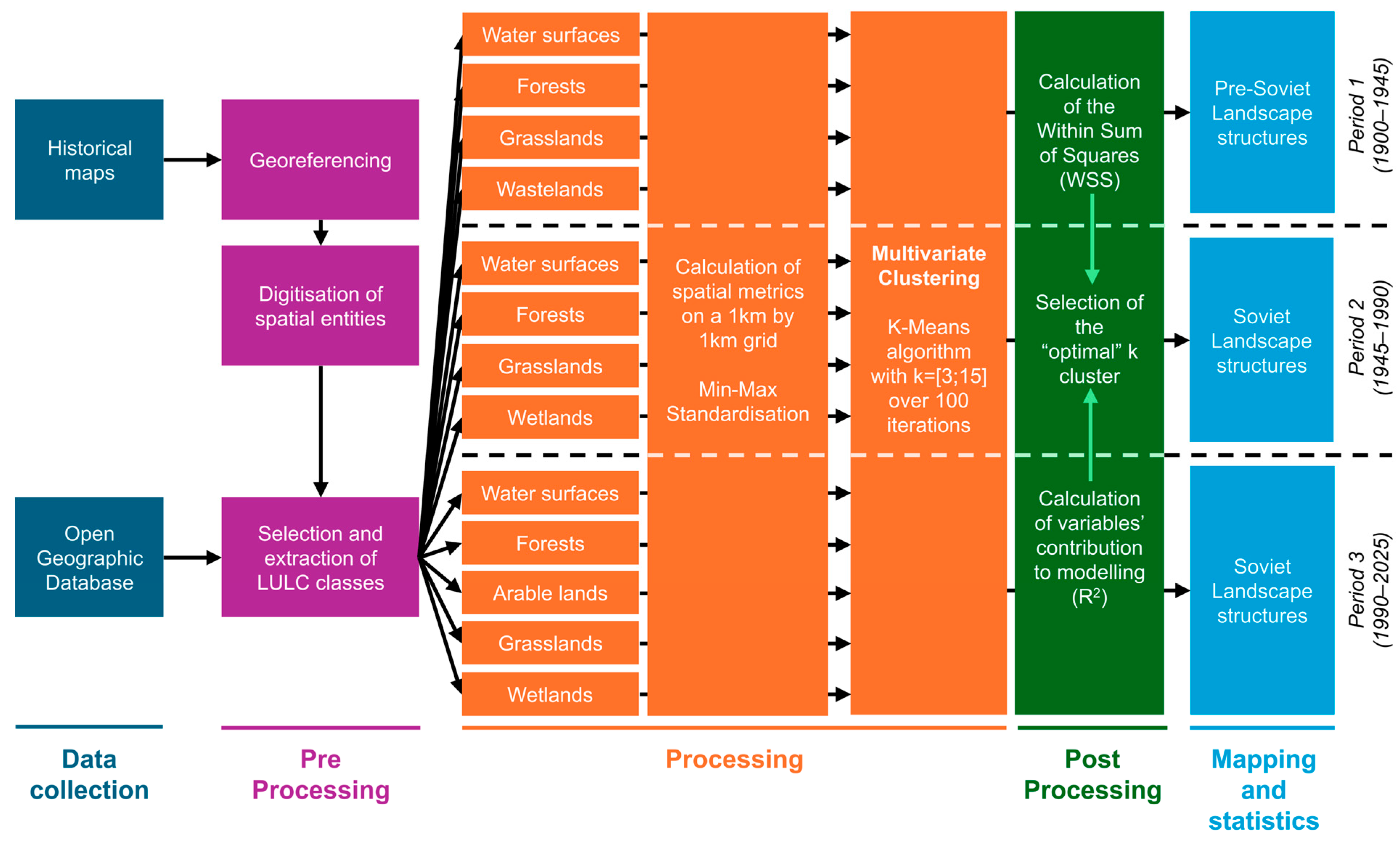
Figure 1 illustrates the methodological approach for modelling the landscape structures of the Lithuanian coastal region, which is further detailed in the following sub-sections through data collection, the application of morphological, configurational, and holistic landscape metrics, and machine-learning multivariate clustering.

The historical analysis is conducted over three distinct periods: the pre-Soviet period (from the beginning of the 20th century until 1945), the Soviet period (from 1945 to 1990), and the post-Soviet period (since 1990).

This choice is justified by the availability of the data needed for the study; the coherence of the historical bifurcations selected, i.e., the political, economic, social, and cultural transformations that are sufficiently significant to produce measurable territorial effects; and the duration of each period (lasting spatial dynamics resulting from major societal bifurcations often emerge only many years later, reflecting the delayed impact of political, economic, and social transformations on territories) [45].

2.1. Data Collection

Land use and land cover data were derived from historical maps and open-access geographic databases (Figure 1). Historical maps were used exclusively for the pre-Soviet and Soviet periods due to their temporal archival value. The main challenge for the pre-Soviet period lies in sourcing data that are both available and consistent in terms of spatial resolution, geographic information, and production dates, particularly between the two areas formerly under the control of the Kingdom of Prussia and the Russian Empire.

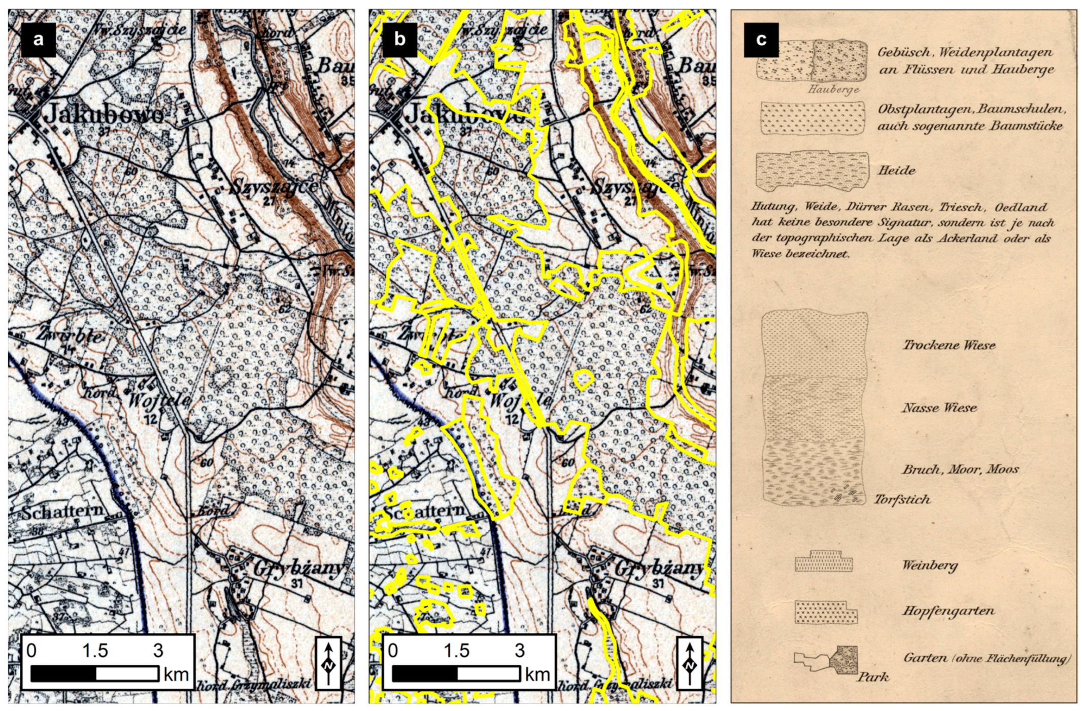
For the Prussian-controlled area, six sheets from the “Karte des Deutschen Reiches” series—dated 1914, 1916, 1917, and 1920—were utilised. This series, produced between 1870 and 1944, offers a monochrome (black and white) resolution of 1:100,000. These maps were complemented by four sheets from the “Karte des Westlichen Russlands” series—dated 1897, 1915, and 1920—produced between 1892 and 1921, which share similar spatial resolution and colour characteristics (an excerpt is shown in Figure 2).

Georeferencing of these historical maps was performed using a set of control points evenly distributed across each sheet, based on identifiable physical features (e.g., road intersections, specific infrastructures, etc.) visible on both the historical maps and modern satellite imagery. A spline transformation method was employed for the georeferencing processing with an average margin of error below 10 m.

For the Soviet period (1945–1990), Soviet military topographic maps were used. Specifically, the 1985 series comprising 24 colour sheets at a spatial resolution of 1:50,000, already georeferenced, was employed.

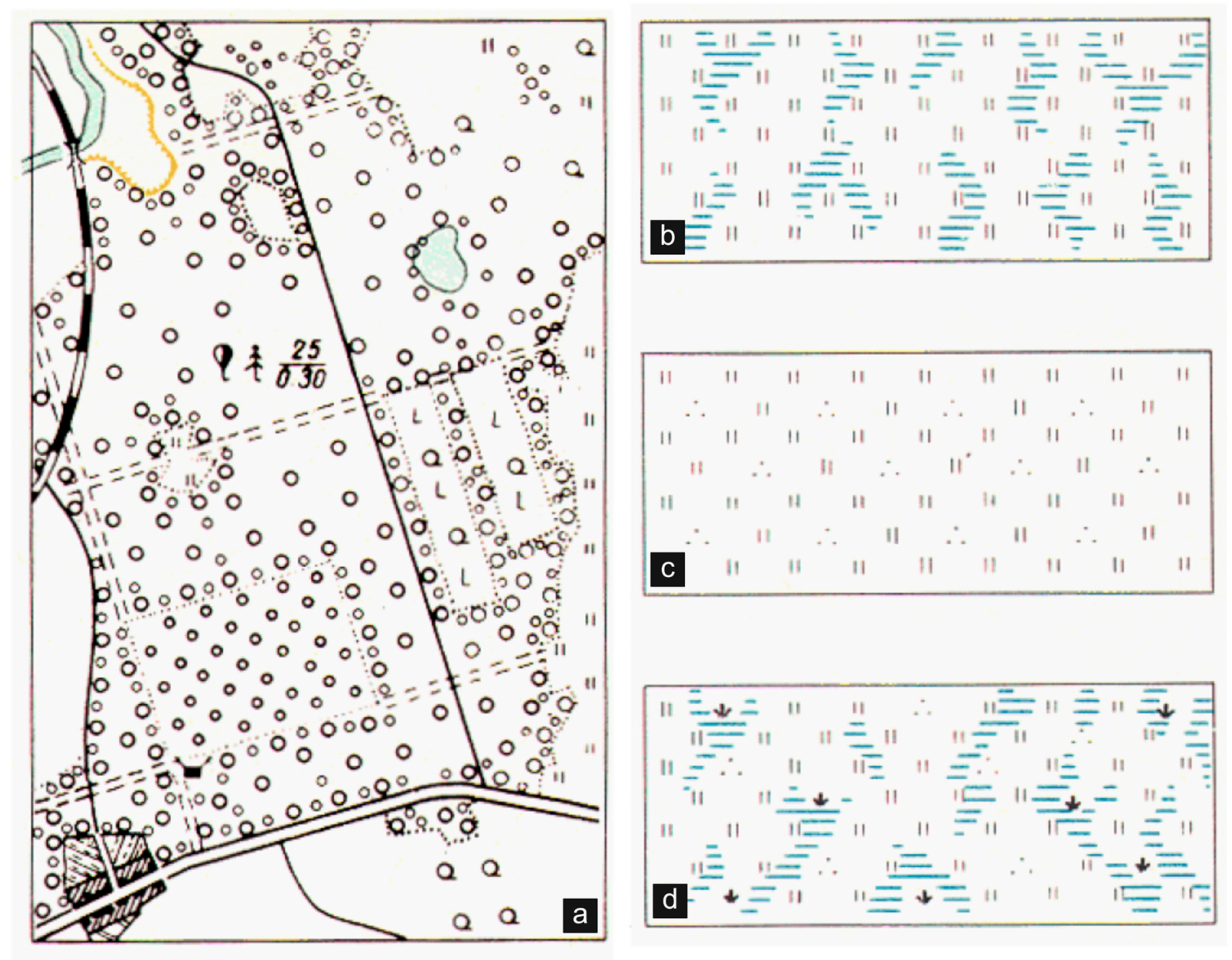
Given the significant variability in scan resolutions (ranging from 100 to 600 dpi), manual digitisation was preferred for extracting spatial entities related to land use and land cover. Each digitised vector feature was classified according to the legend-defined nomenclature (Figure 2). The cartographic sources were produced in diverse historical, institutional, and geopolitical contexts, which present a challenge for the cartographic exploitation of the data [22,23,24]. The nature and hierarchy of the geographical objects represented reflect these contexts and consequently shape the definition of the LULC classes that can be reconstructed from them [46,47]. These data are subject to the interpretation of the operator responsible for digitisation, particularly concerning the visibility of pixels delineating spatial entities related to land use and land cover, the reliability and selection of geographical information represented on the maps, and the assignment of land use and land cover classes to these entities following the established nomenclature [22]. For instance, Soviet military maps often depicted certain features using symbology corresponding simultaneously to multiple land use and land cover classes (Appendix A). In such cases, hybrid classes were created to integrate both dimensions of information.

For the post-Soviet period, the analysis is based on ESA WorldCover data, available at a resolution of 10 m by 10 m [48]. In contrast to historical cartography, this data was produced with the specific purpose of observing land use and land cover.

For each of the three study periods, a preprocessing step involved selecting land use and land cover classes for landscape modelling (Figure 1). This operation led to the identification of classes that were common across all data sources, such as forested areas, water bodies, and grasslands, as well as classes that were specific to sources, including wetlands and wastelands, for example, whose presence was deemed significant in the study area. Artificial surfaces were deliberately excluded from the analysis due to the heterogeneity of their cartographic representation: historical maps primarily depict buildings, whereas more recent sources include zonings that encompass buildings, transport infrastructure, and other man-made structures. A list of the land used and land cover classes, their reclassification, and exclusions is provided in the Appendix A.

2.2. Morphological and Configurational Metrics by Land Use and Land Cover Class to Identify Physical Landscape Structures

Six morphological and configurational metrics—density, shape, size and orientation, spatial cohesion, spatial dispersion, and spatial continuity—are calculated for each digitised entity within the land use and land cover (LULC) classes across the three study periods (Figure 1). These metrics serve to identify and characterise the physical structures of the landscape. To ensure comparability across LULC classes, each index is standardised using min–max normalisation and rescaled to a 0–100 range.

The metrics selected in this study are drawn from disciplines traditionally familiar with landscape analysis, such as ecology, geography, or urban planning, and are frequently applied to a wide variety of contexts: natural, rural, and urban. For example, the shape index, commonly used to describe the circularity or elongation of forest patches or agricultural parcels, can also be applied to urban fabric to characterise urban morphology. This reflects the index’s interdisciplinary applicability and relevance across scales and landscape types. In this sense, the metrics not only support quantitative assessment of landscape structures but also resonate with more classical, typological approaches used in architecture and urban design, such as distinctions of compact vs. dispersed forms, spatial coherence, etc. The objective was to select non-redundant metrics that together provide a comprehensive view of morphological, configurational, and functional aspects.

2.2.1. Density Metric

The first metric quantifies the density of each LULC class within the grid tiles. It is calculated as the ratio between the area occupied by a given class and the total area of the corresponding tile. This index serves to identify areas of high concentration (approaching 100) or dispersion (approaching 0) of specific LULC classes.

2.2.2. Shape Metric

The second metric evaluates the shape of each entity by comparing it to a circular form. Drawing on Gibbs’ work on urban morphology [49], the index is computed by comparing the area of the entity to that of its minimum enclosing circle (Equation (1)):

$$C={\displaystyle \frac{100\times S_E}{\pi \times {\left(\frac{d}{2}\right)}^2}}$$

(1)

• $S_E$: total surface area of the entity.
• $d$: diameter of the circle circumscribing the entity.

Values of the index approaching 0 indicate more elongated shapes, while values nearing 100 correspond to more circular forms. For each tile in the grid, the mean circularity is computed based on the entities it contains. The metric helps distinguish land cover features based on morphological characteristics, for example, differentiating lakes, which tend to be compact or circular, from rivers, which typically display elongated and sinuous shapes.

2.2.3. Size and Orientation Metrics

The third index captures both the size and orientation of features. For each digitised entity within a given LULC class, a standard ellipse is computed based on the spatial distribution of its vertices. The ellipse represents the spatial extent and direction trend of the feature, derived from the standard deviations of the x and y coordinates relative to the feature’s mean centre (Equation (2)) [50].

$${\sigma }_x=\sqrt{{\displaystyle \frac{1}{n}} \sum _{i=1}^n{(x_i-\overline{x})}^2}, {\sigma }_y=\sqrt{{\displaystyle \frac{1}{n}} \sum _{i=1}^n{(y_i-\overline{y})}^2}$$

(2)

• $x_i, y_i$: coordinates of the entity’s vertices.
• $\overline{x}, \overline{y}$: centre of gravity (average of vertices’ coordinates).

Values close to 0 indicate the minimal spatial extent, whereas values approaching 100 represent the maximal extent.

Orientation is determined by the angle of rotation of the standard ellipse relative to the vertical (south–north) axis (Equation (3)) [50]. In the study, an entity oriented towards the east corresponds to a score of 25; towards the south, 50; west, 75; and north, 100. This metric captures the predominant directional alignment of spatial features. The average size and orientation are calculated for each grid tile, considering the features it intersects.

$$\theta ={\displaystyle \frac{1}{2}}{tan}^{-1}\left({\displaystyle \frac{2\times cov(x,y)}{{\sigma }_x^2-{\sigma }_y^2}}\right)$$

(3)

• $x, y$: coordinates of the entity’s vertices.

A comparison of sizes and orientations of features, particularly within agricultural forestry parcels, can offer valuable insights into territorial planning policy strategies, land management models, or the dynamics of landscape transformation such as fragmentation.

In addition, the variances of the standard deviations along the x and y axes, as well as the angles of rotation of the ellipses, are calculated to assess the degree of heterogeneity or homogeneity in the sizes and orientations of features across space. A variance index close to 0 reflects a high degree of uniformity in the sizes and orientations of spatial features, whereas a value near 100 indicates strong heterogeneity. Such variability may stem from natural constraints (e.g., topography, hydrography) or human activities (e.g., agricultural practices, urban development).

2.2.4. Spatial Cohesion Metric

The fourth metric quantifies the spatial cohesion of features within each LULC class. It is calculated from the ratio between the perimeter and surface area of the digitised features (Equation (4)), a common indicator of geometric complexity [51]. This ratio ranges between 0 (highly fragmented, irregular features) and 100 (compact, cohesive features). The average value of this index is calculated for each grid tile, based on the features it contains.

$$K=1-\left({\displaystyle \frac{P_E}{S_E}}\right)$$

(4)

• $P_E$: perimeter of the entity.
• $S_E$: total surface area of the entity.

2.2.5. Spatial Dispersion Metric

The fifth metric evaluates the spatial dispersion of features within each LULC class. It is based on the ratio between the number of features present in each grid tile and the distance to the nearest neighbour. This index is used to characterise the degree of concentration or dispersion of features, considering both their number and their spatial distribution.

In contrast to the density index, which simply quantifies the number of entities relative to the area they occupy, the dispersion index focuses on the count of entities and integrates the proximity between entities, specifically through the distance to the nearest neighbour.

A low average distance between neighbours, coupled with a high number of entities, indicated a high spatial concentration (near 0). Conversely, a high distance between entities suggests significant dispersion (nearly 100). Since the calculation depends on the number of entities per grid tile, the grid resolution can significantly influence the results of the spatial dispersion metric.

2.2.6. Spatial Continuity Metric

The sixth metric quantifies the degree of spatial continuity among entities of the same LULC class within the analysis grid. A tile is considered continuous if it contains at least one entity of the designated class, and if one of its eight neighbouring tiles (first-order Moore neighbourhood) also contains an entity of the same class [52]. The presence of an entity in each adjacent tile signifies the maximal continuity (100).

This index is useful for identifying connected spatial structures, such as ecological corridors, and for detecting large-scale landscape patterns, especially at the territorial scale. However, it is important to note that the value of the index is highly sensitive to the tile size, which may influence the interpretation of the results at different spatial scales.

2.3. Holistic Metrics to Assess Landscape Structures

Two additional metrics—entropy and relief—are computed at the scale of the entire study area for each of the three periods. In contrast to the previous metrics, the entropy index considers the complete set of LULC classes, while the relief index is derived independently of LULC classifications.

2.3.1. Entropy Metric

The entropy metric (Shannon index) quantifies the diversity of LULC classes within each grid tile. It is calculated based on the proportional surface area occupied by each LULC class in the tile [53]. A low entropy value indicates the dominance of a single LULC class (low diversity), whereas a high value reflects a more balanced distribution among multiple classes (high diversity). An index value of 0 denotes complete homogeneity, where only one class is present.

In this analysis, the proportions used in the entropy calculation correspond to the ratio of the area of the class occupied by each class to the total area of the tile. Importantly, all theoretically possible classes are included in the calculation, even those not represented in a given tile, to ensure comparability across tiles by accounting for the full potential structure of the landscape.

2.3.2. Relief Metric

The relief index is derived from the mean elevation of pixels measuring approximately 30 m by 30 m, based on 30 m SRTM (Shuttle Radar Topography Mission) elevation data for each intersecting grid tile [54].

This index remains constant across the three periods studied, as topographic variation is assumed to be negligible at the territorial scale between periods and limited to specific development projects, such as port extension or coastal infrastructure, for example. The relief index is the only metric that was not standardised to a 0–100 scale, as it retains its original values in metres. This is due to the use of the same elevation dataset across all three study periods, ensuring consistency in topographic representation.

Relief is considered a stable contextual variable that helps to interpret its spatial dynamics in the landscape. In the Baltic Eastern region, particularly in Lithuania, the relief is notably flat and exhibits low variability, which can characterise certain landscape structures. Its inclusion enables the identification of patterns potentially shaped by elevation, without being influenced by marginal anthropogenic modifications.

2.4. Machine Learning-Based Multivariate Clustering of Landscape Structures

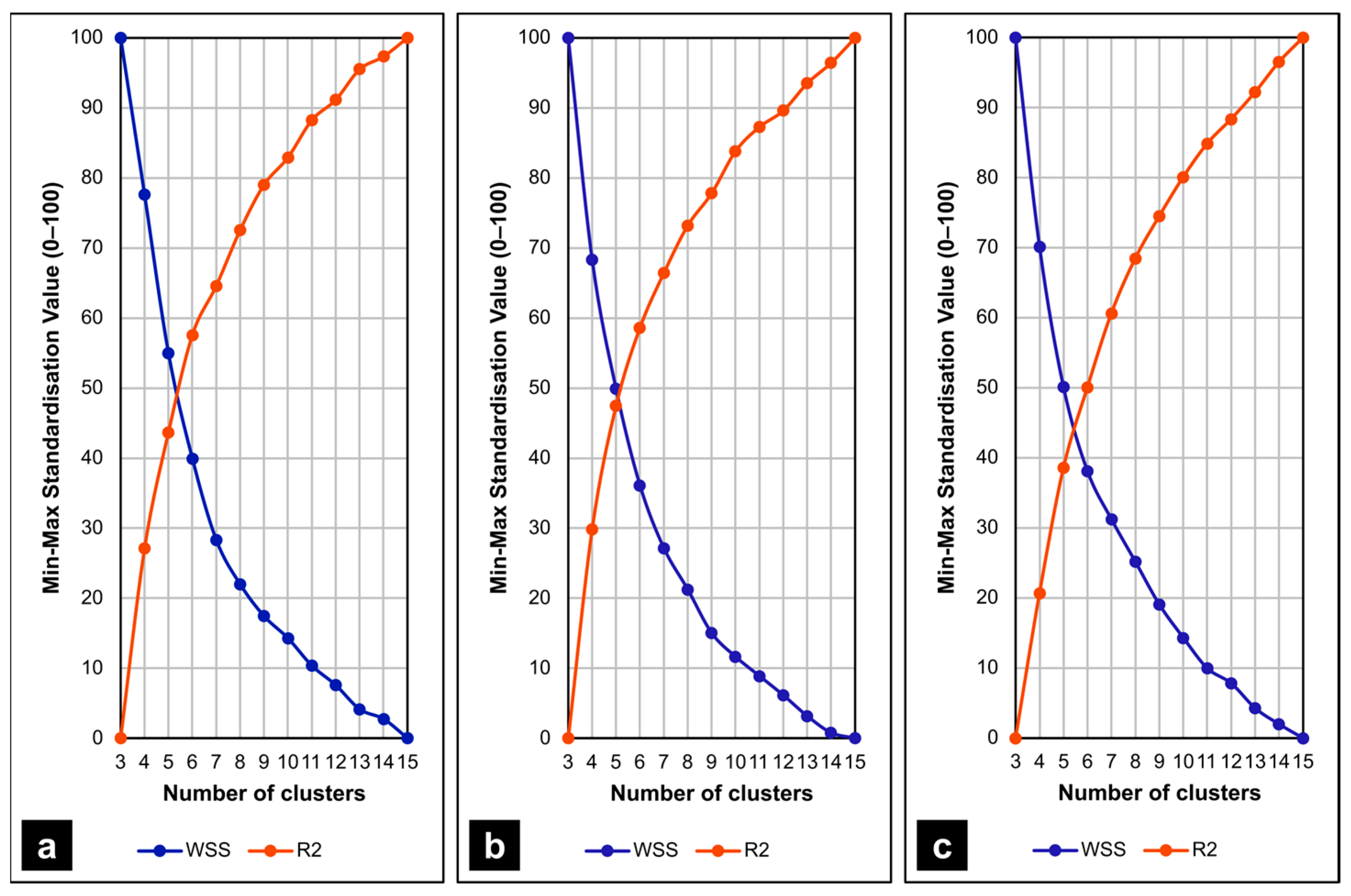
The metrics are calculated on a 1 km-by-1 km grid, a spatial resolution suitable for capturing local and territorial landscape dynamics. Landscape structural modelling is performed using a multivariate clustering approach based on the k-means machine learning algorithm, with the previously computed morphological and configurational metrics serving as explanatory variables (Figure 1). The objective is to group the grid tiles into homogeneous landscape structures (clusters) that minimise intra-cluster variance while maximising inter-cluster variance. An initial estimate of the optimal number of clusters (k) is obtained using the within-cluster sum of squares (WSS), a common metric for assessing cluster compactness [55]. However, in this case, WSS values declined monotonically, rendering the elbow method inconclusive for identifying a clear inflexion point (Figure 3).

To reinforce this cluster selection process, the average contribution of the variables to clustering (R² coefficient) is computed across 100 iterations (given the sensitivity of the k-means algorithm to initial cluster centroid placement) for k values ranging from 3 and 15. Clustering beyond 15 classes is not considered, as higher granularity diminishes the interpretability of results (identification of the main landscape structures). As expected, R² increases with the number of clusters, while the WSS decreases. To reconcile these two opposing trends, both curves are standardised and intersected to determine an optimal balance point between intra-cluster cohesion and inter-cluster separation (Figure 3).

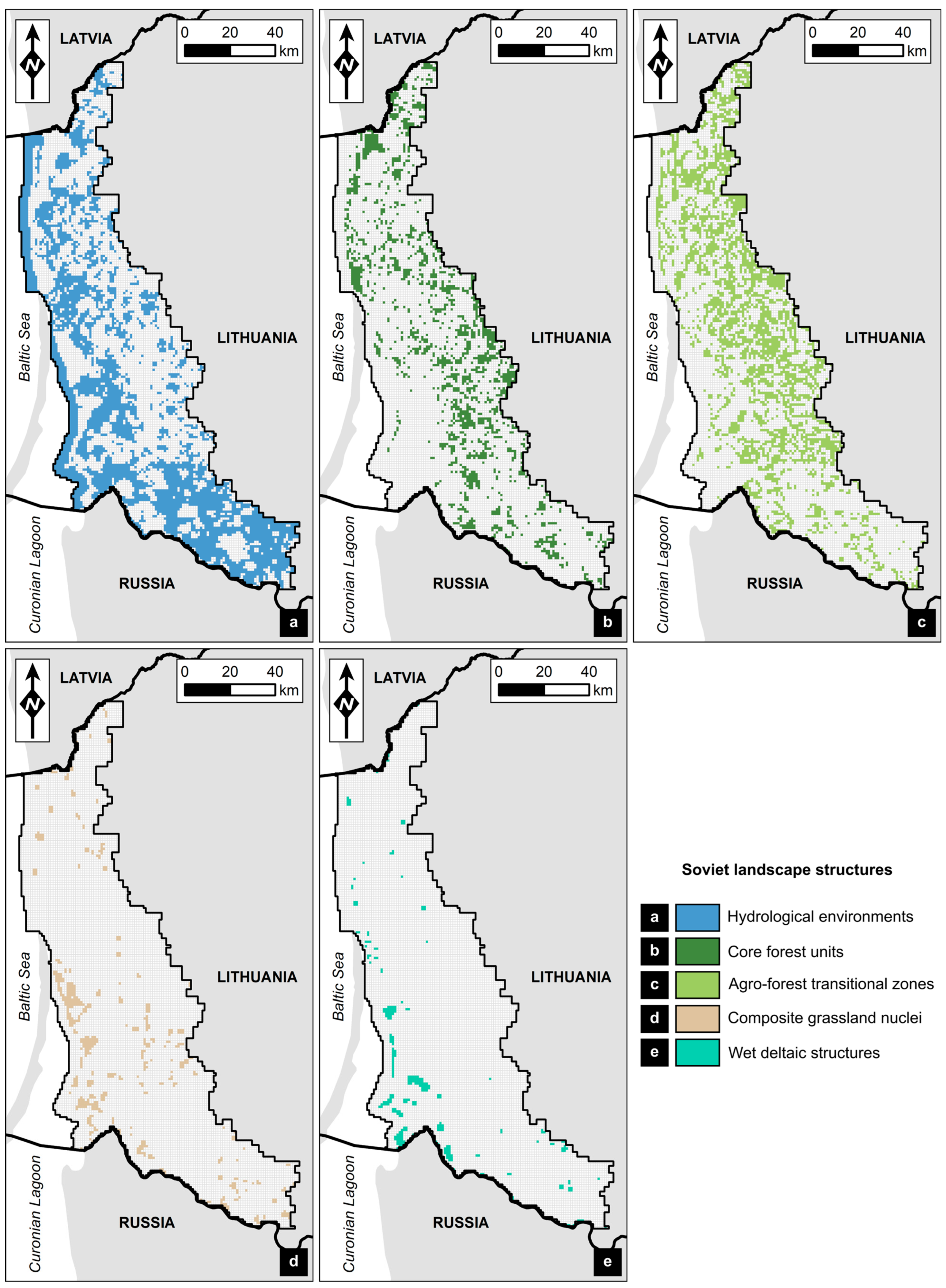
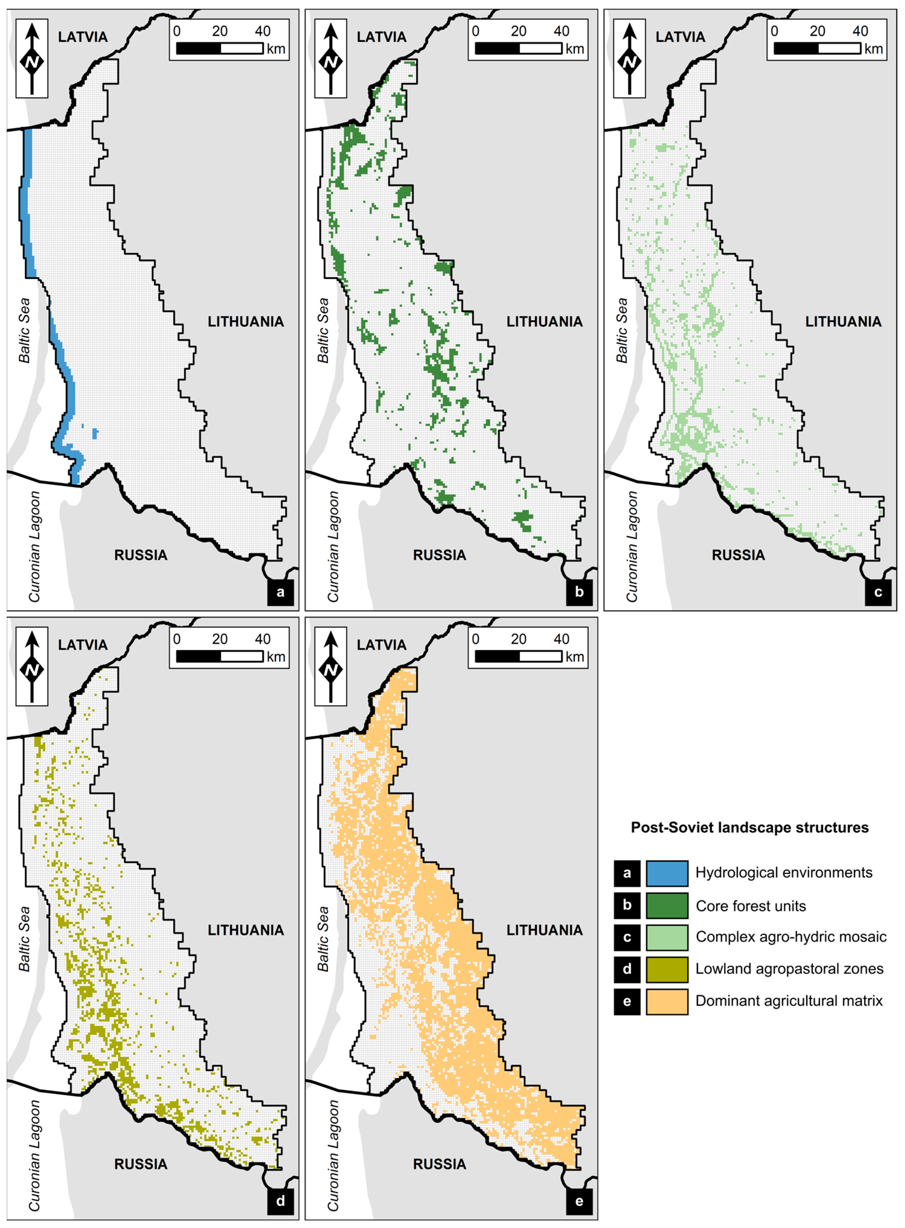
For each of the three periods of study—pre-Soviet, Soviet, and post-Soviet—this method consistently identified five distinct landscape structural clusters. The iteration yielding the highest average R² value, reflecting the optimal explanatory power of the input variables (metrics), was selected for the final analysis.

3. A Diachronic Spatial Analysis of Physical Landscape Structures

The modelling of physical structures of the coastal landscape is presented separately for each study period, due to the variations in LULC classes and differences in data resolution between sources. For each period, the mean metric values (scaled from 0 to 100) for each LULC class are used to characterise the clusters in terms of land use and land cover composition, patch morphology and spatial configuration, as well as entropy and relief-related metrics. The spatial distribution of the clusters is also considered. Each cluster corresponds to a physical landscape structure specific to the given period.

3.1. Typology of Pre-Soviet Landscape (1870–1920)

The modelling of pre-Soviet landscape structures is based on the main LULC classes present in the study area, i.e., water surfaces, forests, meadows, and wastelands. Marginal classes, such as nurseries or sandy areas, were excluded from the analysis due to their low spatial representativeness (Appendix A). The maximum average contribution of the indexes to the modelling was 0.51, reflecting a moderate ability to discriminate between landscape structures based on the variables selected.

3.1.1. Pre-Soviet Hydrological Environments

This landscape structure includes low-relief areas (average relief of 3.33 m) dominated by water surfaces such as the Baltic Sea, Curonian Lagoon, major rivers (Niemen, Minija, Danė), and lakes (Figure 4). The moderate entropy index (16.14) reflects limited land cover diversity, with some localised heterogeneity tiles.

Grasslands exhibit the highest density (47.87), a large patch size (26.90), strongest cohesion (98.87), and low fragmentation (average spatial dispersion of 2.31), making them well-structured and spatially coherent (

Table 1. Averages of spatial metrics for land use and land cover classes in pre-Soviet “Hydrological Environments”.

	Water Surfaces	Forest	Grasslands	Wastelands
Form	5.74	18.39	14.05	17.54
Cohesion	98.56	98.03	98.87	98.22
Continuity	75.85	63.9	85.66	47.70
Density	46.30	20.55	47.87	14.85
Spatial Dispersion	1.75	6.31	2.31	4.68
Size	76.86	10.68	26.90	8.85
Orientation	85.51	53.25	54.98	45.11

).

Forest and wastelands are also present but appear more dispersed, with smaller patch sizes and moderate continuity.

This cluster represents the main hydrological and hydromorphic system composed of water bodies, wet meadows, and scattered shrubby or fallow lands.

3.1.2. Pre-Soviet Core Forest Units

This landscape structure is primarily composed of forest areas, with low land cover diversity (entropy index of 11.53). Forests dominate, though some areas include water bodies and wastelands (

Table 2. Averages of spatial metrics for land use and land cover classes in pre-Soviet “Core Forest Units”.

	Water Surfaces	Forest	Grasslands	Wastelands
Form	19.60	18.54	0.00	15.45
Cohesion	95.64	99.03	0.00	99.18
Continuity	31.71	84.79	0.00	37.50
Density	3.85	52.44	0.00	3.60
Spatial Dispersion	4.72	2.29	0.00	7.24
Size	25.70	28.77	0.00	12.78
Orientation	66.55	54.74	0.00	16.89

).

These forests are mostly located in higher elevation zones (average relief of 31.76 m), especially in the large eastern part of the region, formerly under Russian control, an area showing strong territorial continuity (84.79) (Figure 4). Forest patches here are the most significant (average size of 28.77), dense (52.44), cohesive (99.03), and minimally fragmented (low dispersion of 2.29) (Table 2). While water surfaces and wastelands are marginal (low densities of 3.85 and 3.60), the water bodies tend to be circular (circularity of 19.60), indicating potential features as lakes or ponds. Coastal residual forests are also noted in the former Prussian part of the territory (Figure 4).

3.1.3. Pre-Soviet Agroforest Transitional Zones

This landscape structure represents a hybrid, transitional zone, characterised by forests and grasslands, and a higher land cover diversity (entropy index of 27.05).

Located mainly near forest cores in the eastern, formerly Russian-controlled region, it shares a similar elevation with the forest-dominated cluster (average relief of 28.59 m) (Figure 4). Forest patches here are less dense (29.52) and smaller (17.64), but still cohesive (98.56), with slightly higher dispersion and fragmentation than the forest core cluster (

Table 3. Averages of spatial metrics for land use and land cover classes in pre-Soviet “Agroforest Transitional Zones”.

	Water Surfaces	Forest	Grasslands	Wastelands
Form	14.41	20.47	15.10	11.01
Cohesion	94.01	98.56	98.42	97.34
Continuity	40.53	76.07	78.96	37.50
Density	3.86	29.52	25.47	9.57
Spatial Dispersion	3.93	3.98	5.81	4.78
Size	26.02	17.64	14.37	4.40
Orientation	50.65	50.82	52.28	20.30

).

Grasslands are smaller (14.37), with moderate density (25.47), high cohesion (98.42), but lower territorial continuity (78.96) and greater local dispersion (5.81), suggesting scattered yet structurally coherent patterns (Table 3).

This structurally diverse landscape blends forest and grassland patches that, while coherent at the broader scale, are more fragmented locally, reflecting the dynamic nature of agroforestry systems. Water surfaces and wastelands are minimal (densities of 3.86 and 9.57) (Table 3).

3.1.4. Cohesive Open Grasslands

This landscape structure is defined by open lands dominated by grasslands, with low land cover diversity (entropy index of 9.40) and a moderate elevation (average relief of 20.94 m), indicating gently undulating terrain.

This is the most spatially diffuse cluster with scattered patches over almost the entire study area, with the exception of the Niemen delta and its adjacent territory to the east (Figure 4).

Grasslands here show a high patch density (36.93), moderate size (19.00), strong cohesion (98.53), and higher dispersion (4.77), suggesting scattered but territorially coherent structures (

Table 4. Averages of spatial metrics for land use and land cover classes in pre-Soviet “Cohesive Open Grasslands”.

	Water Surfaces	Forest	Grasslands	Wastelands
Form	0.34	0.00	15.12	0.00
Cohesion	90.52	0.00	98.53	0.00
Continuity	25.00	0.00	84.32	0.00
Density	1.05	0.00	36.93	0.00
Spatial Dispersion	2.38	0.00	4.77	0.00
Size	9.96	0.00	19.00	0.00
Orientation	11.59	0.00	51.17	0.00

).

Unlike the hydromorphic cluster, this structure consists almost exclusively of grasslands. Despite some local fragmentation, high territorial continuity (84.32) indicated a well-connected grassland pattern across the broader landscape, typical of open, homogeneous environments.

3.1.5. Marginal and Altered Lands

This cluster is dominated by wastelands, with moderate land cover diversity (entropy index of 22.80). Grasslands and water surfaces are present but marginal.

Located mainly in the Niemen River plain and some coastal areas, it has a low elevation (average relief of 12.69 m) (Figure 4).

Wastelands show the highest density (39.80) and a significant patch size (34.92), exceeding that of forests and grasslands. Water areas are fewer in number (density of 7.43) but have the largest average patch size (40.17), influenced by the proximity of the Niemen River and deltaic aquatic formations (

Table 5. Averages of spatial metrics for land use and land cover classes in pre-Soviet “Marginal and Altered Lands”.

	Water Surfaces	Forest	Grasslands	Wastelands
Form	15.66	21.59	14.85	20.98
Cohesion	96.03	98.07	96.94	99.15
Continuity	41.71	64.51	72.68	71.24
Density	7.43	19.90	23.82	39.80
Spatial Dispersion	4.16	6.79	6.70	5.25
Size	40.17	10.71	15.42	34.92
Orientation	74.15	52.72	53.75	53.42

).

This cluster is marked by low territorial continuity and high spatial dispersion across all LULC types, reflecting fragmented, degraded, and structurally incoherent landscapes. Typically situated on the periphery of more structured areas, these zones represent low-dynamism, underutilised or environmentally altered lands.

3.2. Typology of Soviet Landscape (1985)

The modelling of Soviet landscape structures is based on LULC classes, some of which are identical to those of the pre-Soviet period, such as water surfaces and forests. Conversely, the large number of detailed classes related to herbaceous and wet formations (e.g., shrub, reed swamp, reed and grass, etc.) has been grouped into two main categories: grasslands and wetlands (Appendix A). The maximum average contribution of the variables to the model is comparable to that obtained for the pre-Soviet period, with a value of 0.51.

3.2.1. Soviet Hydrological Environments

Similar to the pre-Soviet model, this landscape structure is characterised by a dominance of water bodies. The low entropy index (4.39) reflects strong LULC homogeneity primarily due to the dominance of aquatic features.

While the relief is low (average of 13.85 m), it is higher than in the pre-Soviet hydrological cluster, as it includes inland water bodies like rivers, lakes, and irrigation canals, rather than being limited to the sea and lagoon (Figure 5). As a result, this cluster now spans the broader former Prussian territory, with more dispersed but still cohesive aquatic nuclei, especially in the Niemen plain.

Water surfaces here show moderate density (22.76), but are generally significant in size, spatially close (dispersion of 2.44), minimally fragmented (cohesion of 95.28), and highly continuous (84.11), indicating a structured and connected hydrological system across sea, lagoon, and inland waterways (

Table 6. Averages of spatial metrics for land use and land cover classes in Soviet “Hydrological Environments”.

	Water Surfaces	Forest	Grasslands	Wetlands
Form	3.40	0.00	0.00	0.00
Cohesion	95.28	0.00	0.00	0.00
Continuity	84.11	0.00	0.00	0.00
Density	22.76	0.00	0.00	0.00
Spatial Dispersion	2.44	0.00	0.00	0.00
Size	55.74	0.00	0.00	0.00
Orientation	68.96	0.00	0.00	0.00

).

3.2.2. Soviet Core Forest Units

This cluster, consistent with the pre-Soviet period, is dominated by forests, with a low land cover diversity (entropy index of 12.90) and minimal presence of water surfaces (density of 0.39) (

Table 7. Averages of spatial metrics for land use and land cover classes in Soviet “Core Forest Units”.

	Water Surfaces	Forest	Grasslands	Wetlands
Form	0.84	20.33	0.00	0.00
Cohesion	88.61	98.56	0.00	0.00
Continuity	12.50	84.43	0.00	0.00
Density	0.39	45.85	0.00	0.00
Spatial Dispersion	0.00	3.72	0.00	0.00
Size	2.33	25.51	0.00	0.00
Orientation	7.15	52.45	0.00	0.00

).

It features the highest elevation in the region (average relief of 31.41 m), with forest areas concentrated in upland zones. Structurally, the forests remain similar to those of the earlier period: moderately sized patches (25.51), high density (45.85), strong territorial continuity (84.43), and low spatial dispersion, indicating cohesive and continuous forest cover with limited fragmentation (Figure 5).

3.2.3. Soviet Agroforest Transitional Zones

This landscape structure reflects a transitional landscape between forest and agricultural land, similar to the pre-Soviet agroforestry structure, characterised by forests and water surfaces, with relatively high land cover diversity (entropy mean of 22.36).

It spans a large portion of the study area, especially the former Russian-controlled region, excluding the Niemen plain and its western delta (Figure 5). Forest patches are less dense (31.84), smaller (18.25), and slightly more dispersed (4.00) than in core forest areas, though still highly cohesive (98.46), indicating moderate fragmentation (

Table 8. Averages of spatial metrics for land use and land cover classes in Soviet “Agroforest Transitional Zones”.

	Water Surfaces	Forest	Grasslands	Wetlands
Form	4.14	20.78	0.00	0.00
Cohesion	93.23	98.46	0.00	0.00
Continuity	73.54	76.47	0.00	0.00
Density	4.94	31.84	0.00	0.00
Spatial Dispersion	4.12	4.00	0.00	0.00
Size	31.76	18.25	0.00	0.00
Orientation	61.08	49.74	0.00	0.00

).

Water bodies are more residual, with low density (4.94), medium-sized patches (31.76) and reduced cohesion (93.23) and continuity (73.54) compared to the main hydrological structure (Table 8).

Unlike the pre-Soviet period, meadows are no longer prominent, making this a forest–agriculture transitional zone shaped more by woodland and water infrastructure (irrigation canals that likely serve adjacent arable lands) rather than by grasslands.

3.2.4. Composite Grassland Nuclei

This landscape structure is notably different from pre-Soviet typologies, characterised by a strong presence of grasslands, secondary forest presence, and marginal water bodies. The high entropy index (27.27) confirms this heterogeneous land cover pattern.

Grasslands show a moderate density (21.66) and patch size (24.03) but exhibit high local dispersion (8.54), with weak territorial continuity (49.88), indicating isolated and scattered clusters (Figure 5,

Table 9. Averages of spatial metrics for land use and land cover classes in Soviet “Composite Grassland Nuclei”.

	Water Surfaces	Forest	Grasslands	Wetlands
Form	4.70	19.44	18.10	9.48
Cohesion	95.92	98.73	98.32	68.76
Continuity	77.94	81.03	49.88	0.00
Density	15.51	39.98	21.66	0.11
Spatial Dispersion	2.65	3.17	8.54	10.12
Size	57.19	25.72	24.03	0.07
Orientation	69.85	54.42	53.22	0.81

). Despite this, their spatial cohesion remains high (98.32).

Forests have a high density (39.98) and size (25.72), with relatively low dispersion (3.17) and strong territorial continuity, resembling core forest structures in coherence but differing in context (Table 9).

Water surfaces are residual but include large patches (57.19), low dispersion (2.65), and moderate continuity (77.94), reflecting scattered but cohesive aquatic areas, especially in coastal lagoon areas (Figure 5).

This is a spatially fragmented and mixed structure, predominantly grassland-based, with significant internal variability and patchy landscape connectivity.

3.2.5. Wet Deltaic Structures

The landscape structure can be described as a deltaic wetland mosaic, characterised by the dominance of wetlands and a high diversity of LULC classes, as reflected by an elevated entropy index (average of 22.36). Located in low-lying areas (average elevation of 5.42 m), especially in the Niemen delta and along the Curonian Lagoon, this structure reflects the complexity of deltaic environments (Figure 5).

Wetland areas exhibit the highest patch density (average of 23.25), with moderate average patch sizes (28.86) and the highest levels of spatial dispersion across all LULC types (average of 9.33). These characteristics point to a highly fragmented distribution at the local scale, accompanied by limited territorial continuity (average of 47.29), indicating the presence of isolated and weakly connected wetland units (

Table 10. Averages of spatial metrics for land use and land cover classes in Soviet “Wet Deltaic Structures”.

	Water Surfaces	Forest	Grasslands	Wetlands
Form	7.07	19.17	13.71	19.30
Cohesion	95.69	98.23	98.18	98.16
Continuity	81.12	74.29	53.14	47.29
Density	18.31	26.77	21.81	23.25
Spatial Dispersion	2.65	4.51	2.70	9.33
Size	55.77	15.35	26.16	28.86
Orientation	68.13	54.37	44.97	52.37

).

Grasslands, though less dominant, show a similar patch size (26.16) and moderate density (21.81), marked by high local cohesion (98.18) but limited continuity across the territory (53.14) (Table 10).

Water surfaces are less frequent (density of 18.30) but from large, well-connected patches (average size of 55.77 and average continuity of 81.12), often adjacent to major aquatic systems (Table 10).

Forest, only marginally present, is defined by modest densities (26.77), small patch sizes (15.35), and moderate territorial cohesion (74.29) (Table 10).

Overall, this structure is shaped by a dispersed and heterogeneous configuration, with multiple land cover types intersecting in a fragmented yet ecologically significant, deltaic landscape. However, the spatial distribution of this landscape structure remains limited in the study area (Figure 5).

3.3. Typology of Post-Soviet Landscape (2021)

The modelling of landscape structures in the post-Soviet period is predicated on the primary LULC classes present in the designated study area, namely water surfaces, forests, meadows, and wetlands, as well as, specifically for this period, arable land. In contrast to the previous models, this model explicitly incorporates cultivated farmland. The maximum average contribution of the indexes to the modelling is 0.45, which reflects the moderate capacity of the variables selected to discriminate between landscape structures.

3.3.1. Post-Soviet Hydrological Environments

The first cluster corresponds to the coastal hydrological landscape, largely centred on the Baltic Sea, the Curonian Lagoon, and the aquatic systems of the Niemen delta, resembling the spatial configuration observed during the pre-Soviet period (Figure 6). The structure is dominated by water surfaces, as confirmed by a very low entropy index (average of 0.47), indicating minimal land cover diversity.

The relief index (average of −0.03 m) confirms the extremely low elevation of these areas, consistent with their coastal and deltaic nature. Water patches are exceptionally large (average size of 83.34) and dense (99.62), forming a nearly continuous matrix with negligible spatial dispersion and very high levels of spatial cohesion (99.81) and territorial continuity (99.62) (

Table 11. Averages of spatial metrics for land use and land cover classes in Post-Soviet “Hydrological Environments”.

	Water Surfaces	Forest	Grasslands	Wetlands	Arable Land
Form	4.25	11.30	11.56	11.07	30.65
Cohesion	99.81	96.06	92.75	96.52	40.55
Continuity	99.62	47.50	45.00	57.50	25.00
Density	99.49	0.73	2.61	6.92	0.02
Spatial Dispers.	0.00	0.66	0.58	0.47	26.14
Size	83.34	38.93	5.87	26.13	0.00
Orientation	94.10	23.35	41.89	57.32	95.67

).

Other LULC classes, such as arable land (mean density of 0.02), forest (0.73), grassland (2.61), and wetland (6.92), appear only marginally, mainly along the coastal interface, highlighting the structural dominance and spatial integrity of aquatic environments.

3.3.2. Post-Soviet Core Forest Units

The second landscape structure corresponds to forest-dominated areas, as in previous periods. Forest cover is the only LULC, while the moderate entropy index (12.18) reflects limited land cover diversity.

Forest patches are large (average of 45.04) and dense (87.54), forming cohesive and compact areas. This is supported by very high spatial cohesion (98.91), strong territorial continuity (98.40), and minimal spatial dispersion (0.24) (

Table 12. Averages of spatial metrics for land use and land cover classes in Post-Soviet “Core Forest Units”.

	Water Surfaces	Forest	Grasslands	Wetlands	Arable Land
Form	16.58	15.28	22.16	25.66	20.06
Cohesion	86.88	98.91	91.70	73.01	86.41
Continuity	51.79	98.40	93.36	34.38	59.00
Density	19.11	87.54	9.89	1.10	2.79
Spatial Dispers.	4.40	0.24	4.41	5.23	1.64
Size	29.53	45.04	2.87	0.85	5.17
Orientation	71.56	48.40	53.54	48.42	36.02

).

These forests are mainly located along the northern coastline, between Gargždai and Šilutė, with some occurrences on the Niemen plain and in inland northern zones (Figure 6). Their location on regional hilltops is reflected in the highest average elevation among clusters (27.41 m).

Water surfaces are also present, with notable density (19.11) and a moderate patch size (29.53), though they show higher dispersion (4.40), lower continuity (51.79), and reduced cohesion (86.88) compared to forests. These likely represent sea surfaces intersecting coastal forest tiles (Table 12).

Other LULC types remain marginal: wetlands (average density of 1.10), arable land (2.79), and grasslands (9.89).

3.3.3. Complex Ago-Hydric Mosaic

The third landscape structure corresponds to heterogeneous wet arbustive meadow patches, echoing a similar pre-Soviet configuration. It combines multiple LULC types with wetlands, water surfaces, grasslands, and forests and is marked by high entropy (47.07), reflecting strong land cover diversity.

Located primarily in the lowlands of the Nemunas Delta (average elevation of 7.47 m), this structure features small, dispersed wetland patches (density of 12.17, size of 2.08, continuity of 65.54) (Figure 6,

Table 13. Averages of spatial metrics for land use and land cover classes in Post-Soviet “Complex Ago-Hydric Mosaic”.

	Water Surfaces	Forest	Grasslands	Wetlands	Arable Land
Form	20.84	21.12	22.30	23.48	25.70
Cohesion	86.53	94.66	95.92	83.69	60.90
Continuity	54.10	86.09	95.54	65.54	85.40
Density	10.92	23.83	39.74	12.17	15.16
Spatial Dispers.	2.69	2.11	0.44	2.08	1.47
Size	12.09	7.32	7.14	3.37	3.18
Orientation	60.07	52.51	57.18	59.34	60.04

).

Grasslands are more cohesive (density of 39.74, cohesion of 95.92, and continuity of 95.54), while forests, though less extensive (density of 23.83 and size of 7.32), are also well-structured spatially (cohesion of 94.66) (Table 13).

This cluster forms a transitional agro-wetland mosaic of diverse, small-scale patches, combining dense grasslands and forest elements with fragmented aquatic features.

3.3.4. Lowland Agropastoral Zones

The fourth landscape structure represents an agropastoral zone dominated by wetlands, grasslands, and arable lands, with moderate diversity indicated by an entropy index of 33.26. Situated mainly in low-lying coastal zones of the southwest study area and the Niemen plain (average relief of 7.19 m), this cluster includes some residual nuclei in the northern part of the region (Figure 6).

Wetlands are relatively sparse and fragmented, with low density (7.70), small patches (2.50), higher spatial dispersion (4.21), and moderate cohesion (77.27) and continuity (57.83). Grasslands are more dominant and cohesive, exhibiting high density (50.64), larger patches (12.65), strong spatial coherence (96.46), and territorial connectivity (99.35). Arable lands show a moderate density (26.20) and patch size (5.16), with low dispersion but higher fragmentation (cohesion of 63.95) compared to other classes (

Table 14. Averages of spatial metrics for land use and land cover classes in Post-Soviet “Lowland Agropastoral Zones”.

	Water Surfaces	Forest	Grasslands	Wetlands	Arable Land
Form	10.57	22.59	21.66	25.70	25.22
Cohesion	88.35	94.32	96.46	77.27	63.95
Continuity	75.00	85.49	99.35	57.83	91.48
Density	0.23	22.05	50.64	7.70	26.20
Spatial Dispers.	0.09	3.64	0.34	4.21	0.98
Size	0.47	8.21	12.65	2.50	5.16
Orientation	12.34	51.51	58.74	61.91	58.80

).

This cluster typifies agropastoral areas where extensive, well-connected grasslands are interspersed with smaller arable fields and scattered wetland remnants.

3.3.5. Dominant Agricultural Matrix

The final landscape structure represents a predominantly agricultural matrix, distinguished by the dominance of arable land, accompanied by smaller proportions of grassland and marginal woodland. The entropy index (35.54) indicates moderate land cover heterogeneity despite the arable land predominance. This cluster is generally located on slightly elevated terrain (average elevation of 26.83 m), mainly along the eastern study area border, with compact nuclei in the east and more dispersed patches toward the west (Figure 6).

Arable land patches are relatively larger compared to the other clusters (average size of 10.53) and densely concentrated (density of 39.36), showing local dispersion (0.58) and strong territorial connectivity (93.31), though spatial coherence is moderate (67.12), possibly due to internal fragmentation or sub-parcelling. Grasslands are dense (35.87), with smaller, compact patches (7.34) displaying high coherence (95.38) and continuity (99.02) (

Table 15. Averages of spatial metrics for land use and land cover classes in Post-Soviet “Dominant Agricultural Matrix”.

	Water Surfaces	Forest	Grasslands	Wetlands	Arable Land
Form	25.44	22.16	23.18	0.00	24.02
Cohesion	77.37	95.29	95.83	0.00	67.12
Continuity	28.00	89.48	99.02	0.00	93.31
Density	1.89	25.81	35.87	0.00	39.36
Spatial Dispers.	9.88	3.06	0.55	0.00	0.58
Size	3.19	12.74	7.34	0.00	10.53
Orientation	59.03	53.96	57.44	0.00	57.90

). Forest remnants, though less abundant, have a moderate density (25.81) and relatively large patches (12.74), with average spatial metrics reflecting well-structured but somewhat scattered woodlands integrated into the agricultural matrix (Table 15).

4. Immutability and Structural Dynamics of Coastal Landscape Structures

Although the source data present incomplete and heterogeneous land use and land cover classifications, a relative stability in landscape composition can be observed over the 125-year study period (Figure 7). This stability is inferred from the presence of a consistent composition across the three periods analysed. In particular, three landscape structures appear especially persistent: (1) the hydrological network, which retains a consistent spatial framework, (2) forest cores, representing stable land cover entities over time, and (3) agricultural land use, despite the absence of explicit arable land classes in the earlier historical maps but deduced from other classes. A fourth, more localised and partially constrained structure relates to natural or semi-natural areas such as wetlands and wastelands.

While these four structures show relative stability in terms of land use and land cover composition, their internal structure evolves under the influence of political, economic, social, and cultural dynamics.

4.1. A Dual Influence of the Maritime and Lagoon Environments and the River Systems

One of the structures consistently identified across the three study periods corresponds to the hydrological network. This recurrent pattern can be attributed to the combined influence of the maritime and lagoon environments—namely, the Baltic Sea and the Curonian Lagoon—and the river systems, with the Niemen River and its delta being the most prominent components (Figure 7).

This primary hydrological structure can, however, be partially dissociated, as water surfaces are also present in other, more composite landscape structures, particularly those associated with meadows. In these cases, water surfaces, though less dominant, still contribute to a landscape characterised by a diversified and mixed spatial configuration.

The spatial extent of the main hydrological structure varied over time. During the Soviet era, the hydrological network expanded significantly beyond its primary maritime and fluvial core, covering a much larger share of the territory (Figure 5a and Figure 7b). This expansion likely reflects the cartographic conventions of the era, which placed a greater emphasis on irrigation and drainage infrastructures implemented for agricultural modernisation. These changes can be understood as a manifestation of the broader transformation of rural landscapes initiated by collectivisation policies from the 1940s onwards.

It is reasonable to assume that the number of clusters in the model would allow for a finer distinction between the maritime hydrological component and its terrestrial counterpart, thereby improving the identification of intensively irrigated agricultural zones during the Soviet period without necessarily having a class relating to arable land. Irrigation and drainage networks are responsible for a reduction in natural vegetation as well as a decrease in the diversity of land cover classes [56].

Post-Soviet modelling does not capture the full terrestrial extent of these networks due to the spatial resolution of the data, which does not allow for the detection of features smaller than 100 m²—this being the case for most networks here. Moreover, these drainage systems have been heavily degraded with time, with some no longer functional and in need of restoration [57].

4.2. Temporal Persistence and Transformation of Forest Core Structure

The second sustainable landscape structure identified over time corresponds to forested areas, primarily located along the eastern border of the study region (Figure 7). It comprises a series of forest cores, among which the most prominent are the coastal forests (in the north of Klaipėda and near Palanga), as well as the Šilutė and Pagegiai forests on the Niemen River plain.

Beyond these stable forest areas, the location or spatial extent of forest cores varies substantially across the studied periods. These fluctuations are mainly due to differences in LULC classification across modelling iterations, where certain wooded areas may, at times, be integrated into more heterogeneous landscape structures, and at others reassigned to a dedicated forest cluster.

During the pre-Soviet period, the forest structure was characterised by geographical compactness and relative homogeneity, traits even more pronounced when transitional agroforestry zones are included. This configuration partly overlaps with the former territory of the Russian Empire (Figure 4b,c and Figure 7a), suggesting distinct cultural approaches to land use between areas under Prussian and Russian influence. The higher forest density in the Russian-administered zone may reflect a lower degree of agricultural intensification. This hypothesis is supported by historical maps that show the persistence of linear street villages typical of the medieval Teutonic period, still widespread at the beginning of the 20th century [45,58]. At that time, agrarian reforms promoting individual and family farming—already underway in much of Europe—had not yet been widely implemented in the Russian Empire, with the Stolypin reform dating only from 1906. The maps used date back to 1920 at the most. It was only after Lithuania’s independence of 1918 that these changes gradually took effect for the entire study region [2].

Although the forest core structure was generally preserved during the Soviet period, it appears more diffuse and fragmented for similar morphological and configurational characteristics with the pre-Soviet period forest structure (although these results should be compared with the utmost caution given the heterogeneity of the data) (Figure 5b and Figure 7b). As previously discussed, the land collectivisation reforms introduced in Lithuania from the 1940s led to the dismantling of numerous family farms. In certain cases, the abandonment or reallocation of agricultural land may have facilitated processes of spontaneous or state-led reforestation on unused plots [59]. Similarly, the development of irrigation and drainage canals, and ultimately the expansion of agriculture, may have contributed to fragmentation in other areas.

In the post-Soviet period, the configuration of forest cores—and more broadly, of less dense and smaller forest formations—becomes more complex to delineate (Figure 6b and Figure 7c). These areas are frequently embedded in mixed landscape structures alongside other LULC classes, such as arable land (Table 15), complicating their clear identification. Nevertheless, a tendency toward a reduction in the number of large, discrete forest cores can be observed (Figure 6b), with the remaining ones forming more compact clusters. The post-Soviet landscape did not undergo a uniform regression, but rather a structural transformation, reflecting a coexistence of dynamics including fragmentation, spontaneous regeneration, and the reallocation of land use functions. This interpretation is supported by the results of remote sensing analysis from the same period, which highlight an increase in forest cover in the Klaipėda district [43,60].

4.3. Temporal Variability and Ambiguity of Landscapes Shaped by Extensive and Intensive Agricultural Practices

Several identified structures are dominated by grassland, often wet or semi-wet in character. During the pre-Soviet period, these grasslands occupied a large portion of the northern half of the territory, particularly in what was formerly East Prussia (Figure 4d and Figure 7a). Although arable land is not explicitly represented in the LULC data from this period, agricultural activities were likely well-established in this part of the territory. This assumption aligns with the agrarian reforms aimed at individualising land ownership that began in the late 19th century. Supporting this interpretation are the sociocultural characteristics of the local population, especially the “Lietuvininkai” (Prussian Lithuanians), a Protestant group that traditionally placed a strong emphasis on private land ownership, education, and agricultural productivity [61,62]. This is also reflected in the spatial structure of settlements, with dispersed, autonomous farms prevalent in this region.

In contrast, during the Soviet period, grassland-dominated structures became marginal and were mainly restricted to the southwestern end of the study area, particularly in the Niemen delta (Figure 5d and Figure 7b). This shift can be explained by several intersecting factors. First, the collectivisation reforms initiated in the 1940s brought about profound changes in rural organisation. The subsequent intensification of agriculture likely led to the progressive conversion of grasslands into arable land [56]. This hypothesis is supported by the observation of a linear trend of grassland decline ranging from 0 to −3% between 1971 and 1990 [35].

Additionally, the Soviet maps used in this study may reflect a different approach to vegetation classification. Unlike earlier or contemporary cartographic representations, Soviet maps seldom depict grasslands as a distinct, homogeneous category. Instead, grassland-related cover types are often subdivided into more hybrid categories, such as grassland with sparse woodland, herbaceous marshland with shrubs, mixed marshland with reeds and woody elements, etc. This typological and terminological diversity reflects the practical orientation of Soviet cartography, which served military and agricultural planning purposes. As a result, grasslands—especially when fragmented or peripheral—were often subsumed under other LULC categories. This practice likely led to an under-representation of grasslands in Soviet datasets and complicated comparisons across periods.

Recent data reveal that arable land currently dominates much of the study zone, whether in relatively homogeneous or more diversified landscape structures (Figure 6e and Figure 7c). This highlights the historical association of the notion of “landscape” in Lithuania with agrarian functions in rural areas [45]. However, the modelling also seems to reflect a subtler and less visible phenomenon: the gradual abandonment of agricultural land.

The decline of agricultural surfaces appears to be part of a broader structural change affecting the region’s socio-economic and territorial organisation. It reflects both a declining interest in agricultural activities and the difficulties of maintaining them, particularly in the aftermath of the post-Soviet and restitution process [63]. These transformations are expressed in the emergence of more mixed LULC configurations, where arable land coexists with other classes, such as forests and grasslands. This stands in contrast to earlier periods when agricultural areas could be more easily identified due to the less diversified landscape structure, with open agricultural plains in the pre-Soviet era and clearly defined irrigated networks during the Soviet period, making interpretation more straightforward.

The increasing diversity of LULC classes within these structures may therefore both obscure and reveal the decline of agriculture in the post-Soviet period: it conceals it by integrating it into more composite configurations but also reflects it by signalling a loss of coherence and dominance of traditional agricultural land uses.

4.4. The Niemen Delta: From Traditional Use to Protected Wetland Landscape

Several mixed structures characterise natural or semi-natural landscapes that are largely influenced by the Niemen River in a small part of the study area. These semi-natural landscapes are made up of meadows, wastelands, and wetlands, consistently identified in the three steps of modelling (Figure 7). These conditions may have led to the establishment of specific rural traditional communities, with fishermen and farmers living in the peat bogs and wet meadows, whose way of life is essentially dictated by the river and flooding cycle, preventing any intensive farming [58]. These communities were widespread during the pre-Soviet period but were largely dismantled by Soviet policies of collectivisation and village/population consolidation. As a result, these landscapes have remained under the dominant influence of natural features. Today, this region has become a Ramsar-protected wetland and is part of the Natura 2000 European network, aimed at conserving and protecting natural ecosystems. The area is now characterised by a low population density, which has helped preserve the ecological integrity of the Niemen delta. The modelling has repeatedly underscored the role of the Niemen delta in shaping the spatial configuration of certain LULC classes within broader landscape structures.

4.5. Critical Analysis of Landscape Structural Modelling

Two important aspects related to the retrospective modelling of landscape structures deserve particular attention.

The spatial ontology-based approach adopted in this study enabled the identification of structural changes by highlighting morphological and configurational variations, thereby going beyond potential differences in the interpretation of land use and land cover classes. However, it does not resolve the persistent issue of source data completeness. Nevertheless, by associating classes and inferring missing elements, certain structures could be deduced and interpreted. The clearest example concerns agricultural plots: although not explicitly represented in historical maps, they were indirectly considered in the analysis through the presence of irrigation/drainage canals and the detection of grassland areas.

The second issue relates to the robustness of explanatory variables underlying the structural model. Their average contribution proved relatively modest (R² = 0.49). This invites reflection on the choice of metrics, which were deliberately limited to avoid redundancy and balanced across functional, morphological, and configurational dimensions. However, they may have lacked the specificity or sensitivity needed to capture the full complexity of landscape structures.

The modelling algorithm may also be questioned. K-means clustering, originally sensitive to raw data variance, might have overemphasised certain variations while underestimating others. Moreover, metrics were computed separately by land use and land cover classes, potentially limiting the model’s ability to identify coherent groupings, as the likelihood of divergent clustering increases with the number of metrics.

Weighting mechanisms could have enhanced the model, for instance, by considering the spatial extent of land cover classes and assigning less importance to those with limited surface area. Similarly, weighting based on the reliability of underlying datasets could reinforce the modelling process. Yet, such improvements often require auxiliary datasets to cross-validate historical information, which are not always available.

Deep learning algorithms may offer an alternative by modelling latent relationships and handling part of the inherent complexity of spatial structures.

Considering that landscapes are a component of broader spatial systems, part of the observed structures should integrate additional data, such as networks and built environments, as key structuring elements.

Finally, one hypothesis worth considering is that some of the modelling noise may stem from the absence of pre-existing structure (before the analysed period) in the model, even though it continues to influence observed spatial configurations.

These considerations open up interesting avenues for improving the reconstruction and interpretation of historical landscape structures.

5. Conclusions and Perspectives

The objective of this research is to analyse the evolution of landscape structures in the coastal region of Klaipėda, Lithuania, over 125 years. Relying on historical geospatial data from digitised maps and open-access databases, morphological and configurational metrics are applied to major land use and land cover classes. These were subsequently modelled using a multivariate machine-learning-based clustering method.

The results suggest that despite classification limitations, consistent patterns in landscape organisation can be identified through spatial reasoning, cross-class inference, and structural metrics. Five main landscape structures are identified across the pre-Soviet, Soviet, and post-Soviet periods. After a detailed examination of their spatial distribution, along with metric averages, an important aspect emerging from this research is the identification of persistent landscape structures across the pre-Soviet, Soviet, and post-Soviet periods. These enduring patterns, despite undergoing internal reconfiguration, suggest a form of evolutionary continuity that coexists with more abrupt, policy-driven transformations, or “revolutions” in land use and landscape organisation.

The identified structures were primarily shaped by the influence of hydrological systems (Baltic Sea, Curonian Lagoon, and main rivers), the extent and transitional dynamics of forest cover, the varying intensity of agricultural activity—from extensive grassland to intensive arable farming—and the persistence of natural and semi-natural environments, such as wetlands and wastelands.

Through their spatial distribution and configurational patterns, this study highlights the societal dynamics that influence their evolution, including the role of cultural factors in shaping territorial organisation. In particular, it highlights the contrast between the former Prussian territories, marked by open grasslands and pre-industrial farming practices, and the former Russian-controlled areas, where forest has remained dominant. The Niemen delta also emerged as a distinct landscape, shaped by its unique functions, spatial organisation, and environment.

A second key finding relates to the extensive transformations driven by Soviet land collectivisation policies. These are visible through the widespread irrigation networks established to modernise agriculture, the significant reduction in grasslands previously associated with extensive farming, and the fragmentation and expansion of forest cover, likely reflecting reforestation processes following land abandonment.

This study also highlighted post-Soviet transformations, particularly the abandonment of agricultural land due to declining interest in agriculture and the challenges of reappropriating land within the structural legacy of Soviet collectivisation. Compared to the more distinct agrarian landscapes of earlier periods, the post-Soviet agricultural landscape appears more fragmented and heterogeneous (mixed landscape structures).

One of the main findings of this study is that landscape transformations are predominantly structured around agricultural dynamics. The impacts of collectivisation policies, post-Soviet land restitution, and agrarian reforms promoting farm individualisation emerge as major drivers of change. Although the analysis was limited by the incomplete availability of data for this specific land use class, the centrality of agriculture in shaping territorial organisation is evident. This observation reinforces the strong rural identity associated with the landscape [45].

It is important to mention that this study primarily focused on analysing anthropogenic dynamics, but part of the evolution of landscape structures can also be explained by natural dynamics.

The combination of morphological and configurational metrics and machine-learning-based clustering offers a significant enhancement to traditional landscape classification approaches. This method allows for a data-driven, reproducible, and quantitative characterisation of landscape structures. It captures not only land cover composition but also spatial configuration, enabling the detection of patterns that might otherwise remain hidden in aggregated or visually interpreted classifications. This approach facilitates a more granular understanding of landscape heterogeneity and evolution, supporting cross-period comparisons despite heterogeneous source data (spatial resolution, land use and land cover classifications).

References

1. Plakans, A. A Concise History of the Baltic States; Cambridge University Press: Cambridge, UK, 2011; pp. 215–448. [Google Scholar]
2. Jespen, M.R.; Kuemmerle, T.; Müller, D.; Erb, K.; Verburg, P.H.; Haberl, H.; Vesterager, J.P.; Andrič, M.; Antrop, M.; Austrheim, G.; et al. Transitions in European Land Management Regimes between 1800 and 2010. Land Use Policy 2015, 49, 53–64. [Google Scholar]
3. Ragauskaitė, A. Ethnocultural regionalisation of Lithuania or all the truth about our regions. Acta Museol. Lith. 2019, 4, 162–168. [Google Scholar]
4. Idzelis, A. Industrialisation and population change in the Baltic republics. Lituanus 1984, 30, 26–42. [Google Scholar]
5. Vaitkus, G.; Vaitkuvienė, D. Land cover changes in the Lithuanian coastal zone during 1975–2000. Acta Zool. Litu. 2005, 75, 183–187. [Google Scholar] [CrossRef]
6. Köll, A.M. Reinterpretation of economic history in the Baltic countries, 30 years after independence. Scand. Econ. Hist. Rev. 2024, 73, 93–102. [Google Scholar] [CrossRef]
7. Ubarevičienė, R.; van Ham, R. Population decline in Lithuania: Who lives in declining regions, and who leaves? Reg. Stud. Reg. Sci. 2017, 4, 57–79. [Google Scholar] [CrossRef]
8. Veteikis, D.; Šabanovas, S.; Jankauskaitė, M. Landscape structure changes on the coastal plain of Lithuania during 1998–2009. Baltica 2011, 24, 107–116. [Google Scholar]
9. Cirtautas, M. Changing periphery of the Baltic cities: Lithuanian case. J. Archit. Urban. 2015, 39, 56–69. [Google Scholar] [CrossRef]
10. Anandkumar, A.; Vijith, H.; Nagarajan, R.; Jonathan, M.P. Evaluation of Decadal Shoreline Changes in the Coastal Region of Miri, Sarawak, Malaysia. In Coastal Management; Academic Press: Cambridge, MA, USA; Elsevier: Amsterdam, The Netherlands, 2019; pp. 95–119. [Google Scholar]
11. Favory, F.; Van der Leeuw, S. Archaeomedes, la durabilité des systèmes spatiaux. In Des Oppida aux Métropoles; Economica Anthropos: Paris, France, 1998; pp. 13–44. [Google Scholar]
12. Allain, R. Formes urbaines et paysages urbains. In Morphologie Urbaine. Géographie, Aménagement et Architecture de la Ville; Armand Colin: Paris, France, 2004; pp. 9–24. [Google Scholar]
13. Jones, M.; Olwig, K. Thinking Landscape and Regional Belonging on the Northern Edge of Europe. In Nordic Landscapes. Region and Belonging on the Northern Edge of Europe; University of Minnesota Press: Minneapolis, MN, USA, 2008; pp. ix–xxix. [Google Scholar]
14. Gosme, C. Landscape. Hypergéo. 2005. Available online: https://hypergeo.eu/landscape/?lang=en (accessed on 12 May 2025).
15. García-Díez, V.; García-Llorente, M.; González, J.A. Participatory Mapping of Cultural Ecosystem Services in Madrid: Insights for Landscape Planning. Land 2020, 9, 244. [Google Scholar] [CrossRef]
16. Kivinen, S.; Vartiainen, K.; Kumpula, T. People and Post-Mining Environments: PPGIS Mapping of Landscape Values, Knowledge Needs, and Future Perspectives in Northern Finland. Land 2018, 7, 151. [Google Scholar] [CrossRef]
17. Claval, P. Géographie Culturelle, Culture des Géographes. Géoconfluences. 2003. Available online: https://geoconfluences.ens-lyon.fr/informations-scientifiques/dossiers-thematiques/remue-meninges/paul-claval (accessed on 12 May 2025).
18. Fedorov, G.M.; Mikhailov, A.S.; Kuznetsova, T. The influence of the sea on the economic development and settlement structure in the Baltic Sea Region. Balt. Reg. 2017, 9, 4–18. [Google Scholar] [CrossRef]
19. Druzhinin, A.; Gontar, N.; Mikhaylov, A. Population Dynamics in the Coastal Urban Settlements of the Baltic Sea Region. J. Settl. Spat. Plan. 2019, 10, 61–70. [Google Scholar] [CrossRef]
20. Escach, N. Réseaux de Villes et Recompositions Interterritoriales Dans L’espace Baltique. Ph.D. Thesis, École Normale Supérieure, Lyon, France, 2014. [Google Scholar]
21. Lévy, J.; Lussault, M. Dictionnaire de la Géographie et de L’espace des Sociétés; Belin: Paris, France, 2013; pp. 852–854. [Google Scholar]
22. Kaim, D.; Kozak, J.; Ostafin, K.; Dobosz, M.; Ostapowicz, K.; Kolecka, N.; Gimmi, U. Uncertainty in Historical Land-Use Reconstructions with Topographic Maps. Quaest. Geogr. 2014, 33, 55–63. [Google Scholar] [CrossRef]
23. Piškinaitė, E.; Veteikis, D. The results of digitising historical maps: Comparison of Lithuanian land-use structure in the 19th and 21st centuries. Land 2023, 12, 946. [Google Scholar] [CrossRef]
24. Piškinaitė, E.; Veteikis, D. Methodologies and prospects of historical land use/land cover studies in Lithuania. Baltica 2022, 35, 60–70. [Google Scholar] [CrossRef]
25. Mushtaq, F.; O’Brien, C.D.; Parslow, P.; Åhlin, M.; Di Gregorio, A.; Latham, J.S.; Henry, M. Land Cover and Land Use Ontology—Evolution of International Standards, Challenges, and Opportunities. Land 2024, 13, 1202. [Google Scholar] [CrossRef]
26. Levin, G.; Groom, G.; Svenningsen, S.R. Assessing spatially explicit long-term landscape dynamics based on automated production of land category layers from Danish late nineteenth-century topographic maps in comparison with contemporary maps. Environ. Monit. Assess. 2025, 197, 195. [Google Scholar] [CrossRef]
27. Farmer, E.; Brewer, T.R.; Sannier, C.A.D. Land cover attributed and their utility within land cover mapping: A practical example. J. Land Use Sci. 2010, 7, 35–49. [Google Scholar] [CrossRef]
28. Claramunt, C. Ontologies for geospatial information: Progress and challenges ahead. J. Spat. Inf. Sci. 2020, 20, 35–41. [Google Scholar] [CrossRef]
29. Nedd, R.; Light, K.; Owens, M.; James, N.; Johnson, E.; Anandhi, A. A Synthesis of Land Use/Land Cover Studies: Definitions, Classification Systems, Meta-Studies, Challenges and Knowledge Gaps on a Global Landscape. Land 2021, 10, 994. [Google Scholar] [CrossRef]
30. Comber, A.; Fisher, P. What is land cover? Environ. Plan. B Plan. Des. 2005, 32, 199–209. [Google Scholar] [CrossRef]
31. Kremsa, V.Š. Sustainable management of agricultural resources (agricultural crops and animals). In Sustainable Resource Management: Modern Approaches and Contexts; Elsevier: Amsterdam, The Netherlands, 2021; pp. 99–145. [Google Scholar]
32. Şenol, H.İ.; Kaya, Y.; Yiğit, A.Y.; Yakar, M. Extraction and geospatial analysis of the Hersek Lagoon shoreline with Sentinel-2 satellite data. Surv. Rev. 2023, 56, 367–382. [Google Scholar] [CrossRef]
33. Gadal, S.; Gloaguen, T. Performance of Landsat 8 OLI and Sentinel 2 MSI Images Based on MNF Versus PCA Algorithms and Convolution Operators for Automatic Lithuanian Coastline Extraction. SN Comput. Sci. 2024, 5, 308. [Google Scholar] [CrossRef]
34. Bauža, D.; Baužienė, I. Evaluation of landscape changes in Lithuania in the second half of the 20th century. Geografija 2008, 44, 28–35. [Google Scholar]
35. Juknelienė, D.; Kaznavičiūtė, V.; Valčiukienė, J.; Atkocevičienė, V.; Mozgeris, G. Spatiotemporal patterns of land-use changes in Lithuania. Land 2021, 10, 619. [Google Scholar] [CrossRef]
36. Tiškutė-Memgaudienė, D. Changes of forest land cover in Lithuania during the period 1950–2017: A comparative analysis. Res. Rural Dev. 2021, 36, 274–279. [Google Scholar]
37. Ivavičiūtė, G. The change of natural landscape in Lithuania. Res. Rural Dev. 2020, 35, 213–218. [Google Scholar]
38. Feranec, J.; Soukup, T.; Taff, G.N.; Stych, P.; Bicik, I. Overview of changes in land use and land cover in Eastern Europe. In Land-Cover and Land-Use Changes in Eastern Europe After the Collapse of the Soviet Union in 1991; Springer: Cham, Switzerland, 2016; pp. 13–34. [Google Scholar]
39. Galinienė, J. Change in Land Use and Land Cover of Lithuanian Coastal Zone: Classification Methods Comparison and Assessment. Ph.D. Thesis, Klaipėda University, Klaipėda, Lithuania, 2020. [Google Scholar]
40. Juknelienė, D.; Narmontienė, V.; Valčiukienė, J.; Mozgeris, G. Driving Forces of Agricultural Land Abandonment: A Lithuanian Case. Land 2025, 14, 899. [Google Scholar] [CrossRef]
41. Gozdowski, D.; Žukovskis, J.; Kaziukonytė, K.; Razinkovas-Baziukas, A. Evaluation of Land Cover Changes in Southwestern Lithuania from 1984 to 2018 Using Medium Spatial Resolution Satellite Imagery. Pol. J. Environ. Stud. 2020, 29, 4041–4051. [Google Scholar] [CrossRef]
42. Sinkevičiūtė, V. Analysis of farming usage in Southern Lithuania. Balt. Surv. 2014, 1, 20–25. [Google Scholar]
43. Lekavičiūtė, J.; Gadal, S. Forest Cover Changes during 1974–2005 in the Lithuanian Coastal Region. In Proceedings of the Fourth International Scientific Conference Rural Development 2009, Kaunas, Lithuania, 15–17 October 2009; Volume 4, pp. 241–247. [Google Scholar]
44. Tercan, E.; Dereli, M.A. Development of a land suitability model for citrus cultivation using GIS and multi-criteria assessment techniques in Antalya province of Turkey. Ecol. Indic. 2020, 117, 106549. [Google Scholar] [CrossRef]
45. Bučas, J. Lietuvos kaimo kraštovaizdžio permainos ir savastis. In Krašto Tvarkos Pagrindai; Technologija: Kaunas, Lithuania, 2001; pp. 109–193. [Google Scholar]
46. David Rumsey Map Collection. Königlich-Preussische Landesaufnahme oder Landvermessungsbehörden. Zeichen-Erklaerung für die Karte des Deutschen Reiches; David Rumsey Map Collection: Stanford, CA, USA, 1887. [Google Scholar]
47. U.S. Department of the Army. Soviet Topographic Map Symbols; U.S. Government Printing Office: Washington, DC, USA, 1958. [Google Scholar]
48. Zanaga, D.; van de Kerchove, R.; Daems, D.; de Keersmaecker, W.; Brockmann, C.; Kirches, G.; Wevers, J.; Cartus, O.; Santoro, M.; Fritz, S.; et al. ESA WorldCover 10 m 2021 v200; Zenodo: Meyrin, Switzerland, 2022. [Google Scholar] [CrossRef]
49. Gibbs, J.P. A Method for Comparing the Spatial Shapes of Urban Units. In Urban Research Methods; D. Van Nostrand: Princeton, NJ, USA, 1961; pp. 99–106. [Google Scholar]
50. Yuill, R.S. The standard deviational ellipse, an updated tool for spatial description. Geogr. Ann. 1971, 53, 28–39. [Google Scholar] [CrossRef]
51. McGarigal, K.; Cushman, S.A.; Ene, E. FRAGSTATS v4: Spatial Pattern Analysis Program for Categorical Maps. 2023. Available online: https://www.fragstats.org/index.php (accessed on 12 May 2025).
52. Moore, E.F. The Shortest Path through a Maze. In Proceedings of the International Symposium on the Theory of Switching, Part II; Harvard University Press: Cambridge, MA, USA, 1959; pp. 285–292. [Google Scholar]
53. Turner, M.G. Landscape ecology: The effect of pattern on process. Annu. Rev. Ecol. Syst. 1989, 20, 171–197. [Google Scholar] [CrossRef]
54. NASA Shuttle Radar Topography Mission (SRTM). Shuttle Radar Topography Mission (SRTM) Global. 2013. Available online: https://www.usgs.gov/centers/eros/science/usgs-eros-archive-digital-elevation-shuttle-radar-topography-mission-srtm (accessed on 12 May 2025).
55. MacQueen, J.B. Some methods for classification and analysis of multivariate observation. In Proceedings of the Fifth Berkeley Symposium on Mathematical Statistics and Probability, Volume 1: Statistics; University of California Press: Berkeley, CA, USA, 1967; Volume 5, pp. 281–298. [Google Scholar]
56. Povilaitis, A.; Lamsodis, R.; Bastienė, N.; Rudzianskaitė, A.; Misevičienė, S.; Miseckaitė, O.; Gužys, S.; Baigys, G.; Grybauskienė, V.; Balevičius, G. Agricultural drainage in Lithuania: Review of practices and environmental effects. Acta Agric. Scand. Sect. B Soil Plant Sci. 2015, 65, 14–29. [Google Scholar] [CrossRef]
57. Klaipėdos Rajono Savivaldybė. Potvynių Prevencijai—Investicijos į Melioracijos Sistemas. 2023. Available online: https://klaipedos-r.lt/potvyniu-prevencijai-investicijos-i-melioracijos-sistemas/ (accessed on 20 June 2025).
58. Atkocevičienė, V.; Valčiukienė, J.; Juknelienė, D.; Agintaitė-Kirstukienė, K. Analysis of the 20th century villages in Nemunas Delta Regional Park. Balt. Surv. Int. Sci. J. 2016, 2, 15–22. [Google Scholar]
59. Zundė, P. The collectivisation of Lithuanian agriculture (1940–1952). Lituanus 1963, 9, 82–88. [Google Scholar]
60. Ivavičiūtė, G. The changes of forest area in Klaipėda county during the period between 2005–2019. J. Balt. Surv. 2020, 12, 8–13. [Google Scholar] [CrossRef]
61. Vareikis, V. Memellander/Klaipėdiškiai Identity and German-Lithuanian Relations in Lithuania Minor in the Nineteenth and Twentieth centuries. Sociol. Mintisi Ir Veiksmas 2001, 6, 54–65. [Google Scholar] [CrossRef]
62. Levchenkov, A.V.; Gumenyuk, I.S. The spatial development of the rural settlement of East Prussia: Kaliningrad region. Int. J. Econ. Financ. Issues 2015, 5, 30–36. [Google Scholar]
63. Sujetovienė, G.; Dabašinskas, G. Ecosystem Service Value Changes in Response to Land Use Dynamics in Lithuania. Land 2023, 12, 2151. [Google Scholar] [CrossRef]
Figure 1. Methodological diagram of the different processing methods used to model landscape structures in the Lithuanian coastal region over 125 years.
Land 14 01356 g001
Figure 2. Preprocessing of historical maps for modelling landscape structures: (a) extract of the “Schattern–Korciany” sheet (1914) from the 1:100,000 Karte des Deutsche Reiches series after georeferencing, (b) digitisation process of spatial features relating to land use and land cover, and (c) extract of the nomenclature [46] for identifying land use and land cover classes.
Land 14 01356 g002
Figure 3. Trends in the standardised (min–max) within-cluster sum of squares (WSS) and the average contributions of the variables to clustering (R2 coefficient) for 3 to 15 clusters over the (a) pre-Soviet, (b) Soviet, and (c) post-Soviet periods.
Land 14 01356 g003
Figure 4. Spatial distribution of the pre-Soviet landscape structures with (a) hydrological environments, (b) core forest units, (c) agro-forest transitional zones, (d) cohesive open grasslands, and (e) marginal and altered lands.
Land 14 01356 g004
Figure 5. Spatial distribution of the Soviet landscape structures with (a) hydrological environments, (b) core forest units, (c) agro-forest transitional zones, (d) composite grassland nuclei, and (e) wet deltaic structures.
Land 14 01356 g005
Figure 6. Spatial distribution of the post-Soviet structures with (a) hydrological environments, (b) core forest units, (c) complex agro-hydric mosaic, (d) lowland agropastoral zones, and (e) dominant agricultural matrix.
Land 14 01356 g006
Figure 7. Spatial distribution of landscape structures for the (a) pre-Soviet, (b) Soviet, and (c) post-Soviet periods.
Land 14 01356 g007