Bridging Heritage Systems: Multi-Scale Spatial Coupling Between Tangible and Intangible Cultural Heritage in China Using Hierarchical Bayesian Model and Causal Inference

Abstract

Cultural heritage systems play a crucial role in decoding human–environment interactions and social evolution. This study aims to reveal the spatial coupling characteristics of tangible and intangible cultural heritage in China, as well as the heterogeneity of their driving mechanisms. After quantifying heritage coupling at three geographic scales, we integrated a hierarchical Bayesian model with a hybrid causal inference framework to identify the correlations, causal effects, and heterogeneity of the driving factors. The empirical results indicate the following: (1) The coupling patterns exhibit scale dependence. The proportion of strongly coupled areas decreases from the prefecture-level scale to the provincial scale but increases at the cultural–geographical unit scale. This suggests that China’s cultural system has a cohesive effect that transcends administrative boundaries. (2) The hierarchical Bayesian model identifies the significant effects of mean annual temperature, population density, GDP–population interaction, transport–hydrological network interaction, and industrial structure. Effect strengths generally peak at the prefecture-level scale and decrease at the provincial scale. (3) Causal inference estimates the causal effects of mean annual temperature, transport–hydrological network interaction, mean annual precipitation, and water network density on coupling. (4) Heterogeneity tests reveal that the positive causal effect of transport–hydrological network interaction and the negative causal effect of mean annual precipitation are significant only in low-temperature regions. By integrating hierarchical modeling with causal verification, this study elucidates the mechanisms underlying heritage coupling. This provides a scientific basis for understanding the spatial patterns of cultural heritage systems and formulating differentiated conservation policies.

1. Introduction

As carriers of human history and civilization, cultural heritage embodies the collective memory of nations and serves as a bridge connecting the past and present. China’s symbiotic system of tangible (TCH) and intangible (ICH) cultural heritage provides valuable insights into cultural evolution on a global scale [1]. TCH represents the material imprints that document historical processes, while ICH perpetuates cultural traditions in living practice. The Convention Concerning the Protection of the World Cultural and Natural Heritage and the Convention for the Safeguarding of the Intangible Cultural Heritage have, respectively, established international normative frameworks for TCH and ICH. However, their separate structures have led to persistent integration challenges in policy-making and management practices [2]. Scholars have increasingly employed perspectives such as the assemblage theory [3] to critically reflect on this binary framework, conceptualizing heritage as a dynamically evolving system composed of material spaces, social actors, institutions, and cultural practices [4]. By examining the spatial interactions and structural logics among elements and incorporating comprehensive systems of culture and nature, this research field has developed the theory of heritage systems, which is characterized by fuzzy boundaries and value associations [5,6].

In this study, heritage systems are defined as multi-level evolutionary systems encompassing material remains, living practices, and spatial environments, which are embedded within broader natural and socio-economic systems. Their systemic boundaries are generated across regional and local scales. TCH and ICH interact through spatial proximity and cultural processes to form interconnected subsystems that constitute complementary relational networks. Despite its limitations, the binary TCH–ICH framework is still employed as an analytical tool due to the methodological and normative advantages of official inventory systems. These inventories provide heritage datasets with clearly defined spatial boundaries, ensuring regional comparability, value assessment criteria, and institutional frameworks, which facilitate the identification of factors influencing coupling patterns within heritage systems. In other words, using the official system serves to test, rather than perpetuate, the binary classification model and analyze the value judgments and cultural processes embedded within this institutional component. The research objective is to reveal the dynamic processes and synergistic relationships obscured by this framework through empirical methods [7], thereby transcending the static classification logic that treats the two heritage types as mutually independent entities. This contributes to understanding the spatial association patterns and driving mechanisms between them, providing a scientific basis for formulating adaptive conservation strategies.

From the perspective of cultural geography, cultural landscapes represent the manifestation of cultural relationships within the material environment [8], and long-term interactions between space and culture provide a theoretical basis for understanding heritage distribution. Within this framework, heritage is conceptualized as cultural elements that aggregate, diffuse and co-locate within specific territories. Their formation processes reflect the ongoing evolution of social practices, local identities and social networks [9]. Previous studies have indicated that, although TCH and ICH are institutionally categorized as distinct types, they often exhibit functionally complementary and spatially intertwined relationships in practice [10]. This interrelation provides a critical theoretical foundation for understanding the coupling patterns between the two heritage types based on heritage pattern analysis. Recent research on the spatial aspects of cultural heritage has become increasingly interdisciplinary [11,12], primarily focusing on distribution patterns and influencing factors. Scholars have commonly employed methods such as kernel density estimation [13], standard deviational ellipses [14], and nearest-neighbor indices [15] to analyze clustering characteristics and spatiotemporal patterns across multiple geographic scales, including the national [16], watershed [17], provincial [18], and municipal levels [19]. Within frameworks that encompass natural [20], social [21], and cultural factors [22], quantitative approaches—such as decision trees [23], geographic detectors [24], and geographically weighted regression [25]—have also become popular for elucidating underlying mechanisms. However, two systematic gaps remain in the field. Firstly, TCH and ICH are frequently considered separately [1], often lacking analysis of their spatial coupling. Only a few studies have examined the coupled interactions between heritage and external systems, such as tourism [26], urbanization, or cultural transmission [27], while the internal coupling between TCH and ICH has received limited attention. Secondly, from a methodological perspective, traditional statistical approaches struggle to address the high dimensionality, nonlinearity, and heterogeneity inherent [28] to heritage data. While some machine learning models can capture complex patterns, their limited interpretability [29] restricts their ability to provide causal evidence to inform heritage policy. In particular, the driving mechanisms of coupling may vary across spatial scales, posing challenges for cross-scale heterogeneity analyses.

To address these research gaps, this study focuses on the spatial coupling patterns between TCH and ICH in China, as well as the heterogeneity of their driving mechanisms. The research aims to identify the characteristics of heritage association networks in different regions, and to examine how social and natural factors influence coupling patterns. First, an improved co-location quotient (CLQ) theory is used to identify heritage coupling patterns across three geographical scales. Subsequently, three categories of variables are delineated based on the results of a hierarchical Bayesian model (HBM) and causal identification tools. Finally, causal inference methods are applied to obtain estimates of the causal effects of factors and evidence of heterogeneity under optimal grouping. This multi-level framework combines data-driven HBM with logic-driven causal inference, enabling the identification of correlation patterns and model-based causal relationships. It provides rigorous scientific explanations for the operational mechanisms of heritage coupling systems, promoting the transition of heritage revitalization from experience-based to evidence-based decision-making.

2. Materials and Methods

2.1. Research Area

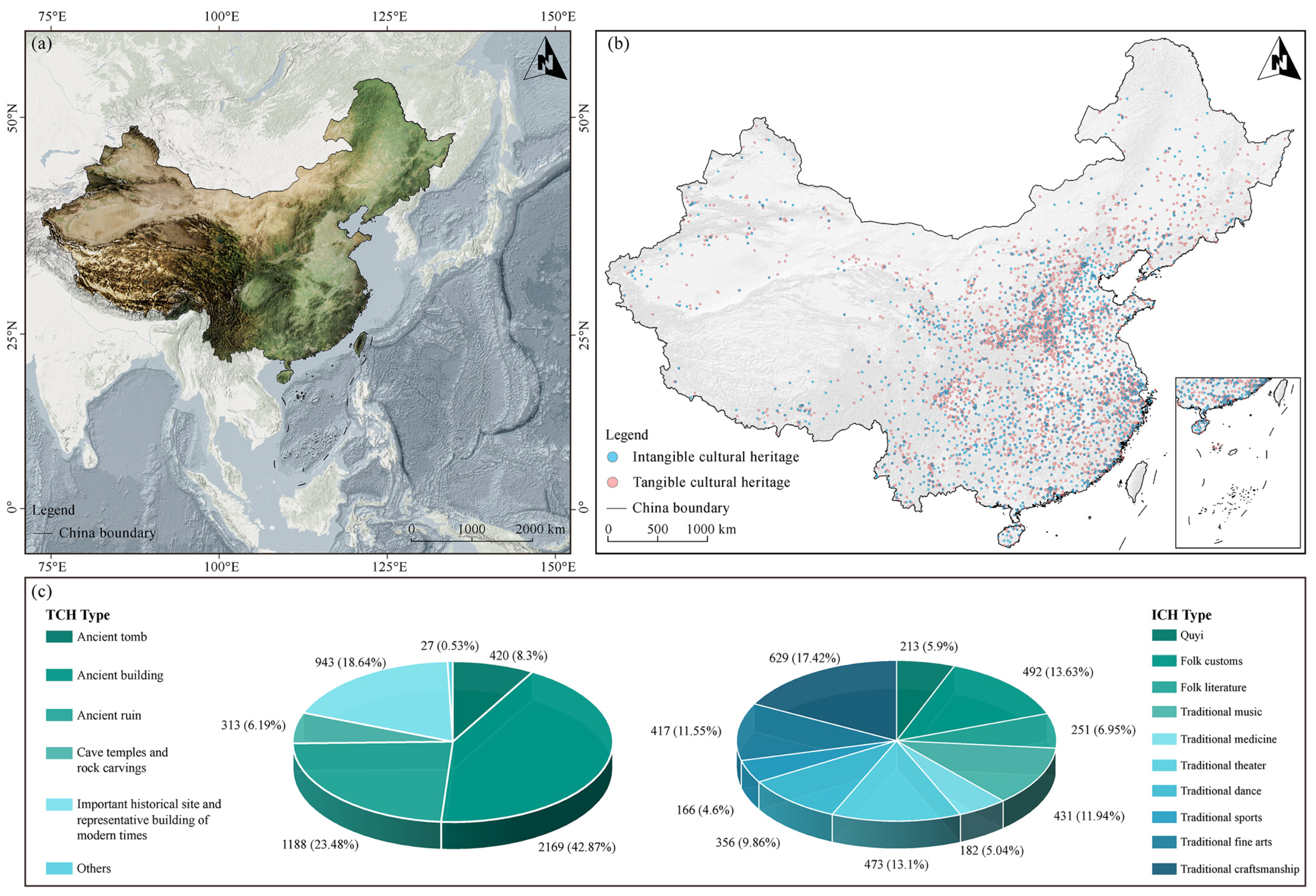
With a history spanning thousands of years, China is located in the eastern part of the Eurasian continent and covers approximately 9.6 million km² (Figure 1). Its three-tiered topographical pattern extending from west to east, combined with complex climatic gradients, has shaped diverse geographical units that constitute a natural arena for cultural differentiation and integration among the country’s 56 ethnic groups [30]. A total of 5060 national-level cultural relic protection units, ranging from the Neolithic period to the present day, form a comprehensive spectrum of TCH, encompassing ancient architecture, archeological sites, and other typological categories. Additionally, 3610 ICH items are distributed across ten categories, including folk literature, traditional music, and customs. The historical information and human–land relations embedded within these two types of heritage reflect the transnational value of Chinese culture in engineering technology, ceremonial institutions, and ideological frameworks. The spatial distribution of this heritage, characterized by distinct geographical differentiation and clustering patterns, reflects the evolutionary logic of cultural patterns [31] and provides crucial empirical samples for global cultural heritage research. China’s cultural heritage protection system represents a significant experiential supplement to the World Heritage Convention, holding substantial practical significance for investigating the coupling characteristics and influencing mechanisms of heritage spatial distribution.

Figure 1. Spatial distribution and TCH/ICH proportions of cultural heritage in China. (a) Geographic location of China; (b) spatial distribution of tangible and intangible cultural heritage sites; (c) proportional distribution of TCH and ICH by category.

2.2. Data Sources

TCH was determined based on a list of national key cultural relics protection units published by the National Cultural Heritage Administration, and their spatial coordinates were obtained using the Baidu coordinate retrieval system. ICH data were derived from the standardized dataset compiled by Guo Y. et al., organized by the geographical location of the applying regions or institutions [32]. Data on the proportion of the tertiary industry, per capita GDP, and the population share of different ethnic groups were obtained from statistics publicly available on government websites. Ethnic diversity was calculated using the Shannon–Wiener index [33], which measures social group richness based on the population share of each ethnic group. Provincial-scale digital elevation model (DEM) data (https://www.resdc.cn/data.aspx?DATAID=337, accessed on 11 March 2025) and geological hazard points (https://www.resdc.cn/data.aspx?DATAID=290, accessed on 10 March 2025) were obtained from the Resource and Environmental Science Data Platform. Elevation, aspect, and slope parameters were then extracted from these using ArcGIS Pro 3.1.4. The 1 km mean annual temperature raster was obtained from the China extreme and average temperature index dataset (1961–2012), provided by the National Tibetan Plateau Data Center [34]. The 1 km mean annual precipitation data were derived from the monthly precipitation dataset developed by Peng S. et al. [35] and converted into the appropriate units after being aggregated to annual values. The 30 m resolution Normalized Difference Vegetation Index (NDVI) raster was obtained from the research outputs of Dong J. et al. [36] and Yang J. et al. [37]. The 100 m population density raster was sourced from the Lake–Watershed Science Data Center, National Earth System Science Data Center, National Science & Technology Infrastructure of China [38] (http://lake.geodata.cn, accessed on 7 March 2025). Road and hydrographic data were obtained from the Geospatial Data Cloud (http://www.gscloud.cn, accessed on 12 March 2025) and OpenStreetMap (https://www.openstreetmap.org/, accessed on 12 March 2025), respectively. All variables corresponding to each geographical unit were processed using spatial statistics in ArcGIS Pro to ensure the spatial consistency of the attribute data, thereby supporting subsequent modeling and analysis.

2.3. Data Processing and Variable Selection

To ensure data quality and model robustness, this study employed a standardized data processing workflow. First, samples with missing coupling degree values were removed. Median imputation was then used to handle missing values in feature variables, thereby minimizing distributional assumptions and reducing sensitivity to outliers [39]. Subsequently, the interquartile range (IQR) method was used to identify and remove outliers [40]. To improve skewed data distributions and enhance model convergence within the Bayesian framework, the Yeo–Johnson transformation was applied to all continuous variables:

$$Y^{(\lambda )}=\left\{\begin{array}{ll}{\displaystyle \frac{{(Y+1)}^{\lambda }-1}{\lambda }},\hfill & \mathrm{if} Y\ge 0,\hspace{0.33em}\lambda \ne 0\hfill \\ \ln (Y+1),\hfill & \mathrm{if} Y\ge 0,\hspace{0.33em}\lambda =0\hfill \\ -{\displaystyle \frac{{(-Y+1)}^{2-\lambda }-1}{2-\lambda }},\hfill & \mathrm{if} Y<0,\hspace{0.33em}\lambda \ne 2\hfill \\ -\ln (-Y+1),\hfill & \mathrm{if} Y<0,\hspace{0.33em}\lambda =2\hfill \end{array}\right.$$

(1)

In Equation (1), Y represents the original data; the transformation parameter, λ, is determined using the maximum likelihood estimation method to correct the transformation shape [41].

To eliminate scale effects and ensure comparability between different features, Z-score standardization was applied to the transformed data [42].

The aforementioned workflow optimized data characteristics while preserving the underlying relational structures required for causal inference methods. In this study, drivers are formally defined as covariates that, after controlling for confounding variables and spatial scale effects, exhibit a directionally clear and statistically significant non-zero effect on the coupling index. This definition aims to link mechanisms such as economic structure and environmental exposure to the TCH–ICH coupling process and to examine their cross-regional heterogeneity. Regarding indicator selection, we conducted correlation analysis, multicollinearity testing, and significance testing on 13 baseline features and their constructed bivariate interaction terms, with the final variable set determined based on posterior inference. The construction of interaction variables was guided by both empirical verification of indicators and consideration of established theories, such as infrastructure complementarity and economic agglomeration effects [43].

To further assess the potential causal relevance and statistical robustness of the variables, the instrumental variables method [44] was employed to validate all potential factors. When an instrumental variable passes the weak instrument test (F-statistic > 10) and the second-stage regression yields p < 0.1, it receives a score of 2. Variables that fail the test but have second-stage regression (p < 0.1) receive a score of 1. Those that are significant only in conventional regression (p < 0.1) but lack valid instrumental variables receive a score of 0.5. This scoring scheme was designed to quantify the strength of causal evidence, rather than make definitive causal claims. Combined with the significance levels obtained from the HBM, the primary treatment variables were designated as those that were significant and had a score of 2. These variables serve as core explanatory variables for causal effects and their heterogeneity. Those that were significant and had a score of 1 were designated robustness variables for sensitivity analysis. Non-significant variables with a score of 0.5 were designated as exploratory variables to capture potential specificities. It should be noted that some variables exhibited relatively weak instrumental strength, indicating uncertainty in the causal effect estimates. Therefore, a dual-validation strategy was adopted to enhance the robustness of the results.

Theoretically, factors such as climate and topography are linked to heritage through their influence on population distribution. To statistically isolate these baseline effects, an analytical framework was constructed to support causal inference. Its primary task was to control for confounding factors in order to estimate the net effects of key variables on heritage coupling, thereby addressing the scientific question of why and how such coupling occurs. Thus, by disentangling complex interdependencies, this approach mitigated the risk of tautological reasoning regarding human–heritage correlations and helped to reveal the differentiated mechanisms driving the spatial coupling of heritage.

2.4. Research Methods

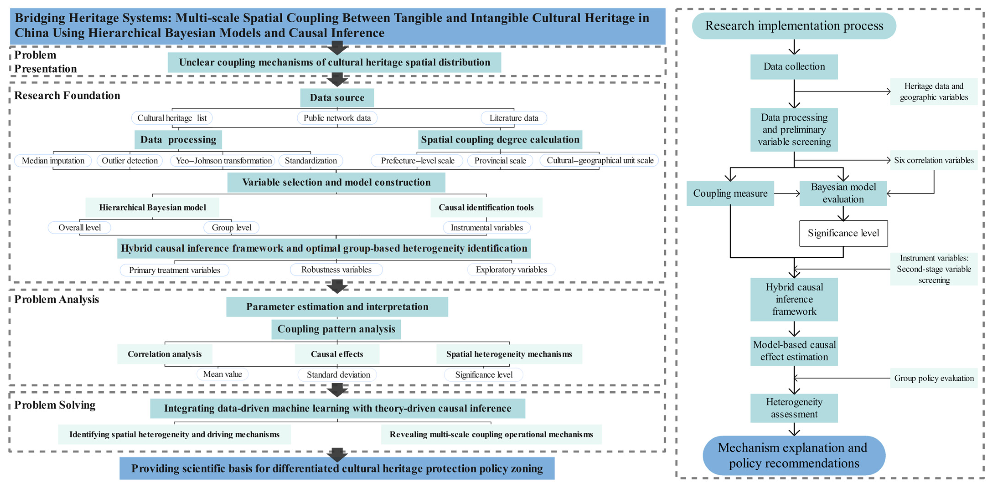
We developed a progressive analytical framework integrating multi-scale identification, hierarchical modeling, and causal validation. First, the degree of heritage coupling was measured based on the processed data, and correlations for the initially screened variables were identified using a Bayesian model. Subsequently, three types of variables were re-screened based on significance levels and instrumental variables, enabling the identification of model-based causal effect estimates and heterogeneity under optimal grouping strategies (Figure 2).

Figure 2. Research framework and implementation workflow diagram. Dark blue (R126, G175, B220): research title and significance; teal (R177, G219, B223): core analytical frameworks and processes; light green (R233, G248, B245): methods and supporting information.

(1)

Spatial Coupling Degree Calculation Method

Coupling describes the dynamic relational mechanisms through which system components interact and co-evolve, and it has been assigned multiple meanings across disciplines, including correlation and interdependence. The term ‘coupling’ is used in heritage studies to refer to the cultural and social associations reflected through spatial co-location. Due to potential shared historical trajectories, social transformations and environmental constraints, spatial co-location constitutes a core condition for heritage coupling [9]. For example, traditional villages and historic buildings often form cultural ensembles together with folk customs, festivals and ritual practices [16]. Such symbiotic relationships between TCH and ICH represent a marker of cultural system integrity and have given rise to holistic conservation approaches that emphasize their interconnections [45].

Drawing on system coupling theory [46] and research on place attachment in cultural geography [47], this study integrated spatial analysis with cultural interpretation. The term ‘coupling’ refers to the association strength at the level of spatial co-location, measured through operational indicators, that is, the systematic co-existence patterns in which TCH and ICH deviate from a random spatial distribution. Spatial coupling analysis does not equate ‘coupling’ with mere ‘proximity’, but instead conceptualizes spatial co-location as a spatial representation of cultural associations [48]. A high degree of coupling indicates that the two have formed a closely interconnected cultural ecosystem whose spatial clustering patterns reflect functional complementarity and cultural symbiosis. This theoretical lens shifts the meaning of heritage from isolated elements to the relational networks formed among them [49]. Accordingly, the measurable mathematical indicator captures statistical proximity and spatial evidence of interactive relationships between TCH and ICH.

This study used the modified co-location quotient (MCLQ) index to quantify the coupling intensity between TCH and ICH. Based on the CLQ theoretical framework, this method assesses the degree of association of point features by comparing the actual number of neighboring point pairs observed with the expected value under theoretical random distribution conditions [50]. The CLQ method is often adapted in spatial co-location analysis to suit the characteristics of different datasets [51]. A correction coefficient was introduced to adjust for the impact of geographical unit boundaries on the effective search area of heritage sites. Additionally, a geographical unit-based analytical framework was adopted, with differentiated search radii designed accordingly.

The number of neighboring point pairs satisfying the distance threshold conditions was first calculated:

$$C_i={\displaystyle \sum _{j=1}^m{\displaystyle \sum _{k=1}^{n}I}}(D_{jk}\le r)$$

(2)

Here, m and n denote the number of TCH and ICH points within a geographic unit, respectively; D_jk represents the Euclidean distance between TCH point j and ICH point k; and I(⋅) is an indicator function that takes the value 1 when the distance condition is satisfied, and 0 otherwise.

The expected number of nearest-neighbor point pairs was estimated under the assumption that heritage points were randomly distributed within the unit, determined by the ratio of the search area to the unit area. A correction factor was applied to account for the reduction in the effective search area for heritage points located near the unit boundaries.

$$E_i={\displaystyle \frac{m\times n\times \pi r^2}{A_i}}\times \lambda$$

(3)

$$\lambda =\min \left(1,{\displaystyle \frac{A_i}{\pi r^2}}\right)$$

(4)

In the above equations, A_i represents the area of the geographical unit (km²); λ represents the boundary effect correction coefficient; and r represents the search radius.

Finally, standardized MCLQ values were obtained by comparison with the values expected under a random distribution.

$${\mathrm{MCLQ}}_i={\displaystyle \frac{C_i}{E_i}}$$

(5)

Geographical units were classified into four coupling types based on MCLQ values: strongly coupled areas (MCLQ > 2.0), characterized by high spatial clustering and strong co-distribution of both heritage types; weakly coupled areas (1.0 < MCLQ ≤ 2.0), exhibiting moderate spatial association; independently distributed areas (0.5 ≤ MCLQ ≤ 1.0), exhibiting relatively random distribution patterns; and repulsively distributed areas (MCLQ < 0.5), exhibiting spatial separation between the two heritage types.

Considering China’s administrative system and geographical characteristics, the analysis units were defined at three geographical scales: prefecture-level scale, provincial scale, and cultural–geographical unit scale. The search radii were set at 20 km, 150 km, and 250 km, respectively. This multi-scale framework follows place formation theory [52], recognizing that heritage associations are products of multi-level social processes [53]. Smaller radii are suited for identifying community-level symbiotic relationships, while larger radii can capture association patterns within cultural networks. Different radii correspond to different natural or social scales, reflecting interactive processes at various levels [54]. Historically, cultural practices within prefecture-level administrative units or settlements primarily unfolded within daily life circles and transportation networks [55]. Based on this theory, the 20 km radius was set to correspond to local interaction ranges, capturing the functional symbiotic relationships between TCH and ICH. Provincial administrative divisions often follow natural geographical boundaries and have important cultural and institutional integration functions. The 150 km radius was set to correspond to the spatial scale of regional cultural networks, capturing co-distribution patterns [56]. China’s cultural geography is divided into seven regions. These units share common historical origins and cultural concepts, forming cultural ecological zones that transcend administrative boundaries [57]. The 250 km radius was set to capture spatial evidence of cultural diffusion and heritage evolution at the macro scale, identifying coupling patterns driven by geo-historical processes. This differentiated configuration considered the average spatial extent of geographical units and the distribution density of heritage sites at each scale, ensuring the effective identification of cross-scale spatial associations [58].

From the perspective of conservation practice, a strong coupling state signals active functional linkages, whereas a weak coupling state may indicate breaks in cultural transmission. This observation is consistent with the phenomena of cultural continuity and functional discontinuity documented in studies of traditional villages [57]. The coupling types described above are regarded as external manifestations of latent cultural interactions, but they do not directly reveal underlying social or cultural relations. Relying solely on this diagnostic indicator cannot quantify the social or environmental driving mechanisms, so we constructed interaction terms and implemented machine-learning models. This approach enabled us to empirically test the actual effects of factors and mechanism pathways, link spatial attributes to cultural or social explanatory mechanisms, and thereby strengthen the scientific validity of the coupling-system indicators.

(2)

Hierarchical Bayesian Model

The core of HBM lies in nesting effects at both the overall level and group level, achieving information sharing and bias correction through hyperparameter constraints [59]. Compared with traditional regression methods, HBM not only avoids underestimation of standard errors caused by ignoring intra-group correlations but also maintains robustness under conditions of unbalanced sample sizes across groups or sparse local data [60]. This characteristic effectively integrates the regional heterogeneity and multi-level data structures of the three types of geographical units, thereby preventing the information loss that would result from single-level models.

The three geographical grouping patterns were used as grouping criteria, enabling separate modeling at each geographical level and revealing the similarities and differences between the overall and local effects [61]. The sample was randomly divided, with 80% allocated to the training set and the remainder to the test set, thus balancing the requirements for model training and independent validation. The basic model form is as follows:

Group level: Data from each group are directly processed for fitting, and the Markov Chain Monte Carlo (MCMC) method is used to estimate parameters for each group [62]. This method preserves inter-group differences through independent sampling. Group-specific parameters are subject to structural constraints due to shrinkage effects, which prevent overfitting by exhibiting a tendency to shrink toward the overall mean [63].

$$y_{ij}~\mathcal{N}({\mu }_{ij},{\sigma }^2),\hspace{1em}{\mu }_{ij}={\alpha }_j+{\displaystyle \sum _{k=1}^K{\beta }_{jk}}{X}_{ijk}$$

(6)

In Equation (6), y_ij represents the MCLQ value of the i-th observation in the j-th group; X_ijk represents the k-th feature variable; β_jk is the corresponding regression coefficient, revealing the variable effects within different groups; α_j represents the group-specific intercept term; and σ² represents the variance parameter.

Overall level: Imposing weakly informative hyperpriors on group-level intercepts and slopes stabilizes estimates for small-sample groups while preserving between-group heterogeneity. When sample sizes are small or residual variance is large, posterior estimates become more sensitive to hyperpriors [64]. Tighter variance hyperpriors strengthen partial pooling, draw small-sample parameters toward the overall mean, and suppress extreme estimates, thereby reducing overfitting. Looser variance hyperpriors widen uncertainty and more fully reveal cross-group differences. The mean hyperprior determines the direction and magnitude of shrinkage. Accordingly, a zero-centered, weakly informative specification with an appropriate scale helps avoid systematic bias in small-sample groups [65]. The hyperprior on the residual term also indirectly modulates shrinkage in small groups by altering the effective noise level.

$${\alpha }_j~\mathcal{N}({\mu }_{\alpha },{\tau }_{\alpha }^2),\hspace{1em}{\beta }_{jk}~\mathcal{N}({\mu }_{{\beta }_k},{\tau }_{{\beta }_k}^2)$$

(7)

Here, μ_α and μ_βk serve as hyperpriors representing overall-level mean effects; ${\tau }_{\alpha }^2$ and ${\tau }_{\beta k}^2$ are variance parameters reflecting the degree of effect variation across different geographical units.

The model captures overall patterns and inter-group variations through a multi-layered parameter structure, enabling cross-scale effect decomposition. Uncertainty quantification provides complete posterior probability distributions for the estimated parameters. MCMC sampling convergence was diagnosed using the Gelman–Rubin statistic (Rˆ) and Monte Carlo standard error (MCSE) [66]. For model evaluation, the coefficient of determination (R²) was employed to quantify the model’s fitting capability [67]. Root mean square error (RMSE) was used to measure the accuracy of the model’s predictions [68]. The Bayesian p-value (BPV) was introduced to test the consistency between the observed and generated data [69]. Together, these three metrics provided comprehensive evaluation criteria for HBM performance from the perspectives of goodness of fit, prediction accuracy, and statistical validity. In addition, five-fold cross-validation was used to assess out-of-sample predictive stability. One of the five randomly partitioned subsets was designated as the test set and the remaining subsets as the training set, with fitting and prediction repeated across folds. The RMSE and mean absolute error (MAE) on each test fold were then averaged to quantify generalization performance [70].

To further assess whether the hierarchical structure of the HBM had adequately captured spatial dependence, multi-strategy spatial autocorrelation diagnostics were applied to the model residuals. Given the sensitivity to the specification of spatial weight matrices, three robustness schemes [71] were implemented: (a) queen contiguity matrices; (b) adaptive distance–band matrices with thresholds set at the 75th and 90th percentiles of the k-nearest-neighbor (KNN) distance distribution (with k = 8, 6, and 3 for the three geographical scales); and (c) KNN matrices chosen to balance statistical power in small samples against over-connection in large samples (with k = 6, 3, and 2 for the three scales). All weight matrices were row-standardized to ensure comparability across heterogeneous neighborhood structures [72]. For each specification, the global Moran’s I of the residuals was computed, and significance was assessed using a 999-permutation Monte Carlo test [71]. If the residuals exhibited no significant spatial autocorrelation across all strategies (p > 0.05), we concluded that the HBM had sufficiently captured spatial dependence, obviating the need for additional spatially structured terms.

(3)

Causal Effect Estimation and Heterogeneity Analysis

A hybrid causal inference framework based on double machine learning (DML) and ordinary least squares (OLS) was employed to investigate the causal mechanisms underlying the cultural heritage coupling. Within this framework, the DML approach was used to control for high-dimensional confounders and reduce model specification bias [73], while the OLS approach was used to retain interpretability. This design ensured accurate estimation and robust, reliable identification of causal effects. The basic mathematical structure is expressed as follows:

$$Y_i=\alpha +\beta T_i+\gamma X_i+{ϵ}_i$$

(8)

$$Y_i=\theta T_i+g(X_i)+{ϵ}_i$$

(9)

$$T_i=m(X_i)+{\nu }_i$$

(10)

$$\widehat{g}(x)={\rm E}[Y| X=x],\hspace{1em}\widehat{m}(x)={\rm E}[T| X=x]$$

(11)

$${\widehat{\theta }}_{\mathit{DML}}={\left({\displaystyle \sum _{i=1}^n{(T_i-\widehat{m}(X_i))}^2}\right)}^{-1}{\displaystyle \sum _{i=1}^n(T_i-\widehat{m}(X_i))}(Y_i-\widehat{g}(X_i))$$

(12)

Equation (8) specifies the OLS regression model used as the baseline estimation. Y_i denotes the MCLQ value of the i-th geographical unit; T_i represents the treatment variable; X_i is the vector of the control variables; β is the target causal effect parameter; γ is the coefficient vector for the control variables; α is the intercept term; and ϵ_i is the random error term.

Equations (9)–(12) present the core structure of the DML method [74]. θ denotes the target causal effect parameter (average treatment effect, ATE); $\widehat{g}(X_i)$ and $\widehat{m}(X_i)$ denote the estimated conditional expectation functions of the outcome and treatment variables with respect to the covariates; ϵ_i and ν_i are the random error terms; ${\widehat{\theta }}_{\mathit{DML}}$ is the causal effect estimated by DML; $(T_i-\widehat{m}(X_i))$ is the residualized treatment variable that removes the influence of control variables; $(Y_i-\widehat{g}(X_i))$ is the residualized outcome variable that eliminates the effect of control variables; and n is the sample size.

The DML estimation required randomly splitting the sample into K folds to implement a cross-fitting strategy [75]. Using data from the other folds, $\widehat{g}(X_i)$ and $\widehat{m}(X_i)$ were estimated separately based on the random forest algorithm and then used to predict the target fold. The number of trees was adaptively adjusted according to the sample size to balance estimation accuracy and overfitting risk. The maximum tree depth was constrained using a logarithmic function based on the sample size, and a feature subsampling strategy was employed to reduce variance. Residuals were then computed to ensure the unbiasedness of the causal effect estimates. Finally, ordinary least squares regression was performed on the residualized variables, and the causal effect estimates from each fold were weighted by sample size to obtain ${\widehat{\theta }}_{\mathit{DML}}$.

We employed Conley heteroscedasticity and autocorrelation consistent (HAC) standard errors to assess the robustness of our causal estimates to potential spatial autocorrelation [76]. Given the asymptotic nature of Conley–HAC and the small sample sizes at the other two scales, the main analysis was conducted only for the prefecture-level sample. Bandwidths were chosen in a data-driven manner: we used the 25th and 50th percentiles of the nearest-neighbor distances between city centroids as the lower and main bandwidths and determined an adaptive bandwidth by requiring that ≥70% of nodes had at least one neighbor. Distances were computed as projected Euclidean distances, and spatial weights were constructed using the Bartlett (triangular) kernel [77]. Variable selection focused on pre-specified main treatment variables and robustness-check variables to mitigate post-selection inference bias.

For the best grouping identified through subsequent multi-group strategies, the significance and degree of heterogeneity were assessed using Cochran’s Q test and the I² statistic, respectively [78]. The Q statistic follows a chi-square distribution with k − 1 degrees of freedom. Typically, I² > 75% indicates high heterogeneity, 25% < I² ≤ 75% indicates moderate heterogeneity, and I² ≤ 25% indicates low heterogeneity.

To ensure reliable causal inference, differentiated robustness checks were constructed based on the theoretical importance of variables and the strength of causal evidence [79].

$${\Delta }_{\mathrm{robust}}={\displaystyle \frac{|{\widehat{\theta }}_{\mathrm{extended}}-{\widehat{\theta }}_{\mathrm{base}}|}{\left|{\widehat{\theta }}_{\mathrm{base}}\right|}}\times 100\%$$

(13)

$${\Delta }_{\mathrm{norm}}={\displaystyle \frac{|{\widehat{\theta }}_{\mathrm{OLS}}-{\widehat{\theta }}_{\mathrm{DML}}|}{\sqrt{\left({\mathrm{SE}}_{\mathrm{OLS}}^2+{\mathrm{SE}}_{\mathrm{DML}}^2\right)}}}$$

(14)

Equation (13) tests for the influence of potential confounding variables on the main effect. If the change in effect is less than 20%, the results are considered robust. ${\widehat{\theta }}_{\mathrm{base}}$ and ${\widehat{\theta }}_{\mathrm{extended}}$ denote the estimated causal effects of the main treatment variable in the baseline model and the extended model that incorporates robustness variables, respectively. Equation (14) compares the estimation differences between the two methods. If Δ_norm < 1.96, the results are considered statistically consistent across the two methods. SE_OLS and SE_DML represent the standard errors of the two estimates, respectively.

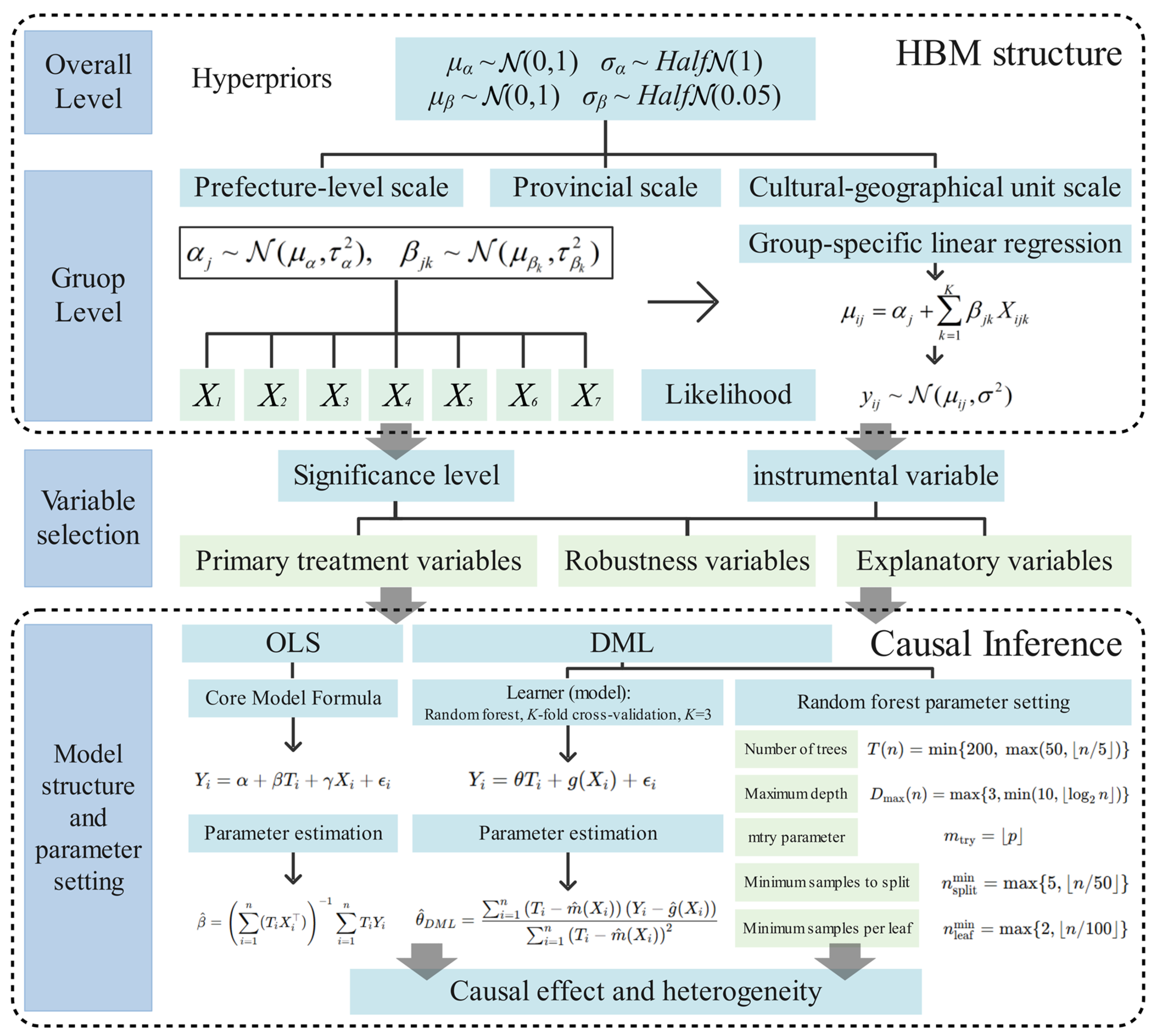
A rigorous, comprehensive test was conducted for the primary treatment variables. Potential confounding variables were added sequentially to examine the stability of their coefficients, and the consistency of the method was verified across the baseline and each extended model. For robustness variables, the focus was on assessing methodological consistency, supplemented by a simplified version of Equation (13) to test the effects of key control variables and avoid excessive testing. For exploratory variables, the emphasis was placed on evaluating the stability of the coefficients across different model specifications. Consistency checks between methods were only performed for significant variables in the baseline model. Furthermore, to clearly illustrate the complex structure of the constructed HBM and causal inference models, Figure 3 displays the hierarchical structure, prior distribution specifications, and core parameters.

Figure 3. Schematic diagram of the HBM and causal inference model structure.

If longitudinal data become available, the framework can be extended temporally. The HBM can be extended to a cross-classified spatiotemporal hierarchy, where time-varying random intercepts and key slopes with weak temporal-dependence priors are introduced within each geographic scale. Spatially structured components can also be combined with the temporal process through a separable space–time covariance [80], preserving cross-scale analysis while providing spatiotemporal trajectories of key driver effects. Concurrently, the causal module can be extended via a two-way fixed-effects difference-in-differences design [81]. By aligning units to the onset of treatment and incorporating lead and lag indicators, dynamic effect paths can be estimated in an event-study form, using cluster-robust standard errors to ensure robustness against serial correlation [82].

(4)

Optimal Grouping Strategy for Heterogeneity Analysis

We used a multidimensional evaluation framework to identify the optimal grouping strategy for heterogeneity. Sample units were grouped according to key variables, enabling causal effects to be analyzed comparatively within each group. Four grouping methods were applied: median split, tertile split, quartile extreme, and K-means clustering. The composite scoring function encompassed three aspects: statistical significance testing, effect size measurement, and the magnitude of intergroup differences.

To quantify the differences between the groups, Cohen’s d and Partial Eta Squared were used as effect size indices for two-group and multiple-group comparisons, respectively [83]. The corresponding calculation formulas are as follows:

$$d={\displaystyle \frac{{\overline{X}}_1-{\overline{X}}_2}{s_{\mathrm{pooled}}}}$$

(15)

$$s_{\mathrm{pooled}}=\sqrt{{\displaystyle \frac{(n_1-1)s_1^2+(n_2-1)s_2^2}{n_1+n_2-2}}}$$

(16)

$${\mathrm{CV}}_{\mathrm{between}}={\displaystyle \frac{\sigma ({\overline{X}}_1,{\overline{X}}_2,\dots ,{\overline{X}}_k)}{\overline{X}}}$$

(17)

Cohen’s d effect size is typically classified as small (d ≈ 0.2), medium (d ≈ 0.5), or large (d ≈ 0.8). The coefficient of variation between groups (CV_between) measures the relative dispersion among group means, with values greater than 0.4 indicating a large effect size.

Based on these parameters, the magnitude of intergroup differences was introduced to evaluate the performance disparities across different classification combinations. The optimal combination was required to reach statistical significance (p < 0.05) and to exhibit a large effect size [84]. Additionally, each group had to meet the sample size requirement for statistical inference (n ≥ 30), and the grouping results had to be consistent with geographical and social logic. This weighting scheme emphasized the central role of effect size while assigning equal importance to statistical significance and the magnitude of group differences.

$$\mathrm{Score}=0.2\times (1-p)+0.6\times \mathrm{Effect} \mathrm{Size}+0.2\times {\displaystyle \frac{\Delta \mu }{\max (\Delta \mu )}}$$

(18)

where p represents the significance level obtained from statistical testing; Effect Size represents the standardized effect size; Δμ represents the mean difference between groups; and max(Δμ) represents the maximum mean difference.

3. Results

3.1. Multi-Scale Spatial Coupling Patterns of Cultural Heritage

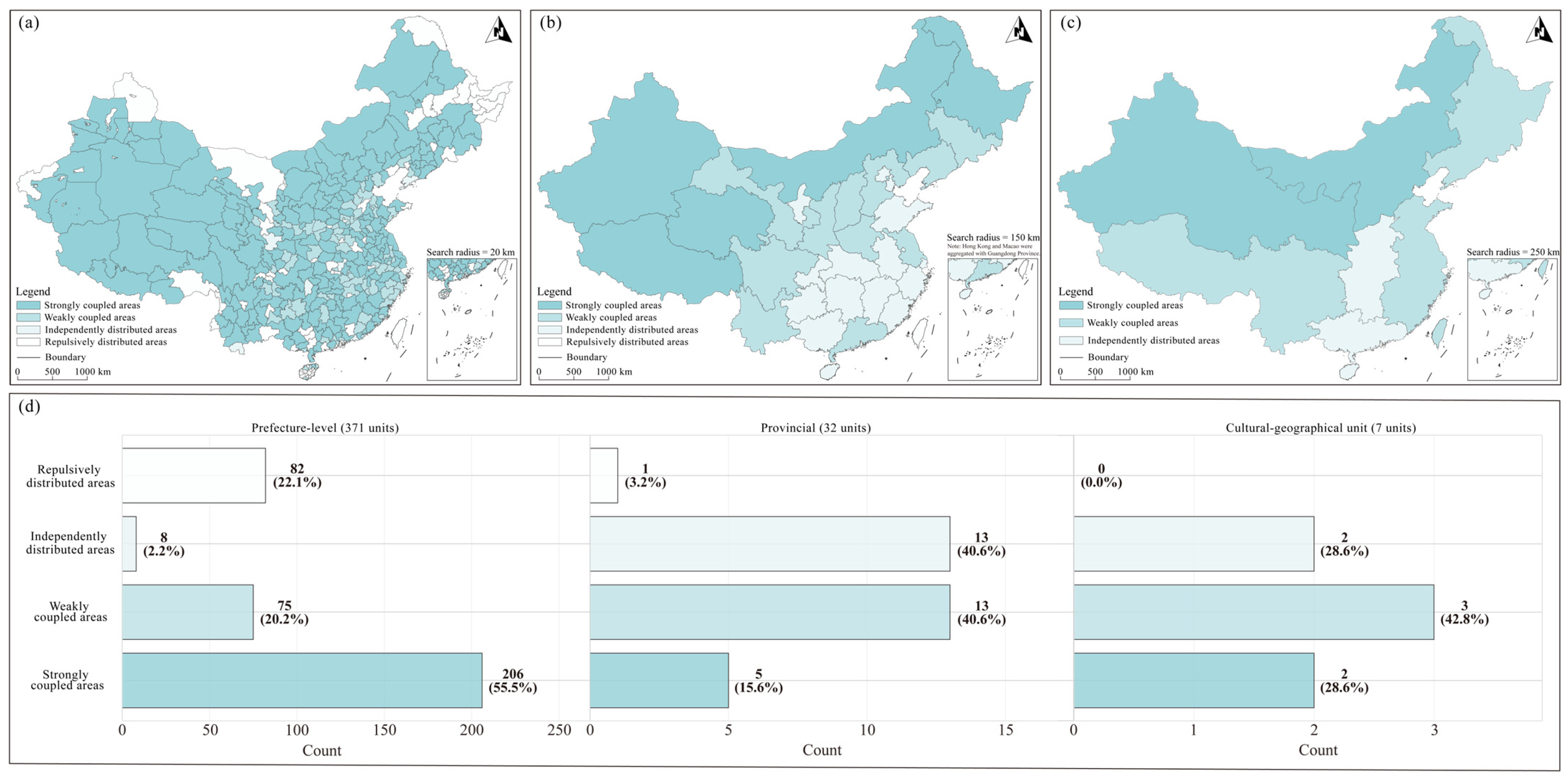
According to the MCLQ index results, the spatial coupling of cultural heritage had a pronounced scale effect across the three analyzed scales (Figure 4). At the prefecture-level scale, strongly coupled areas dominated, accounting for 55.5% of the total, indicating a high degree of co-existence and spatial overlap between the two types of heritage at a fine spatial scale. At the provincial scale, both weakly coupled and independently distributed areas reached their peak proportions of 40.6%, reflecting a weakening and differentiation of heritage associations at intermediate scales. At the cultural–geographical unit scale, the proportions of weakly and strongly coupled areas increased to 42.8% and 28.6%, respectively. These results revealed a reorganization pattern at larger scales, indicating a deviation from the overall trend of continuous weakening in the coupling relationships.

Figure 4. Spatial coupling patterns between TCH and ICH based on MCLQ analysis across three scales. (a) Prefecture-level scale; (b) provincial scale; (c) cultural–geographical unit scale; (d) number of units by coupling type across three scales.

It should be emphasized that the spatial coupling of cultural heritage did not decline monotonically with increasing scale. From the prefecture-level to provincial scale, the proportion of strongly coupled areas decreased markedly while the proportions of weakly coupled and independently distributed areas increased substantially, in line with the general pattern of spatial attenuation. Theoretically, expanding the search range at larger scales would substantially increase the expected value, leading to lower MCLQ indices. However, the proportion of strongly coupled areas rebounded at the cultural–geographical unit scale. This manifested spatially in specific regions in the northwest, north, and northeast, which consistently maintained high coupling—an unexpected response pattern. The re-aggregation trend beyond administrative boundaries at the geographical level may reflect intrinsic cross-regional cohesion and cultural identity [85]. This cross-scale stability suggests that the Chinese cultural system possesses a binding force that maintains connections between TCH and ICH at the macro-spatial level. Consequently, the resulting integrated cultural ecosystem endows the two types of heritage with sufficiently strong associations to overcome the dilution effect at larger scales.

Overall, the prefecture-level scale better reveals local symbiosis between heritage types, while the provincial scale highlights spatial differentiation and independence. The cultural–geographical unit scale reflects the integration and continuity of cultural traditions over a broader area. This comparison underscores the scale sensitivity and regional variability of heritage coupling, the driving mechanisms of which require further quantitative investigation.

3.2. Performance and Diagnostic Assessment of HBM

The three basic variables selected through the aforementioned mechanism were as follows: mean annual temperature (X₁), reflecting regional thermal conditions; the Shannon–Wiener index (X₂), capturing the diversity of ethnic composition; and population density (X₃), representing the density of cultural carriers and the social foundation for heritage transmission. The four interaction variables were as follows: GDP–population interaction (X₄), constructed from per capita GDP and population density, capturing the combined effects of economic development and population size; transport–hydrological network interaction (X₅), comprising road network density and hydrological connectivity, reflecting the synergistic influence of transportation accessibility and water network connectivity; industrial structure (X₆), defined as the interaction between GDP and the proportion of tertiary industry, representing the effect of tertiary sector upgrading on heritage; and topographic–climate interaction (X₇), integrating elevation and mean annual temperature to account for the interplay between topography and climate.

Quantitative validation showed that the selected features had a mean correlation of |r| = 0.309, which was significantly higher than that of the unselected features (|r| = 0.227). Compared with the full-variable model (R² = 0.633), this seven-variable system achieved good explanatory power within a linear approximation framework (R² = 0.612). Additionally, the mean variance inflation factor (VIF) of the selected variables decreased to 1.71, facilitating the maintenance of independence among hierarchical effects and stabilizing parameter estimation in the HBM. Overall, this feature selection strategy achieved an optimized balance between statistical performance and model stability.

The HBM demonstrated strong predictive performance and model fit (Table 1). The R² values for the training and test sets were 0.612 and 0.553, respectively, indicating that the selected covariates and their interaction terms explained 61.2% and 55.3% of the variance in coupling degree, respectively. The RMSE values were 0.456 and 0.504, respectively, demonstrating good predictive accuracy and generalization capability. Cross-validation yielded a mean RMSE of 0.472 ± 0.038 and a mean MAE of 0.294 ± 0.039. The close agreement between the cross-validated RMSE and the test-set RMSE corroborated the reliability of the model evaluation. Moreover, the small standard deviations indicated low sensitivity to the particular data partitioning. The BPV, close to the ideal value of 0.5, suggested adequate model fit without evidence of systematic bias or misspecification. The slight reduction in explanatory power and the controlled increase in prediction error on the test set were both within acceptable thresholds.

Table 1. HBM evaluation metrics.

Evaluation Metrics	Training Dataset	Testing Dataset	Cross-Validation (Mean ± SD)
R2	0.612	0.553	—
RMSE	0.456	0.504	0.472 ± 0.038
MAE	—	—	0.294 ± 0.039
BPV	0.513	—	—

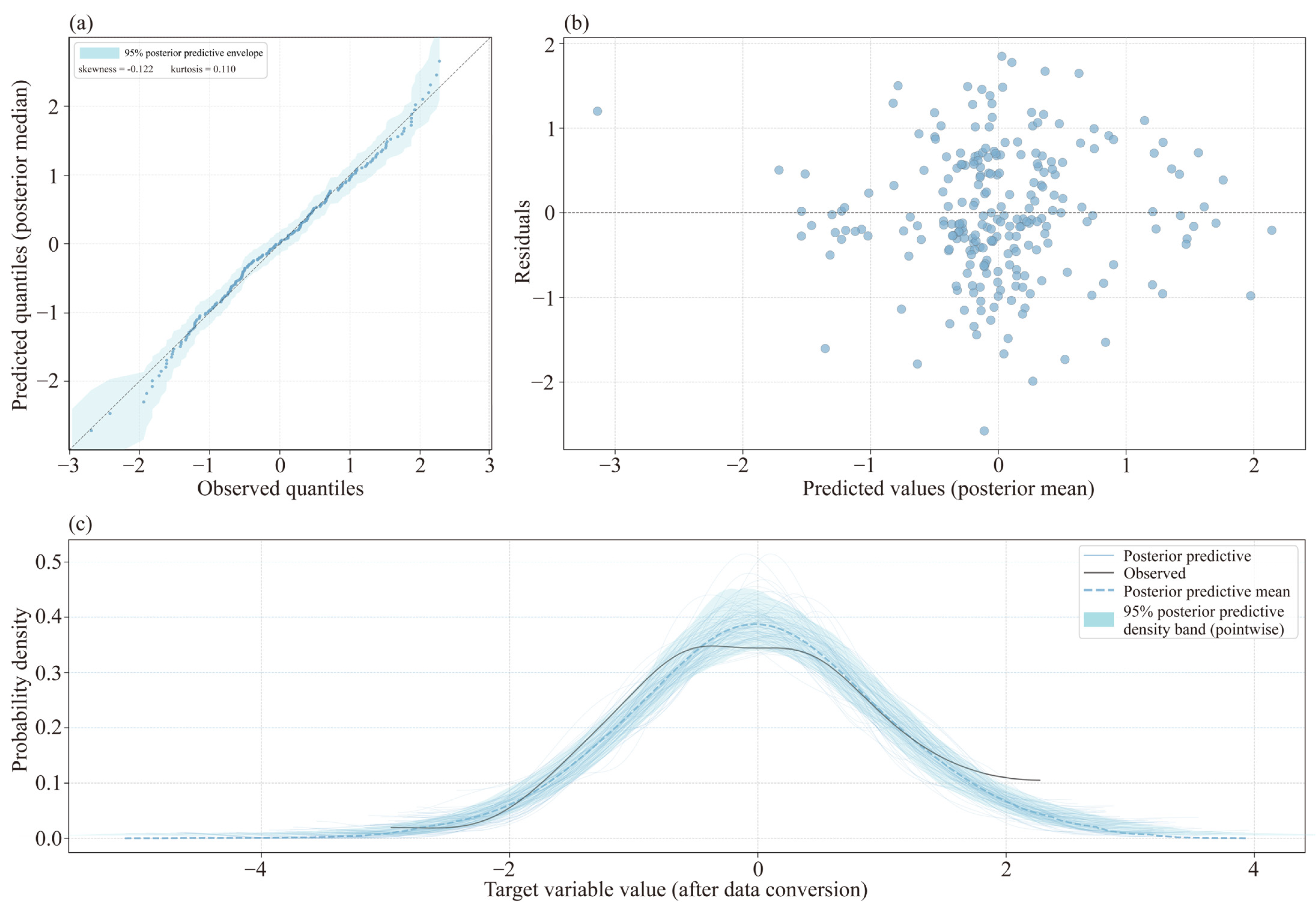
To further assess the fitting quality and the validity of assumptions in the HBM, this study conducted multiple diagnostics based on residual characteristics and predictive performance (Figure 5).

Figure 5. HBM performance diagnostics. (a) Posterior predictive QQ plot; (b) residuals and predicted values; (c) posterior predictive check.

As Figure 5a shows, the data points are closely aligned with the theoretical quantile lines, and the residuals largely conform to the normality assumption. The skewness of −0.122 and the kurtosis of 0.110 are both close to the theoretical value of 0. Only slight deviations occur in the distribution tails, with no evident heavy-tailed or peaked behavior, indicating an absence of significant non-normality [86]. Figure 5b shows no obvious funnel-shaped or systematic patterns, and the residuals exhibit homoscedastic characteristics. The residuals remain relatively uniformly dispersed across the full range, confirming that the model maintains stable predictive accuracy for geographical units at different coupling levels. In Figure 5c, the posterior predictive means largely overlap with the observed data in most regions. The 100 posterior sample curves, reflecting quantified uncertainty, display approximately unimodal normal distributions similar to the observed data. The peak positions largely coincide, and the distribution widths and tail decay patterns are comparable, indicating that the model successfully captures the underlying probabilistic generative process of the coupling degree.

Multi-strategy spatial autocorrelation diagnostics indicated that the HBM residuals showed no significant spatial dependence at any scale (Table 2), suggesting that the hierarchical structure had appropriately modeled spatial association. At the prefecture-level scale, Moran’s I ranged from 0.0029 to 0.0391 (p = 0.06–0.45). At the provincial scale, residual spatial structuring was even weaker, with Moran’s I between −0.0692 and 0.0017 (p = 0.36–0.47). Despite the very small sample size at the cultural–geographical unit scale, the results remained non-significant (p = 0.25–0.49). All diagnostic strategies supported residual spatial independence. Accordingly, no additional spatially structured terms were introduced, thereby avoiding the risk of over-parameterization.

Table 2. Residual spatial autocorrelation diagnostics for the HBM across scales.

Geographic Scale	Weight Matrix	Moran’s I	z-Score	p-Value
Prefecture-level	Queen contiguity	0.0029	0.15	0.45
	Distance band (309.7 km)	0.0391	1.38	0.08
	Distance band (393.3 km)	0.0364	1.59	0.06
	KNN (k = 6)	0.0273	0.94	0.17
Provincial	Queen contiguity	−0.0692	−0.21	0.42
	Distance band (1011.4 km)	−0.0381	0.02	0.47
	Distance band (1307.6 km)	−0.0581	−0.25	0.43
	KNN (k = 3)	0.0017	0.31	0.36
Cultural–geographical unit	Queen contiguity	−0.0499	0.53	0.25
	KNN (k = 2)	−0.1838	−0.07	0.49

Overall, the HBM achieved stable predictive accuracy and residual spatial independence across scales, supporting its use as a reliable basis for subsequent causal inference without additional spatial terms.

3.3. Posterior Inference Results of HBM

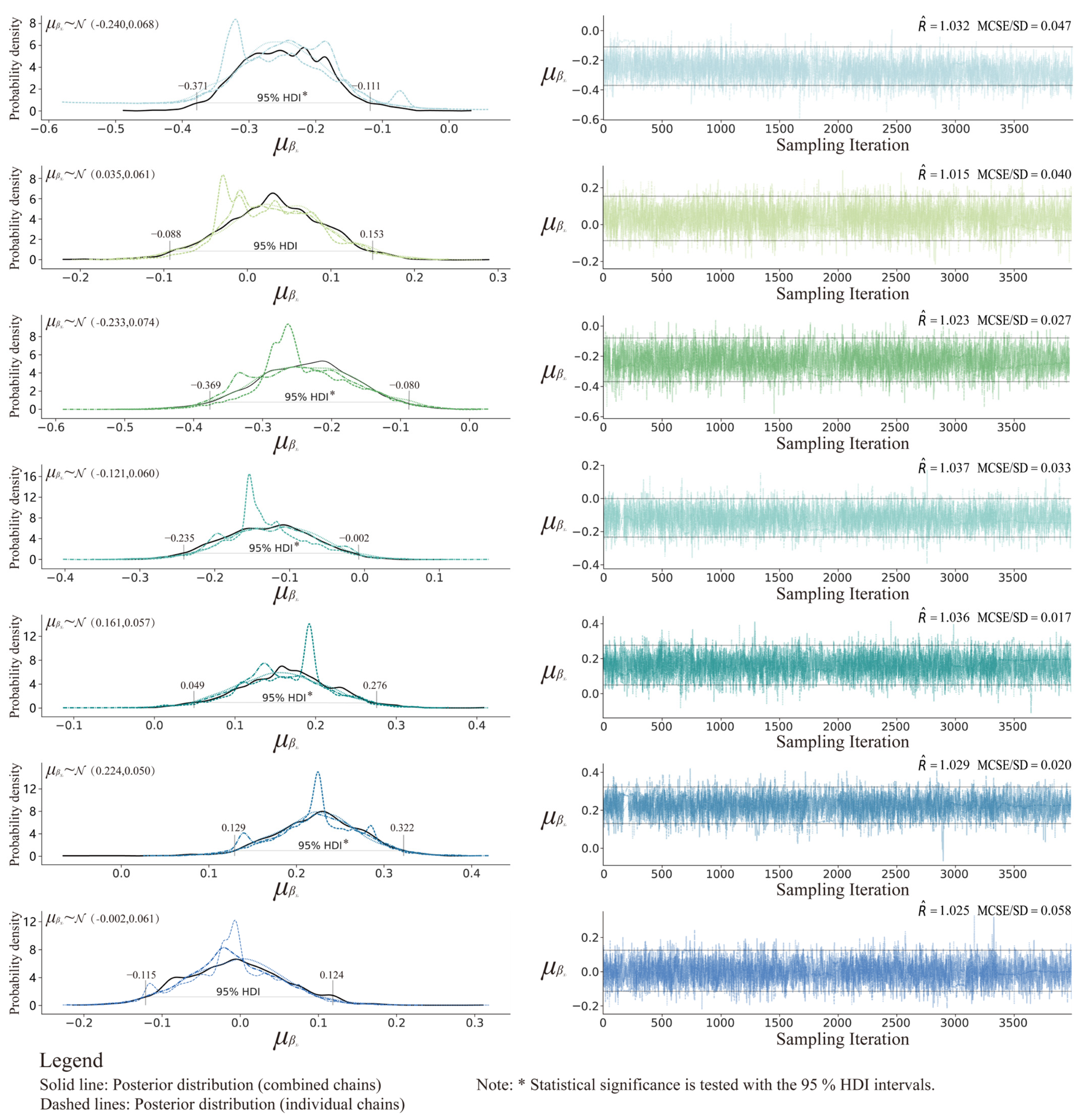
Based on the diagnostics of the MCMC chains, the sampling trajectories of the β parameters at the overall level exhibit good mixing (Figure 6). The trajectories display stable random-walk patterns within the target range, with no apparent drift or stagnation, indicating that the model converged to a stable posterior distribution. Convergence diagnostics show that the $\widehat{R}$ values are all below the convergence threshold of 1.1 and fall within the [1.015, 1.037] range. As a proportion of the posterior standard deviation, the MCSE is below 5% for all parameters, generally satisfying the required sampling precision. The dashed lines on the left indicate that the posterior distributions of the three scale groups differ significantly, confirming that the HBM successfully captures the statistical characteristics of between-group differences.

Figure 6. Posterior distributions and MCMC samples of overall level regression coefficients. Colors indicate individual variables, with each variable’s posterior distribution and corresponding MCMC samples shown in the same color.

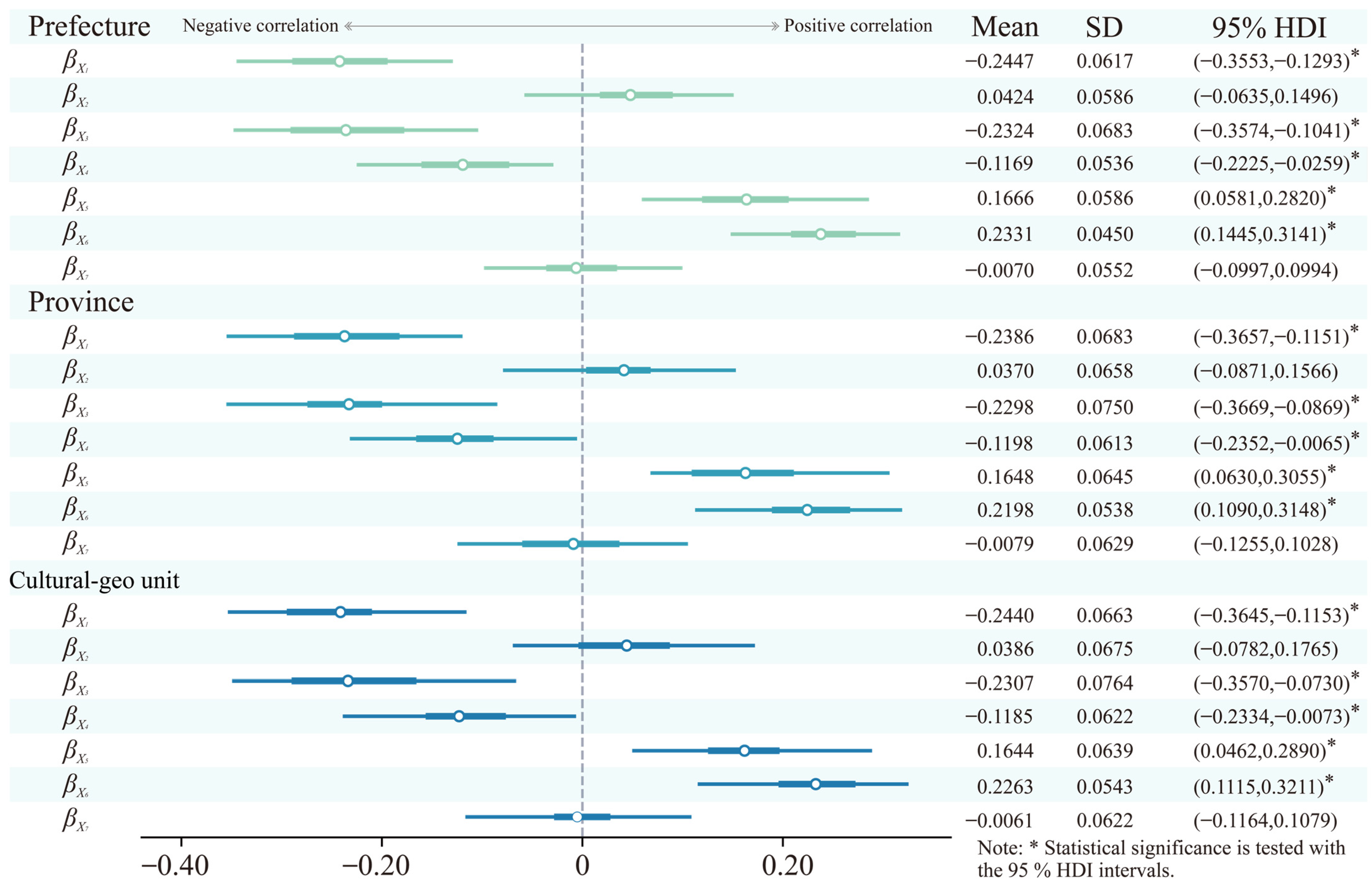
The posterior distributions of the regression coefficients for the seven feature variables at the overall level showed clear patterns of statistical significance. The mean values of β_X1, β_X2, β_X3, β_X4, β_X5, β_X6, and β_X7 were −0.240, 0.035, −0.233, −0.121, 0.161, 0.224, and −0.002, respectively, with corresponding standard deviations of 0.068, 0.061, 0.074, 0.060, 0.057, 0.050, and 0.061, respectively; the 95% highest density intervals (HDIs) were (−0.371, −0.111), (−0.088, 0.153), (−0.369, −0.080), (−0.235, −0.002), (0.049, 0.276), (0.129, 0.322), and (−0.115, 0.124), respectively. The relatively low standard deviations for all feature variables indicated that the uncertainty in parameter estimation was well controlled. X₁, X₃, and X₄ exhibited statistically significant negative effects on coupling, whereas X₅ and X₆ exhibited statistically significant positive effects. No evidence was found for a significant effect of X₂ or X₇, suggesting that their direct associations with coupling are weak and may instead operate indirectly through mediating variables.

Even under hyperprior constraints, differences between parameter groups were maintained through independent sampling (Figure 7). The five significant factors at the overall level remained significant across all three scales, reflecting consistency in their influence mechanisms. At the group level, the effect strengths of the variables displayed some differentiation. Specifically, the mean values of β_X1 were −0.2447, −0.2386, and −0.2440; β_X3 were −0.2324, −0.2298, and −0.2307; β_X4 were −0.1169, −0.1198, and −0.1185; β_X5 were 0.1666, 0.1648, and 0.1644; and β_X6 were 0.2331, 0.2198, and 0.2263. Notably, the interaction between GDP and population density had a negative effect, whereas the interaction with the share of the tertiary sector was positive. This suggests that different economic development trajectories may influence heritage coupling through either spatial restructuring or service-oriented pathways.

Figure 7. Posterior distributions of group-level regression coefficients. Different colors represent the three geographic levels, with all seven coefficients for each level shown in the same color.

Except for X₄, the remaining four significant variables reached their maximum effect strength at the prefecture-level scale. This pattern reflected the amplification of local factors at fine spatial units and the regionalized characteristics of heritage transmission. X₁, X₃, and X₆ exhibited the lowest effect strength at the provincial scale, forming a U-shaped distribution with relatively strong effects at the other two scales. By contrast, X₄ reached its maximum effect strength at the provincial scale, while X₅ showed a monotonically decreasing pattern. These differences indicated that the coupling characteristics of multi-scale geographic processes were influenced by distinct driving mechanisms. The provincial scale did not simply inherit the hierarchical changes in scale; specific inhibitory mechanisms may have systematically weakened or diluted certain coupling processes. The high effects observed at the prefecture-level scale reflected the direct influence of localized processes, whereas the rebound of effects at the cultural–geographical unit scale reflected the regulatory role of the overall cultural system on coupling processes. These findings deviated from the traditional assumption of diminishing scale effects [87] and revealed a nonlinear interaction pattern between administrative boundary effects and the continuity of geographic processes.

3.4. Causal Effect Estimation and Comparison

The mixed causal inference framework further refined observed correlations into model-based causal effect estimates, which necessarily rely on core assumptions such as model specification and instrumental-variable validity. Accordingly, the resulting causal effects should be interpreted as estimates conditional on these assumptions. Based on the combined validation of HBM significance and the strength of causal evidence, X₁ and X₅ were selected as the primary treatment variables, and X₃ and X₄ were used as robustness variables. The exploratory variables included mean annual precipitation (X₈), elevation (X₉), river network density (X₁₀), road network density (X₁₁), tertiary sector share (X₁₂), and slope gradient (X₁₃). At the prefecture-level scale, Conley–HAC standard errors were estimated for alternative bandwidths (Table 3). The significance levels of X₁, X₅, X₃, and X₄ remained unchanged, but under the baseline bandwidth, their standard errors changed by −2.7%, +5.6%, −1.9%, and −4.8%, respectively. Across the full bandwidth range, the maximum variation ranged from −5.1% to +9.5%. These patterns indicated that the core inferences were robust to plausible spatial correlation. The adaptive bandwidth achieved 75.2% node coverage, suggesting that this setting adequately captured the principal scale of inter-city spatial dependence. Overall, the causal inference model exhibited no material spatial dependence and, so, introducing an additional spatially structured component was unnecessary. Subsequently, we compared causal effect estimates from OLS and DML (Figure 8).

Table 3. Spatial robustness checks for causal estimates at the prefecture level.

Variable	SE/p	Conley 90.7 km (SE/p/ΔSE)	Conley 112.8 km (SE/p)	Conley 138.6 km (SE/p)
X1	0.0994/0.0001	0.0970/0.0001/−2.4%	0.0967/0.0001/−2.7%	0.0968/0.0001/−2.6%
X5	0.0563/0.0045	0.0583/0.0062/3.7%	0.0594/0.0071/5.6%	0.0616/0.0095/9.5%
X3	0.0875/0.0033	0.0859/0.0027/−1.8%	0.0858/0.0027/−1.9%	0.0854/0.0026/−2.4%
X4	0.0652/0.4955	0.0619/0.4728/−5.1%	0.0621/0.4742/−4.8%	0.0630/0.4800/−3.5%
Node Coverage	—	25.6%	50.0%	75.2%

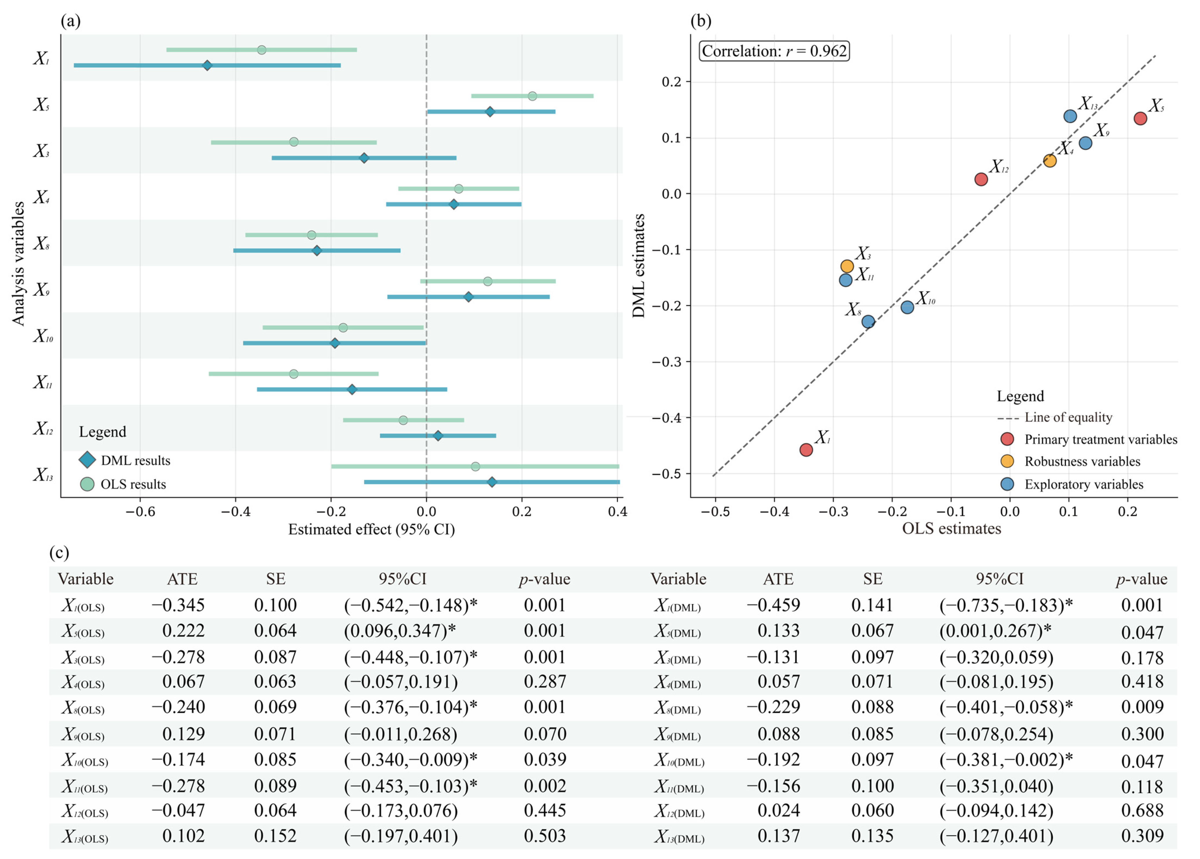
Figure 8. Causal effects of selected variables: comparison of OLS and DML estimates. (a) Causal effects of selected variables: OLS and DML estimates; (b) comparison of causal effect estimates: OLS and DML methods; (c) statistical summary of causal effect estimates. * Indicates statistical significance at the 5% level (p < 0.05).

X₁, X₅, X₈, and X₁₀ showed significant and robust causal effect estimates under both estimation strategies. X₁ exhibited a strong negative effect estimate, indicating that low-temperature regions were more conducive to maintaining heritage associations and traditional lifestyles. The ATEs were −0.345 and −0.459, with the latter representing a 33% increase in effect magnitude. This suggested that, after controlling for selection bias and confounding variables, temperature had a more pronounced negative impact on coupling intensity. X₅ showed a significant positive effect estimate, with ATEs of 0.222 and 0.133. The approximately 40% reduction in the latter effect may have resulted from DML’s control of the independent effects of water systems and roads, as well as their interactions with other infrastructure components. X₈ exhibited a robust negative effect estimate, with ATEs of −0.240 and −0.229, indicating that high precipitation negatively impacted heritage coupling. X₁₀ exhibited a significant negative effect estimate, with ATEs of −0.174 and −0.192. Its positive interaction with road networks suggested that the negative effect of water system density was reduced by road conditions. X₃ and X₁₁ only achieved significant effect estimates under OLS estimation, with ATEs of −0.278, potentially due to mediating variables [88]. X₄, X₉, X₁₂, and X₁₃ were not significant under either estimation strategy, indicating limited evidence for their independent causal effects.

The strong correlation between the OLS and DML estimates (r = 0.962) indicated high concordance between the two methods in identifying the direction and magnitude of effects. DML was particularly effective at controlling high-dimensional confounders and capturing nonlinear features, typically providing more conservative yet robust estimates [75]. For instance, DML amplified the negative effect of the primary treatment variable, X₁, while moderately attenuating the positive effect of X₅. As a parametric baseline method, OLS emphasized interpretability and computational efficiency, providing an intuitive linear approximation. The complementarity of the two methods offered an empirical basis for understanding the potential causal mechanisms underlying heritage coupling systems.

3.5. Heterogeneity Grouping and Differentiated Effects

The top five heterogeneity grouping strategies are presented in Table 4. Among them, the mean annual temperature grouped using K-means clustering (k = 2) achieved the highest overall score of 0.9810. This grouping strategy performed well across all three dimensions: statistical significance, effect size, and inter-group differences. The K-means binary grouping effectively identified critical thresholds [89] in temperature variation. This strategy aligned with the climatic differentiation observed in China and was suitable for revealing the differentiated mechanisms of influencing factors across distinct climate zones.

Table 4. Optimal heterogeneity grouping results.

Grouping Variable	Optimal Grouping Method	p-Value	Effect Size	Δμ	max(Δμ)	Composite Score
Annual temperature	K-means (k = 2)	1.71 × 10−13	0.9789	3.1728	3.2767	0.9810
NDVI	K-means (k = 2)	1.83 × 10−7	0.9671	3.2767	3.2767	0.9803
Annual temperature	Quartile extreme	1.26 × 10−7	0.9131	3.5932	3.5932	0.9479
Heritage density	K-means (k = 2)	4.93 × 10−9	0.9186	3.0819	3.2767	0.9393
Elevation	K-means (k = 2)	4.71 × 10−9	0.9054	3.0348	3.2767	0.9285

The differentiated robustness testing strategies for the three types of variables provided a credible basis for the heterogeneity analysis. For the primary treatment variables X₁ and X₅, the Δ_robust pass rates were 87.5% and 100%, respectively, indicating that their coefficients remained stable after most or all confounding variables were included. The Δ_norm values were 0.658 and 0.949, respectively, demonstrating substantial consistency between the two estimation methods. Notably, only X₅ passed the heterogeneity test, confirming its differentiated effect across groups (Table 5).

Table 5. Primary treatment variable robustness testing results.

Variable	Δrobust Pass Rate	Δnorm	Heterogeneity
X1	87.5%	0.658	×
X5	100%	0.949	✓

Note: ✓ indicates heterogeneity between groups; × indicates no significant heterogeneity.

The robustness variables X₃ and X₄ had Δ_robust pass rates of 100%, demonstrating high stability after controlling for confounding factors. Their Δ_norm values were 1.073 and 0.456, respectively, indicating statistical consistency between the two methods. However, neither variable passed the heterogeneity test (Table 6).

Table 6. Robustness variables robustness testing results.

Variable	Δrobust Pass Rate	Δnorm	Heterogeneity
X3	100%	1.073	×
X4	100%	0.456	×

Note: × indicates no significant heterogeneity.

The six exploratory variables exhibited pronounced differences in robustness characteristics (Table 7). According to the differentiated testing strategy, only the variables X₈, X₁₀, and X₁₁, which exhibited significant effects in the baseline model, were subjected to method consistency testing. X₈ exhibited the best overall performance, with a Δ_norm value of 0.104 and a Δ_robust pass rate of 75%, reflecting strong method consistency and stability. The fact that it passed the heterogeneity test confirmed significant effect differences across groups. For X₁₀ and X₁₁, the Δ_robust pass rates were 50% and 70%, respectively, and the Δ_norm values were 0.149 and 0.938, respectively. However, neither variable passed the heterogeneity test. For the baseline model variables X₉, X₁₂, and X₁₃, the Δ_robust values did not exceed 50%, with no heterogeneity observed.

Table 7. Exploratory variable robustness testing results.

Variable	Δrobust Pass Rate	Δnorm	Heterogeneity
X8	75%	0.104	✓
X9	50%	—	×
X10	50%	0.149	×
X11	75%	0.938	×
X12	0%	—	×
X13	50%	—	×

Note: Δ_norm is calculated only for significant variables. ✓ indicates heterogeneity between groups; × indicates no significant heterogeneity.

These results indicated that X₅ and X₈ exhibited significant heterogeneity. Although X₁ did not pass the heterogeneity test, its significant effect and Δ_robust pass rate of 87.5% suggested the possibility of a more complex pattern. Based on K-means clustering (k = 2) of the mean annual temperature, we focused on the heterogeneity mechanisms of X₅ and X₈ while retaining an exploratory analysis of X₁ (Figure 9).

Figure 9. Heterogeneity estimation under mean annual temperature grouping. (a) Grouping based on mean annual temperature; (b) forest plot comparing OLS and DML heterogeneous effects. * Indicates statistical significance at the 5% level (p < 0.05).

X₁ not only served as the basis for grouping but also exhibited differences in its effect on coupling. The OLS estimates indicated a significant negative effect estimate in low-temperature areas (ATE = −0.787), whereas the effect in high-temperature areas was nonsignificant. By contrast, the DML approach showed that neither region reached conventional significance levels. The I² values were 34.4% and 14.4% for the two methods, respectively, and the Q test did not detect any significant differences between the groups. This result suggested that temperature may exert a nonlinear influence on heritage coupling, although the evidence remains insufficient under the current dataset.

X₅ exhibited the strongest heterogeneity. Both methods showed a significant positive effect estimate in the low-temperature region (ATE = 0.429 and ATE = 0.431), while the effect was not significant in the high-temperature region. The I² values were 87.3% and 88.4%, and the Q test indicated very high between-group heterogeneity. These results suggested that well-developed transport and waterway networks may have been key to overcoming climatic constraints in low-temperature regions [90], facilitating the flow and integration of cultural elements. By contrast, in high-temperature regions, where climatic conditions were relatively favorable, the marginal contribution of transportation and waterways was markedly reduced.

X₈ also exhibited significant heterogeneity. Both methods showed a significant negative effect estimate in the low-temperature region (ATE = −0.910 and ATE = −0.782), whereas the effect was not significant in the high-temperature region. The I² values were 74.2% and 70.7%, and the Q test was significant. These findings indicated that the impact of precipitation on coupling was temperature-dependent. Precipitation heterogeneity reflected the role of climate in shaping the spatial patterns of agricultural civilizations and cultural forms [91]. In low-temperature regions, excessive precipitation may have suppressed heritage linkages through mechanisms such as hindering transportation and constraining social activities, whereas this suppressive effect was no longer significant in high-temperature regions.

It should be noted that heterogeneity identification depends on the grouping method and testing criteria. Inter-group inconsistencies represent statistical evidence obtained under specific strategies and do not completely negate underlying mechanisms. These results revealed the complex regulatory role of geographical factors in the cultural heritage coupling system under different temperature conditions. Temperature was found to directly affect heritage coupling and constrain the influence of other factors. Both X₅ and X₈ exerted significant effects in low-temperature regions, while their impacts weakened in high-temperature regions. This temperature-centered environmental regulation mechanism demonstrated that the influence of geographical factors on cultural heritage coupling did not operate independently but instead formed a differentiated network of interactive effects under specific environmental contexts.

4. Discussion

4.1. Interpretation of Driving Mechanisms from HBM and Causal Evidence

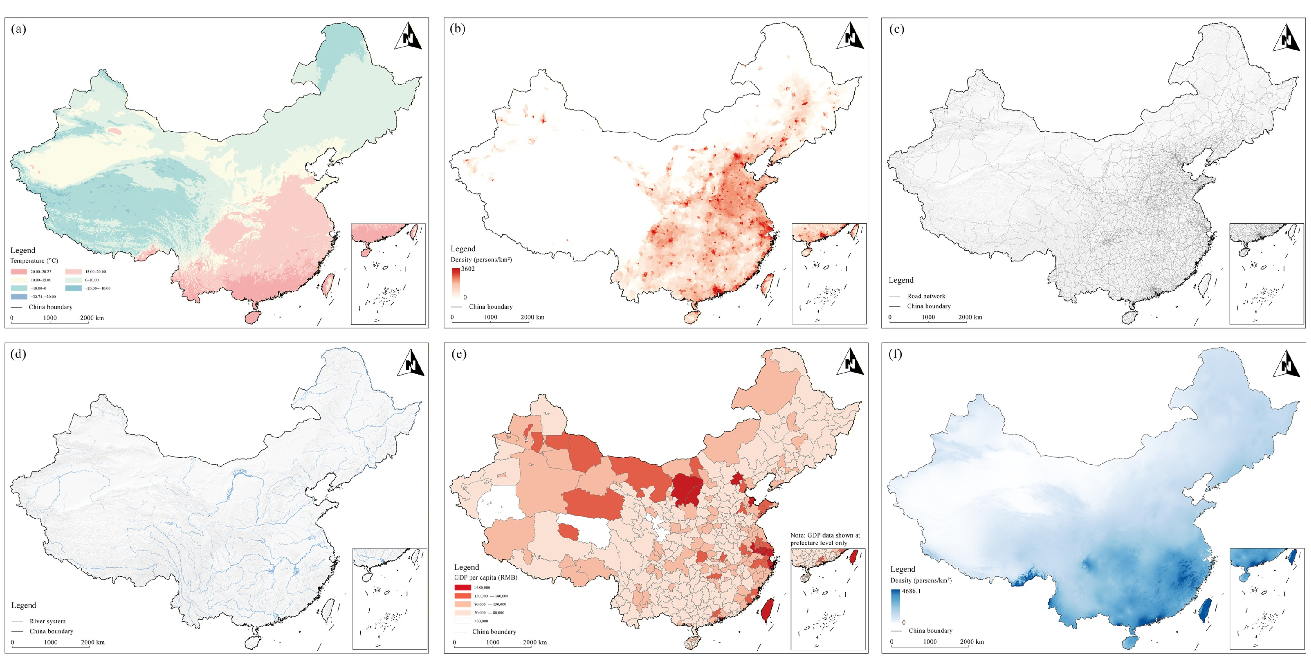
This study reveals the multi-scale driving mechanisms of spatial coupling between TCH and ICH in China by integrating HBM and causal inference methods. The progressive evidence chain, from correlation to model-based causal effect estimates and heterogeneity, provides multiple empirical foundations for understanding the complexity of heritage systems. Figure 10 illustrates the spatial distribution of the five core variables, facilitating an understanding of their geographical associations with degrees of coupling.

Figure 10. Spatial distribution of driving variables. (a) Mean annual temperature; (b) population density; (c) road network distribution; (d) water system distribution; (e) per capita GDP; (f) mean annual precipitation.

The significant negative effect estimate of X₁ indicates higher coupling intensity in low-temperature regions. Although the heterogeneity does not reach a statistically significant level, this result still reflects the nonlinear role of temperature. In China, temperature exhibits clear latitudinal and altitudinal gradients, with southern regions generally warmer than vast areas in the west and northeast. This spatial correspondence suggests that temperature, as a fundamental environmental variable, shapes heritage patterns by influencing human activity and cultural practices [92]. The underlying mechanism may lie in the tendency of low-temperature environments to form relatively enclosed geographic units, which consolidate community structures and cultural identities [93], thereby facilitating the co-transmission of both types of heritage. In the context of global warming, high temperatures may weaken the spatial linkage between heritage types by reshaping traditional lifestyles and increasing environmental pressures [94]. Notably, mean annual temperature also emerges as the optimal variable for heterogeneity grouping, supporting the foundational role of climatic conditions in heritage coupling systems.

X₃ and its interaction with per capita GDP (X₄) both exert significant negative effect estimates. Conventionally, areas with high population density often host rich heritage resources. For instance, migration and urban expansion in Jordan have shaped the multi-layered evolution of As-Salt’s architecture and cultural landscape [95]. However, our results indicate that in regions of high population concentration and economic prosperity in China, heritage coupling intensity tends to be lower. Using the ‘Hu Huanyong Line’ to delineate population density patterns, we observe that the eastern and southeastern regions display lower overall coupling than the western and northwestern regions. This decoupling phenomenon suggests that cultural transmission in modern societies is challenging, highlighting the need for integrated protection. Rapid urbanization may accelerate the spatial separation and cultural decoupling of the two heritage types by dismantling local cultural contexts [27]. TCH may relocate or disappear due to urban renewal, while ICH may lose its continuity as the linkage between traditional communities and heritage spaces weakens. In contrast to the inhibitory effect of X₄ on coupling, the interaction between per capita GDP and tertiary industry share (X₆) exhibits a significant positive effect estimate. Studies on cultural tourism coupling in the Beijing–Tianjin–Hebei urban agglomeration indicate that industrial restructuring and digital infrastructure are key drivers of integration [96]. This suggests that when economic development is accompanied by optimized heritage tourism and creative cultural industries, the heritage value chain can be restructured to actively connect both types of heritage. Such a shift implies that heritage protection can transform from a mere cost burden into a value-creating process, providing market-based pathways to support the coordinated development of heritage.

X₅ exhibits a robust positive effect estimate, showing significant heterogeneity between low- and high-temperature regions. Transportation networks and river systems form a collaborative network that serves as critical infrastructure for cultural exchange in relatively isolated cold environments, acting as traditional channels of cultural dissemination. This is essential for maintaining cultural connections between dispersed communities and heritage sites. By contrast, this effect is not significant in high-temperature regions with greater openness, suggesting that cultural transmission in these areas relies more on other mechanisms, such as tourism or institutional protection. Notably, river density (X₁₀) alone demonstrates a negative effect estimate in causal tests, indicating that overly dense river networks, in the absence of adequate transportation infrastructure, may isolate communities from heritage sites [97], thereby weakening the coupling degree. However, when interacting with road networks, it exhibits a significant positive effect estimate. Studies on the coupling between village cultural landscapes and socio-economic systems demonstrate that improving transportation accessibility facilitates the dual objectives of heritage protection and economic development [98]. The pattern of individual inhibition but interactive promotion highlights that road networks can mitigate the spatial fragmentation caused by river systems, thereby supporting the maintenance and dissemination of cultural activities and ultimately reinforcing the integration of TCH and ICH. The construction of interaction variables followed the collaborative logic of scientific elements based on indicator validation, allowing the estimation of synergistic effects that exceed individual contributions. This ensures that the causal evidence represents not only statistical signals but also underlying environmental linkages.

X₈ has a significant negative effect estimate, with significant heterogeneity. The negative impact of precipitation is significant in low-temperature regions, likely because the combination of cold and high precipitation creates a harsh natural environment that amplifies geographical isolation. Concentrated rainfall and spring floods can cause structural degradation of heritage in cold areas and prolong restoration cycles [99], disrupting the heritage transmission chain. Frequent precipitation and flooding make heritage protection more difficult and hinder human mobility and cultural exchange, ultimately reducing cross-regional cultural integration. Conversely, this effect is not significant in high-temperature regions, which may benefit from long-established adaptive mechanisms such as moisture-resistant architecture and water transportation systems in southern areas. These differentiated effects reflect how environmental constraints translate into cultural outcomes [100]. Distinct cultural systems, such as those of Jiangnan and Lingnan, have evolved in warm and humid conditions, exemplifying human societies’ adaptive transformation of nature.

4.2. Differentiated Governance Strategies for Heritage Protection

Multi-level evidence provides valuable insights into heritage conservation and regional governance (Table 8). Given the central role of climate and its moderating effects, differentiated, climate-adaptive conservation strategies should be developed based on coupling relationships. Heritage impact mechanisms exhibit significant differentiation across varying temperature contexts, as stone and timber materials demonstrate different material-specific thresholds to climatic stress [101]. Combining the positive effects of road–water interaction with the negative effects of water system density, water management should proceed in parallel with accessibility infrastructure development. In low-temperature regions, the synergistic effects of road–water interconnection should be fully utilized, with integrated transport projects promoting the clustered development of heritage sites within cultural corridors [102]. In areas with dense water systems but limited land transport, priority should be given to improving terrestrial infrastructure or enhancing waterway services. This helps to prevent spatial fragmentation from reducing coupling degrees. Key improvements should focus on enhancing the landscapes of vernacular communities and making heritage more accessible, as well as on strengthening the interaction between heritage and daily life. In high-temperature or climate-vulnerable areas, priority should be given to heritage risk assessment and protective restoration. At the same time, cultural transmission mechanisms or digital platforms should be established to reduce the impacts of climatic stress on coupling degrees.

Table 8. Key findings and policy recommendations.

Variable and Effect Direction	Theoretical Mechanism	Policy Recommendations	Implementation Scale
X1: Negative	Low temperature enhances geographic enclosure and cultural cohesion	Integrate climate adaptation into heritage planning; prioritize protection in cold regions	Provincial/cultural–geographical unit
X3: Negative	Population agglomeration accelerates urbanization and deconstructs vernacular culture	Embed heritage buffer zones in urban areas; conduct heritage impact assessments	Prefecture level
X4: Negative	Compounded effects of economy and population exacerbate cultural decoupling risks	Prevent cultural decoupling from aggressive urbanization; establish holistic protection mechanisms	Prefecture–provincial combined
X5: Positive	Infrastructure complementarity generates synergistic effects	Develop cultural–tourism transport corridors; prioritize road connectivity improvements	Provincial/cultural–geographical unit
X6: Positive	Industrial restructuring enhances heritage value chains	Promote tourism and creative industries; balance commercialization with authenticity protection	Prefecture/provincial
X8: Negative	Low temperature and precipitation compound geographic isolation and structural degradation	Strengthen moisture and flood prevention facilities in cold-humid regions; establish adaptive protection systems	Provincial/cultural–geographical unit
X10: Negative	Road networks can mitigate spatial fragmentation caused by dense river networks	Coordinate waterway management with accessibility improvements	Prefecture/provincial

Regarding the negative effects in densely populated and economically developed areas, excessive urbanization leading to cultural decoupling should be prevented. Heritage conservation buffer zones should be incorporated into urban renewal and land planning to maintain connections between heritage and daily life [103]. Cultural activity circles or subsidy mechanisms should be established to encourage local culture and traditional crafts. Simultaneously, heritage impact assessments and cultural space protection clauses can be incorporated into urban construction to prevent heritage spatial separation caused by development. The positive effects of economic structural transition toward tertiary industries indicate that heritage conservation can be transformed from cost consumption into value generation through the development of cultural industries and heritage tourism [104]. Cultural industrial parks can be established to promote spatial clustering and reproduction while mitigating the risks of homogenization caused by over-commercialization.

Differentiated governance frameworks are crucial for formulating and implementing heritage conservation policy [105]. Prefecture-level scales are suitable for undertaking specific infrastructure construction and community cultural conservation projects. Provincial scales can play coordinating roles across administrative regions and integrate resources. Cultural–geographical unit scales should respect the authenticity of cultural ecosystems by conducting conservation and transmission planning centered on cultural spaces. Thus, a three-tier indicator system encompassing ‘risk assessment–accessibility–socioeconomic structure’ is recommended, with performance indicators such as coupling degree changes and cultural activity participation rates established for process management and evaluation. Through multi-scale collaborative governance mechanisms, regional cultural balanced development and factor sharing can be promoted more effectively, facilitating heritage activation and socioeconomic synergy.

5. Conclusions

This study established an integrated analytical framework for coupling degree assessment that combines multi-scale geographic units, Bayesian modeling, and causal inference. A coupling degree measurement system for heritage was constructed at the prefecture-level, provincial, and cultural–geographical unit scales, based on the MCLQ index. The key driving variables were then identified using the HBM. Bayesian statistics and causal identification tools were employed together to screen potential variables and categorize them hierarchically. Subsequently, the model-based causal effects were estimated using a differentiated hybrid framework. Following robustness checks, optimal grouping methods were applied to capture heterogeneity in factor effects across groups, and the spatial distribution patterns of heritage coupling and the heterogeneity of its driving mechanisms in China were systematically examined. The main empirical findings are as follows:

(1)

Heritage coupling patterns showed scale dependence and cultural cohesion. The proportion of strongly coupled areas decreased from the prefecture-level to the provincial scale, consistent with typical spatial attenuation patterns, but rose noticeably at the cultural–geographical unit scale. This anomaly revealed a cohesive effect for China’s cultural system that transcended administrative boundaries.

(2)

The HBM identified five critical drivers and their differentiated impacts. X₁, X₃, and X₄ exhibited significant negative effects, whereas X₅ and X₆ showed significant positive effects. Except for X₄, the effect intensity of the remaining four variables peaked at the prefecture-level scale and generally diminished at the provincial scale. This suggested the presence of a suppressive mechanism at the provincial level, which attenuated the effects of these factors.

(3)

The hybrid causal inference framework provided model-based causal estimation evidence for four key variables. Through dual testing with OLS and DML verification, X₁, X₈, and X₁₀ displayed significant negative causal effect estimates, while X₅ exhibited a significant positive causal effect estimate.

(4)

Heterogeneity analysis detected differentiated causal effects for two variables. In K-means clustering (k = 2) based on annual average temperature, the positive effect estimate of X₅ and the negative effect estimate of X₈ were significant in the low-temperature group but not in the high-temperature group. This indicated that temperature conditions moderated the driving mechanisms of heritage coupling.

By organically integrating data-driven HBM with logic-driven causal inference and incorporating a wide range of geographic and social variables, this study uncovers multiple driving mechanisms of heritage coupling and their heterogeneity. However, several empirical limitations exist regarding causal interpretation. Firstly, some factors involving potential mediating pathways could not be incorporated into the hybrid framework. Secondly, it was not possible to continuously explore the temporal evolution of the heritage coupling system due to constraints in historical data. Spatial units partially reflect institutional and social processes rather than purely neutral natural variables, and thus cannot be completely distinguished from cultural dynamics. Furthermore, some instrumental variables with limited strength suggest potential weak instrument bias. This study presents optimal estimates based on the current model assumptions and data conditions rather than definitive causal relationships obtained under experimental conditions. Future research could employ quasi-natural experimental designs, spatiotemporal panels and multi-scenario grouping strategies to improve identification capabilities. Structural equation modeling could also be applied to clarify theoretical causal pathways and mediation testing. The analytical framework could incorporate qualitative elements such as participatory geographic information systems, policies, and community behaviors, thereby enabling a deeper exploration of the differences and integration pathways between official recognition and local needs. From a practical perspective, this study primarily aimed to validate and deepen causal understanding of the intrinsic drivers of heritage coupling, thus providing a methodological reference for the conservation of cultural heritage at multiple scales.

References

1. Shen, W.; Chen, Y.L.; Cao, W.W.; Yu, R.Y.; Rong, P.J.; Cheng, J.L. Spatial pattern and its influencing factors of national-level cultural heritage in China. npj Herit. Sci. 2024, 12, 384. [Google Scholar] [CrossRef]
2. Malik, U.S.; Micoli, L.L.; Caruso, G.; Gabriele, G. Integrating quantitative and qualitative analysis to evaluate digital applications in museums. J. Cult. Herit. 2023, 62, 304–313. [Google Scholar] [CrossRef]
3. Guttormsen, T.S.; Skrede, J.; Guzman, P.; Fouseki, K.; Bonacchi, C.; Pastor Pérez, A. Assemblage urbanism: The role of heritage in urban placemaking. J. Cult. Herit. Manag. Sustain. Dev. 2023. ahead-of-print. [Google Scholar] [CrossRef]
4. Taylor, K. The Historic Urban Landscape paradigm and cities as cultural landscapes. Challenging orthodoxy in urban conservation. Landsc. Res. 2016, 41, 471–480. [Google Scholar] [CrossRef]
5. Monteiro, V.; Painho, M.; Vaz, E. Is the heritage really important? A theoretical framework for heritage reputation using citizen sensing. Habitat Int. 2015, 45, 156–162. [Google Scholar] [CrossRef]
6. Ferretti, V.; Comino, E. An integrated framework to assess complex cultural and natural heritage systems with Multi-Attribute Value Theory. J. Cult. Herit. 2015, 16, 688–697. [Google Scholar] [CrossRef]
7. Ripp, M.; Gustafsson, C.; Jones, Z.; Majumdar, S.; Ginzarly, M. Historic Urban Landscapes and Heritage Systems as the Basis for Sustainable Urban Development. Land 2025, 14, 1783. [Google Scholar] [CrossRef]
8. Taylor, K.; Lennon, J. Cultural landscapes: A bridge between culture and nature? Int. J. Herit. Stud. 2011, 17, 537–554. [Google Scholar] [CrossRef]
9. Zhang, Z.W.; Cui, Z.; Fan, T.S.; Ruan, S.Y.; Wu, J.M. Spatial distribution of intangible cultural heritage resources in China and its influencing factors. Sci. Rep. 2024, 14, 4960. [Google Scholar] [CrossRef] [PubMed]
10. Xue, Q.M.; Huang, Y.H. The spatial relationship and influence mechanism of traditional villages and intangible cultural heritage: A case study of the upper reaches of the Yellow River Basin. Hum. Soc. Sci. Commun. 2025, 12, 142. [Google Scholar] [CrossRef]
11. Li, C.; Qian, Y.Y.; Li, Z.K.; Tong, T. Identifying factors influencing the spatial distribution of minority cultural heritage in Southwest China. npj Herit. Sci. 2024, 12, 117. [Google Scholar] [CrossRef]
12. Ma, Q.B.; Liu, T.T.; Yang, Z.; Zhang, S.; Zhang, X.Y.; Sun, M.N.; Hou, X.X. The spatio-temporal distribution and influencing factors of cave temples and stone carvings in China. npj Herit. Sci. 2025, 13, 311. [Google Scholar] [CrossRef]
13. Feng, Y.; Wei, H.; Huang, Y.; Li, J.W.; Mu, Z.Q.; Kong, D.Z. Spatiotemporal evolution characteristics and influencing factors of traditional villages: The Yellow River Basin in Henan Province, China. npj Herit. Sci. 2023, 11, 97. [Google Scholar] [CrossRef]
14. Liu, E.L.; Zhang, J.; Chi, H.N. Spatial distribution and driving factors of Chinese dragon and lion dance athletes based on GIS. Heliyon 2024, 10, e23409. [Google Scholar] [CrossRef] [PubMed]
15. Dong, B.L.; Bai, K.; Sun, X.L.; Wang, M.T.; Liu, Y. Spatial distribution and tourism competition of intangible cultural heritage: Take Guizhou, China as an example. npj Herit. Sci. 2023, 11, 64. [Google Scholar] [CrossRef]
16. Chen, W.X.; Yang, Z.; Yang, L.Y.; Wu, J.H.; Bian, J.J.; Zeng, J.; Liu, Z.L. Identifying the spatial differentiation factors of traditional villages in China. npj Herit. Sci. 2023, 11, 149. [Google Scholar] [CrossRef]
17. Jiang, L.W.; Cai, J.; Fan, Y.L. Spatiotemporal Distribution and Heritage Corridor Construction of Vernacular Architectural Heritage in the Cao’e River, Jiaojiang River, and Oujiang River Basin. Land 2025, 14, 1484. [Google Scholar] [CrossRef]
18. Zhang, W.Y.; Ma, L.H.; Xu, J.Y.; Peng, Y.J. Spatial–temporal distribution characteristics and influencing factors of immovable cultural heritage in Hubei, China. Sci. Rep. 2025, 15, 24570. [Google Scholar] [CrossRef]
19. Zhang, J.H.; Jiang, L.; Wang, X.Q.; Chen, Z.L.; Xu, S.B. A Study on the Spatiotemporal Aggregation and Corridor Distribution Characteristics of Cultural Heritage: The Case of Fuzhou, China. Buildings 2024, 14, 121. [Google Scholar] [CrossRef]
20. Zhu, L.T.; Li, Z.W.; Su, H.M.; Wang, X. Temporal and spatial distribution of ancient sites in Shaanxi Province using geographic information systems (GIS). npj Herit. Sci. 2021, 9, 121. [Google Scholar] [CrossRef]
21. Laguna-Palma, D.; Palacios, O.; Mokránová, K. Assessing the risks of northeastern African archaeological heritage and their relationship to human–environmental processes: A Bayesian network approach. World Archaeol. 2023, 55, 366–381. [Google Scholar] [CrossRef]
22. Zhang, S.R.; Chi, L.; Zhang, T.Y.; Ju, H.R. Spatial pattern and influencing factors of land border cultural heritage in China. npj Herit. Sci. 2023, 11, 187. [Google Scholar] [CrossRef]
23. Liu, W.X.; Xue, Y.; Shang, C. Spatial distribution analysis and driving factors of traditional villages in Henan province: A comprehensive approach via geospatial techniques and statistical models. npj Herit. Sci. 2023, 11, 185. [Google Scholar] [CrossRef]
24. Pang, L.; Wu, L.N. Distribution characteristics and influencing factors of Intangible Cultural Heritage in Beijing-Tianjin-Hebei. npj Herit. Sci. 2023, 11, 19. [Google Scholar] [CrossRef]
25. Liu, S.; Ge, J.; Bai, M.; Yao, M.; Zhu, Z.N. Uncovering the factors influencing the vitality of traditional villages using POI (point of interest) data: A study of 148 villages in Lishui, China. npj Herit. Sci. 2023, 11, 123. [Google Scholar] [CrossRef]
26. Du, Y.X.; Chen, L.; Xu, J.Y. Interactive effects of intangible cultural heritage and tourism development: A study based on the data panel PVAR model and coupled coordination model. npj Herit. Sci. 2024, 12, 401. [Google Scholar] [CrossRef]
27. Yan, L.; Shen, X.; Liu, P.L. Spatiotemporal evolution of the coupling coordination between inheritance of local culture and new-style urbanization in China. npj Herit. Sci. 2022, 10, 73. [Google Scholar] [CrossRef]
28. Huser, R.; Opitz, T.; Wadsworth, J.L. Modeling of spatial extremes in environmental data science: Time to move away from max-stable processes. Environ. Data Sci. 2025, 4, e3. [Google Scholar] [CrossRef]
29. Fiorucci, M.; Khoroshiltseva, M.; Pontil, M.; Traviglia, A.; Del Bue, A.; James, S. Machine Learning for Cultural Heritage: A Survey. Pattern Recognit. Lett. 2020, 133, 102–108. [Google Scholar] [CrossRef]
30. Zhuang, Y. Environmental Foundations to the Rise of Early Civilisations in China; Cambridge University Press: Cambridge, UK, 2024; pp. 23–79. [Google Scholar]
31. Wang, F.L.; Zhang, T.Y.; Zhang, S.R. MGWR reveals scale heterogeneity shaping intangible cultural heritage distribution in China. npj Herit. Sci. 2025, 13, 367. [Google Scholar] [CrossRef]
32. Guo, Y.; Yan, J.Y.; Wang, Z.B.; Li, J.X. Spatial Dataset of 3610 Items of China’s National Intangible Cultural Heritage in Five Packages. J. Glob. Change Data Discov. 2022, 6, 257–264. [Google Scholar] [CrossRef]
33. Dong, L.B.; Bettinger, P.; Liu, Z.G. Stand spatial structural diversity: Developing and validating a novel index. For. Ecol. Manag. 2024, 569, 122157. [Google Scholar] [CrossRef]
34. Ma, W.; Zhao, C. China Extreme and Average Temperature Index Dataset (1961–2012); National Tibetan Plateau/Third Pole Environment Data Center: Beijing, China, 2024. [Google Scholar] [CrossRef]
35. Peng, S.Z.; Ding, Y.X.; Liu, W.Z.; Li, Z. 1 km monthly temperature and precipitation dataset for China from 1901 to 2017. Earth Syst. Sci. Data 2019, 11, 1931–1946. [Google Scholar] [CrossRef]
36. Dong, J.W.; Zhou, Y.; You, N.S.; Cheng, C.; Yang, J.L. China 30 m Annual Maximum NDVI Dataset from 2000 to 2022; National Ecosystem Science Data Center: Beijing, China, 2021; (In Chinese). [Google Scholar] [CrossRef]
37. Yang, J.; Dong, J.; Xiao, X.; Dai, J.; Wu, C.; Xia, J.; Zhao, G.; Zhao, M.; Li, Z.; Zhang, Y.; et al. Divergent shifts in peak photosynthesis timing of temperate and alpine grasslands in China. Remote Sens. Environ. 2019, 233, 111395. [Google Scholar] [CrossRef]
38. WorldPop; Columbia University. Global High Resolution Population Denominators Project—Funded by The Bill and Melinda Gates Foundation (OPP1134076); University of Southampton: Southampton, UK, 2018. [Google Scholar] [CrossRef]
39. Tawakuli, A.; Havers, B.; Gulisano, V.; Kaiser, D.; Engel, T. Survey: Time-series data preprocessing: A survey and an empirical analysis. J. Eng. Res. 2025, 13, 674–711. [Google Scholar] [CrossRef]
40. Goswami, T.; Sinha, G.R. Statistical Modeling in Machine Learning: Concepts and Applications; Elsevier: Amsterdam, The Netherlands, 2022; pp. 287–306. [Google Scholar] [CrossRef]
41. Atkinson, A.C.; Riani, M.; Corbellini, A. The Box–Cox Transformation: Review and Extensions. Stat. Sci. 2021, 36, 239–255. [Google Scholar] [CrossRef]
42. Demircioğlu, A. The effect of feature normalization methods in radiomics. Insights Imaging 2024, 15, 2. [Google Scholar] [CrossRef]
43. Rosik, P.; Wójcik, J. Transport infrastructure and regional development: A survey of literature on wider economic and spatial impacts. Sustainability 2022, 15, 548. [Google Scholar] [CrossRef]
44. Crits-Christoph, P.; Gallop, R.; Gaines, A.; Rieger, A.; Connolly Gibbons, M.B. Instrumental variable analyses for causal inference: Application to multilevel analyses of the alliance–outcome relation. Psychother. Res. 2018, 30, 53–67. [Google Scholar] [CrossRef]
45. Ginzarly, M.; Houbart, C.; Teller, J. The Historic Urban Landscape approach to urban management: A systematic review. Int. J. Herit. Stud. 2018, 25, 999–1019. [Google Scholar] [CrossRef]
46. Li, Y.F.; Li, Y.; Zhou, Y.; Shi, Y.L.; Zhu, X.D. Investigation of a coupling model of coordination between urbanization and the environment. J. Environ. Manag. 2012, 98, 127–133. [Google Scholar] [CrossRef] [PubMed]
47. Diener, A.C.; Hagen, J. Geographies of place attachment: A place-based model of materiality, performance, and narration. Geogr. Rev. 2020, 112, 171–186. [Google Scholar] [CrossRef]
48. Pan, Z.; Chen, Y.L.; Huang, Y.H.; Zheng, L. The vernacular cultural landscape in traditional villages: Global hotspots, emerging trends, and a case study of China’s Qilu cultural district. Front. Earth Sci. 2024, 12, 1511292. [Google Scholar] [CrossRef]
49. Liu, B.B.; Wu, C.; Xu, W.X.; Shen, Y.N.; Tang, F.L. Emerging trends in GIS application on cultural heritage conservation: A review. npj Herit. Sci. 2024, 12, 139. [Google Scholar] [CrossRef]
50. Leslie, T.F.; Kronenfeld, B.J. The Colocation Quotient: A New Measure of Spatial Association Between Categorical Subsets of Points. Geogr. Anal. 2011, 43, 306–326. [Google Scholar] [CrossRef]
51. Xie, J.F.; Zhang, J.; Yang, Z.N.; Yu, T.F.; Xie, Y. Characterizing the spatial organization of urban functions using a distance-based colocation quotient approach: With special reference to Beijing. Habitat Int. 2025, 163, 103474. [Google Scholar] [CrossRef]
52. Pierce, J.; Martin, D.G.; Murphy, J.T. Relational place-making: The networked politics of place. Trans. Inst. Br. Geogr. 2010, 36, 54–70. [Google Scholar] [CrossRef]
53. Yu, Y.; Wang, J. Crouching the tiger, or hiding the dragon? scale in China’s heritage production. Built Herit. 2024, 8, 11. [Google Scholar] [CrossRef]
54. Tian, Y.S.; Kong, X.S.; Liu, Y.L. Combining weighted daily life circles and land suitability for rural settlement reconstruction. Habitat Int. 2018, 76, 1–9. [Google Scholar] [CrossRef]
55. Li, B.L.; Lu, Y.F.; Li, Y.D.; Zuo, H.Y.; Ding, Z.Q. Research on the spatiotemporal distribution characteristics and accessibility of traditional villages based on geographic information systems—A case study of shandong province, China. Land 2024, 13, 1049. [Google Scholar] [CrossRef]
56. Wang, L.; Zhang, F.F.; Zang, Y.Z.; Duan, J. Understanding the Regional Integration Process from the Perspective of Agglomeration and Urban Networks: Case Study in Central China. Int. J. Environ. Res. Public Health 2022, 19, 12834. [Google Scholar] [CrossRef] [PubMed]
57. Su, H.R.; Wang, Y.W.; Zhang, Z.; Dong, W. Characteristics and Influencing Factors of Traditional Village Distribution in China. Land 2022, 11, 1631. [Google Scholar] [CrossRef]
58. Kaplan, N.; Omer, I. Multiscale Accessibility—A New Perspective of Space Structuration. Sustainability 2022, 14, 5119. [Google Scholar] [CrossRef]
59. Wang, M.Y.; Pan, S.J.X.; Tao, Y.Q.; Sun, H.L.; Li, X.Y. Hierarchical Bayesian modelling of quasi-region-specific soil porosity. Ocean Eng. 2022, 266, 113052. [Google Scholar] [CrossRef]
60. Jia, X.Y.; Sedehi, O.; Papadimitriou, C.; Katafygiotis, L.S.; Moaveni, B. Nonlinear model updating through a hierarchical Bayesian modeling framework. Comput. Meth. Appl. Mech. Eng. 2022, 392, 114646. [Google Scholar] [CrossRef]
61. Yu, D.L.; Fang, C.L. How neighborhood characteristics influence neighborhood crimes: A Bayesian hierarchical spatial analysis. Int. J. Environ. Res. Public Health. 2022, 19, 11416. [Google Scholar] [CrossRef]
62. Rittirong, J.; Bryant, J.; Aekplakorn, W.; Prohmmo, A.; Sunpuwan, M. Obesity and occupation in Thailand: Using a Bayesian hierarchical model to obtain prevalence estimates from the National Health Examination Survey. BMC Public Health 2021, 21, 914. [Google Scholar] [CrossRef]
63. Veenman, M.; Stefan, A.M.; Haaf, J.M. Bayesian hierarchical modeling: An introduction and reassessment. Behav. Res. Methods 2023, 56, 4600–4631. [Google Scholar] [CrossRef]
64. Gelman, A. Prior distributions for variance parameters in hierarchical models (comment on article by Browne and Draper). Bayesian Anal. 2006, 1, 515–534. [Google Scholar] [CrossRef]
65. Polson, N.G.; Scott, J.G. On the half-Cauchy prior for a global scale parameter. Bayesian Anal. 2012, 7, 887–902. [Google Scholar] [CrossRef]
66. Roy, V. Convergence Diagnostics for Markov Chain Monte Carlo. Annu. Rev. Stat. Appl. 2020, 7, 387–412. [Google Scholar] [CrossRef]
67. Dias, F.; Suhadolnik, N.; Camargo, H.; Da Silva, S. Predicting the pulse of the Amazon: Machine learning insights into deforestation dynamics. J. Environ. Manag. 2024, 362, 121359. [Google Scholar] [CrossRef] [PubMed]
68. Karunasingha, D.S.K. Root mean square error or mean absolute error? Use their ratio as well. Inf. Sci. 2022, 585, 609–629. [Google Scholar] [CrossRef]
69. Martin, O. Bayesian Analysis with Python: A Practical Guide to Probabilistic Modeling; Packt Publishing Ltd.: Birmingham, UK, 2024; pp. 152–154. [Google Scholar]
70. Ahmad, S.; Batool, A.; Ali, Z. Spatial predictive analysis of drought duration in relation to climate change using interpolation techniques. Stoch. Environ. Res. Risk Assess. 2025, 39, 639–656. [Google Scholar] [CrossRef]
71. Anselin, L.; Syabri, I.; Kho, Y. GeoDa: An introduction to Spatial Data Analysis; Springer: Berlin/Heidelberg, Germany, 2009; pp. 73–89. [Google Scholar] [CrossRef]
72. Anselin, L. An Introduction to Spatial Data Science with GeoDa: Volume 1: Exploring Spatial Data; Chapman and Hall/CRC: New York, NY, USA, 2024; pp. 176–388. [Google Scholar] [CrossRef]
73. Baiardi, A.; Naghi, A.A. The value added of machine learning to causal inference: Evidence from revisited studies. Econom. J. 2024, 27, 213–234. [Google Scholar] [CrossRef]
74. Hünermund, P.; Louw, B.; Caspi, I. Double machine learning and automated confounder selection: A cautionary tale. J. Causal Inference 2023, 11, 20220078. [Google Scholar] [CrossRef]
75. Moccia, C.; Moirano, G.; Popovic, M.; Pizzi, C.; Fariselli, P.; Richiardi, L.; Ekstrøm, C.T.; Maule, M. Machine learning in causal inference for epidemiology. Eur. J. Epidemiol. 2024, 39, 1097–1108. [Google Scholar] [CrossRef]
76. Kelejian, H.H.; Prucha, I.R. HAC estimation in a spatial framework. J. Econom. 2007, 140, 131–154. [Google Scholar] [CrossRef]
77. Fitzenberger, B.; Mena, G.; Nimczik, J.; Sunde, U. Personality traits across the life cycle: Disentangling age, period and cohort effects. Econ. J. 2022, 132, 2141–2172. [Google Scholar] [CrossRef]
78. Borenstein, M. Avoiding common mistakes in meta-analysis: Understanding the distinct roles of Q, I-squared, tau-squared, and the prediction interval in reporting heterogeneity. Res. Synth. Methods 2023, 15, 354–368. [Google Scholar] [CrossRef] [PubMed]
79. Lu, X.; White, H. Robustness checks and robustness tests in applied economics. J. Econom. 2014, 178, 194–206. [Google Scholar] [CrossRef]
80. Wang, F.F.; Chen, X.; Xue, F. A review of Bayesian spatiotemporal models in spatial epidemiology. ISPRS Int. J. Geo Inf. 2024, 13, 97. [Google Scholar] [CrossRef]
81. De, C.C.; d’Haultfoeuille, X. Two-way fixed effects estimators with heterogeneous treatment effects. Am. Econ. Rev. 2020, 110, 2964–2996. [Google Scholar] [CrossRef]
82. MacKinno, J.G.; Nielsen, M.Ø.; Webb, M.D. Cluster-robust inference: A guide to empirical practice. J. Econom. 2023, 232, 272–299. [Google Scholar] [CrossRef]
83. Lakens, D. Calculating and reporting effect sizes to facilitate cumulative science: A practical primer for t-tests and ANOVAs. Front. Psychol. 2013, 4, 863. [Google Scholar] [CrossRef] [PubMed]
84. Maher, J.M.; Markey, J.C.; Ebert-May, D. The Other Half of the Story: Effect Size Analysis in Quantitative Research. CBE Life Sci. Educ. 2013, 12, 345–351. [Google Scholar] [CrossRef]
85. Qian, X.Y.; Yu, Y.; Liu, R.J. The Spatial Relationship Characteristics and Differentiation Causes Between Traditional Villages and Intangible Cultural Heritage in China. Buildings 2025, 15, 2094. [Google Scholar] [CrossRef]
86. Kamath, A.; Poojari, S.; Varsha, K. Assessing the robustness of normality tests under varying skewness and kurtosis: A practical checklist for public health researchers. BMC Med. Res. Methodol. 2025, 25, 206. [Google Scholar] [CrossRef]
87. Wang, W.L.; Wang, R.; Lu, Y.Y.; Meng, Y.Y.; Zhou, Z. A novel spatial heterogeneity decay model for depicting scale-effects in urban land. GISci. Remote Sens. 2025, 62, 2547122. [Google Scholar] [CrossRef]
88. Zuo, S.Z.; Ghosh, D.; Ding, P.; Yang, F. Mediation Analysis with the Mediator and Outcome Missing Not at Random. J. Am. Stat. Assoc. 2024, 120, 794–804. [Google Scholar] [CrossRef]
89. Ikotun, A.M.; Ezugwu, A.E.; Abualigah, L.; Abuhaija, B.; Heming, J. K-means clustering algorithms: A comprehensive review, variants analysis, and advances in the era of big data. Inf. Sci. 2023, 622, 178–210. [Google Scholar] [CrossRef]
90. Antonson, H.; Buckland, P.; Nyqvist, R. A society ill-equipped to deal with the effects of climate change on cultural heritage and landscape: A qualitative assessment of planning practices in transport infrastructure. Clim. Change 2021, 166, 18. [Google Scholar] [CrossRef]
91. Abebaw, S.E. A Global Review of the Impacts of Climate Change and Variability on Agricultural Productivity and Farmers’ Adaptation Strategies. Food Sci. Nutr. 2025, 13, e70260. [Google Scholar] [CrossRef]
92. Li, J.C.; Han, L.Y.; Zhang, G.M.; Su, Z.Z.; Zhao, Y.F. Temporal-spatial variations of human settlements in relation to environment change during the Longshan culture and Xia-Shang periods in Shanxi Province, China. Quat. Int. 2017, 436, 129–137. [Google Scholar] [CrossRef]
93. Rubin, S.E.; Mørch, I.; Olsen, N.; Nørtoft, K. Important intergenerational transmission of knowledge in promotion of well-being and cultural identity in Greenland. Int. J. Circumpolar Health 2024, 83, 2420479. [Google Scholar] [CrossRef] [PubMed]
94. Maldonado-Erazo, C.P.; Álvarez-García, J.; Río-Rama, M.d.l.C.d.; Durán-Sánchez, A. Scientific Mapping on the Impact of Climate Change on Cultural and Natural Heritage: A Systematic Scientometric Analysis. Land 2021, 10, 76. [Google Scholar] [CrossRef]
95. Cotella, V.A.; Aburamadan, R.; Di Perna, E. HBIM applications in the world heritage city of as-salt, Jordan: Architecture as a reflection of cultural diversity shaped by migratory flows. Digit. Appl. Archaeol. Cult. Herit. 2025, 37, e00418. [Google Scholar] [CrossRef]
96. Du, H.F.; Liu, J.G. Exploring Spatial–Temporal Coupling and Its Driving Factors of Cultural and Tourism Industry in the Beijing–Tianjin–Hebei Urban Agglomeration, China. Sustainability 2025, 17, 890. [Google Scholar] [CrossRef]
97. Fuller, M.R.; Doyle, M.W.; Strayer, D.L. Causes and consequences of habitat fragmentation in river networks. Ann. N. Y. Acad. Sci. 2015, 1355, 31–51. [Google Scholar] [CrossRef] [PubMed]
98. Yang, M.L.; Wu, C.; Gong, L.; Tan, G.W. Coupling Coordination Relationship between Cultural Landscape Conservation and Socio-Economic System in Ethnic Villages of Southeast Guizhou. Land 2024, 13, 1223. [Google Scholar] [CrossRef]
99. Wang, X.M.; Li, H.M.; Wang, Y.F.; Zhao, X.F. Assessing climate risk related to precipitation on cultural heritage at the provincial level in China. Sci. Total Environ. 2022, 835, 155489. [Google Scholar] [CrossRef]
100. Yang, H.; He, J.; Su, Y.F.; Xu, J.C. Adaptation to climate change: Ethnic groups in Southwest China. Environ. Hazards 2021, 21, 117–136. [Google Scholar] [CrossRef]
101. Chen, Z.H.; Gao, Q.; Wu, Y.J.; Li, J.X.; Li, X.W.; Li, X.; Wang, Z.B.; Cui, H.Y. World Cultural Heritage sites are under climate stress and no emissions mitigation pathways can uniformly protect them. Commun. Earth Environ. 2025, 6, 628. [Google Scholar] [CrossRef]
102. Li, X.B.; Zhu, R.; Shi, C.Y.; Yang, X.K.; Chen, J.Z.; Wei, K.X. Research on the construction of intangible cultural heritage corridors in the Yellow River Basin based on geographic information system (GIS) technology and the minimum cumulative resistance (MCR) model. npj Herit. Sci. 2024, 12, 271. [Google Scholar] [CrossRef]
103. Lv, R.B.; Liu, Y.P.; Zhang, L.; Kong, D.Z. Urban historic heritage buffer zone delineation: The case of Shedian. npj Herit. Sci. 2022, 10, 64. [Google Scholar] [CrossRef]
104. Min, W.Q. A scientometric review of cultural heritage management and sustainable development through evolutionary perspectives. npj Herit. Sci. 2025, 13, 215. [Google Scholar] [CrossRef]
105. Li, J.; Wu, X.; Du, Y. Reframing Cultural Heritage Policy Through Place-Based Perspectives: The Evolution of China’s ICH Governance Amid Historical Continuity and Global Convergence. Land 2025, 14, 1425. [Google Scholar] [CrossRef]
Disclaimer/Publisher’s Note: The statements, opinions and data contained in all publications are solely those of the individual author(s) and contributor(s) and not of MDPI and/or the editor(s). MDPI and/or the editor(s) disclaim responsibility for any injury to people or property resulting from any ideas, methods, instructions or products referred to in the content.
Article Metrics
Citations
Article Access Statistics
Multiple requests from the same IP address are counted as one view.