Computing Economies of Scope Using Robust Partial Frontier Nonparametric Methods

Abstract

This paper proposes a methodology to examine economies of scope using the recent order-α nonparametric method. It allows us to investigate economies of scope by comparing the efficient order-α frontiers of firms that produce two or more goods with the efficient order-α frontiers of firms that produce only one good. To accomplish this, and because the order-α frontiers are irregular, we suggest to linearize them by the DEA estimator. The proposed methodology uses partial frontier nonparametric methods that are more robust than the traditional full frontier methods. By using a sample of 67 Portuguese water utilities for the period 2002–2008 and, also, a simulated sample, we prove the usefulness of the approach adopted and show that if only the full frontier methods were used, they would lead to different results. We found evidence of economies of scope in the provision of water supply and wastewater services simultaneously by water utilities in Portugal.

1. Introduction

The existence of inadequate incentives in monopolistic markets jeopardizes the maximization of the organizations’ efficiency and reduces the value for money [1]. Although governments intervene many times to curb the market power and correct market failures, either through regulation or policies that promote competition, the presence of unexploited economies of scope and economies of scale hinders the public interest.

Economies of scope exist when the costs of producing two or more goods together by the same entity are lower than the costs of producing them separately by several entities [2]. Thus, economies of scope are related to savings from the joint production of different goods [3], for example, due to the sharing of fixed costs [4]. However, specialization (single product firms) may have advantages (diseconomies of scope), mainly in more complex products.

The results found in the literature are very different concerning the existence or non-existence of economies of scope (see, for instance, in the water sector [5]). Mainly two types of economies of scope have been investigated: vertical integration of various stages in the production chain, for example, from production to distribution; and the integration of different activities, such as electricity, water, wastewater, and gas supply services. The literature also adopts different types of methodologies to estimate this phenomenon [6]. To investigate scope and scale economies, researchers have been using a wide range of performance evaluation methodologies, which usually are divided into two major groups: parametric and nonparametric methodologies. Although most studies in the literature apply parametric methodologies, the nonparametric ones have several advantages. They do not need to define, a priori, any functional form, neither do they consider too many assumptions to estimate the production (cost) technology. The traditional nonparametric methods (e.g., Data Envelopment Analysis—DEA) were adopted by Färe [7] and Färe et al. [8] to estimate the efficiency of joint production and, since then, several variants have been applied to evaluate economies of scope in many sectors, such as local public services [9], banking [10], hospitals [11], insurance [12], railways [13], electricity [14], and water [15]. Most of the nonparametric methodologies adopted in the literature until now have been solely based on the full frontier methods (mainly DEA). However, due to their limitations, some recent studies employ bootstrapping methods [16] and other techniques [17] to mitigate the influence of some of their negative aspects (e.g., [9]).

Thus, to improve the use of nonparametric methodologies to investigate economies of scope, this paper proposes a methodology that uses robust partial frontier nonparametric methods. These recent nonparametric methods use only part of the sample to compute efficiency scores, thereby reducing the influence of outliers and extreme observations [18]. They do not face the problem of the “curse of dimensionality” and have important statistical features and interesting econometric interpretations [19], which makes them more robust than the traditional full-frontier nonparametric methods, such as DEA [20] and the non-convex free-disposal hull (FDH) [21]. Given all these advantages, the methodology proposed is an important and useful tool for estimating economies of scope.

A comparative method was used by applying the methodology proposed by [22], which is also based on partial frontier nonparametric methods. This methodology aims to analyze the influence of exogenous variables on the production process. To search for the existence of economies of scope through this methodology, the “type of utility” (grouped according to the number of services provided) was the exogenous variable [23] considered. In addition, a statistical test proposed by [19] was applied to assess whether the difference between the efficiency averages of the groups of multiproduct and single product firms is statistically significant or not. However, the results were not good enough and are not given here. We observed that the p-value formula leads to the acceptance of the null hypothesis (equality between the efficiency averages of the two groups of firms), even for samples formed by groups of firms with very different efficiency averages.

To demonstrate the superiority of the proposed methodology we applied it to two case studies: a real case and a simulated case. The real case study involves the search for the existence of economies of scope in the water sector in Portugal between drinking water and wastewater activities. The sample comprises 67 water utilities for the period 2002–2008, which serves about 63% of the Portuguese population. However, given that the real sample is not composed of all types of utilities necessary to search for economies of scope (it does not include utilities providing only wastewater services), we also applied the proposed methodology to a simulated case of known characteristics to prove its superiority.

The remaining of the paper is organized as follows. Section 2 explains the methodologies adopted. Section 3 describes the case studies, the data and the results obtained, and ends with the comparative analysis of the methodologies. Finally, Section 4 provides the main conclusions.

2. Computing Economies of Scope

2.1. Nonparametric Methods

This section may be divided by subheadings. It should provide a concise and precise description of the experimental results along with their interpretation, as well as the experimental conclusions that can be drawn. Although nonparametric methodologies are scarcely used in the literature to compute economies of scope, the current study adopted them because of their great advantages. As stressed earlier, they do not require any a priori assumption for the functional form of the frontier of the production (cost) technology. Furthermore, they allow for the use of multiple inputs and outputs, do not require information relative to input or output prices, identify best practices and are easy to explain to different stakeholders (see, for example, Fried et al. [24] for an overview of the benchmarking techniques). Nevertheless, nonparametric methodologies also have some drawbacks, especially the full frontier methods, such as DEA and FDH estimators. They are particularly sensitive to extreme data and outliers and suffer from the problem of the “curse of dimensionality”, thus requiring the use of a large number of observations and a small quantity of inputs and outputs to avoid inaccurate results [19]. Additionally, they are deterministic methods with a non-statistical nature, which means that all the deviations from the efficient frontier are seen as inefficiency and, therefore, they do not consider the existence of errors.

However, with the appearance of the probabilistic formulation of the production process proposed by [25] a new group of nonparametric methods gained prominence: the partial frontier nonparametric methods. These nonparametric methods, which include the order-α and order-m methods, use only part of the observations in the sample (α (probability), in the case of order-α and m observations, in the case of the order-m method) to determine efficiency scores. Therefore, they are less sensitive to extreme data and outliers and more robust than the traditional nonparametric full frontier methods. In addition, they do not suffer from the problem of the “curse of dimensionality”, have important statistical features and an interesting econometric interpretation and allow for the easy inclusion of exogenous variables in efficiency computation [19].

According to Cazals et al. [25], the production process can be defined by the joint distribution function of inputs (X) and outputs (Y) and the efficiencies can be obtained from a conditional distribution function resulting from the decomposition of that joint distribution function. Later on, Daraio and Simar (2005) proposed an alternative probabilistic formulation to the production process suggesting the following probability function, which represents the probability of an observation operating at the level (x,y) being dominated:

$$H_{XY}\left(x,y\right)=\hspace{0.17em}\text{Prob}\left(X\le x,Y\ge y\right),$$

(1)

which can be decomposed, in a context of input orientation, into a conditional distribution function of X, $F_{X|Y}\left(x|y\right)$, and into a survivor function of Y, $S_Y\left(y\right)$:

$$H_{XY}\left(x,y\right)=\hspace{0.17em}\text{Prob}\left(X\le x|Y\ge y\right)\text{Prob}\left(Y\ge y\right)=F_{X|Y}\left(x|y\right)S_Y\left(y\right),$$

(2)

This study adopted an input-orientation because the observations under study (water utilities) aim at rationalizing the quantity of inputs for a given level of outputs. Following Daraio and Simar [19], the order-α input efficiency score, for example, for an observation operating at the level (x,y) can be defined in terms of these probabilities as:

$${\theta }_{\alpha }\left(x,y\right)=\hspace{0.17em}\inf \left\{\theta |F_{X|Y}\left(\theta x|y\right)>1-\alpha \right\},$$

(3)

which can be estimated by replacing the unknown conditional distribution function of X by its empirical version:

$${\widehat{F}}_{X|Y,n}\left(\theta x|y\right)={\displaystyle {\sum }_{i=1}^{n}I\left(X_i\le \theta x,Y_i\ge y\right)}/{\displaystyle {\sum }_{i=1}^{n}I\left(Y_i\ge y\right)},$$

(4)

where I(k) is the indicator function that takes the value of $I\left(k\right)=1$ if k is true or I(k) = 0, otherwise. This conditional distribution function of X can be computed from the following expression (Daraio and Simar, 2007):

$${\widehat{F}}_{X|Y,n}\left(\theta x|y\right)=\frac{{\displaystyle \sum _{j=1}^{My}I\left({\chi }_{(j)}^y\le \theta \right)}}{M_y}=\{\begin{array}{c}0\text{\hspace{1em}if\hspace{1em}}\theta <{\chi }_{(1)}^y\hfill \\ \raisebox{1ex}{$j$}\!\left/ \!\raisebox{-1ex}{$M_y$}\right.\text{\hspace{1em}if\hspace{1em}}{\chi }_{(j)}^y\le \theta \le {\chi }_{(j+1)}^y,\hspace{0.17em}j=1,\mathrm{...},My-1\hfill \\ 1\text{\hspace{1em}if\hspace{1em}}\theta \ge {\chi }_{(My)}^y\hfill \end{array},$$

(5)

where $M_y=n{\widehat{S}}_Y\left(y\right)={\displaystyle {\sum }_{i=1}^{n}I\left(Y_i\ge y\right)}$, ${\chi }_i=\underset{\mathrm{k}=\text{1,}\mathrm{...}\text{,p}}{{\displaystyle \text{max}}}\frac{X_i^k}{x^k},i=1,\hspace{0.17em}\mathrm{...},\hspace{0.17em}n$ (p is the number of inputs) and ${\chi }_{(j)}^y$ representing the j-th order statistic of the observations ${\chi }_i$ ($j=1,\hspace{0.17em}\mathrm{...},\hspace{0.17em}{M}_y$) such that $Y_i\ge y$: ${\chi }_{(1)}^y\le {\chi }_{(2)}^y\le \hspace{0.17em}\mathrm{....}\le {\chi }_{(My)}^y$.

$${\widehat{\theta }}_{\alpha }\left(x,y\right)=\{\begin{array}{c}{\chi }_{((1-\alpha )My)}^y\text{\hspace{1em}if\hspace{1em}}\left(1-\alpha \right)M_y\in \mathrm{{\rm N}}\hspace{0.17em}(\text{nonnegative integers})\hfill \\ {\chi }_{(\left[(1-\alpha )My\right]+1)}^y\text{\hspace{1em}\hspace{1em}otherwise\hspace{1em}\hspace{1em}\hspace{1em}\hspace{1em}\hspace{1em}\hspace{1em}\hspace{1em}\hspace{1em}\hspace{1em}\hspace{1em}}\hfill \end{array},$$

(6)

The corresponding order-α frontier is defined as the input level not exceeded by $\left(1-\alpha \right)\times 100\%$ of the observations among the population producing at least a level y of outputs. The order-α method was introduced by [26] for the univariate case and later extended to the multivariate setting by Daouia and Simar (2007).

Thus, the order-α efficiency estimates are done by previously fixing the quantity (probability 1 − α) of observations that are above the frontier. An observation operating at the level $(x,y)$ with an order-α input efficiency score ${\theta }_{\alpha }(x,y)=1$ is efficient at the level $\alpha \times 100\%$, being dominated by the observations producing more outputs than y with a probability 1-α. Additionally, an observation with an order-α input efficiency score ${\theta }_{\alpha }(x,y)<1$ has to reduce its inputs to the level ${\theta }_{\alpha }(x,y)x$ to reach the input efficient frontier of level $\alpha \times 100\%$. In contrast, if ${\theta }_{\alpha }(x,y)>1$ indicates that the observation $(x,y)$ can increase its inputs by factor ${\theta }_{\alpha }(x,y)$ to reach the same frontier, being considered as super-efficient with respect to the order-α frontier. The order-α efficiency converges to the FDH efficiency score when $\alpha \to 1$ [19].

Figure 1 provides an example of a partial frontier and of a full frontier method. Observations A and B are efficient relatively to the full frontier and partial frontier, respectively. Observation C is only inefficient for the full frontier and observation D is inefficient for both frontiers.

In this paper, we apply the order-α method because it is more appealing. Compared with the order-m method, the order-α method is more intuitive with respect to the amount (probability 1-α) of observations that are above the frontier and, among all the nonparametric methods, this is the least sensitive to extreme data [27].

2.2. Proposed Methodology

As mentioned above, economies of scope are related to savings originating from joint production of goods or services. This type of economies is related to the concept of subadditivity of the cost function and, therefore, to the concept of natural monopoly. A natural monopoly exists whenever a single firm produces a good or service at a lower cost than two or more firms that produce the same good or service separately, that is, whenever the cost function is subadditive [2]. A cost function $C\left(y\right)$ is said to be subadditive at the output level y if for any and all quantities of outputs $y_i$ such that ${\displaystyle {\sum }_{i=1}^k{y}_i}=y$, if ${\displaystyle {\sum }_{i=1}^{k}C(y_i)}>C(y)$. The economies of scope imply a restricted form of subadditivity which occurs when there is orthogonality between the output vectors of the specialized firm, that is, if $y_i\cdot y_j=0,\hspace{0.17em}i\ne j$.

According to [28], economies of scope can also be investigated from an efficiency point of view. That is, if we observe that, for example, the joint production of two or more goods or services is more efficient than their separate production, we can deduce that there are economies of scope. This is evaluated by comparing the joint efficient production frontier with the separate efficient production frontiers. If the efficient frontier of the joint production dominates the efficient frontier of separate production there are economies of scope, otherwise there are diseconomies of scope. Following the ideas of Morita [28], Cummins et al. [12], and Growitsch and Wetzel [13], we propose a methodology to test for economies of scope using the robust order-α frontier nonparametric method instead of the traditional (and less robust) full frontier methods. This proposed methodology intends to take advantage of all the benefits (described above) of robust partial frontier nonparametric methods and, more importantly, also attenuate the classic problem of the comparison of groups with different sample sizes (which induce different sizes for the bias) which occurs in the application of the full frontier nonparametric methods. This last target is achieved given the probabilistic nature of these robust partial frontier methods.

We considered the provision of two services (for example, water services (Ws) and wastewater services (Ww)) and the existence of three types of firms ($n^{Ws}$ firms that only provide the water service, $n^{Ww}$ firms that only provide wastewater services and $n^{WsWw}$ firms that provide both services simultaneously). To obtain the efficient frontier of separate production ($S_{Ws+Ww}$) we created $n^{Ws}\times n^{Ww}$ fictitious firms (Ws+Ww) (for more details about how the fictitious firms are created, see Morita [28]) combining the real Ws and (mostly fictitious) Ww firms through the sum of their corresponding inputs and outputs.

For each firm with joint production (WsWw multiproduct firms), we determined the efficiency relative to the frontier of its own group ($S_{WsWw}$) ($\theta$) and the efficiency relative to the frontier of the fictitious Ws+Ww firms ($S_{Ws+Ww}$) (${\theta }_j$) and compared them with the following ratio:

$$\widehat{\eta }={\theta }_j/\theta ,$$

(7)

This ratio allows us to assess which frontier dominates the other and, consequently, to conclude about economies or diseconomies of scope.

Suppose, for example, that the frontiers of the multiproduct WsWw firms and the fictitious Ws+Ww firms are the ones represented in Figure 2. Considering an input orientation, the multiproduct firm M_P, for example, has an efficiency relative to the frontier of the fictitious Ws+Ww firms equal to ${\theta }_{MP,j}=0D\prime /0P\prime$ and an efficiency relative to the frontier of the WsWw multiproduct firms equal to ${\theta }_{MP}=0C\prime /0P\prime$, to which corresponds the ratio (8):

$${\widehat{\eta }}_{MP}={\theta }_j/\theta =\left(0D\prime /0P\prime \right)/\left(0C\prime /0P\prime \right)=0D\prime /0C\prime ,$$

(8)

Given that $0D\prime >0C\prime$, the multiproduct firm MP will have a ratio ${\widehat{\eta }}_{MP}>1$ indicating that its own frontier (S_Ws+S_Ww) is located above the separate production frontier (S_WsS_Ww) and, therefore, its own frontier dominates the separate production frontier, meaning that this firm displays economies of scope.

For the multiproduct firm MQ, the ratio is:

$${\widehat{\eta }}_{MQ}={\theta }_j/\theta =\left(0F\prime /0Q\prime \right)/\left(0E\prime /0Q\prime \right)=0F\prime /0E\prime ,$$

(9)

As $0F\prime <0E\prime$, the ratio to the multiproduct firm MQ is ${\widehat{\eta }}_{MQ}<1$, which means that its own frontier (S_WsS_Ww) is dominated by the separate production frontier (S_Ws+S_Ww), so that the multiproduct firm MQ presents diseconomies of scope. Thus, multiproduct firms with a ratio $\widehat{\eta }>1$ have economies of scope and multiproduct firms with a ratio $\widehat{\eta }<1$ exhibit diseconomies of scope.

If one assumes an output orientation, economies of scope can be evaluated in the same manner as above, relating the efficiency of the multiproduct firm frontier ($\theta$) to the efficiency of the separate production frontiers (${\theta }_j$) in an output-output space: $\widehat{\eta }={\theta }_j/\theta$. In the same way as before, the multiproduct firms with a ratio $\widehat{\eta }>1$ exhibit economies of scope and multiproduct firms with a ratio $\widehat{\eta }<1$ have diseconomies of scope. See, for example, the M_P multiproduct firm of Figure 3: it has an efficiency relative to the frontier of the separate production ${\theta }_{MP,j}=0P\prime \prime /0D\prime \prime$ and an efficiency relative to the frontier of the multiproduct firms ${\theta }_{MP}=0P\prime \prime /0C\prime \prime$ and, thus, a ratio ${\widehat{\eta }}_{MP}={\theta }_j/\theta =0C\prime \prime /0D\prime \prime >1$, meaning that the M_P firm displays economies of scope. Moreover, the multiproduct firm M_Q has the ratio ${\widehat{\eta }}_{MQ}={\theta }_j/\theta =\left(0Q\prime \prime /0F\prime \prime \right)/\left(0Q\prime \prime /0E\prime \prime \right)=0E\prime \prime /0F\prime \prime <1$, meaning that this firm presents diseconomies of scope. Note that if one considers constant returns to scale (CRS), the output-oriented efficiencies coincide with the input-oriented efficiencies and, therefore, economies of scope may be valued also from an output-output space for an input orientation.

To evaluate the consistency of economies of scope, we estimated the previous ratios for each multiproduct firm by using robust order-α efficiencies for different values of α. We estimated the various order-α frontiers of the groups of multiproduct firms and fictitious separate firms and compared them. However, since these frontiers are irregular (Figure 1), and to avoid situations as the one illustrated in Figure 4 within the red circle, where it is hard to assess the dominance of a frontier over the other, we applied the DEA method to linearize order-α frontiers of the two groups of firms (Figure 5) (instead of linearizing order-α frontiers as in Carvalho and Marques [29]; in which the convexity of the production set is not imposed). This procedure was performed by excluding the super-efficient firms (that is, the firms that are above the order-α frontier) in the corresponding order-α frontiers and then estimate the DEA frontier of firms only located below the order-α frontier.

Thus, after the two linearized order-α efficient frontiers of the joint and separate production for several values of α have been estimated, we computed the DEA efficiencies $\theta$ of multiproduct firms relative to their own linearized frontier (joint production frontier—S_WsWw) and their DEA efficiencies ${\theta }_j$ relatively to the linearized frontiers of the separate production (S_Ws+Ww) (considering as the reference set the group of separate firms located below the corresponding order-α frontier) and afterwards compared by the ratio $\widehat{\eta }$. For example, the efficiency ${\theta }_j$ relative to the separate production frontier (S_Ws+Ww) for the multiproduct firm MP was estimated from the following linear programming problem:

$$\begin{array}{l}\min \hspace{0.17em}{\theta }_j\\ s.t.\hspace{0.17em}{\displaystyle \sum _{l=1}^n{\lambda }_l}{x}_{il}\le {\theta }_j\hspace{0.17em}{X}_{iP},i=1,\hspace{0.17em}2,\hspace{0.17em}\mathrm{...},\hspace{0.17em}m\\ \hspace{0.17em}{\displaystyle \sum _{l=1}^n{\lambda }_l}{y}_{rl}\ge Y_{rP},\hspace{0.17em}\hspace{0.17em}\hspace{0.17em}r=1,\hspace{0.17em}2,\hspace{0.17em}\mathrm{...},\hspace{0.17em}s\\ \hspace{0.17em}{\theta }_j>0\hspace{0.17em},{\lambda }_l\ge 0\end{array},$$

(10)

where $x_{il}$ and $y_{rl}$ are inputs and outputs of $n$ separate firms (located below the order-α frontier), $m$ is the number of inputs, $s$ the number of outputs, and $X_{iP}$ and $Y_{rP}$ are the inputs and outputs of WsWw multiproduct firm MP, respectively. In the case of considering variable returns to scale (VRS) the additional restriction ${\displaystyle {\sum }_{l=1}^n{\lambda }_l}=1$ is imposed.

As highlighted by Chavas and Kim [30] economies of scope are also influenced by economies of scale. Thus, to evaluate the possible influence of the economies of scale, we applied the DEA method adopting a CRS technology and then the DEA method adopting a VRS technology. To overcome the problem of infeasibility in efficiency calculation when considering VRS [31], we used the methodology proposed by [32], which adopts both input and output orientation super-efficiency models to fully characterize the firms’ super-efficiency.

The methodology here suggested is robust and very useful, since in most real situations the samples are contaminated by extreme observations and outliers, sometimes leading to biased conclusions. By using this methodology, we can assess if the conclusions are affected by extreme observations or outliers and check if the results are consistent by varying the values of α and evaluate the existence of economies of scope individually.

2.3. Conditional and Unconditional Efficiency Scores

To compare with our method, we applied the methodology proposed by Daraio and Simar [22], which is also based on the order-α method. This methodology aims to analyze the influence of exogenous variables on the production process and consists in a linearized nonparametric regression of the ratios between the conditional efficiencies order-α and the unconditional efficiencies order-α, $Q_{\alpha }^z={\widehat{\theta }}_{\alpha ,n}\left(x,y|z\right)/{\widehat{\theta }}_{\alpha ,n}\left(x,y\right)$, on the exogenous variable (usually referred to as Z). The influence of exogenous variables on the production process is interpreted according to the evolution of this linearized nonparametric regression all over the values of Z. In an input-orientation context (as in the current study) when the linearized nonparametric regression shows a growing tendency as the values of Z increase, it means that the exogenous variable penalizes the efficiency. Conversely, if the regression presents a decreasing slope, it means that the exogenous variable is favorable to efficiency.

In order to obtain the conditional efficiencies, it is enough to constrain the production process (defined by the expression (1)) to a given value of the exogenous variable Z = z [22]:

$$H_{XY|Z}\left(x,y|Z\right)=\hspace{0.17em}\text{Prob}\left(X\le x|Y\ge y,Z=z\right)\text{Prob}\left(Y\ge y|Z=z\right)=F_{X|Y,Z}\left(x|y,z\right)S_{Y|Z}\left(y|z\right),$$

(11)

Allowing us, subsequently, to obtain an estimator for the conditional order-α input efficiency:

$${\widehat{\theta }}_{\alpha }\left(x,y|z\right)=\hspace{0.17em}\inf \left\{\theta |{\widehat{F}}_{X|Y,Z}\left(\theta x|y,z\right)>1-\alpha \right\},$$

(12)

where ${\widehat{F}}_{X|Y,Z,n}\left(\theta x|y,z\right)={\displaystyle {\sum }_{i=1}^{n}I\left(X_i\le \theta x,Y_i\ge y\right)K\left((z-Z_i)/h\right)}/{\displaystyle {\sum }_{i=1}^{n}I\left(Y_i\ge y\right)}K\left((z-Z_i)/h\right)$, $I\left(k\right)$ is the indicator function that takes the value of $I\left(k\right)=1$ if k is true or $I\left(k\right)=0$ otherwise, $K(\cdot )$ is the kernel function for continuous variables, and h the appropriate bandwidth. This empirical version of the conditional distribution function of X is equivalent to [19]:

$$\begin{array}{cc}{\widehat{F}}_{X|Y,Z,n}\left(\theta x|y,z\right)\hfill & =\frac{1}{Q_{y,z}}{\displaystyle \sum _{j=1}^{My}I\left({\chi }_{(j)}^y\le \theta \right)K\left(\frac{(z-Z_{[j]}^y)}{h}\right)}\hfill \\ & =\{\begin{array}{c}0\text{\hspace{1em}if\hspace{1em}}\theta <{\chi }_{(1)}^y\hfill \\ {\ell }_k\text{\hspace{1em}if\hspace{1em}}{\chi }_{(k)}^y\le \theta \le {\chi }_{(k+1)}^y,\hspace{0.17em}k=1,\mathrm{...},My-1\hfill \\ 1\text{\hspace{1em}if\hspace{1em}}\theta \ge {\chi }_{(My)}^y\hfill \end{array},\hfill \end{array}$$

(13)

where $M_y$, ${\chi }_i$, and ${\chi }_{(j)}^y$ are described previously. Additionally, $Z_{[j]}^y$ represents the observation $Z_i$ corresponding to the order statistic ${\chi }_{(j)}^y$, $Q_{y,z}={\displaystyle {\sum }_{i=1}^{n}I\left(Y_i\ge y\right)}K\left(\left(z-Z_i\right)/h\right)$, and ${\ell }_k=\left(1/Q_{y,z}\right){\displaystyle {\sum }_{j=1}^{k}K\left(\left(z-Z_{[j]}^y\right)/h\right)}$.

So the nonparametric estimator of the conditional order-α input efficiency measure given that Z = z is:

$${\widehat{\theta }}_{\alpha }\left(x,y|z\right)=\{\begin{array}{c}{\chi }_{(1)}^y\text{\hspace{1em}if\hspace{1em}}0\le 1-\alpha <{\ell }_1\hfill \\ {\chi }_{(k+1)}^y\text{\hspace{1em}if\hspace{1em}}{\ell }_k\le 1-\alpha <{\ell }_{k+1},\hspace{0.17em}k=1,\mathrm{...},M_y-1\hfill \end{array},$$

(14)

Obtaining conditional efficiencies involves the estimation of the non-standard conditional distribution function ${\widehat{F}}_{X|Y,Z,n}$, which requires the use of linearizing techniques for the exogenous variables. Such linearizing techniques still require the choice of a kernel function and the determination of a bandwidth. In this research, we used the following kernel function proposed by [33] for the environmental variables (which are “unordered” categorical variables) instead of $K\left(\left(z-Z_i\right)/h\right)$ (which is used for continuous variables):

$$K\left(Z_i,z,\lambda \right)=\{\begin{array}{cc}1-\lambda \hfill & \text{if\hspace{1em}}{Z}_i=z\hfill \\ \lambda /\left(c_s-1\right)\hfill & \text{if\hspace{1em}}{Z}_i\ne z\hfill \end{array},$$

(15)

To obtain the optimal bandwidths, we used the likelihood cross validation based on a k-nearest neighbor (k-NN) method. This method consists in evaluating the leave-one-out kernel density estimate of Z (${\widehat{f}}_k^{(-i)}(Z_i)$) for a set of values of k and find the value of k which maximizes the function: $CV(k)=n^{-1}{\displaystyle {\sum }_{i=1}^n\log \left({\widehat{f}}_k^{(-i)}(Z_i)\right)}$, where ${\widehat{f}}_k^{(-i)}(Z_i)=1/\left[\lambda \left(n-1\right)\right]{\displaystyle {\sum }_{j=1,j\ne i}^{n}K\left(Z_j,Z_i,\lambda \right)}$, where $\lambda$ is the local bandwidth and chosen so that there will be k points $Z_j$ verifying $\left|Z_j-Z_i\right|<\lambda$ [22].

Thus, to find economies of scope, the “type of utility” was considered as an environmental variable and its influence on the production process was examined by analyzing the linearized nonparametric regression of the ratio $Q_{\alpha }^z={\widehat{\theta }}_{\alpha ,n}\left(x,y|z\right)/{\widehat{\theta }}_{\alpha ,n}\left(x,y\right)$ on the environmental variable (Z).

3. Case Study

3.1. Economies of Scope and the Portuguese Water Sector

In Portugal, the drinking water supply and wastewater collection and treatment are under the responsibility of the municipalities. They can provide these activities directly or indirectly by municipal companies (which can have a private partner as minority shareholder) or by the private sector through concession contracts. There are utilities that provide only water, and others providing both water and wastewater. Some utilities also include urban waste and some also provide other activities, such as transportation, gardening, and swimming pools. The predominant model is the water and wastewater utility. However, for several years it has been discussed what the optimal market structure is, thus acknowledging the importance of economies of scale and scope. In 1993 the water sector was reformed and was unbundled (separating the production from the distribution in water and collection from treatment in wastewater) spending millions of euros to specialize the utilities. In 2001 the sector was reformed again and, from then on, the orientation was to amalgamate the utilities and not to specialize them. Again, millions of euros were spent. Recently the last government has announced the reform (again) of the water sector market structure, aiming at its optimization (see Marques [34] for a detailed analysis of the Portuguese water sector).

Economies of scope are quite important for utilities, in general, and for water utilities, in particular. In addition to the similar features of network industries (water, wastewater, electricity, gas, etc.) and the fact that they are under the responsibility of the same public body, i.e., the municipality, there are additional potential savings concerning the final customers of the water utilities (metering, billing, collection, etc.). These are some of the reasons why the model of multi-utilities is so popular in certain countries (e.g., Germany or Switzerland). In Portugal, as in other countries, water utilities are strictly regulated and the regulator defines targets for their performance. The targets should not be the same for a water utility or for a water and wastewater utility. Therefore, the existence of (dis)economies of scope should be accounted for due to their significant economic consequences in the tariff setting. These are some of the motivations to investigate the presence of economies of scope in the water utilities and particularly in the Portuguese water sector.

So, from the proposed methodology we investigated the presence of economies of scope among water utilities (Ws) and water and wastewater utilities (WsWw) in Portugal. The sample is made up of 67 water utilities of the retail segment for the period between 2002 and 2008, covering almost 63% of the Portuguese population. Altogether the sample is composed of 39 WsWw utilities, 10 Ws utilities and 18 water utilities that provide water supply, wastewater, and other services, such as solid waste collection. From the latter utilities, and from the WsWw utilities, were built Ww fictitious utilities, drawing from these utilities the inputs and outputs corresponding to the wastewater activity. This simplification was done in order to apply the proposed methodology, which requires the existence of all types of utilities in the market study: utilities that provide only one of the outputs and utilities that provide all outputs. Note that over the period studied some water utilities have changed concerning the services provided. Figure 6 shows the distribution of observations according to the types of services provided during the period studied.

In this case study we selected three “consensual” input variables [35,36]: labor cost, other operational costs, and capital costs (in thousands of euros); and the following outputs: volume of delivered water, volume of treated and collected effluents in wastewater service (in thousands of m³) and the number of water customers and of wastewater customers. The output “volume of delivered water” gathers the volume of delivered water in the retail and wholesale segments. The outputs “volume of treated effluents” and “volume of collected effluents” are also aggregated into a single output. Further analysis showed that the costs associated with the wastewater treatment are usually approximately two times higher than the collection costs, which led us to create the following composite output: “1/3 volume of collected effluent +2/3 volume of treated effluent”.

Table 1. Statistical features of the model variables relative to water utilities (Ws).

STATISTICS	INPUTS			OUTPUTS
	Labor cost (water)	Other costs (water)	Capital cost (water)	Delivered water volume (retail and wholesale)	Water customers	1/3 volume of collected wastewater + 2/3 volume of treated wastewater	Wastewater customers
	(103 €)	(103 €)	(103 €)	(103 m3)	(no.)	(103 m3)	(no.)
Average	4605	6505	5074	24,543	54,673	0	0
St. Deviation	10,884	12,568	12,812	65,423	98,259	0	0
Minimum	167	299	144	916	6730	0	0
Maximum	43,856	47,436	45,388	223,116	346,699	0	0
Median	884	1833	673	2490	22,464	0	0
Observations (no.)	68

and

Table 2. Statistical features of the model variables relative to water and wastewater utilities (WsWw).

STATISTICS	INPUTS			OUTPUTS
	Labor cost (water) + Labor cost (wastewater)	Other costs (water) + Other costs (wastewater)	Capital cost (water) + Capital cost (wastewater)	Delivered water volume (retail and wholesale)	Water customers	1/3 volume of collected wastewater + 2/3 volume of treated wastewater	Wastewater customers
	(103 €)	(103 €)	(103 €)	(103 m3)	(no.)	(103 m3)	(no.)
Average	3261	6125	2783	6246	48,359	2192	36,154
St. Deviation	3517	7021	2405	5979	45,290	2185	39,790
Minimum	26	395	73	293	4553	70	1223
Maximum	18,150	30,321	10,907	23,852	185,784	11,879	185,561
Median	1930	3621	1947	3869	30,400	1366	18,672
Observations (no.)	253

describe some statistics of these input and outputs variables for the Ws and WsWw utilities, respectively. All of the data were obtained from the annual activity and account reports published by the water utilities and from annual reports of the Portuguese regulator.

In Portugal there is only one utility responsible for the wastewater service (Ww utilities). Therefore, we had to assume additional fictitious Ww utilities that were constructed as follows: from each water utility of the sector that provides the wastewater service along with other services, we removed the inputs and outputs corresponding to the wastewater service. Later, it was assumed that these inputs and outputs are the variables that characterize the activity of these fictitious Ww utilities. This “drawing” of inputs and outputs was performed in a careful manner in order not to lead to biased results, especially the costs (inputs) which in Portugal are not displayed per activity undertaken by water utilities. That is, this “drawing” of inputs and outputs was carried out bearing in mind that if there is an underestimation of the costs associated with the activity of wastewater it can lead to diseconomies of scope (benefiting the Ws+Ww utilities in terms of efficiency compared with the WwWs utilities) or overestimation can lead to economies of scope (benefiting the WsWw utilities in terms of efficiency). So, this estimation of costs associated with the wastewater activity was performed taking into account the extent of wastewater activity in each utility represented by the amount of treated and collected effluents and by the revenue generated by the wastewater activity, and also bearing in mind a study [37] which showed that in Portugal, on average, in the WsWw utilities, 36% of the total costs are allocated to the activity of wastewater and the remaining 64% allocated to the water supply. This study applies the nonparametric method (a shared input DEA model) that allows to estimate for each utility the share of the total costs allocated to each service or output produced and to evaluate the respective partial cost efficiencies associated with each service (see, for example, [38,39]).

Table 3. Statistical features of the variables concerning the activity of collection and treated wastewater.

STATISTICS	INPUTS			OUTPUTS
	Labor cost (wastewater)	Other costs (wastewater)	Capital cost (wastewater)	Delivered water volume (retail and wholesale)	Water customers	1/3 volume of collected wastewater + 2/3 volume of treated wastewater	Wastewater customers
	(103 €)	(103 €)	(103 €)	(103 m3)	(no.)	(103 m3)	(no.)
Average	954	1742	800	0	0	2296	36,183
St. Deviation	1182	2354	907	0	0	2220	38,793
Minimum	1	0	0	0	0	13	1223
Maximum	5815	12,125	4,840	0	0	11,879	185,561
Median	490	968	466	0	0	1368	21,354
Observations (no.)	103

presents some statistics of inputs and outputs for these fictitious Ww utilities.

3.2. Simulated Case Study

Since the sample of the real case study of the Portuguese water sector does not have the ideal characteristics to search for economies of scope through the proposed methodology, because it does not include all kind of utilities, we also incorporated in this paper a simulated case study with known characteristics.

In this simulated sample it was assumed that in a particular sector there are utilities A (50 utilities) providing the product A, utilities B (40 utilities) providing the product B, and utilities AB (100 utilities) providing both products. All utilities use two inputs ($X_1$ and $X_2$) (for example, labor costs and capital costs) to produce the outputs A and B and the different groups of utilities (A, B, and AB) face different technologies, but all of them governed by a Cobb–Douglas function, with the following expressions, respectively:

$$Y_A^A=1.8\times X_1^{0.8}\hspace{0.17em}{X}_2^{0.75}{e}^{-u},$$

(16)

$$Y_B^B=1.8\times X_1^{0.8}\hspace{0.17em}{X}_2^{0.7}{e}^{-u},$$

(17)

$$Y_A^{AB}=X_1^{0.25}\hspace{0.17em}{X}_2^{0.15}{e}^{-u} \text{and} Y_B^{AB}=X_1^{0.3}\hspace{0.17em}{X}_2^{0.2}{e}^{-u}$$

(18)

For utilities A and B it was assumed that all inputs are randomly drawn from a uniform distribution between [0.1, 2] while for the utilities AB it was assumed that all inputs are randomly drawn from a uniform distribution between [0.25, 5]. u is a small perturbation which is drawn from an exponential distribution with mean 1/50 for all groups of utilities. The coefficients and the exponents in the above Cobb–Douglas functions were assigned so that small size utilities AB would present economies of scope and large size utilities AB would present diseconomies of scope (as it is usually observed in the real world), and in such a way that diseconomies of scope could occur in this case study. For diseconomies of scope to occur it was assumed that, on average, the integrated utilities AB use more inputs and produce less outputs than the disintegrated utilities (A+B) (

Table 4. Statistical features of the variables used in the simulated case study.

Utilities	Statistics	Inputs		Outputs
		X1	X2	YA	YB
A	Average	1.176	0.986	1.834	-----
	Median	1.304	1.058	1.562	-----
	St. Deviation	0.575	0.505	1.129	-----
	Minimum	0.137	0.107	0.244	-----
	Maximum	1.977	1.922	4.610	-----
	Observations (no.)	50
B	Average	1.047	0.990	-----	1.739
	Median	1.140	1.070	-----	1.564
	St. Deviation	0.565	0.567	-----	1.109
	Minimum	0.196	0.142	-----	0.127
	Maximum	1.968	1.994	-----	4.276
	Observations (no.)	40
A+B	Average	2.223	1.976	1.834	1.739
	Median	2.205	1.959	1.562	1.564
	St. Deviation	0.797	0.751	1.118	1.095
	Minimum	0.333	0.249	0.244	0.127
	Maximum	3.945	3.916	4.610	4.276
	Observations (no.)	2000 (=40 × 50)
AB	Average	2.699	2.908	1.383	1.517
	Median	2.927	3.036	1.388	1.512
	St. Deviation	1.447	1.456	0.284	0.376
	Minimum	0.273	0.329	0.665	0.640
	Maximum	4.998	4.976	1.842	2.129
	Observations (no.)	100

) or, in other words, on average, the integrated utilities AB are less efficient than the disintegrated utilities A+B.

Both in this case study, and in the previous one, an input orientation was adopted, since the aim of the utilities was to decrease the inputs consumed for a given level of outputs produced.

3.3. Results

3.3.1. Proposed Methodology

For the case study of the Portuguese water sector the results show that the frontier of the WsWw utilities dominates mostly the frontier of the Ws+Ww utilities for several α values, since the average of $\widehat{\eta }$ (as is its median) is always greater than one (

Table 5. Statistics of order-α input efficiencies scores and ratios $\widehat{\eta }$ for WsWw utilities obtained in the analysis of economies of scope for several α values and for CRS technology (for the order-α (α = 0.999) quantile frontier of the Ws+Ww utilities).

Order-α frontier of the joint production (WsWw utilities)	Statistics relative for the period 2002–2008	Efficiencies of WsWw utilities relative to their own frontier (θ)	Efficiencies of WsWw utilities relative to the frontier of Ws+Ww utilities (θ j)	Ratio $\widehat{\mathbf{\eta }}$ = θj/θ	Economies of Scope		Diseconomies of Scope
					Ratios $\widehat{\mathbf{\eta }}$ > 1	WsWw utilities with ratios $\widehat{\mathbf{\eta }}$ > 1 (no.)	Ratios $\widehat{\mathbf{\eta }}$ < 1	WsWw utilities with ratios $\widehat{\mathbf{\eta }}$ < 1 (no.)
α = 0.990	Average	0.876	0.972	1.110	1.272	23 51%	0.913	22 49%
	Median	0.851	0.833	1.003	1.165		0.931
	St. Deviation	0.296	0.486	0.373	0.385		0.068
	Maximum	2.420	2.997	3.235	2.238		0.984
	Minimum	0.502	0.493	0.714	1.024		0.727
α = 0.995	Average	0.830	0.972	1.172	1.293	29 64%	0.920	16 36%
	Median	0.821	0.833	1.059	1.185		0.965
	St. Deviation	0.287	0.486	0.425	0.382		0.080
	Maximum	2.420	2.997	4.127	2.532		0.993
	Minimum	0.491	0.493	0.714	1.008		0.727
α = 0.999	Average	0.772	0.972	1.226	1.321	34 76%	0.949	11 24%
	Median	0.786	0.833	1.090	1.196		0.974
	St. Deviation	0.152	0.486	0.502	0.445		0.048
	Maximum	1.000	2.997	5.591	3.101		0.993
	Minimum	0.475	0.493	0.814	1.004		0.865

). This means that WsWw utilities with economies of scope predominate (considering the order-α quantile frontier (α = 0.999) of the separate utilities and the order-α quantile frontiers (α = 0.99, α = 0.995 and α = 0.999) of the group of joint production firms). For example, for the case where the order-α quantile frontier of the separate utilities (Ws + Ww utilities) is α = 0.999 and the order-α quantile frontier of the group of joint production firms (WsWw utilities) is α = 0.995, on average, WsWw utilities must reduce their inputs by about 2.8% (1–0.972) to reach the frontier of separate utilities (Ws + Ww utilities); that is, to become as efficient as separate utilities (Ws+Ww utilities), while reaching their own frontier, they will have to reduce their inputs by about 17.0% (1–0.830). Conversely, if the order α-quantile frontier of the group of joint production firms (WsWw utilities) move to an α = 0,999, on average, WsWw utilities need to further reduce their inputs by about 22.8% (1–0.772) to become efficient in relation to their own group of utilities (WsWw ). This means that WsWw utilities are, on average, more efficient than separate utilities (Ws+Ww utilities), which means that there are economies of scope in providing these two types of services for these values of α.

As we can see in Table 5, as the value of α increases, tending to 1, that is, as we move towards the full frontier (FDH), the average of ratios $\widehat{\eta }$ increases, being always higher than unity, thereby increasing the percentage of utilities (Table 5) and observations (Figure 7) with economies of scope. This sensitivity analysis, making the values of α change, proves the consistency of the results.

An analysis using only full frontier methods leads to the conclusion that in the Portuguese water sector most of the WsWw utilities (76% corresponding to 34 WsWw utilities) present economies of scope, and the remainder (24% which corresponds to 11 WsWw utilities) have diseconomies of scope (Table 5). However, an analysis using the latest and robust partial frontier nonparametric methods shows that when we neglect the extreme utilities (which constitute the full FDH frontier), the amount of WsWw utilities with economies of scope decreases (for example, to around 64% when considering α = 0.995).

A sensitivity analysis for the Ws+Ww frontier was carried out, but as in this case study the sample of observations Ws+Ww is extremely compact, for α values less than 0.999, a huge amount of observations were also above the frontier, leading to a situation whose relevance does not justify being studied.

The simulated case study proves, as expected, the predominance of diseconomies of scope, since the ratios $\widehat{\eta }$ prevail for various order-α partial frontiers (

Table 6. Average of ratios $\widehat{\eta }$ and percentage of utilities AB with economies and diseconomies of scope for various quantile frontiers of the utilities AB and for the quantile frontier (α = 0.999) of the utilities A+B.

	Order-Frontier of the Joint Production AB	Utilities AB Located above the Frontier of the Joint Production	Average of Ratios $\widehat{\mathbf{\eta }}$	% Utilities AB with Ratios $\widehat{\mathbf{\eta }}\mathbf{>}\mathbf{1}$ (Economies of Scope)	% Utilities AB with Ratios $\widehat{\mathbf{\eta }}\mathbf{<}\mathbf{1}$ (Diseconomies of Scope)
CRS	α = 0.987	24%	0.727	8%	92%
	α = 0.989	9%	0.881	20%	80%
	α = 0.99	1%	1.092	55%	45%
	α = 0.999	0%	1.196	67%	33%
VRS	α = 0.987	24%	0.669	8%	92%
	α = 0.989	9%	0.815	27%	73%
	α = 0.99	1%	0.843	26%	74%
	α = 0.999	0%	0.853	26%	74%

and Figure 8). As in the previous case study, results for $\alpha <0.987$ partial frontiers of utilities AB and for $\alpha <0.999$ partial frontiers of utilities A+B, are not given because in these cases a large part of the utilities are above the corresponding frontiers and, for this reason, they have no interest.

From the proposed method it is demonstrated that as the frontier of utilities AB moves towards the full frontier ($\alpha \to 1$) will dominate the frontier of utilities A+B and, consequently, the number of utilities with economies of scope increases. According to the results in a CRS situation and when 9% of utilities AB are above the frontier of the joint production ($\alpha =0.989$), 80% utilities AB show diseconomies of scope (Table 6). However, when the frontier of multioutput utilities AB moves towards the full frontier (for the $\alpha =0.99$), leaving only 1% of the utilities AB above the frontier, the number of utilities AB with diseconomies of scope drops to about 45% (Table 6). An analysis considering a VRS situation proves that, in fact, the diseconomies of scope dominate as it gets closer to the full frontier (Table 6 and Figure 8). This means that if partial frontiers had not been applied in a CRS situation and, if only full frontiers were applied (such as DEA), we would have concluded the opposite, the predominance of economies of scope, which would not correspond to reality. After an analysis of the sample it was found that 9% of the utilities AB (which are above the frontier $\alpha =0.989$) are actually extreme observations which consume a very small amount of inputs and also produce a low level of output; therefore, considering them leads to the opposite conclusions.

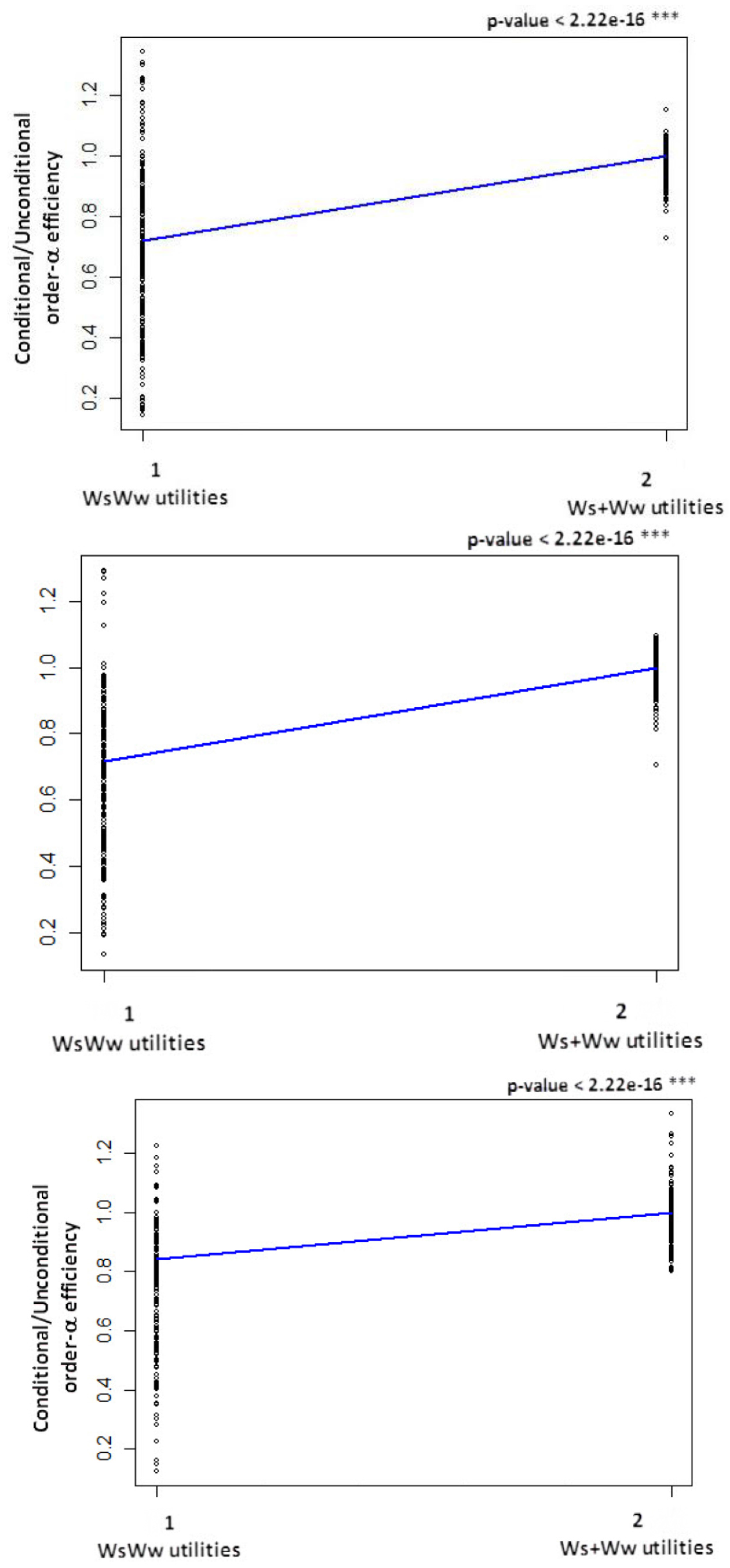
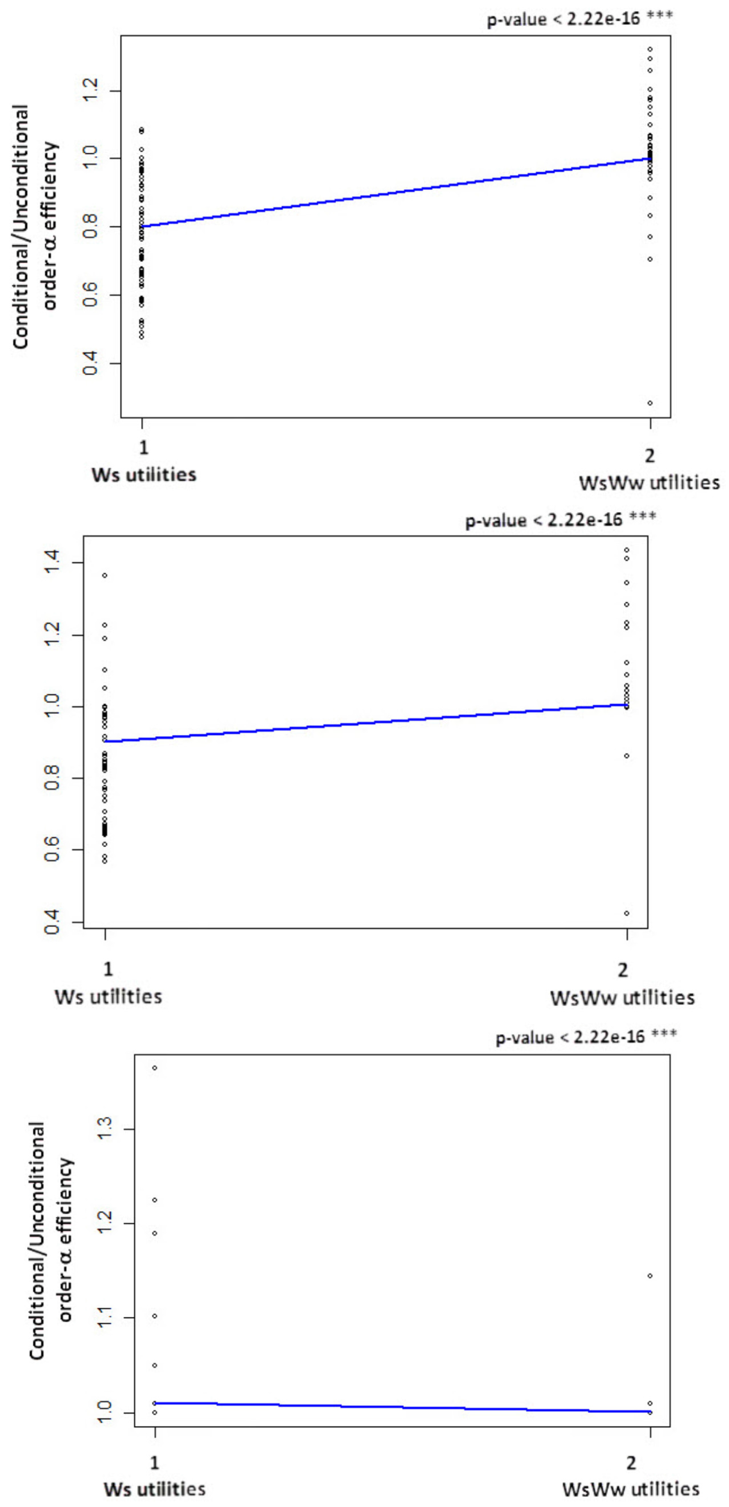
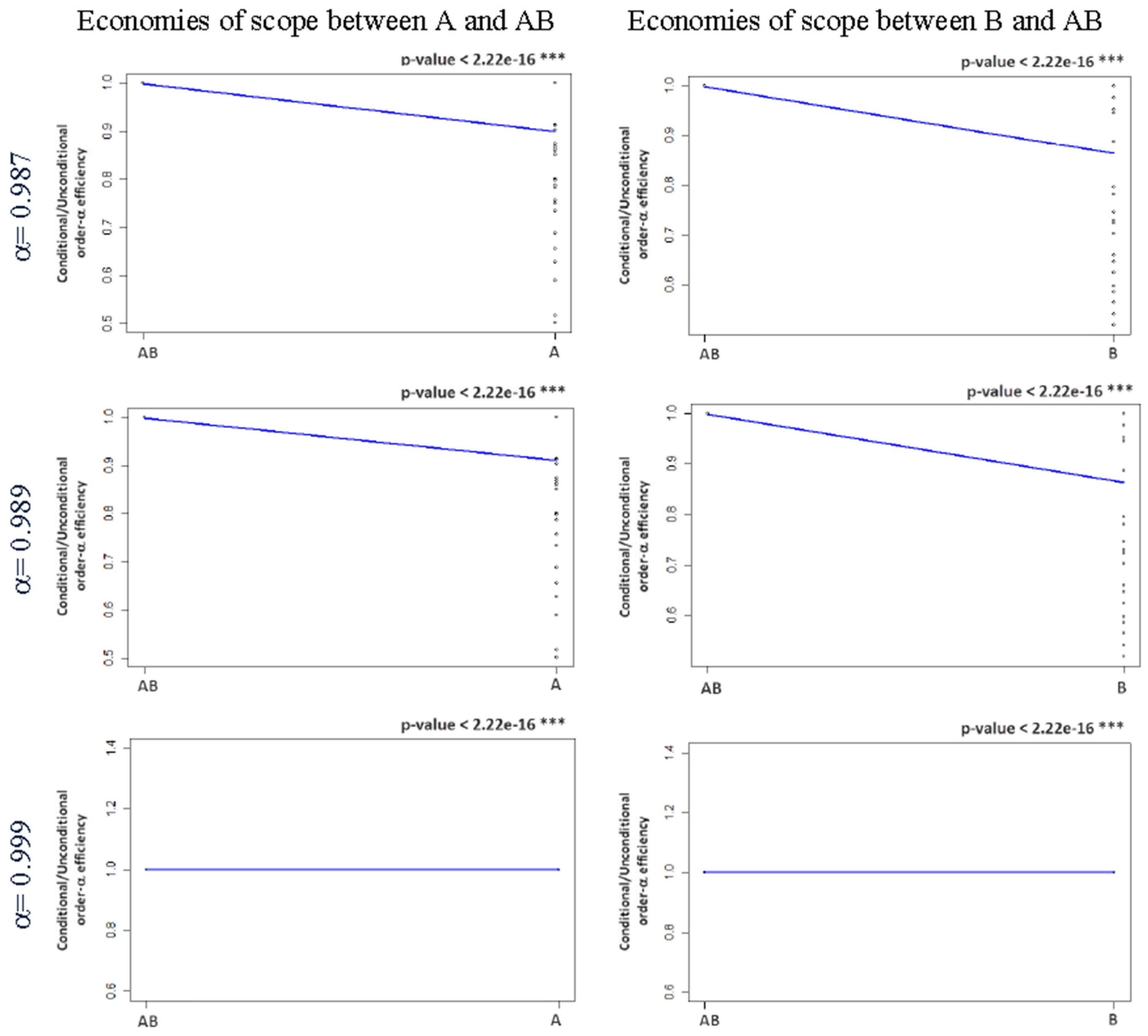
3.3.2. Conditional and Unconditional Efficiency Scores

To test for economies of scope among Ws and WsWw utilities in the Portuguese water sector, we carried out two analyses. First, we analyzed the influence of the exogenous variable “type of utility” on the production process considering the previous two groups of utilities, the group of multiproduct utilities (WsWw) to which corresponds the categorical variable with value 1, and a group of fictitious utilities (separate firms) (Ws+Ww) to which corresponds the categorical variable with value 2. In a second analysis, we examined the influence of the exogenous variable (“type” of utility) just for the real utilities (Ws and WsWw utilities). We considered a categorical variable with values: 1 for Ws utilities and 2 for WsWw utilities. To perform this last analysis it was necessary to build the following two compound outputs which gather outputs from each of the activities provided: “Delivered water volume (retail and wholesale) + 1/3 volume of collected wastewater + 2/3 volume of treated wastewater” (these ratios were assumed since in Portugal the wastewater treatment activity is roughly a weight cost twice the activity of wastewater collection) and “Water customers + Wastewater customers”.

According to the results presented in Figure 9 and Figure 10, the simultaneous provision of water and wastewater services is favorable to performance (at the 99% confidence level), displaying the existence of economies of scope between these activities. When studying the influence of the exogenous variable “type of utility” on the production process of the WsWw multiproduct utilities (1) and the group of fictitious utilities (separate utilities) (Ws+Ww) (2), the existence of economies of scope is clearer. The presence of economies of scope becomes more pronounced (steeper nonparametric regressions) as we move away from a unit value for α. This was also observed in the second analysis when the influence of the exogenous variable on the production process of the real utilities, Ws utilities (1) and WsWw utilities (2) were investigated. However, this second analysis leads to opposite conclusions for higher values of α or, in other words, when it coincides with the full FDH frontier. This may be directly related to the fact that two different types of utilities are compared in this second analysis, particularly a group of multiproduct utilities (WsWw) with a group of utilities that provide only one service (water supply) and that can, therefore, be responsible for skewing the results. This means that this analysis may not be the most appropriate one to find economies of scope, because it compares two completely different types of utilities, some utilities are characterized by an output while others are characterized by two outputs.

Regarding the simulated case study, the application of this methodology has also concluded that utilities A and B are more efficient than utilities AB (Figure 11) and, therefore, diseconomies of scope dominate. However, this finding is extracted from the frontiers $\alpha \le 0.989$, as it is not possible to draw any conclusions from the frontiers near of full frontier ($\alpha \cong 1$) about the existence or absence of economies of scope, since the nonparametric regression is horizontal. This fact highlights the great usefulness of partial frontiers in the search for economies of scope.

The use of this methodology to look for economies of scope needs to be done with care. See, for example, the above analysis in which economies of scope are investigated between utilities A and AB. In the computation of order-α efficiencies, the utilities A can be considered less efficient than utilities AB because they have zero output from output B. To overcome this drawback, we investigated economies of scope using this methodology among the groups of utilities AB and A+B. However, the results do not allow us to prove clearly the existence of scope diseconomies. Only for $\alpha =0.999$ case (frontier near the full frontier) is it possible to conclude that there are scope diseconomies but it is still difficult to prove the existence of diseconomies, given the low slope of the non-parametric regression (Figure 12).

4. Discussion

The results obtained are very encouraging demonstrating the potential of the proposed methodology compared with the other methodologies usually applied in the literature of nonparametric methods. Although the second methodology (which allows the analysis of the influence of the exogenous variables on the production process) is not the most appropriate one to investigate economies of scope, it has also been used in the literature to explore such economies [40]. We argue that the methodology proposed is the most useful since it enjoys all the advantages of the recent partial frontier nonparametric methods. It is a robust tool to investigate economies of scope because it allows us to assess the influence of extreme observations and outliers on the results and does not face the problem of the “curse of dimensionality”, especially when α is farthest from the unit. In addition, our methodology is closer to the definition of economies of scope because it compares the production function of firms that produce two or more goods with the production function of firms that produce only one good. Moreover, not only does it provide an overview of the whole sample but it also enables the evaluation of each observation, and allows us to further assess the robustness of the results obtained by varying the value of α. The results obtained in the simulated case study proves the usefulness and potentiality of the methodology. These results show that if only full-frontier non-parametric methods (such as DEA) were used, we would have concluded quite the opposite. That is, we would have concluded for the predominance of economies of scope when, in fact, diseconomies of scope prevail. The results obtained by the proposed methodology demonstrate that this is caused by 9% of extreme observations, which use a very small amount of inputs and also produce a low level of outputs.

Regarding the case study of the Portuguese water sector, the results obtained by the methodology proposed show the existence of economies of scope between water and wastewater activities in Portugal. These results are in line with most studies in the literature, which find economies of scope between water and wastewater services (e.g., [41,42,43,44]), especially when dealing with small companies. The fact that the water utilities sector in Portugal is characterized by many small water utilities which are vertically unbundled (not integrated) in the retail segment might be one of the main justifications for the existence of economies of scope. The management model of the water utilities in the retail segment in Portugal, contrary to most countries around the world, follows a model which is vertically unbundled (not integrated); that is, in most cases there are different actors supplying the “wholesale” segment (which includes intake, treatment, and transportation in water supply, and transportation and wastewater treatment in the wastewater activity) and the “retail” segment (which includes water distribution in water supply and wastewater collection in the wastewater activity). This last fact may also be one more justification for the existence of economies of scope. Thus, the joint provision of water supply and wastewater collection services may provide a cost advantage, especially in the sharing and joint utilization of resources (inputs), such as human resources (management, administrative labor, and so on), machinery, and information technology, the sharing of technical knowledge, and better coordination of management and maintenance of both networks (which are sometimes interconnected), as well as savings in fixed costs of production, such as purchasing and marketing [45].

5. Conclusions

This paper investigates the use of nonparametric methodologies to estimate the existence of economies of scope, proposing a methodology based on partial frontier methods. These methods are more robust than the full frontier methods, mainly because the partial frontier methods are less sensitive to extreme data and outliers and do not face the problem of the “curse of dimensionality”.

The results of this research show that our methodology to investigate economies of scope is more robust than the ones that use full frontier methods. Firstly, it is closest to the true concept of economies of scope and, secondly, it uses the most robust nonparametric methods, also allowing us to assess the robustness of the results obtained by varying the value of α. In addition, this methodology allows us to evaluate the existence of economies of scope individually for each observation.

Concerning the Portuguese water utilities case study, we found the existence of economies of scope among water utilities and water and wastewater utilities, proving that there could be cost reductions by fostering synergies in providing these two services simultaneously in Portugal. For example, for the order-α quantile frontier of the separate utilities (α = 0.999) and for the order-α quantile frontier of the group of joint production utilities (α = 0.995), on average, WsWw utilities must reduce their inputs in only about 2.8% to become as efficient as separate utilities, while to reach their own frontier they will have to reduce their inputs in about 17.0%.

Therefore, this paper provided evidence of the existence of economies of scope in the water sector in Portugal. Among other reasons, this can be very helpful for decision-makers to reform the water sector since the market structure in Portugal is considered very inefficient. In a period when it is very important, and even compulsory, to recover all the costs by the water utilities, it is socially and politically key to mitigate the impact of tariff increases and market structure reform can be a good contributor for this.

Thus, the policy implications of this investigation refer to the need of Portuguese policy-makers to promote the merger between the wholesale and the retail utilities, the provision, whenever possible, of water and wastewater together and encourage small utilities, for example, with less than 50,000 inhabitants, to provide other services besides water supply and wastewater collection and treatment, such as solid waste, street cleaning, transportation, and gardening, among others.

References

1. Bel, G.; Warner, M. Does privatization of solid waste and water services reduce costs? A review of empirical studies. Resources. Conserv. Recycl. 2008, 52, 1337–1348. [Google Scholar] [CrossRef]
2. Baumol, W.; Panzar, J.; Willig, R. Contestable Markets and the Theory of Industry Structure; Harcourt Brace Jovanovich: New York, NY, USA, 1988. [Google Scholar]
3. Panzar, J.; Willig, R. The economy of scope. Am. Econ. Rev. 1981, 71, 268–272. [Google Scholar]
4. Fraquelli, G.; Piacenza, M.; Vannoni, D. Scope and scale economies in multi-utilities: Evidence from gas, water and electricity combinations. Appl. Econ. 2004, 36, 2045–2057. [Google Scholar] [CrossRef]
5. Abbott, M.; Cohen, B. Productivity and efficiency in the water industry. Util. Policy 2009, 17, 233–244. [Google Scholar] [CrossRef]
6. Farsi, M.; Filippini, M. An analysis of cost efficiency in Swiss multi-utilities. Energy Econ. 2009, 31, 306–315. [Google Scholar] [CrossRef]
7. Färe, R. Addition and efficiency. Q. J. Econ. 1986, 51, 861–865. [Google Scholar] [CrossRef]
8. Färe, R.; Grosskopf, S.; Lovell, K. Productions Frontiers; Cambridge University Press: Cambridge, UK, 1994. [Google Scholar]
9. Grosskopf, S.; Yaisawarng, S. Economies of scope in the provision of local public services. Natl. Tax J. 1990, 43, 61–74. [Google Scholar]
10. Ferrier, G.; Grosskopf, S.; Hayes, K.; Yaisawarng, S. Economies of diversification in the banking industry. J. Monet. Econ. 1993, 31, 229–249. [Google Scholar] [CrossRef]
11. Prior, D.; Solà, M. Technical efficiency and economies of diversification in health care. Health Care Manag. Sci. 2000, 3, 299–307. [Google Scholar] [CrossRef] [PubMed]
12. Cummins, J.D.; Weiss, M.; Zi, H. Economies of Scope in Financial Services: A DEA Bootstrapping Analysis of the US Insurance Industry; Working Paper; Wharton Financial Institutions Center: Philadelphia, PA, USA, 2003. [Google Scholar]
13. Growitsch, C.; Wetzel, H. Testing for Economies of Scope in European Railways: An Efficiency Analysis; Working Paper no. 72; University of Lüneburg: Lüneburg, Germany, 2007. [Google Scholar]
14. Arocena, P. Cost and quality gains from diversification and vertical integration in the electricity industry: A DEA Approach. Energy Econ. 2008, 30, 39–58. [Google Scholar] [CrossRef]
15. De Witte, K.; Marques, R. Big and beautiful? On non-parametrically measuring scale economies in non-convex technologies. J. Product. Anal. 2011, 35, 213–226. [Google Scholar] [CrossRef]
16. Simar, L.; Wilson, P. Sensitivity analysis of efficiency scores: How to bootstrap in nonparametric frontier models? Manag. Sci. 1998, 44, 49–61. [Google Scholar] [CrossRef]
17. Dyson, R.G.; Shale, E.A. Data envelopment analysis, operational research and uncertainty. J. Oper. Res. Soc. 2010, 61, 25–34. [Google Scholar] [CrossRef]
18. Fuentes, R.; Torregrosa, T.; Ballenilla, E. Conditional Order-m Efficiency of Wastewater Treatment Plants: The Role of Environmental Factors. Water 2015, 7, 5503–5524. [Google Scholar] [CrossRef]
19. Daraio, C.; Simar, L. Advanced Robust and Nonparametric Methods in Efficiency Analysis. Methodology and Applications; Springer: New York, NY, USA, 2007. [Google Scholar]
20. Charnes, A.; Cooper, W.; Rhodes, E. Measuring the efficiency of decision making units. Eur. J. Oper. Res. 1978, 2, 429–444. [Google Scholar] [CrossRef]
21. Deprins, D.; Simar, L.; Tulkens, H. Measuring labor efficiency in post offices. In The Performance of Public Enterprises: Concepts and Measurements (pp. 243–268); Marchand, M., Pestieau, P., Tulkens, H., Eds.; North-Holland Publishing Company: Amsterdam, The Netherlands, 1984. [Google Scholar]
22. Daraio, C.; Simar, L. Introducing environmental variables in nonparametric frontier models: A probabilistic approach. J. Product. Anal. 2005, 24, 93–121. [Google Scholar] [CrossRef]
23. Carvalho, P.; Marques, R. The influence of the operational environment on the efficiency of water utilities. J. Environ. Manag. 2011, 92, 2698–2707. [Google Scholar] [CrossRef] [PubMed]
24. Fried, H.; Lovell, K.; Schmidt, S. The Measurement of Productive Efficiency and Productivity Growth; Oxford University Press: New York, NY, USA, 2008. [Google Scholar]
25. Cazals, C.; Florens, J.; Simar, L. Nonparametric frontier estimation: A robust approach. J. Econom. 2002, 106, 1–25. [Google Scholar] [CrossRef]
26. Aragon, Y.; Daouia, A.; Thomas-Agnan, C. Nonparametric frontier estimation: A conditional quantile-based approach. Econom. Theory 2005, 21, 358–389. [Google Scholar] [CrossRef]
27. Daouia, A.; Simar, L. Nonparametric efficiency analysis: A multivariate conditional quantile approach. J. Econom. 2007, 140, 375–400. [Google Scholar] [CrossRef]
28. Morita, H. Analysis of economies of scope by data envelopment analysis: Comparison of efficient frontiers. Int. Trans. Oper. Res. 2003, 10, 393–402. [Google Scholar] [CrossRef]
29. Carvalho, P.; Marques, R. Computing economies of vertical integration, economies of scope and economies of scale using partial frontier nonparametric methods. Eur. J. Oper. Res. 2014, 234, 292–307. [Google Scholar] [CrossRef]
30. Chavas, J.P.; Kim, K. Economies of diversification: A generalization and decomposition of economies of scope. Int. J. Prod. Econ. 2010, 126, 229–235. [Google Scholar] [CrossRef]
31. Zhu, J. Quantitative Models for Performance Evaluation and Benchmarking; Kluwer Academic Publishers: Norwell, MA, USA, 2003. [Google Scholar]
32. Chen, Y. Measuring super-efficiency in DEA in the presence of infeasibility. Eur. J. Oper. Res. 2005, 161, 545–551. [Google Scholar] [CrossRef]
33. Aitchison, J.; Aitken, C. Multivariate binary discrimination by Kernel Method. Biometrika 1976, 63, 413–420. [Google Scholar] [CrossRef]
34. Marques, R. Regulation of Water and Wastewater Services: An International Comparison; IWA Publishing: London, UK, 2010. [Google Scholar]
35. Berg, S.; Marques, R. Quantitative studies of water and sanitation utilities: A benchmarking literature survey. Water Policy 2011, 13, 591–606. [Google Scholar] [CrossRef] [Green Version]
36. Ferro, G.; Lentini, E.; Mercadier, A. Economías de Escala en Agua y Saneamiento: Examen de la Literatura; Working Papers hal-00460661; HAL: Villeurbanne, France, 2010. [Google Scholar]
37. Cruz, N.F.; Carvalho, P.; Marques, R. Disentangling the cost efficiency of jointly provided water and wastewater services. Util. Policy 2013, 24, 70–77. [Google Scholar] [CrossRef]
38. Beasley, J.E. Determining teaching and research efficiencies. J. Oper. Res. Soc. 1995, 46, 441–452. [Google Scholar] [CrossRef]
39. Chen, Y.; Du, J.; Sherman, H.D.; Zhu, J. DEA model with shared resources and efficiency decomposition. Eur. J. Oper. Res. 2010, 207, 339–349. [Google Scholar] [CrossRef]
40. Marques, R.; De Witte, K. Is big better? On scale and economies of scope in the Portuguese water sector. Econ. Model. 2011, 28, 1009–1016. [Google Scholar] [CrossRef]
41. Fraquelli, G.; Moiso, V. Cost Efficiency and Economies of Scale in the Italian Water Industry; Working Paper; Hermes Press: Pavia, Italy, 2005. [Google Scholar]
42. Lynk, E.L. Privatisation, joint production and the comparative efficiencies of private and public ownership: The UK water industry case. Fisc. Stud. 1993, 14, 98–116. [Google Scholar] [CrossRef]
43. Hunt, L.; Lynk, E. Privatization and efficiency in the UK water industry: An empirical analysis. Oxf. Bull. Econ. Stat. 1995, 57, 371–388. [Google Scholar] [CrossRef]
44. Martins, R.; Fortunato, A.; Coelho, F. Cost Structure of the Portuguese Water Industry: A Cubic Cost Function Application; Working Paper, No. 9; University of Coimbra: Coimbra, Portugal, 2006. [Google Scholar]
45. Worthington, A.C. Productivity, Efficiency and Technological Progress in Australia’s Urban Water Utilities; Waterlines Report; National Water Commission: Canberra, Australia, 2011. [Google Scholar]
Figure 1. Example of a partial frontier (order-α) (blue) and of a full DEA frontier (orange).
Water 08 00082 g001
Figure 2. Separate production frontiers (SWs+Ww) and joint production frontiers (SWsWw).
Water 08 00082 g002
Figure 3. Separate production frontiers (SWs+Ww) and joint production frontiers (SWsWw) in the output-output space.
Water 08 00082 g003
Figure 4. Example of order-α joint production and separate production frontiers.
Water 08 00082 g004
Figure 5. Linearized frontiers of joint and separate production.
Water 08 00082 g005
Figure 6. Distribution of observations according to the types of services provided for the period 2002–2008.
Water 08 00082 g006
Figure 7. Percentage of observations with economies and diseconomies of scope, considering CRS (a) and VRS (b) technologies.
Water 08 00082 g007
Figure 8. Ratios η ^ as a function of the output YA for various partial frontiers of utilities AB, for CRS (a) and VRS (b) technologies.
Water 08 00082 g008aWater 08 00082 g008b
Figure 9. Nonparametric regressions estimated to investigate the influence of the exogenous variable “type of utility” on the production process of the WsWw multiproduct utilities (1) and the group of fictitious utilities (separate utilities) (Ws+Ww) (2) for various values α considered (α = 0.99, α = 0.995, and α = 0.999) (kernel regression significance test: *** 0.001, ** 0.01, and * 0.05).
Water 08 00082 g009
Figure 10. Nonparametric regressions estimated to investigate the influence of the exogenous variable “type of utility” on the production process of the Ws utilities (1) and WsWw utilities (2) for various values α considered (α = 0.99, α = 0.995, and α = 0.999) (kernel regression significance test: *** 0.001, ** 0.01, and * 0.05).
Water 08 00082 g010
Figure 11. Nonparametric regressions estimated to investigate economies of scope between A and AB and between B and AB for frontiers α = 0.987, α = 0.989, and α = 0.999 of utilities AB and for frontiers α = 0.999 of utilities A+B. Kernel regression significance test: *** 0.001, ** 0.01, and * 0.05.
Water 08 00082 g011
Figure 12. Nonparametric regressions estimated to investigate economies of scope between AB and A+B for frontiers α = 0.987, α = 0.989, and α = 0.999 of utilities AB and for frontiers α = 0.999 of utilities A+B. Kernel regression significance test: *** 0.001, ** 0.01, and * 0.05).
Water 08 00082 g012