Abstract
An unsteady fully three-dimensional model of Lake Binaba (a shallow small reservoir) in semi-arid Upper East Region of Ghana has been developed to simulate its temperature dynamics. The model developed is built on the Reynolds Averaged Navier–Stokes (RANS) equations, utilizing the Boussinesq approach. As the results of the model are significantly affected by the physical conditions on the boundaries, allocating appropriate boundary conditions, particularly over a water surface, is essential in simulating the lake’s thermal structure. The thermal effects of incoming short-wave radiation implemented as a heat source term in the temperature equation, while the heat fluxes at the free water surface, which depend on wind speed, air temperature, and atmospheric stability conditions are considered as temperature boundary condition. The model equations were solved using OpenFOAM CFD toolbox. As the flow is completely turbulent, which is affected by the complex boundary conditions, a new heat transfer solver and turbulence model were developed to investigate the spatial and temporal distribution of temperature in small and shallow inland water bodies using improved time-dependent boundary conditions. The computed temperature values were compared with four days of observed field data. Simulated and observed temperature profiles show reasonable agreement where the root mean square error (RMSE) over the simulation period ranges from 0.11 to 0.44 °C in temporal temperature profiles with an average value of 0.33 °C. Results indicate that the model is able to simulate the flow variables and the temperature distribution in small inland water bodies with complex bathymetry.
Keywords:
small water body; heat transfer; semi-arid region; temperature dynamics; turbulence; RANS; OpenFOAM 1. Introduction
Inland water bodies such as reservoirs and lakes are very important parts of the continental land surface [1]. Reservoirs are typically built to store water for water supply, hydropower or flood control [2]. Knowledge of the mixing characteristics and temperature profile of a lake are important for its operation and management [3]. The thermal structure of water bodies, temperature stratification dynamics and changes in temperature values have a direct impact on the heat storage of lakes and their water quality [4,5,6]. Understanding the heat budget of lakes and reservoirs is crucial for estimating evaporation in the energy budget methods that are widely used [7,8,9,10]. However, measurements of heat exchange between the water surface and atmosphere are scarce. In most cases carrying out measurements for shallow and small inland water bodies is difficult and expensive and needs high level of expertise to obtain reliable measurements over the water surface even for measuring conventional meteorological parameters such as air temperature, wind velocity and so on. Although experimental temperature profiles in lakes are commonly available, the vertical resolutions are often not sufficient for assessing small-scale turbulence effects or investigating variations of water temperature induced by radiative forcing, air temperature as well as wind velocity in shallow waters [7]. As small shallow lakes and reservoirs respond to atmospheric conditions very quickly, precise estimation of the heat transfer between the atmosphere and their surface is extremely important to model the temperature dynamics and stratification in these water bodies [11]. In these water bodies, the near-surface water temperature commonly follows the radiative forcing (solar radiation) trend with an increase during the day and a decrease during the night. The gradient temperature can transport vertically into the water column by (effective) thermal diffusivity, which can be enhanced by the atmospheric parameters, water surface waves and the dynamics of the flow in the water body. Eddy diffusivity and thermal conductivity are important parameters in simulating the diurnal evolution of the temperature in the water bodies. Wind over the water surface affects lake currents, sensible and latent heat fluxes and turbulence as well as surface waves. The time-dependent effects of wind shear stress over the surface can change the flow pattern and thermodynamics of the lake. Therefore, considering the effects of heat transfer and wind-induced flow in small water bodies is so complicated and needs the use of high-resolution simulation to determine the flow parameters.
In the case of shallow and small inland water bodies, which have been used in this study, simulating the flow field requires an additional degree of complexity beyond simulation of a deep and large water body. Including the effects of the time-varying driving forces such as short-wave radiation, air temperature, wind speed and its direction, precipitation, cloud cover, water surface temperature, and variation in water composition (such as salinity and density) in a shallow water body simulation is difficult. In addition, implementing an appropriate approach to compute the heat fluxes through the water surface, the evaporative flux and the source heat due to the penetration of the incident short-wave radiation, which comes with a high degree of uncertainty, needs to be handled carefully. As these complexities introduce approximations and consequently modeling errors, developing a model which be able to simulate the flow variation in a small water body considering the aforementioned uncertainties is very promising. In this paper, we have developed a fully three-dimensional and unsteady hydrothermal model that is capable of simulating the effects of wind and atmospheric conditions over a complex bathymetry to predict the circulation patterns as well as the temperature distribution in the water body. In this model, the atmospheric conditions, with particular attention to heat fluxes over the water surface (sensible and latent heat fluxes), are applied dynamically to reduce the model uncertainties. To verify the capabilities of the model developed in this study, it was applied to a small shallow reservoir in the Upper East Region of Ghana. To evaluate the performance of the model against the observed values of temperature, some quantitative metrics, include root mean square error (RMSE), the mean absolute error (MAE), the relative mean error (RME) and mean error (ME) were applied. From the metrics of model performance evaluation, the results show that the simulated temperature values are in good agreement with the observed values.
2. Water Bodies Modeling
In the last two decades, an increasing interest in predicting the temperature profiles in reservoirs and lakes has been high due to the correlation between temperature, water quantity and water quality [12]. Transport processes in water bodies are inherently three-dimensional, driven by wind, surface thermodynamics, and the topography of the lake. Hence, assessing the water temperature as well as water circulation, inherently requires transport modelling [13]. Mathematical modelling of water temperature in lakes and reservoirs have been carried out over the years to investigate thermal dynamics in water bodies [5,14,15]. However, in many real-world cases, it is not always possible to solve the water temperature equations analytically due to the non-linearity of some parameters at the air–water interface [5,12] even though water temperature has been simulated in these models at various levels of complexity [16].
One-dimensional models (1-D) are extensively applied to estimate vertical temperature profiles in lakes in time. In 1-D models, variations in the lateral directions are assumed to be small with respect to variations in the vertical direction [4]. In terms of a global or regional coupled atmosphere-lake modeling system for water bodies, 1-D models are the best choices since they require low computational resources and are sufficiently fast for long-term simulations [17]. Generally, one-dimensional models are not able to consider horizontal advection terms and this seems to be one of the disadvantages.
In the early 1980s, two-dimensional (2-D) laterally averaged models were used extensively to predict the flow field and temperature distribution in water bodies [16,18,19,20]. Although these 2-D models are computationally efficient and easily implemented, they are not appropriate for simulating flow fields in shallow lakes because these 2-D models are not able to describe the fully three-dimensional flow field in shallow water bodies [12].
Due to the inabilities of 2-D models in capturing mechanisms influencing mixing and temperature dynamics precisely, especially in morphometrically complex lakes and reservoirs, a number of three-dimensional models have recently been presented [11,12,21,22,23,24,25,26]. Flow field prediction and consequently the temperature dynamics determination in water bodies are accomplishable only through fully 3-D models [16]. Liu et al. [21] developed and applied a three-dimensional finite element model to the subtropical alpine Yuan-Yang Lake (YYL) in northeastern region of Taiwan. Leon et al. [27] evaluated the capability of the 3-D model (ELCOM) for coupling it with the Canadian Regional Climate Model (CRCM) on Great Slave Lake, Canada. Politano et al. [16] solved a fully three-dimensional model to predict the temperature distribution at McNary Dam using the commercial code Fluent; and a later study by Wang et al. [28] developed a 3-D numerical model extending the approach of Politano et al. [16] using the open-source code OpenFOAM.
While numerous 3-D models have been described to characterize thermal dynamics in lakes, they have usually been utilized for large and deep lakes where the representation of the boundary geometry is less important than for shallow small lakes [3]. Only a limited number of CFD simulations for temperature distribution in shallow and small inland water bodies can be found [29].
3. Description of Study Site and Data Collection
The Upper East Region of Ghana (UER) has more than 160 small and shallow reservoirs which have different surface areas ranging from 1 to 100 hectares [30]. These small reservoirs are operationally efficient with their flexibility, closeness to the point of use, and requirement for few parties for management [31]. The studied lake is a small and shallow reservoir located in this region. Lake Binaba (10°53′20″ N, 00°26′20″ W) is a man-made lake mainly used for irrigation, fishing, livestock watering, construction, domestic uses and recreation. As shown in Figure 1 a natural stream has been dammed, storing and supplying water for all these uses in Binaba, a small town in the sub-humid region of Ghana [32]. The average lake surface area is estimated around 31 ha with an average and maximum depth of 1.1 m and 4.0 m, respectively. To monitor the meteorological parameters, a floating measurement station was installed over the water surface. Measurements taken included atmospheric parameters (air temperature, wind speed at 2.0 m above the water surface, wind direction and relative humidity), incoming short-wave radiation, sensible heat flux using an Eddy Covariance (EC) System and water temperature profile. These parameters were used to validate the model. Atmospheric measurements and a water thermistor string were situated near the dam body, where the lake depth is around 4.0 m. The water temperature profile was measured with an Onset HOBO Tidbit v2 water temperature data logger with nominal accuracy of ±0.21 °C [33] and in the following depths: 0.100, 0.200, 0.500, 1.100, 1.550, 1.850, 2.150, 2.800, and 3.465 m.
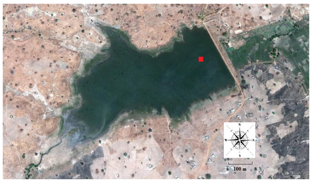
Figure 1.
The shape of Lake Binaba and its surroundings (Google earth). Location of the thermistor chain is shown by a filled square over the lake.
The air temperature fluctuated from 18.0 to 40.0 °C with an average of 28.7 °C while the water surface temperature varied between 24.0 °C and 32.5 °C with an average of 27.5 °C during the measurement period. Measurements were done between 23 November 2012 and 22 December 2012. A four-day period was selected from the observations to simulate the lake temperature and to validate the model as well. Figure 2a shows the diurnal changes of air temperature, with daily variations of approximately 16.0 °C. Incoming short-wave (solar) radiation measurements from the atmosphere to the water surface are shown in Figure 2b. The daily maximum value was recorded around 1:00 p.m. with a value above 800 Wm−2 for most of days. The measured values of relative humidity (RH) over the water surface are shown in Figure 2c. The wind speed and directions, are shown in Figure 2d with south-western direction being the most dominant direction with a maximum speed of 4.0 m/s. Since the wind speed values have been averaged over 30-min intervals (as for the other parameters), instantaneous wind speed may be larger. The variation of atmospheric pressure during the study period was very small and could be ignored. Therefore, the pressure was taken to be a constant 102 kPa for all of the simulations.
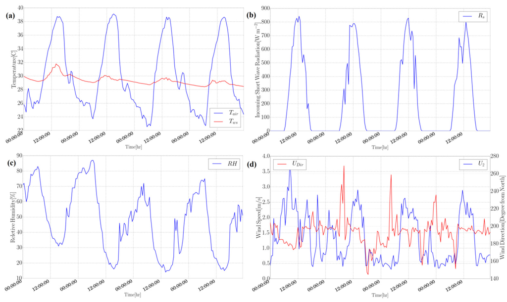
Figure 2.
Measured meteorological parameters used in the simulation: (a) air and water surface temperature; (b) short-wave radiation; (c) relative humidity; and (d) wind speed and its direction.
4. Mathematical Model
4.1. Governing Equations
The flow field was solved with the incompressible RANS (Reynolds Averaged Navier–Stokes) equations. The water can be assumed to be incompressible [34], and the constant-density continuity equation can be written as:
The constant-density (except in the gravity term) momentum equations, using the Boussinesq approach, can be written as:
where is the velocity component in direction (m/s); is time (sec); pressure (Pa); temperature (K); the gravity acceleration vector (m/s2); is the effective kinematic viscosity (m2/s), with and denoting molecular and turbulent viscosity, respectively; the coefficient of expansion with temperature of the fluid (for water ≈ 0.207 × 10⁻³ J·kg−1·K−1); reference temperature (= 293.15 K); and is the delta of Kronecker (dimensionless). The Boussinesq approximation is valid under the assumption that density differences are sufficiently small to be neglected, except where they appear in the term multiplied by [35]. In the model, for incompressible flows the density is considered as effective (driving) kinematic density and calculated as a linear function of temperature as
and the density is calculated from
where (dimensionless) is the effective (driving) kinematic density and water density at reference temperature (≈ 998.24 kg·m−3).
The temperature (instantaneous internal energy) in the water body is computed from the energy conservation equation applicable for incompressible flows as [36,37]:
where is temperature in water (K), heat transfer conductivity (m2/s) and is the heat source term in lake due to the penetrating solar radiation (K/s). Heat transfer conductivity can be given by:
where is the molecular kinematic viscosity (for water at reference temperature ≈ 1.004 × 10⁻⁶ m2s−1), turbulent kinematic viscosity (m2/s), specific heat of water (≈ 4.1818 × 10³ J·kg−1·K−1), is Prandtl number (≈ 7.07), turbulent prandtl number (≈ 0.85) and is effective thermal conductivity (m2/s). Changes in temperature in water body might occur mainly due to heat exchange across the air–water interface. Accurate estimation of heat fluxes is extremely crucial in the simulation of temperature dynamics in the water body [16]. Atmospheric heat fluxes include incoming short-wave (solar) and long-wave (atmosphere) radiations, outgoing long-wave radiation, conductive heat at the free surface and evaporative heat flux. Computationally, all these terms, except for incoming short-wave radiation, are considered at the water surface as boundary conditions.
Incoming short-wave radiation is included in the source term () that allows radiation to be absorbed through a finite distance in the upper layers of the model water column rather than only at the air–water interface [38]. The heat source term using Lambert–Beer law is written as:
where is downward vertical distance from the water surface (m), is the heat flux due to penetrated solar radiation at a depth z* within the water (W/m2), is the net solar radiation at the air–water interface (W/m2), is the fraction of energy contained in the ith bandwidth (dimensionless), and represents the composite attenuation coefficient of the ith bandwidth (m−1) [39,40]. The values of and are presented in Table 1. The attenuation coefficient (light extinction coefficient) for visible light theoretically is a function of wave length, temperature and water turbidity [16,41] and typically ranges from 0.02 to 31.6 for inland shallow waters [16,41,42,43,44]. Usually a linear relationship is applied to calculate the extinction coefficient value from observed Secchi depth in inland water bodies [16,45]. For this study, the attenuation coefficient is assumed to be constant in the whole water body ( m−1). This value was computed from the turbidity measurements. By applying the approach proposed by Williams et al. (1981) [46] and using the available measurements for Secchi depth values during the simulated period, the attenuation coefficient was calculated. The attenuation coefficient value was estimated only in one point and therefore, it is assumed that the distribution of the attenuation coefficient in the water body is homogeneous. The temperature profiles in a shallow lake are significantly sensitive to the attenuation coefficient and, hence, this parameter should be considered carefully in the simulation [29].

Table 1.
Short-wave radiation bandwidth fractions of the total energy () and composite attenuation coefficients () (adopted from [39]).
The net solar radiation at the air–water interface () is given by [47]:
where is the incoming short-wave radiation at the water surface (W/m2) and is the reflection coefficient of solar radiation from water surface (≈ 0.08) [48].
4.2. Turbulence Modelling
In this study, the turbulence is modeled with the realizable (RKE) model. The results of the study done by Shih et al. [49] has shown that the realizable model performs better than the standard (SKE) model or other traditional models. In simulating flow field alongside heat transfer in the water body, it was found that the realizable model is robust with reasonable accuracy and provides better results than the standard or other traditional models [49,50,51]. In this turbulence model, the Reynolds stresses are limited by physical-based mathematical constraints [52]. In the SKE model, dissipation rate for fluctuation is approximated by the dynamic equation vorticity. In addition, the realizable is expected to enhance the numerical stability in turbulent flow simulations. In this model, the turbulent kinetic energy ( in m2/s2) and the turbulent dissipation rate ( in m2/s3) are obtained from:
where is the turbulent kinematic viscosity (m2/s), are the production of turbulent kinetic energy by the mean velocity gradient (m2/s3), is the production of turbulent kinetic energy by the buoyancy (m2/s3), and (m2/s3) and (m2/s4) are the source terms which include the effects of wind on and equations respectively. The parameter (dimensionless) is not constant and depends on the flow conditions and is a function of the ratio of the velocity components in the vertical and longitudinal directions [53]:
where and are the components of the flow velocity perpendicular and parallel to the gravitational vector respectively (m/s). The coefficient (dimensionless) is evaluated as [49]:
and the turbulent kinematic viscosity is given by
where is the mean rate-of-rotation tensor. and are written as
where (≈ 0.85) is the turbulent Prandtl number for energy [51]. The standard values of the model constants used for the realizable turbulence approach in the model equations are given as [49]:
Depending on the approach used to implement the effects of wind velocity over the water surface, the source/sink terms in Equations (11) and (12) can be parameterized [29]. In this study, the effects of wind velocity is considered as a shear stress boundary condition over the water surface and therefore, the source/sink terms are given by:
5. Numerical Simulation
5.1. Numerical Grid
In order to perform reliable Computational Fluid Dynamics (CFD) computations in complex geometries such as for lakes or reservoirs, the generation of a good computational grid (mesh) is essential. Numerical modeling of shallow water bodies is generally computationally expensive. In such domains the vertical length scale is much smaller than the horizontal scale. As a consequence, the vertical grid aspect ratio to the horizontal directions is small and numerical instability may be introduced. To avoid this instability, a large number of horizontal grid points are required to decrease the maximum aspect ratio of the grids. The extra grids will, however, increase the computational time significantly [53].
Lake Binaba is characterized by significant bottom slopes throughout its area. As the effects of morphometry are significant [54], preparing the precise geometry (bathymetry) was important. Using the proposed approach by Abbasi et al. [29] and the available (rough) bathymetry measurements, the lake geometry was generated (Figure 3a) and used in the snappyHexMesh [55] utility available in OpenFOAM [56] to generate the computational mesh. snappyHexMesh is a powerful script-driven, unstructured mesh generator. This utility generates grids containing hexahedra and split-hexahedra [57,58].
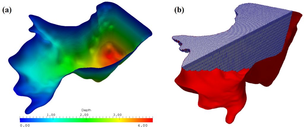
Figure 3.
(a) The generated geometry of Lake Binaba with depth distributions; and (b) computational grid in the water body used in the simulation (vertical exaggerated by 100).
The computational mesh should follow the bathymetry of the lake. Horizontal grids were generated according to the geometrical boundaries. In the vertical direction (), grid spacing was varied so it was concentrated only where the specific resolution was required (Figure 3b). Concentration of the vertical grid points near the boundaries, especially for water surface, was more clustered to cover the sharp gradients in resolved parameters.
The generated computational grid was composed of 41,400 grid points and 35,617 cells. The computational grid for the lake was selected based on coarse and fine meshes to select the optimized number of cells. The selected mesh was refined sufficiently near the water surface to accommodate the high gradients, specifically in velocity and temperature.
5.2. Numerical Setup
The model improvements explained in Section 4, were implemented in OpenFOAM CFD package [56]. OpenFOAM includes a set of efficient C++ modules that could be used to establish solvers. Because of the collocated and polyhedral numerics implemented in OpenFOAM, it can be used in both structured and unstructured meshes with the advantage of being easily extendable to run in parallel. To respect the structure of the original code, a new turbulence model including the buoyancy effect and a new heat transfer solver were implemented. The solver is an unsteady state and incompressible heat transfer solver that considers buoyancy effects in the momentum equation. The PIMPLE method was used for pressure-velocity coupling. The PIMPLE algorithm combines the SIMPLE (semi-implicit method for pressure-linked equations) algorithm and the PISO (pressure implicit with splitting of operators) algorithm to rectify the second pressure correction and correct both velocity and pressure explicitly. This algorithm allows one to use larger time steps than PISO algorithm. Due to the transient conditions of flow in the lake, an adaptive time-stepping technique based on the Courant–Friedrick–Levy number (CFL) was used [59]:
where , and are the velocity components in x-, y- and z-directions, respectively (m/s). In this study, the maximum value of global CFL adopted was 0.2. For larger time steps numerical dissipation increases as the CFL-number increases and makes the model more unstable [36,51].
6. Boundary Conditions
6.1. Temperature
Meteorological and water temperature measurements were available (Figure 2) for the simulation period. At the atmosphere-water surface interface, the temperature gradient evaluated at the lake surface is described by the following equation (Neumann Type) [43]:
The net heat exchange between the water surface and atmosphere () includes four heat flux terms [11,43]:
where is the net long-wave (atmospheric) radiation from atmosphere, is the long-wave (atmospheric) radiation from the water surface, and and are the sensible and latent (evaporative) heat fluxes between the lake surface and atmosphere, respectively. Measurements of heat fluxes such as short-wave radiation, long-wave radiation, sensible heat flux, and latent heat flux are very difficult and expensive to take. Therefore, these heat fluxes are often parameterized using the most commonly available meteorological data [11]. In the current study, the incoming short-wave radiation was the only surface heat transfer term that was directly measured. The rest of the surface terms were computed within the model at each time step using standard formulae. It should be mentioned that in the current model, does not include the short-wave (solar) radiation. This term is included in temperature equations (Equations (5) and (9)) as the source term.
Atmospheric long-wave radiation was calculated from the Stefan–Boltzmann law [11,43]:
where is the reflection coefficient of atmospheric radiation from water surface (≈ 0.03) [60,61], emissivity of atmosphere (≈ 0.87) [62], is Stefan–Boltzmann constant (≈ 5.67 × 10⁻⁸ Wm−2K−1), and is absolute air temperature in K. Similarly, long-wave radiation from the water surface was estimated by [1,11,43]:
where is emissivity of water (≈ 0.97) [14,63], and is the absolute temperature of the water surface in K.
In general, latent heat flux (evaporation) is one of the most important parameters in heat dissipation, but its prediction is the most inaccurate. In most available methods for evaporation estimation, the models’ parameters are specific to a given water body under the prevailing surrounding environment and for a specific climate which are valid only for the specific ranges of parameters (reservoir size, temperature difference, humidity, atmosphere conditions, etc.) that are used in the designed experiment. This therefore means these coefficients may not provide satisfactory estimation for other regions. In this study, for sensible heat () and latent heat () fluxes, the following formulae were used. These equations were obtained from a CFD-based approach (CFD-Evap Model) applied for Lake Binaba [64]. The convective heat transfer between a water surface and the atmospheric boundary layer can be expressed as follows:
where is the convective heat transfer or sensible heat flux in W/m2 (positive if it flows from the atmosphere into the water surface) and is the convective heat transfer coefficient (Wm−2·K−1), which relates the convective heat flux normal to the water surface to the difference between the water surface temperature () and surrounding air temperature (). The convective heat transfer coefficient can be estimated by [64]:
Using the analogy between the heat and mass transfer, the convective mass transfer coefficient was derived as a function of wind velocity. The evaporation rate from the water surface could then be calculated using the estimated mass transfer coefficient:
where the evaporation rate is expressed in Wm−2, and are the water vapor mixing ratio of air and water surface, respectively (kg(water)/kg(dryair)), is the air density, assumed constant in this study ≈ 1.186 kg m−3, the coefficient is used for converting the latent heat flux to mm/day and the coefficient of converts it to W/m2 to be consistent with the rest heat flux components over the water surface, and is the mass transfer coefficient given by [64]:
where is in ms−1 and in ms−1 and the respective constant values in the sensible and latent heat flux equations specific to the studied lake obtained from CFD-Evap model [64], and , were calculated by:
where is atmospheric pressure (= 102 kPa), is the saturation vapor pressure at the temperature of the water surface (hPa) and is the vapor pressure at the air temperature (hPa) given by [65]:
where RH is relative humidity (%) and water surface () and air () temperatures are in °C.
These heat fluxes are defined to be positive if heat flows from the atmosphere into the water surface. Heat fluxes induced by inlets and outlets and precipitation are generally neglected [66].
Determining the correct heat fluxes for a water surface boundary is often difficult. The main difficulty is that is a function of various parameters, where each of them has to be computed by using its own formula and sets of coefficients as well [43]. Therefore estimation of needs a great deal of judgment in adopting the suitable formula, which depends on many uncertain parameters [11]. In addition, some components of the net heat flux depend on unknown water surface temperature values (), which creates an implicit boundary condition that should be calculated in each time step in advance by the model. Although using a heat flux boundary condition over the water surface needs more computational resources, it needs no costly observed water surface temperature. This temperature boundary condition, which includes heat fluxes at the water surface, given by Equations (33) through (37), was implemented in the current model by using the groovyBC [67] library developed for complex boundary conditions.
Another alternative, but less practical, temperature boundary condition on the water surface uses measured water surface temperature values as boundary condition (Dirichlet type) for temperature. Using observed values of water surface temperature as water surface boundary condition has the advantage of avoiding the uncertainties in the net heat flux estimation [43] but the model needs extra measurements over the water surface that is rarely available in most small lakes. The disadvantage of using measured water surface temperature is that using this boundary condition assumes homogeneous temperature at the open water surface which introduces error in the simulation.
In shallow lakes, the temperature boundary condition at the bottom and sides are very complex and need extra measurements to implement in the model. To simulate the effects of bottom and sides, the absorbed and reflected penetrated short-wave radiation should be measured. In addition, the heat flux from these boundaries has to be specified. In spite of the importance of these parameters, measuring their values is not easy and needs extra equipment. Regarding the available measurements, the boundary condition at the bottom of lake and side walls were set to zero heat flux conditions (adiabatic condition) and given by [1]:
where T is temperature in (°K). The measured temperature profile at start time (on 24 November 2012 at 12:00:00 a.m.) was used as the initial condition for temperature for the simulation.
6.2. Velocity
Wind over the water surface affects lake currents, sensible and latent heat fluxes and turbulence, as well as surface waves. The effects of wind shear stress over the flow was considered as a time-dependent shear stress boundary condition over the water surface. The shear stress over the water surface is given by:
where
where is the drag coefficient (unitless), is the air density (kg/m3), and are horizontal shear stress components over the water surface (kg m−1 s−2), and are horizontal components of the mean wind speed over the water surface (m/s), and is the effective kinematic viscosity (m2/s). The empirical dimensionless drag coefficient () depends to large extent only on wind speed and the state of wave development or wave age. For small shallow lakes, wind speed is generally low U10 < 5 ms−1, where U10 is wind speed at height 10 m above the water surface (Figure 2d) and measurements of the drag coefficient are relatively scarce. Confusingly, in the literature, the values of vary over a wide range and it is associated with large scatter [3,43,68]. In this study, the following empirical relationship for low wind speeds measured at a height of 10 m is used [68,69]:
where is the drag coefficient (unitless) and is the wind velocity at height 10 m above the water surface (m/s). In this study, the wind speeds were measured at a height of 2 m from the water surface hence the observed values were converted to its values at 10 m using logarithmic distribution function for wind speed. The normal component of velocity over the water surface boundary was calculated by:
On the other boundaries, the non-slip conditions for velocity and zero heat flux for temperature and the standard wall functions were imposed [16,43].
7. Numerical Results and Discussion
A large number of simulations were run during the model development. The simulation was run for four days (345,600 s) where the starting time of calculations was at 12:00:00 a.m. on 24 November 2012. The simulated flow field in the water body shows the existence of an unsteady and three-dimensional flow for most times due to the effects of the reservoir geometry, dynamic atmospheric conditions and the coupling of energy (temperature) changes with the flow field.
To validate the model, the distribution of simulated temperature in the water body was compared with observations as shown in Figure 4. For each depth where the temporal temperature profile is depicted in Figure 4, the mean error ( where and are measured and simulated temperature values, respectively) or relative mean error () are provided as a measure of the bias of the simulated values. The calculated values of ME and RME for each depth are presented in Table 2. As shown in Table 2, the maximum difference between the simulated and observed values is −1.60 where the minus sign means the model overestimated the temperature. Alongside the ME and RME, the root mean square error () and the mean absolute error () are provided as the measures of the overall goodness-of-fit of the simulations to the observations. The values of RMSE between the simulated and observed values of temporal temperature profiles at different depths range from 0.11 to 0.44 °C with an average value of 0.33 °C. Similarly, the calculated MAE ranges from 0.03 to 0.31 °C with an average of 0.21 °C. As was expected considering the depicted temperature profiles in Figure 4, the RMSE as well as the MAE are increasing in greater depths. A good agreement between simulated and observed temperatures demonstrate the capability of the model to represent temperature dynamics in the small and shallow inland water bodies. These results clearly indicate the variability in the temperature and velocity distributions and the daily thermal cycle predicted by the model for the studied meteorological conditions. Although deviations between modeled and observed temperature profiles at some depths, especially at greater depths were relatively large, general trends and daily temperature fluctuations due to heat transfer are reasonably reproduced by the model. These large deviations between the simulated and observed values are mainly due to the existing uncertainties in thermal boundary condition assigned to the bottom and sides of lake considering the available data or applicable measurements. As shown by Suarez et al. [70], in shallow water bodies the thermal interaction between the reservoir bottom, which includes both the bottom and the sides, and the sediment beneath the reservoir significantly affects the reservoir thermal structure. In addition, ignoring the variations of turbidity in the water column and changes of the extinction coefficient of water in this simulation can be considered as the error sources, especially at greater depths [41,70,71]. To evaluate the effects of upper thermal boundary condition (on the water surface) on the temperature profiles, both boundary conditions for temperature described above were considered. In both simulations, the same differences were found between the simulated and observed temperature values at greater depths.
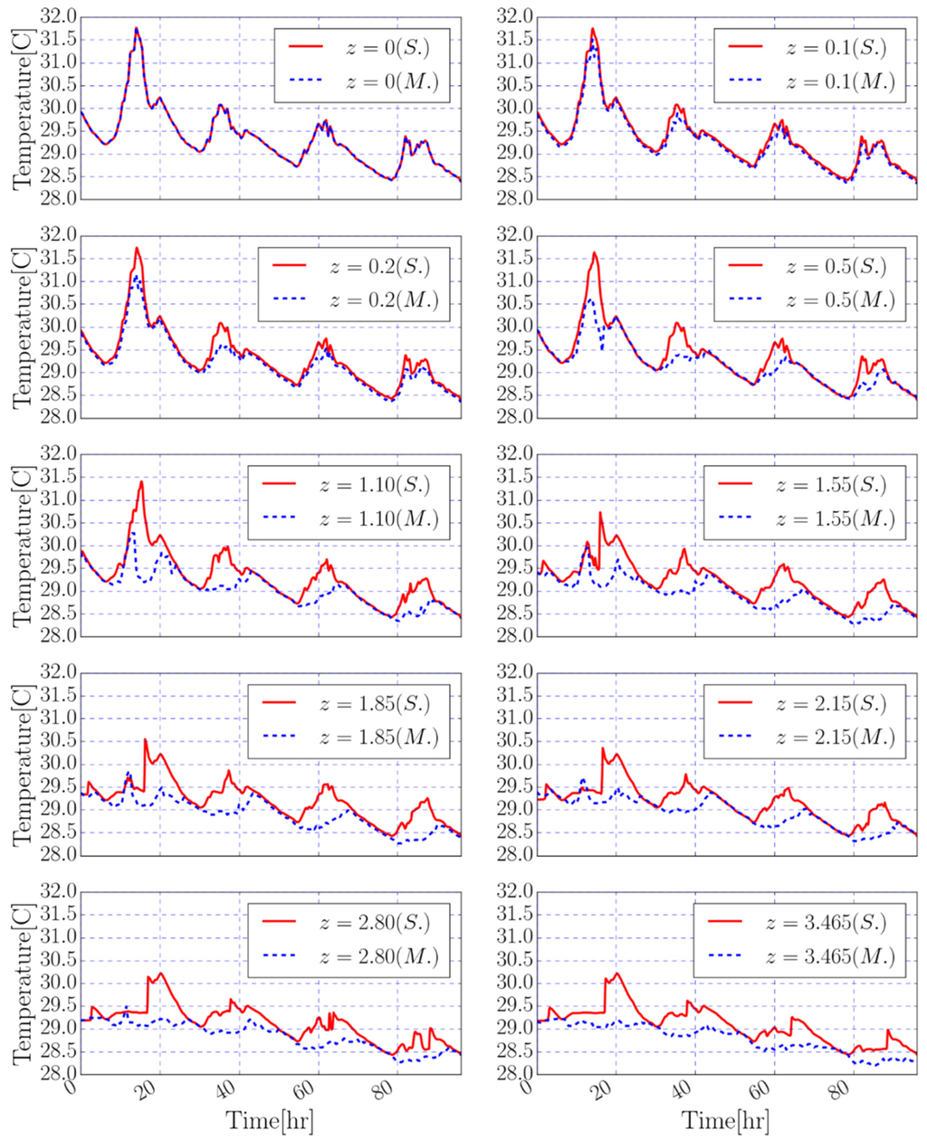
Figure 4.
Simulated water temperature (S.) and observed values (M.) at different depths (at water surface as well as depths of 0.100, 0.200, 0.500, 1.100, 1.550, 1.850, 2.150, 2.800 and 3.465 m).

Table 2.
Calculated metrics of model performance (MAE: mean absolute error; RMSE: root mean square error; ME: mean error; RME: relative mean error) for simulated temporal temperatures at different depths.
In Figure 4, the simulated water temperature (S.) and observed values (M.) at different depths are depicted. These temporal profiles of temperature were generated by using the heat flux as the temperature boundary condition (Section 6.1) on the water surface. These profiles show that in each day of simulation, two different time periods can be detected. In the first time period, which commonly (in the four-day simulated period) ranges from 12:00:00 till 6:00:00 a.m., the simulated temperature matched the observed ones. In this period, due to the good agreement between the modeled and observed temperatures the model can predict the heat budget of the lake precisely. In the second time period, which commonly expands from 6:00:00 a.m. till 12:00:00 a.m., the model overestimated the temperature and consequently the heat content of the lake. As these time periods occur periodically in the simulated period, it seems that the model’s excess heat during the second time period (from 6:00:00 a.m. till 12:00:00 a.m.) is matched by excess cooling at the first period. Therefore, in spite of the uncertainties and errors discussed above, the model could be applied precisely for estimating heat budget of lakes through a one-day time step. This aspect of the model can be promising in energy budget method for evaporation estimation where ignoring the heat content of the lake usually makes significant error in the estimated evaporation from the water surfaces [7,9].
To analyze the simulated temperature profiles with respect to the incoming short-wave radiation, by following the proposed approach by Vercauteren et al. (2011) [7], the amplitude and the phase shift of the observed and the simulated daily temperature variations (24 November 2012) as a function of the depth are plotted in Figure 5. As Figure 5 shows the model overestimated both the amplitude and the phase shift in all depths and the differences between the simulated and measured values are increased with depth. Although the applied model in this study is fully 3-D and considers the horizontal flows, analyzing the amplitude and phase shift of the temperature signals helps to find the order of the importance of radiation as well as the turbulent diffusivity (or heat conductivity) on temperature profiles.
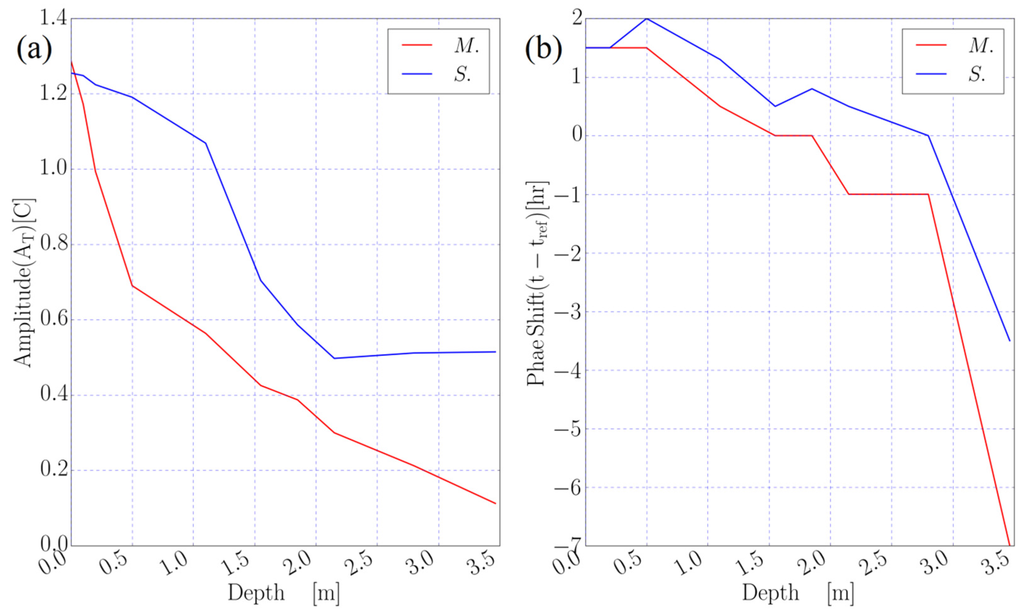
Figure 5.
Analysis of the simulated (S.) and observed (M.) temperature values on the selected day (24 November 2012). (a) Amplitude of the daily temperature variations as a function of depth. Amplitude is defined as the half-temperature fluctuations (the difference between the maximum and minimum temperature values in each depth); (b) The phase shift with respect to the maximum short-wave radiation value as a function of depth where t and tref are the times of the maximum temperature and short-wave radiation respectively.
As on the selected day (24 November 2012), the wind speed was low (Figure 2d), it is expected that incoming short-wave radiation has the dominant effect (in comparison with the turbulent diffusivity) on the temperature profiles. The overestimated amplitude and phase shift of temperature signals show that the model overestimated the radiation effects especially on the calm days and consequently radiation can lead to an overestimation of the turbulent heat transfer conductivity [7]. It can be concluded that the optical properties of the water bodies should be considered carefully in shallow lake models to enable one predict the temperature signals due to the significant effects of radiation on both the amplitude of the temperature oscillations as well as the phase shift.
The vertical simulated temperature distribution through the water body, in seven distinctive time frames were plotted in Figure 6. These time frames were chosen in a way that they cover both the heating and cooling phases in the lake. To show the performance of the model with respect to the vertical temperature profiles, the measured vertical temperature profiles are plotted as well in Figure 6 with dotted lines for the same time frames. At the beginning part of the simulation (from 12:00:00 a.m. to 7:00:00 a.m.) the water surface is cooling and the value of temperature source () is equal to zero. During the cooling time, the wind speed over the water surface is low (less than 1.0 m/s). Looking at the simulated temperature profile, during the cooling phase (at t = 7 h) there are very small differences at different depths and the lake could be considered as a well-mixed water body (Figure 6). This condition could be useful in making some simplifications in calculating the heat budget of the lake to calculate evaporation from the water surface in energy budget methods. As the radiative heating intensifies, the water temperature in the top layers near the water surface increase as a consequence of the penetrating short-wave radiation from the water surface. It should be mentioned that during the heating phase (from 7:00:00 a.m. to 6:00:00 p.m.) the values of over the water surface remains negative. Due to the effects of absorbed radiation, applied as source term in temperature equation, the temperature increases especially in the top layers near the water surface from 7:00:00 a.m. until 2:00:00 p.m. where the incoming short-wave radiation is increasing. As the incoming short-wave radiation decreases on the water surface from 2:00:00 p.m. to 12:00:00 a.m., the temperature decreases in the top layers to reach to the well-mixed condition (at t = 24 h). The behavior of the water body in the heating phase is completely different from the cooling phase. In the heating phase the water body is not well-mixed; hence, to estimate the heat budget applicable in the evaporation calculation, the non-uniform simulated distribution of temperature is used.
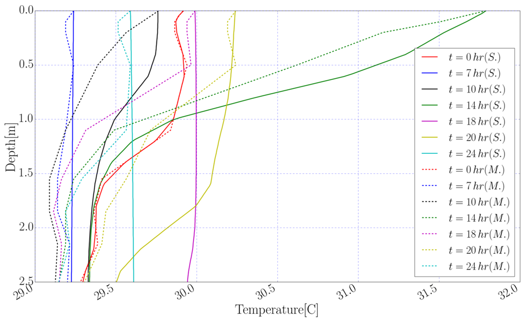
Figure 6.
Simulated vertical temperature profiles (S.) and observed values (M.) at selected time frames.
According to Equation (2) in the governing equations of the model, the flow was coupled with energy in the lake. Therefore, changes in temperature impact the flow field. The velocity distribution at different depths and stream lines in the lake show the transient boundary conditions over the water surface and complex bathymetry of lake which make the flow in the lake unsteady and fully 3-D. Assuming that the top grid cells near the free water surface represent the temperature and velocity at the free surface, the horizontal distributions of velocity field at the water surface are presented in Figure 7.
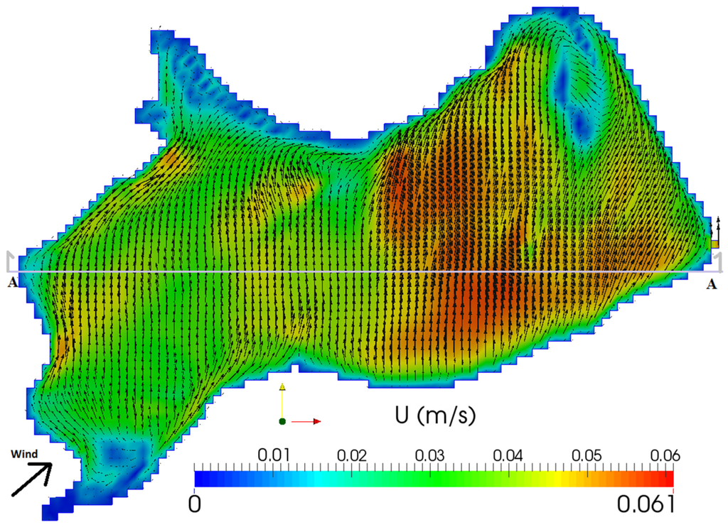
Figure 7.
Simulated velocity vectors and their magnitudes over the water surface at t = 1:00 p.m. where U2 = 1.0 ms−1. Line A-A is the vertical section illustrated in Figure 13.
Figure 7 and Figure 8 present the velocity fields at two different depths, at the water surface and at 1 m beneath the water surface at 1:00 p.m. As expected, there were return currents at this depth. The simulated vertical velocity profiles show non-uniform distributions, where flow near the bottom and sides tend to follow the bathymetry.
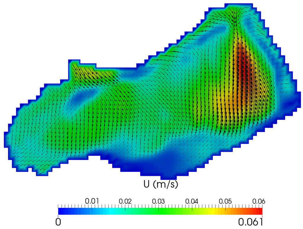
Figure 8.
Simulated velocity vectors and theirs magnitudes at 1 meter beneath the water surface at t = 1:00 p.m. where U2 = 1.0 ms−1.
As shown in Figure 9 and Figure 10, the higher wind speeds caused more mixing in the water column in the vertical direction and consequently lead to higher return flows, which were generated between the surface and deeper layers. Wind induced circulation mainly affects the region near the free water surface and its effects are negligible near the bottom of the lake. In deep regions, this process consequently separates the bottom layer from the top mixed layer and leads to stratification. However, in shallow regions, winds at the water surface can generate circulation throughout the whole depth, from the surface to the bottom of the lake, and therefore in the shallow parts there was no significant stratification most of the time (Figure 13). In general, as can be seen in Figure 8 and Figure 11, the velocity distributions in the horizontal section are greatly dependent on wind speed and its direction at the water surface. Higher wind velocities induce strong horizontal circulation as corroborated by Lee [53].
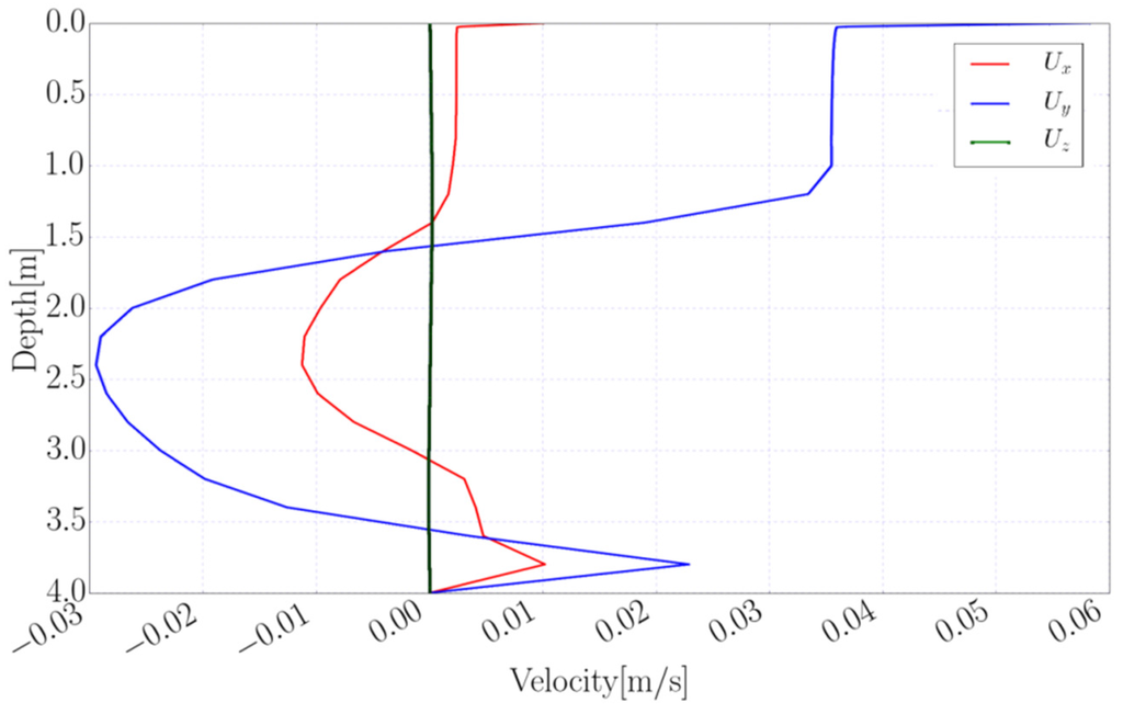
Figure 9.
Simulated vertical distribution of velocity components in the water body where U2 = 3.0 ms−1.
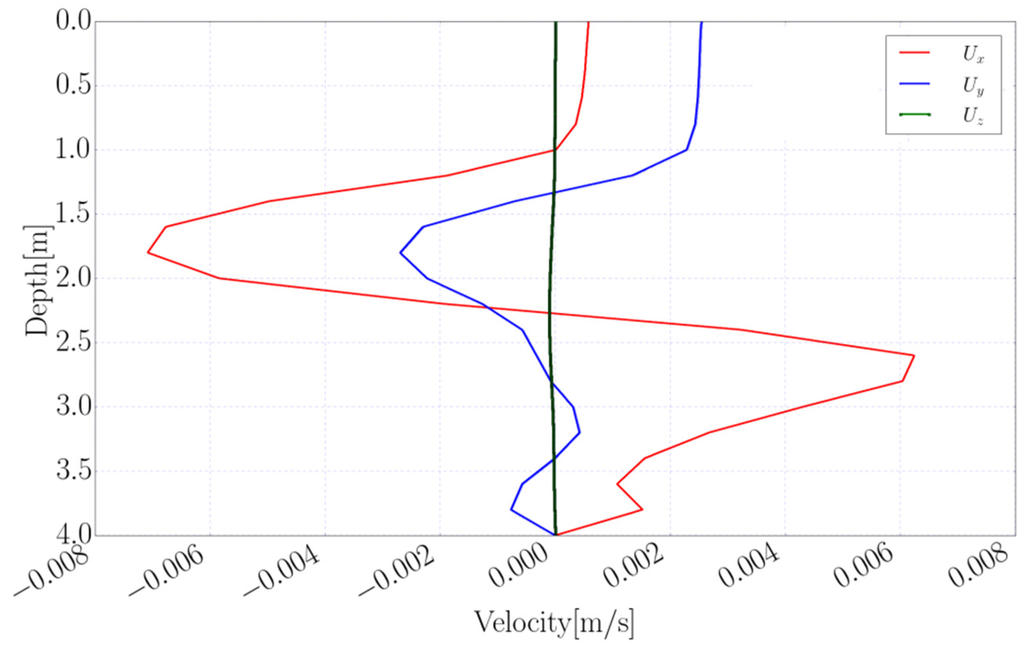
Figure 10.
Simulated vertical distribution of velocity components in the water body where U2 = 0.7 ms−1.
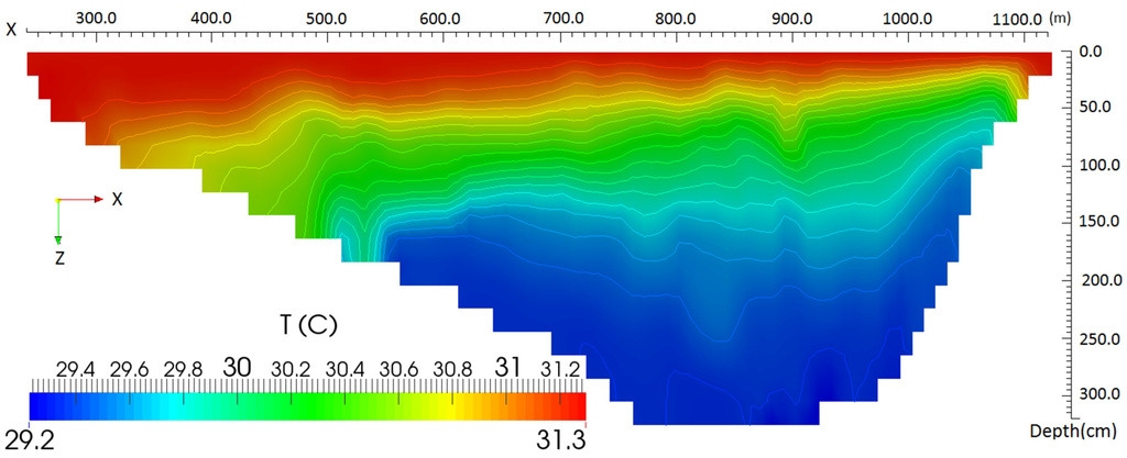
Figure 13.
Simulated Temperature field (values and contours) in a vertical section of the lake shown as line A-A in Figure 7 at t = 1:00 p.m. (vertical exaggerated by 100).
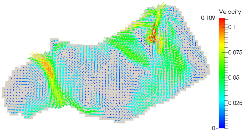
Figure 11.
Simulated velocity field (stream lines) at 1 m beneath the water surface at t = 9:00 a.m. where U2 = 3.8 ms−1.
Figure 12 shows the simulated temperature values in a horizontal section at 1 m beneath the water surface. As can be seen, the temperature distribution is not uniform and the temperature difference between the points at similar depth is around 1.4 °C. The vertical distribution of temperature in a vertical section is illustrated in Figure 13, which shows that the behavior of shallow and deep parts are different, and shallow parts respond faster to air heating. Since surface temperature is a complex function of several parameters, such as wind speed, incoming short-wave (solar) radiation, wind direction, humidity, air temperature, etc., it is difficult to detect a general clear pattern in water temperature. However, generally, the simulated results indicate that heating during the day is normally related to incoming solar radiation, while cooling at night is more complicated and is more a function of wind speed and its direction. Water in the surface layer starts to warm after sunrise as incoming solar radiation increases (around 7:00:00 a.m.), and this increase continues until short-wave radiation reduces (at 3:00 p.m.), after which surface water temperatures reduce gradually.
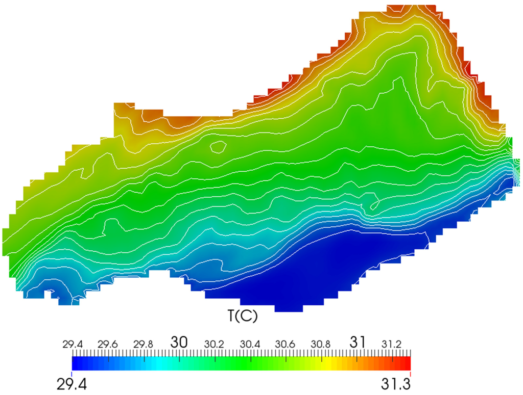
Figure 12.
Simulated Temperature field (values and contours) at 1 m beneath the water surface at t = 1:00 p.m.
Apart from the wind effects on flow field in water bodies, the coupling energy and momentum equations drive the circulation. As solar radiation increases, the temperature in the top layers increases. This increase extends vertically by effective thermal conductivity to the bottom of the lake. With an increase in wind during the day, the velocities at the surface also increases, but no significant vertical circulation is seen throughout the water because of the existence of stable stratification. Water temperature in the top layer is more sensitive to the meteorological conditions. Steeper temperature gradients in the top layers near the water surface are correctly predicted by the model due to the high heat fluxes at the water-air interface.
The main sources of error in the results could be related to the following:
- 1)
- Estimating heat fluxes over the water surface as boundary condition is very uncertain especially for latent heat flux. The location, climate, shape, depth, bathymetry, atmospheric stability conditions, etc. make it difficult to estimate evaporation accurately from the water surface.
- 2)
- There are no measurements for some important parameters that can affect the flow field and temperature in the water body, such as turbidity, and heat fluxes at the bottom and side walls where using simplified temperature boundary conditions could be considered as a source of error.
- 3)
- The measurements were taken only at one point. This means that the distribution of parameters over the water surface was assumed homogeneous. For shallow and small lakes with limited fetch, this assumption could produce a large error in the results.
- 4)
- Coupling the turbulent flow and heat transfer in a shallow water body is complex and computational issues such as numerical errors, mesh dependency and residuals control should be considered.
- 5)
- Errors in field measurements on the water surface especially for water surface temperature or heat fluxes.
Due to the limitation of computational resources, it is not possible to use a finer mesh or very small time steps. In this study different settings for numerical schemes and mesh sizes as well as the time steps were considered to find the optimum situation to make a balance between the needed computational resources and the desired accuracy according to the aims of simulations. For the computational grid used alongside the implemented adaptive time-stepping technique (Section 5.2), different time step values ( seconds) were used in this simulation to prevent numerical stability issues. Four days of simulations, as described in this paper, took about 20 h on the HPC Cloud-based virtual machine with 12 Intel processors at 2.7 GHz and 96 GB RAM [72].
8. Conclusions
The temperature profile in a shallow and small lake in a semi-arid region was simulated. The main aim of the simulation was to find how the flow field and temperature distribution vary spatially and temporally in the shallow inland water body. As the flow in the water body is fully 3-D and turbulent, the full 3-D modified equations of the flow considering the temperature in the water body were solved by a CFD approach using OpenFOAM. The results for Lake Binaba show that the model overestimates the temperature distribution in the water body. This could be related to using boundary conditions with a high degree of uncertainties. The accuracy of the model mainly depends on the error in input meteorological parameters. The profile temperatures and flow pattern in water bodies have been found to have strong correlations with the air temperature, incoming short-wave radiation and wind velocity over the water surface. The effects of other meteorological parameters were considered implicitly in the heat fluxes over the water surface as boundary conditions. One of the big challenges in modeling very shallow lakes is implementing heat fluxes over the water surface accurately especially for the latent heat flux (evaporative heat flux).
According to the results, the lake model could be improved in the following ways: (1) improving the temperature boundary condition on the bottom and sides of the lake by considering heat fluxes through the sediments; (2) improving the methods to estimate heat fluxes over the water surface as temperature boundary condition; (3) considering the effects of the reflected penetrated short-wave radiation in the water body as an extra source term in the lake; and (4) an optimization method to find the optimized number of cells and the regions that should be refined in the lake.
The developed approach could be used for water quality, biological and environmental simulations of shallow water bodies as well.
Acknowledgments
This work was carried out on Dutch national e-infrastructure with the support of SURF Foundation (under grant number e-infra140092). The work was also supported by Challenge Program on Water and Food (CPWF) and the European Space Agency’s TIGER.
Author Contributions
All authors contributed extensively to the work presented in this paper. As specific contributions, Ali Abbasi provided the concept, prepared, designed the model and simulations and wrote the manuscripts; Franke Ohene Annor contributed in providing the data and observations, fieldwork, developing the concept, data analysis and improving the manuscript and figures; and Nick van de Giesen contributed in developing the concept, providing the data and measurements, proofreading the manuscript and verifying the results.
Conflicts of Interest
The authors declare no conflict of interest.
References
- Shufen, S.; Jinfeng, Y.; Nan, X.; Changhai, S. Development of a Model for Water and Heat Exchange Between the Atmosphere and a Water Body. Adv. Atmos. Sci. 2007, 24, 927–938. [Google Scholar]
- Casamitjana, X.; Serra, T.; Colomer, J.; Baserba, C.; Pérez-Losada, J. Effects of the water withdrawal in the stratification patterns of a reservoir. Hydrobiologia 2003, 504, 21–28. [Google Scholar] [CrossRef]
- Falconer, R.A.; George, D.G.; Hall, P. Three-dimensional numerical modelling of wind-driven circulation in a shallow homogeneous lake. J. Hydrol. 1991, 124, 59–79. [Google Scholar] [CrossRef]
- Elo, A. The energy balance and vertical thermal structure of two small boreal lakes in summer. Boreal Environ. Res. 2007, 12, 585–600. [Google Scholar]
- Antonopoulos, V.; Gianniou, S.K. Simulation of water temperature and dissolved oxygen distribution in Lake Vegoritis, Greece. Ecol. Model. 2003, 160, 39–53. [Google Scholar] [CrossRef]
- Babajimopoulos, C.; Papadopoulos, F. Mathematical Prediction of Thermal Stratification of Lake Ostrove(Vegorities), Greece. Water Resour. Res. 1986, 22, 1590–1596. [Google Scholar] [CrossRef]
- Vercauteren, N.; Huwald, H.; Bou-Zeid, E.; Selker, J.S.; Lemmin, U.; Parlange, M.B.; Lunati, I. Evolution of superficial lake water temperature profile under diurnal radiative forcing. Water Resour. Res. 2011, 47, 1–10. [Google Scholar] [CrossRef]
- Brutsaert, W. Hydrology—An Introduction; Cambridge University Press: Cambridge, UK, 2005. [Google Scholar]
- Katul, G.G.; Parlange, M.B. A Penman-Brutsaert model for wet surface evaporation. Water Resour. Res. 1992, 28, 121–126. [Google Scholar] [CrossRef]
- Priestley, C.H.B.; Taylor, R.J. On the Assessment of Surface Heat Flux and Evaporation Using Large-Scale Parameters. Mon. Weather Rev. 1972, 100, 81–92. [Google Scholar] [CrossRef]
- Ahsan, A.K.M.Q.; Blumberg, A.F. Three-dimensional hydrothermal model of Onondaga Lake, New York. J. Hydraul. Eng. 1999, 125, 912–923. [Google Scholar] [CrossRef]
- Koçyigit, M.; Falconer, R. Modelling of wind-induced currents in water basins. Proc. ICE-Water 2004, 197–210. [Google Scholar] [CrossRef]
- Hodges, B.R.; Imberger, J.; Laval, B.; Appt, J. Modeling the Hydrodynamics of Stratified Lakes. In Proceedings of the 4th International Conference Hydroinformatics 2000, Iowa Institute of Hydraulic Research, Iowa City, Iowa, USA, 23–27 July 2000; pp. 1–14.
- Hostetler, S.W.; Bartlein, P. Simulation of lake evaporation with application to modeling lake level variations of Harney-Malheur Lake, Oregon. Water Resour. Res. 1990, 26, 2603–2612. [Google Scholar] [CrossRef]
- Dake, J.M.K.; Harleman, D.R.F. Thermal stratification in lakes: Analytical and laboratory studies. Water Resour. Res. 1969, 5, 484–495. [Google Scholar] [CrossRef]
- Politano, M.; Haque, M.M.; Weber, L.J. A numerical study of the temperature dynamics at McNary Dam. Ecol. Model. 2008, 212, 408–421. [Google Scholar] [CrossRef]
- MacKay, M.D.; Neale, P.J.; Arp, C.D.; Domis, L.N.S.; Fang, X.; Gal, G.; Jöhnk, K.D.; Kirillin, G.; Lenters, J.D.; Litchman, E.; et al. Modeling lakes and reservoirs in the climate system. Limnol. Oceanogr. 2009, 54, 2315–2329. [Google Scholar] [CrossRef]
- Ferrarin, C.; Umgiesser, G. Hydrodynamic modeling of a coastal lagoon: The Cabras lagoon in Sardinia, Italy. Ecol. Modell. 2005, 188, 340–357. [Google Scholar] [CrossRef]
- Lei, C.; Patterson, J.C. Natural Convection in a Reservoir Sidearm Subject To Solar Radiation: A Two-Dimensional Simulation. Numer. Heat Transf. Part A 2002, 42, 13–32. [Google Scholar] [CrossRef]
- Debolsky, V.K.; Neymark, R.V. Thermally non-uniform flow in water reservoir: Numerical investigation. J. Hydraul. Res. 1994, 32, 25–40. [Google Scholar] [CrossRef]
- Liu, W.-C.; Chen, W.-B.; Chiu, C.-Y. Numerical modeling of hydrodynamic and hydrothermal characteristics in subtropical alpine lake. Appl. Math. Model. 2012, 36, 2094–2109. [Google Scholar] [CrossRef]
- Haque, M.M.; Constantinescu, G.; Weber, L. Validation of a 3D RANS model to predict flow and stratification effects related to fish passage at hydropower dams. J. Hydraul. Res. 2007, 45, 787–796. [Google Scholar] [CrossRef]
- Kennedy, M.G.; Ahlfeld, D.P.; Schmidt, D.P.; Tobiason, J.E. Three-Dimensional Modeling for Estimation of Hydraulic Retention Time in a Reservoir. J. Environ. Eng. 2006, 132, 976–984. [Google Scholar] [CrossRef]
- Rueda, F.J.; Schladow, S.G. Dynamics of large polymictic lake. II: Numerical simulations. J. Hydraul. Eng. 2003, 129, 92–101. [Google Scholar] [CrossRef]
- Jin, K.-R.; Ji, Z.-G.; Hamrick, J.H. Modeling Winter Circulation in Lake Okeechobee, Florida. J. Waterw. Port Coast. Ocean Eng. 2002, 128, 114–125. [Google Scholar] [CrossRef]
- Davies, A.M. On computing the three dimensional flow in a stratified sea using the Galerkin method. Appl. Math. Model. 1982, 6, 347–362. [Google Scholar] [CrossRef]
- Leon, L.; Lam, D.; Schertzer, W.; Swayne, D.; Imberger, J. Towards coupling a 3D hydrodynamic lake model with the Canadian Regional Climate Model: Simulation on Great Slave Lake. Environ. Model. Softw. 2007, 22, 787–796. [Google Scholar] [CrossRef]
- Wang, Y.-S.; Politano, M.; Laughery, R. Towards full predictions of temperature dynamics in McNary Dam forebay using OpenFOAM. Water Sci. Eng. 2013, 6, 317–330. [Google Scholar]
- Abbasi, A.; Annor, F.O.; van de Giesen, N. A Framework to Simulate Small and Shallow Inland Water Bodies. Comput. Methods Appl. Mech. Eng. (Manuscript Submitt. Publ.) 2015, in press. [Google Scholar]
- Annor, F.O.; van de Giesen, N.; Liebe, J.; van de Zaag, P.; Tilmant, A.; Odai, S.N. Delineation of small reservoirs using radar imagery in a semi-arid environment: A case study in the upper east region of Ghana. Phys. Chem. Earth 2009, 34, 309–315. [Google Scholar] [CrossRef]
- Keller, A.; Sakthivadivel, R.; Seckler, D. Water Scarcity and the Role of Storage in Development; International Water Management Institute: Colombo, 2000. [Google Scholar]
- Van Emmerik, T.H.M.; Rimmer, A.; Lechinsky, Y.; Wenker, K.J.R.; Nussboim, S.; van de Giesen, N.C. Measuring heat balance residual at lake surface using Distributed Temperature Sensing. Limnol. Oceanogr. Methods 2013, 11, 79–90. [Google Scholar] [CrossRef]
- HOBO TidbiT v2 Water Temperature Data Logger- Specifications. Available online: http:// www.onsetcomp.com/products/data-loggers/utbi-001 (accessed on 20 November 2015).
- Tsanis, I.; Wu, J.; Shen, H.; Valeo, C. Environmental Hydraulics: Hydrodynamic and Pollutant Transport Modelling of Lakes and Coastal Waters; Elsevier: Amsterdam, The Netherlands, 2007. [Google Scholar]
- Fredriksson, S. A Buoyantboussinesqsurfactantfoam Tutorial—An Introduction to FAM; Technical Report; Chalmers University of Technology: Gothenburg, Sweden, 2011. [Google Scholar]
- Ferziger, J.H.; Perić, M. Computational Methods for Fluid Dynamics, 3rd ed.; Springer: Berlin, Germany, 2002. [Google Scholar]
- White, F.M. Viscous fluid flow, 2nd ed.; McGraw-Hill: New York, NY, USA, 1991. [Google Scholar]
- Wood, T.M.; Cheng, R.T.; Gartner, J.W.; Hoilman, G.R.; Lindenberg, M.K.; Wellman, R.E. Modeling Hydrodynamics and Heat Transport in Upper Klamath Lake, Oregon, and Implications for Water Quality; Scientific Investigations Report; U.S. Geological Survey: Reston, VA, USA, 2008. [Google Scholar]
- Branco, B.F.; Torgersen, T. Predicting the onset of thermal stratification in shallow inland waterbodies. Aquat. Sci. 2009, 71, 65–79. [Google Scholar] [CrossRef]
- Momii, K.; Ito, Y. Heat budget estimates for Lake Ikeda, Japan. J. Hydrol. 2008, 361, 362–370. [Google Scholar] [CrossRef]
- Losordo, T.M.; Piedrahita, R.H. Modelling temperature variation and thermal stratification in shallow aquaculture ponds. Ecol. Model. 1991, 54, 189–226. [Google Scholar] [CrossRef]
- Smith, R.C.; Baker, K.S. Optical properties of the clearest natural waters (200–800 nm). Appl. Opt. 1981, 20, 177–184. [Google Scholar] [CrossRef] [PubMed]
- Goudsmit, G.-H.; Burchard, H.; Peeters, F.; Wuest, A. Application of k-ε turbulence models to enclosed basins: The role of internal seiches. J. Geophys. Res. 2002, 107, 1–13. [Google Scholar]
- Bigham Stephens, D.L.; Carlson, R.E.; Horsburgh, C.A.; Hoyer, M.V.; Bachmann, R.W.; Canfield, D.E. Regional distribution of Secchi disk transparency in waters of the United States. Lake Reserv. Manag. 2015, 31, 55–63. [Google Scholar] [CrossRef]
- Idso, S.B.; Gilbert, R.G. On the universality of the Poole and Atkins Secchi disk-light extinction equation. J. Appl. Ecol. 1974, 11, 399–401. [Google Scholar] [CrossRef]
- Williams, D.T.; Drummond, G.R.; Ford, D.E.; Robey, D.L. Determination of Light Extinction Coefficients in Lakes and Reservoirs. In Proceedings of the Symposium on Surface Water Impoundments (ASCE), Minnesota, USA, 2–5 June 1981; pp. 1329–1335.
- Subin, Z.M.; Riley, W.J.; Mironov, D. An improved lake model for climate simulations: Model structure, evaluation, and sensitivity analyses in CESM1. J. Adv. Model. Earth Syst. 2012, 4, 1–27. [Google Scholar] [CrossRef]
- Weinberger, S.; Vetter, M. Using the hydrodynamic model DYRESM based on results of a regional climate model to estimate water temperature changes at Lake Ammersee. Ecol. Model. 2012, 244, 38–48. [Google Scholar] [CrossRef]
- Shih, T.-H.; Liou, W.W.; Shabbir, A.; Yang, Z.; Zhu, J. A new k-ε eddy viscosity model for high reynolds number turbulent flows. Comput. Fluids 1995, 24, 227–238. [Google Scholar] [CrossRef]
- Joubert, E.C.; Harms, T.M.; Muller, A.; Hipondoka, M.; Henschel, J.R. A CFD study of wind patterns over a desert dune and the effect on seed dispersion. Environ. Fluid Mech. 2012, 12, 23–44. [Google Scholar] [CrossRef]
- Wang, Y. Development of A Numerical Tool To Predict Hydrodynamics, Temperature And TDG in Hydropower Flows. Ph.D Thesis, University of Iowa, Iowa City, IA, USA, 2013. [Google Scholar]
- Rohdin, P.; Moshfegh, B. Numerical predictions of indoor climate in large industrial premises. A comparison between different k-ε models supported by field measurements. Build. Environ. 2007, 42, 3872–3882. [Google Scholar] [CrossRef]
- Lee, J.W. Numerical Modelling of Temperature-Induced Circulation in Shallow Water Bodies and Application to Torrens Lake, South Australia. Ph.D Thesis, The University of Adelaide Applied Mathematics, Adelaide, Austrilia, 2007. [Google Scholar]
- Stepanenko, V.; Johnk, K.D.; Machulskaya, E.; Perroud, M.; Subin, Z.; Nordbo, A.; Mammarella, I.; Mironov, D. Simulation of surface energy fluxes and stratification of a small boreal lake by a set of one-dimensional models. Tellus A 2014, 66, 1–18. [Google Scholar] [CrossRef]
- OpenFOAM User Guide: Mesh Generation with snappyHexMesh. Available online: http://cfd.direct/ openfoam/user-guide/snappyhexmesh/ (accessed on 20 November 2015).
- CFD Direct: The Architects of OpenFOAM. Available online: http://cfd.direct/ (accessed on 20 November 2015).
- Brockhaus, G.T. Hydrodynamic Design of Ship Bulbous Bows Considering Seaway and Operational Conditions. Ph.D Thesis, Berlin Technischen Universit, Berlin, Germany, 2011. [Google Scholar]
- Martinez, B. Wind Resource in Complex Terrain with OpenFOAM. Master’s Thesis, National Laboratory for Sustainable Energy, Technical University of Denmark, Copenhagen, Denmark, 2011. [Google Scholar]
- Bechmann, A. Large-Eddy Simulation of Atmospheric Flow over Complex Terrain, Ph.D Thesis, Risø National Laboratory, Technical University of Denmark, Copenhagen, Denmark, 2006. [Google Scholar]
- Perroud, M.; Goyette, S. Impact of warmer climate on Lake Geneva water-temperature profiles. Boreal Environ. Res. 2010, 15, 255–278. [Google Scholar]
- Lap, B.Q.; Mori, K. A two-dimensional numerical model of wind-induced flow and water quality in closed water bodies. Paddy Water Environ. 2007, 5, 29–40. [Google Scholar] [CrossRef]
- Henderson-Sellers, B. Sensitivity of thermal stratification models to changing boundary conditions. Appl. Math. Model. 1988, 12, 31–43. [Google Scholar] [CrossRef]
- Yao, H. Long-Term Study of Lake Evaporation and Evaluation of Seven Estimation Methods: Results from Dickie Lake, South-Central Ontario, Canada. J. Water Resour. Prot. 2009, 01, 59–77. [Google Scholar] [CrossRef]
- Abbasi, A.; Annor, F.O.; van de Giesen, N. Developing a CFD-based Approach to Estimate Evaporation from Water Surfaces in (Semi-)Arid Regions. Hydrol. Process. (Manuscript Submitt. Publ. 2015. [Google Scholar]
- Goff, J.A. Saturation pressure of water on the new Kelvin temperature scale. In Transactions of the American society of heating and ventilating engineers; American Society of Heating and Ventilating Engineers: New York, NY, 1957; pp. 347–354. [Google Scholar]
- Livingstone, D.M.; Imboden, D.M. Annual heat balance and equilibrium temperature of Lake Aegeri, Switzerland. Aquat. Sci. 1989, 51, 351–369. [Google Scholar] [CrossRef]
- groovyBC Boundary Condition. Available online: https://openfoamwiki.net/index.php/Contrib/groovyBC (accessed on 20 November 2015).
- Wüest, A.; Lorke, A. Small-scale hydrodynamics in lakes. Annu. Rev. Fluid Mech. 2003, 35, 373–412. [Google Scholar] [CrossRef]
- Markfort, C.D.; Perez, A.L.S.; Thill, J.W.; Jaster, D.A.; Porté-Agel, F.; Stefan, H.G. Wind sheltering of a lake by a tree canopy or bluff topography. Water Resour. Res. 2010, 46, 1–13. [Google Scholar] [CrossRef]
- Suárez, F.; Tyler, S.W.; Childress, A.E. A fully coupled, transient double-diffusive convective model for salt-gradient solar ponds. Int. J. Heat Mass Transf. 2010, 53, 1718–1730. [Google Scholar] [CrossRef]
- Jacobs, A.F.G.; Jetten, T.H.; Lucassen, D.; Heusinkveld, B.G.; Joost, P.N. Diurnal temperature fluctuations in a natural shallow water body. Agric. For. Meteorol. 1997, 88, 269–277. [Google Scholar] [CrossRef]
- Collaborative Organisation for ICT in Dutch Higher Education and Research. Available online: https://www.surf.nl/en/services-and-products/hpc-cloud/technical-specifications/index.html (accessed on 20 November 2015).
© 2016 by the authors; licensee MDPI, Basel, Switzerland. This article is an open access article distributed under the terms and conditions of the Creative Commons by Attribution (CC-BY) license (http://creativecommons.org/licenses/by/4.0/).