Abstract
Permeability, thermal conductivity, and porosity distribution are key factors to control groundwater flow and heat transport in porous media. The parameter estimation procedure is widely used to understand flow and transport behavior in geothermal systems. As recognized in most studies, this parameter estimation relies on the quality and quantity of spatiotemporal measurements. With the typically limited resources for conducting field investigations, understanding suitable sampling strategies is crucial before applying a model to site-specific conditions. This study aims to quantify uncertainties in hydro-thermal properties using Monte Carlo Simulation (MCS) and Ensemble Kalman Filter (EnKF). A synthetic two-dimensional aquifer profile is used to evaluate the accuracy of the estimated hydrothermal properties in accounting for variations in groundwater temperature resulting from cross-hole pumping and injection events. Based on the calculations of the mean absolute and squared errors for estimated hydrothermal properties, EnKF generally leads to more accurate estimates of hydrothermal properties than MCS. Furthermore, EnKF strikes a balance between accuracy and efficiency, making it the most effective method. This study highlights the strengths and limitations of each method, providing valuable insights for selecting appropriate inversion techniques to quantify uncertainties in geothermal systems. Additionally, well spacing and open screen locations are recommended to obtain optimal thermal energy in the geothermal system
1. Introduction
Geothermal energy offers numerous advantages over conventional fossil fuels, including local accessibility, renewability, affordability, and minimal CO2 emissions [1,2]. In recent years, a variety of applications have emerged, ranging from heating homes and water to powering industrial processes and generating electricity through geothermal power plants. The thermal reservoir is difficult to quantify accurately due to unknown parameters [3]. Numerous studies have shown that various factors influence the heat exchange between the well and the ground, including groundwater flow, ground thermal conductivity [4,5], soil density and specific heat [5,6], geothermal gradient, water temperature, and the associated thermophysical properties of the surrounding soil. Hydrothermal properties, such as permeability, thermal conductivity, and porosity, determine how fluids and heat migrate within aquifers, directly influencing geothermal resource assessment and management [7,8,9]. Accurate knowledge of geothermal reservoir properties and their associated uncertainties is crucial for sustainable resource development, as missing or unreliable data can lead to suboptimal drilling decisions and unsustainable production strategies [10,11]. However, because subsurface hydrothermal properties are generally inferred from only a limited number of boreholes, early and reliable estimates are required to adequately evaluate both technical and economic risks [12].
Due to the limited availability of direct subsurface measurements from boreholes, stochastic inversion methods are employed to estimate geothermal reservoir properties while rigorously quantifying their inherent uncertainties [13,14,15]. The inverse modeling task of identifying geologically reasonable model parameters consistent with field observations is a considerable challenge. In addition, the physical processes in geothermal systems are complex, which makes it difficult to achieve convergence in inversion simulations. Valuing the parameter derivatives required for nonlinear optimization can be challenging. Recent studies may lack comprehensive assessments of the uncertainties associated with integrating hydrogeologic and thermal data. For example, Vogt et al. [16] focus only on permeability to quantify uncertainties in the geothermal system using Monte Carlo Simulation (MCS) through a synthetic case. In a real-world situation, thermal conductivity and permeability are considered for an enhanced geothermal system in Soultz-sous-Forêts, France, using a massive Monte Carlo approach [17] and an Ensemble Kalman Filter [11].
Stochastic approaches are challenged by the complex conditions in geothermal systems for solving the parameter estimation problem. Monte Carlo Simulation (MCS) and the Ensemble Kalman Filter (EnKF) are two commonly used stochastic approaches. MCS is frequently used to estimate hydrothermal properties in geothermal systems. Recent studies prioritize incorporating uncertainty quantification techniques to provide more reliable estimates of model parameters and predictions [18,19]. MCS involves generating multiple equally probable realizations of rock properties in a geothermal reservoir and simulating fluid flow and heat transport to predict the reservoir’s state variables. This method provides not only average values and error estimates but also the local probability distribution of rock properties or state variables at any location. The approach is implemented within a single software tool that supports parallelization across multiple processors, making it efficient for handling a large number of realizations and for stochastic simulation of boundary conditions [16]. However, MCS suffers from low sampling efficiency, poor scalability, large data storage requirements, and is generally not suitable for real-time data assimilation, making it less practical for large-scale or time-sensitive applications.
Inspired by the concept of MCS, EnKF has emerged as a significant advancement, offering numerous advantages for soils and rock formations under saturated and unsaturated conditions [20,21]. With the strength of data assimilation approaches, the EnKF updates states and variables using direct measurement data. This method effectively integrates hydrogeologic and thermal data into groundwater models and geothermal systems. Recently, EnKF has been widely applied to estimate hydrothermal properties in geothermal systems. Zhou et al. [22] explored the use of EnKF to estimate thermal properties within geothermal systems, providing insight into its effectiveness and applicability. Crestani et al. [23] focus on estimating conductivity fields and associated uncertainties in synthetic geothermal systems using EnKF. The study presented a methodology for incorporating observational data into the EnKF framework to improve hydraulic conductivity estimates, providing insights into uncertainty quantification in geothermal reservoir characterization. Specifically, they conducted a synthetic case study on assimilating temperature data into a high-resolution geothermal model using EnKF. EnKF has been applied in geothermal research, but the full potential of EnKF remains to be explored [15]. MCS and EnKF each have advantages and disadvantages. Moreover, there is no detailed study evaluating the accuracy of multi-parameter across MCS and EnKF for predicting hydrothermal parameters in heat transport and heterogeneous porous media.
This study presents predictions of hydrothermal properties using stochastic inversion techniques, specifically Monte Carlo Simulation (MCS) and Ensemble Kalman Filter (EnKF), applied to transient flow and heat transport in a saturated, confined, and heterogeneous aquifer. Here, we implement a synthetic two-dimensional aquifer to estimate hydrothermal properties, including permeability, porosity, and thermal conductivity. Based on the simulation results, we further analyze the performance of MCS and EnKF inversion approaches under different scenarios. Several evaluation metrics, including the correlation coefficient, mean absolute error, and mean square error, will be used to highlight the accuracy and computational time requirements for each MCS and EnKF. In addition, we provide comprehensive analyses of the influencing factors, including (a) the proposed monitoring well network for determining good drilling locations and (b) the optimized correlation length for stochastic inversion modeling in parameter estimations.
The paper is organized as follows: In Section 2, we review key stochastic methods for solving the geothermal inversion model. Section 3 describes the conceptual setup and scenarios, while Section 4 discusses the results of the synthetic case. Section 5 concludes with a summary of the findings and identifies avenues for future work.
2. Methodologies
To make the comparison more specific, this study focuses on the transient flow and heat transport problem in a vertical, two-dimensional, heterogeneous, and confined aquifer. The following sections introduce the concepts and estimation procedures associated with the governing equations and assumptions for predicting flow and transport in aquifers. Many researchers have reported detailed derivations of equations and numerical methods, and these will not be repeated here. In this study, the parameter estimation model follows the formulas and underlying assumptions employed in the SHEMAT-suite [24]. This approach ensures consistency with established methodologies for simulating heat and fluid flow in geothermal systems, providing a reliable framework for estimating hydrothermal properties.
2.1. Governing Equation
The fluid flow through a porous medium is generally described by Darcy’s law:
The equation for the fluid flow implemented here is derived from Equation (1), and the equation of continuity, uses the Oberbeck-Boussinesq approximation
The heat transport equation can be represented according to Clauser [25], Breadsmore and Cull [26]:
Since the physical properties of the rock matrix and fluid are influenced by temperature and pressure, the Darcy velocity in Equation (1) depends on temperature and pressure. Equations (2) and (3) establish a nonlinear coupling between fluid flow and heat transport with the source or sink term (W). To allow for highly variable conditions (e.g., variation in the thermal conductivity of the matrix and the fluid and as well as specific heat capacity and and the fluid density ) in the subsurface, the nonlinearities resulting from the fluid and rock properties and their pressure and temperature dependence are implemented [27,28,29]. To solve the governing equation, they employ the standard finite difference method, utilizing a general two-level time-stepping scheme [30]. The resulting nonlinear system of equations is solved using simple alternating fixed-point iteration [31]. In the following, both thermal conductivity and hydraulic permeability are assumed to be isotropic within a single grid cell; that is, they are treated as scalar quantities.
2.2. Monte Carlo Simulation
The general equation for MCS is based on the forward model with perturbed input parameters :
where represents the predicted model outputs (e.g., temperature, pressure), is the forward modeling, are the input parameters randomly sampled from predefined probability distributions, and represents the model noise or observational error. In each iteration, different sets of parameters are drawn from their respective distributions, typically assuming normal (Gaussian) or log-normal distributions depending on the prior knowledge of the parameter.
The method used in this study consists of a stochastic modeling sequence based on Monte Carlo Simulation (MCS), which includes three main components: (1) creation of an ensemble of possible reservoirs using the Sequential Gaussian Simulation (SGSIM) model, (2) forward simulation of fluid flow and heat transport, and (3) constraining post-processing using observed state variables.
The Sequential Gaussian Simulation (SGSIM) from the Geostatistical Software Library GSLIB [32] is used to generate the number of realizations. This algorithm discretizes the reservoir geometry onto a specific grid and transforms the data into a Gaussian distribution. It then follows a random path through the model, using Kriging interpolation with nearby data and previously simulated nodes. Random values are assigned from the distribution defined by Kriging until all nodes have values, after which the data are transformed from Gaussian space back to the original space [33]. The fluid flow is modeled using Darcy’s law and the Boussinesq approximation, and the heat transport is calculated using the conservation of energy equations. The model accounts for the effective volumetric heat capacity, thermal conductivity, heat generation rates, and the effects of fluid density and viscosity. Finally, a contracting method is used to select the realizations that best fit the temperature data [16]. State variables are employed to identify suitable realizations that reflect the different spatial distributions of soil properties. These variables are derived from coupled modeling that integrates stochastic simulations of soil property distributions with the forward model. According to Chen and Zhang [34], using state-variable data is more effective for estimating formation and transport characteristics than relying solely on rock property data from limited locations. Realizations that do not adequately match the observed state variables, such as temperature, at specific locations within the model, are excluded from the ensemble.
2.3. Ensemble Kalman Filter
Similar to a massive Monte Carlo approach, the Ensemble Kalman Filter (EnKF) is a stochastic technique that utilizes the forward propagation of ensemble members. At successive time points, data from different boreholes, each containing different measurement types, are collected into a data vector and used to update the system variables in a least-squares sense. The EnKF is based on the simpler Kalman Filter [35]. An overview of recent developments in the EnKF for reservoir model calibration is provided by Aanonsen et al. [36], Oliver and Chen [37], and Vogt et al. [11]. EnKF represents the system state probability using an ensemble of combined state-parameter vectors generated with SGSIM [28]. All ensemble members are equally probable representations of the true states and parameters based on the available prior information, including data and associated errors. This method involves two key steps: (1) a prediction step that advances the model state using forward model , and an analysis step that updates the ensemble members using observations through the Kalman gain matrix. The state and parameter vector contains model variables such as hydraulic head and temperature or as well as model parameters such as permeability , porosity , and thermal conductivity . We now arrange the entirety of ensemble members referred to as the ensemble size (N) of the state of length , into matrix . and define the observation matrix , which contains the repeated observation. Mathematically, the prediction step is given by:
with a full nonlinear forward model , where indicate the uncorrelated Gaussian uncertainty of the prediction model. While the analysis step updates each ensemble member using
where is equal to zero, elements equal to one mark the measurement locations. Generating perturbed observations by adding noise with the experiment error statistics is necessary to obtain not only the correct mean but also the correct variance of the updated ensemble. An overly slight variance would otherwise eventually lead to the system diverging, especially with a small ensemble size, as reported by Burgerset et al. [38]. This divergence is often referred to as filter inbreeding in the literature [39].
This filtering step may be attenuated by the factor , with typical values between 0.1 and 1.0, to obtain stable convergence [40]. These so called Kalman gain for the time step follows from a minimization of the a posteriori error covariance in the sense of a least-squares and is defined by
The required covariance of the prediction error could then be calculated as
In this study, the estimated ensemble mean of the tracer concentration curve is far from the observations. Hence, we apply multiple iterations of the EnKF following the approach of Krymskaya et al. [41]. The damping factor applied to the Kalman gain partially compensates for the underestimation of ensemble variance associated with the application of the iterative approach (here by a factor equal to 0.1). In a synthetic case, the global iterations are stopped when no further improvement of the estimate is obtained. In practice, however, there is no control over it. Therefore, for a real reservoir, the iterations are stopped when no significantly better match between simulated and observed data (tracer) is obtained.
2.4. Evaluation Metrics for the Performance of the Model Simulation
To quantitatively assess estimation errors arising from limited measurements, we create scatterplots that illustrate the relationships between the estimated and reference values of hydraulic conductivity and specific storage, respectively, in logarithmic form. Additionally, we include the calculations for the mean absolute error (MAE) and the mean square error (MSE), which are defined as follows:
where and represent the true and estimated parameters (e.g., , , ). In Equations (10) and (11), indicates the element number, and is the aggregate quantity of components for the modeling domain. The correlation is represented by the following mathematical expression, where and are the geometric mean of true and estimated parameters, respectively.
3. Illustrative Examples
This study focuses on the inversion of a coupled heat and flow transport model using the SHEMAT suite to estimate the hydraulic and thermal properties in heterogeneous porous media [24]. The flow and heat governing equations, along with the inversion method implemented in the SHEMAT suite, were used to develop a 2D coupled model, which served as the critical framework for this study. Additionally, we provide a list of the initial statistical properties of the model [24] in Table 1.

Table 1.
Random field parameters for generating synthetic aquifer properties using GSLIB.
3.1. Generation of the Synthetic Aquifer Parameters
A synthetic aquifer profile in heterogeneous porous media has the dimensions 100 m by 300 m. There is no flow at the top and bottom, and the left and right sides are bounded by constant hydraulic heads with values of 100 m and 100 m, respectively. The constant temperatures of 25 °C and 30 °C are defined at the top and bottom boundaries, respectively. The distributions of permeability, thermal conductivity, and porosity are generated using the random field generator with known means, variances, and correlation lengths based on the exponential covariance model to represent the synthetic reference field in Table 1. Figure 1 shows the generated distributions of hydrothermal properties. Note that all random fields are generated independently, representing the worst scenario for predicting flow and transport in such an aquifer, and are discretized into 1200 elements. Each element has a uniform size of 5 m by 5 m. The hydrothermal parameters used for the transient case are listed in Table 2. Figure 2 shows the structure of the conceptual model. There are no flow boundary conditions specified at the top and bottom, and the left and right sides are bounded by constant hydraulic heads with fixed values of 100 m and 100 m, respectively. The constant temperatures of 25 °C and 30 °C are specified at the top and bottom boundaries, respectively. In the study, the distributions of permeability, thermal conductivity, and porosity are the synthetic reference parameter fields for the test cases [16,22,42]. Figure 1 shows the distributions generated for these hydrothermal parameters.
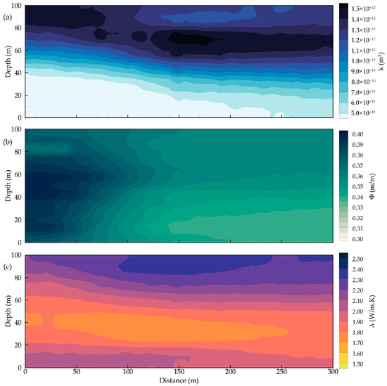
Figure 1.
Schematic representation of the synthetic two-dimensional aquifer for the study (a) permeability, (b) porosity, and (c) thermal conductivity.
Table 2.
Hydrothermal properties in the Simulator for HEat and MAss Transport modeling (SHEMAT).
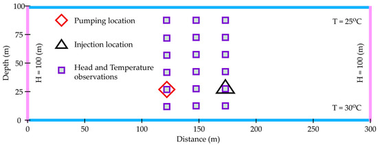
Figure 2.
Schematic representation of the synthetic two-dimensional profile model for the aquifer.
3.2. Generation of Synthetic Observations
The modeling area is discretized into 1200 elements (60 × 20), each with a uniform size of 5 m by 5 m. Figure 2 shows a schematic representation of the synthetic two-dimensional profile aquifer for the locations of injection, pumping, and monitoring wells. Each well is considered fully penetrated, i.e., the well screen is open throughout the entire aquifer. Moreover, the direct measurements of hydrothermal properties along each wellbore are known from the sampled well logs. To make optimal use of information from well hydraulic tests, 5 pneumatic packers are installed in each well to isolate flows from vertical directions. Heat is injected into one of the injection wells at a constant rate of 0.001 m3/s and a temperature of 30 °C for the injected water. There is also a pumping well with a constant pumping rate of 0.001 m3/s. The total simulation time is 1000 days with an interval of 0.1 days. The temperature responses at all 18 observation locations are collected at 0.1, 0.2, 0.3, 0.4, 0.5, 1.0, 1.5, 2.0, 3.0, 5.0, 100, 200, 300, 400, 500, 600, 700, 800, 900, and 1000 days. A total of 18 temperature observation locations were later created for our inverse model to estimate the distributions of permeability, porosity, and thermal conductivity in the modeling area.
4. Results and Discussions
4.1. Parameter Estimation
The hydrothermal parameters shown in Figure 1 are the basis for generating synthetic observation data along the wells. We assume that the synthetic data obtained from the forward model are the observations for the inverse models. Our objective is to assess the accuracy of the inverse models that could reproduce the target hydrothermal parameter fields (or true or reference fields) shown in Figure 1. Figure 3 displays the spatial distributions of permeability, porosity, and thermal conductivity, estimated by using CS (Figure 3a,c,e) and EnKF (Figure 3b,d,e), based on 1000 realizations (MCS) and 1000 ensemble members (EnKF) In this context, the distance between the injection well and the pumping well is 50 m, with the monitoring point located in the middle between the two wells. In general, MCS shows a relatively uniform spatial distribution of hydrothermal properties by comparing the results obtained from EnKF. The high- and low-permeability zones are well reconstructed by MCS and EnKF, particularly the high-permeability zone in Figure 3a and the low-permeability zone in Figure 3b, respectively. Most of the conditioning and measurement points are primarily concentrated in the high-permeability zone. Thus, the spatial distribution of the high-permeability zones is better represented than that of the low-permeability zones. Likewise, the spatial distribution of low porosity zones is concentrated near the measurement points, as shown in Figure 3c,d for MCS and EnKF, respectively. Obviously, the spatial distribution of permeability and porosity zones is controlled by the conditioning points [43,44,45,46]. Meanwhile, the spatial distribution of the thermal conductivity exhibits minimal differences between MCS and EnKF. While MCS shows a smooth thermal conductivity pattern across the domain in Figure 3e, EnKF exhibits slight fluctuations near the injection location in Figure 3f. This can be explained by the fact that temperatures measured at specific points in the EnKF are used to adjust the thermal conductivity during parameter estimation in uncertain, high-stress situations [47,48]. Ultimately, both MCS and EnKF successfully captured the spatial distribution of hydrothermal properties in this scenario, as mentioned above.
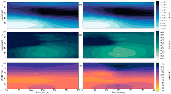
Figure 3.
The distribution of estimated parameters, including (a,b) permeability, (c,d) porosity, and (e,f) thermal conductivity (top, middle, and bottom, respectively) within MCS (left column) and EnKF (right column).
Figure 4 presents a comparative analysis of the estimated versus reference values for three hydrothermal properties, including permeability, porosity, and thermal conductivity in logarithm using stochastic approaches again with MCS (Figure 4a,c,e) and EnKF (Figure 4b,d,f) at 1000 realizations and 1000 ensemble members. In general, all three parameters exhibit a reasonably good agreement between the estimated and reference values. Using Equation (12) to examine the three true and estimated parameters, we obtain the highest correlation coefficient of permeability, 0.95, for both MCS and EnKF. It appears that the simulation performance of MCS and EnKF is equivalent. In addition, MAE and MSE for MCS in Figure 4a are 0.124 and 0.027, while EnKF in Figure 4b is 0.132 and 0.031, respectively. These evaluation metrics further confirm that the MCS and EnKF methods could reconstruct the permeability distribution well when solving the inverse problem [49,50]. With other parameters, the porosity presents an acceptable correlation coefficient of 0.671 for both MCS and EnKF. However, the MAE and MSE for EnKF in Figure 4d are 0.043 and 0.003, respectively. The evaluation metrics for MCS are approximately twice those of EnKF, at 0.076 and 0.007, respectively (Figure 4c). In the models, the measurement dataset (temperature and hydraulic head) should be used to modify the porosity distribution, along with the conditioning points, to improve prediction results. This information reinforces the statement about the accuracy of EnKF in parameter estimation compared to MCS, as previously discussed for Figure 3d. The two stochastic inverse models are effective at representing the patterns of these parameters, with high correlation coefficients of 0.913 and 0.926 (see Figure 4e,f). Moreover, the calculated MAE and MSE values are low for the three predicted hydrothermal parameters. These values are 0.030 and 0.002 for MCS (see Figure 4e) and 0.045 and 0.003 for EnKF (Figure 4f). Although the correlation coefficient is better for EnKF than that for MCS. However, the MCS yields lower MAE and MSE than the EnKF. Based on the general concepts of the two models, the observed data are used to update parameter estimates during the updating process. In Figure 4e,f, the overall performance of MCS and EnKF shows that the distribution of low thermal conductivity values is generally underestimated, while the distribution of high thermal conductivity values is overestimated, as indicated by comparisons between estimated and reference thermal conductivities across different elements.
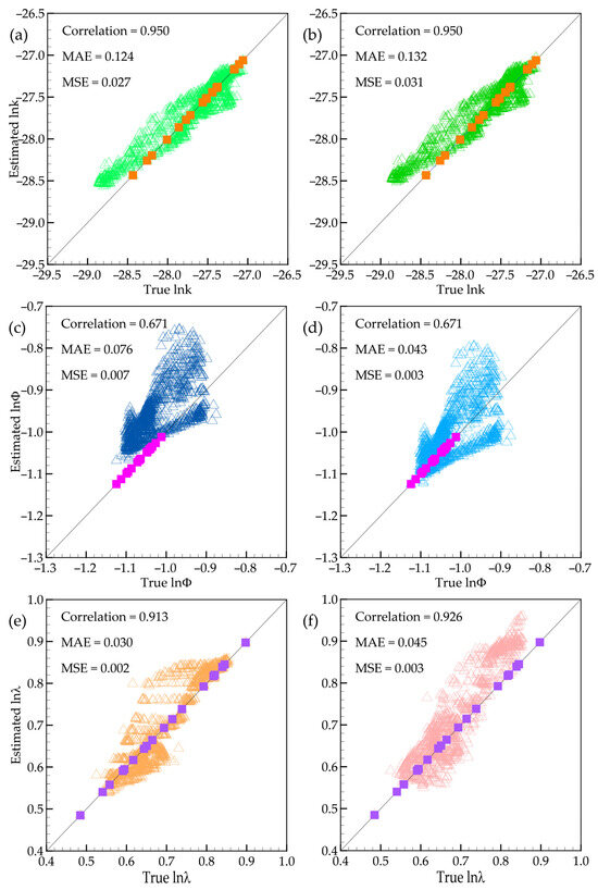
Figure 4.
The scatter plot of parameters estimation, including (a,b) permeability, (c,d) porosity, and (e,f) thermal conductivity in natural logarithm scale (top, middle, and bottom, respectively) within MCS (left column) and EnKF (right column).
Two significant indicators for MCS and EnKF are the number of realizations and the ensemble size, referred to as the number of samples in this study. Under this scenario, we run several simulations with sample sizes ranging from 100 to 2000. Then, we use the criteria to evaluate the simulation performance of MCS and EnKF for hydrothermal properties, as shown in Figure 5. The correlation coefficients decrease for permeability, porosity, and thermal conductivity when 1000 samples are used, as shown in Figure 5a,d,g, respectively. Further evaluation metrics, such as MAE and MSE, are also maintained at 1000 samples in the other sub-graphs in Figure 5, except for the list of figures mentioned above. This figure reinforces the statement that the stochastic inversion model successfully balances the prediction results at 1000 samples, supporting the discussion in Figure 4 above.
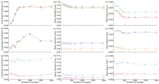
Figure 5.
The simulation performance evaluation indicators of parameter estimation including (a–c) permeability, (d–f) porosity, and (g–i) thermal conductivity in natural logarithm scale (top, middle, and bottom, respectively) with correlation coefficient (left), MAE (center), and MSE (right) using MCS (dash line) and EnKF (solid line).
The current literature indicates a limited number of studies highlighting the effectiveness of the EnKF compared to MCS for parameter estimation, particularly in terms of computational time. Thus, a comparative analysis of the computational efficiency and time requirements of the MCS and EnKF with varying sample sizes (100–2000 realizations for MCS and EnKF, respectively) is presented in Figure 6. Note that the comparison was based on the models executed with the same computer system and hardware. The computational time requirements reveal that MCS exhibits exponential growth, with execution time increasing substantially beyond 500 realizations. In contrast, EnKF demonstrates linear scaling, with relatively small increases in computational time over the entire tested range. The results indicate that EnKF maintains a computational advantage of more than six times at smaller ensemble sizes (at 100 realizations for MCS), with consistent superiority throughout the parameter space, despite decreasing efficiency ratios up to 2000 ensemble sizes. Although the relative advantage of EnKF decreases slightly as ensemble size increases, it consistently outperforms MCS across all tested scenarios. These results demonstrate that EnKF is a relatively cost-effective approach for handling large-scale uncertainty and data integration, particularly when simulations are computationally expensive.
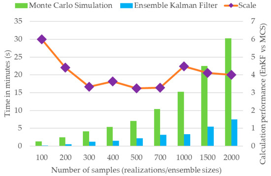
Figure 6.
Comparison of simulation performance with variations in different numbers of samples between the MCS and EnKF. The variations in scale values indicate the ratios of computational times required for MCS and EnKF to complete specific numbers of realizations or ensemble sizes.
4.2. Model Uncertainties
To quantify the performance of the MCS and EnKF in parameter estimation, five scenarios are created. Herein, we have already defined a monitoring well at 150 m as the center section of the aquifer profile. Next, we gradually increase the distance between the injection well and the pumping well with intervals of 50 m (scenario A), 100 m (scenario B), 150 m (scenario C), 200 m (scenario D), and 250 m (scenario E). The conceptual model for scenario A serves as the base case for our previous discussion (see Figure 2). Similar to scenario A, the injection well and pumping are shifted to the left and right sides of the aquifer profile, respectively, as shown in Figure 7. Other model settings are fixed based on scenario A, including boundary and initial conditions, hydrothermal properties, injection and pumping rates, and numerical considerations.
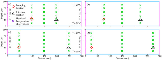
Figure 7.
Schematic representation of the synthetic two-dimensional profile aquifer for evaluating the influence of well distances on the estimation results: (a) scenario B, (b) scenario C, (c) scenario D, and (d) scenario E.
4.2.1. Optimal Network of Monitoring Wells
To quantify the performance of the MCS and EnKF in parameter estimation, five scenarios are created. Herein, we have already defined a monitoring well at 150 m as the center section of the aquifer profile. Next, we gradually increase the distance between the injection well and the pumping well with intervals of 50 m (scenario A), 100 m (scenario B), 150 m (scenario C), 200 m (scenario D), and 250 m (scenario E).
Using stochastic methods, we have extended benchmarking across multiple scenarios to quantify the uncertainties associated with MCS and EnKF in parameter estimation. In this situation, we also examine the impact of the number of samples (i.e., the number of realizations and ensemble size for MCS and EnKF, respectively). This will re-examine the effect of sample size and determine the optimal sample sizes.
A key hydrothermal property is permeability [42,49,50,51], which yields excellent estimates, as shown in Figure 8. In this figure, the color-coded bars illustrate the increasing number of samples, ranging from 100 to 2000, with MCS and EnKF shown in the left- and right-hand columns of each subplot, respectively. The correlation coefficient tends to stabilize at 1000 samples, indicated by the red color for all scenarios with MCS and EnKF. This point is supported by the earlier discussion, which suggests 1000 samples is a suitable number for both MCS and EnKF, while the well spacing between scenarios A and E gradually increases from 50 m to 250 m. Similar to this trend, the MAE and MSE have acceptable values at 1000 samples. Along with this trend, MAE and MSE have acceptable values for 1000 samples. Upon examining all measured values, it is evident that the scenarios in C yield favorable outcomes for parameter estimation and demonstrate a robust correlation of 0.98 across all stochastic approaches. With a gradual extension of well spacing beyond 150 m, the simulated results showed minimal deviations. Therefore, we can conclude that the optimal distance between injection and pumping wells should be about 150 m, with a monitoring well positioned between them. This arrangement optimizes the monitoring of hydraulic responses and increases the accuracy of the estimated parameters. Additionally, maintaining this distance can help mitigate potential interference effects between the injection and pumping wells and ensure more reliable data collection.
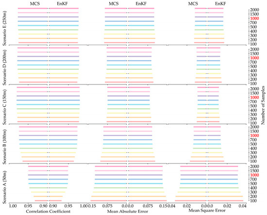
Figure 8.
The comparison of estimation performance for permeability in natural logarithm scale using MCS (left side of subplot) and EnKF (right side of subplot) with correlation coefficient (left column), MAE (center column), and MSE (right column) for the five scenarios (from bottom to top).
Porosity plays an essential role in the storage and release of heat in soil, a frequently observed parameter in heat transport processes in heterogeneous porous media and confined aquifer systems. Scenario C represents the best scenario for porosity prediction in Figure 9. Conversely, scenario A is the worst-case scenario, characterized by the lowest correlation coefficient and the highest MAE and MSE. The simulation results improve as the distance between wells is gradually increased in 50 m intervals. From this perspective, scenario C is once again considered satisfactory for parameter estimation of the predicted porosity. The correlation coefficient, MAE, and MSE stabilize at 1000 samples in this scenario, with 0.8974, 0.0763, and 0.0071 for MCS, and 0.8974, 0.0325, and 0.0022 for EnKF, respectively. In this situation, EnKF estimates the porosity field with higher accuracy than MCS, while the correlation coefficient remains unchanged. Such results might be due to the updating process introduced in the EnKF for parameter estimation [11,52]. This iterative refinement allows the EnKF to better align model estimates with observed data, resulting in improved reliability of the porosity estimates. Consequently, the results suggest that incorporating observational data through methods such as EnKF could significantly improve predictive performance in geostatistical modeling [53,54].
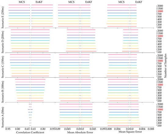
Figure 9.
The summary of estimation performance for porosity in natural logarithm scale using MCS (left side of subplot) and EnKF (right side of subplot) with correlation coefficient (left), MAE (center), and MSE (right) for five scenarios with increasing well spacing (from bottom to top).
When applying the stochastic inversion procedure for parameter estimation, we found several interesting points. Figure 10 shows how the stochastic inversion of thermal conductivity with MCS and EnKF works as the distance between wells increases from 50 m (scenario A, a typical case) to 250 m (scenario E). The correlation coefficient stabilizes in scenario D for MCS, whereas it gradually decreases for EnKF as the well spacing increases from 50 m to 250 m, using 1000 samples. Similarly, MAE and MSE begin to show signs of imbalance at a well spacing of 150 m, as observed in scenario C for MCS. Meanwhile, MAE and MSE for EnKF fluctuate within the ranges of 0.04 to 0.06 and 0.003 to 0.005, respectively. The difference between MCS and EnKF is minimal, with a difference of 0.01 for MAE and 0.001 for MSE. Therefore, the accuracy of thermal conductivity prediction should primarily focus on the correlation coefficient. In this context, we illustrate the differences between the two stochastic approaches with respect to the impact of well spacing. Increasing well spacing has made it more challenging to transfer the temperature from the injection well to the pumping well. MCS uses geological structures to estimate thermal conductivity, whereas EnKF relies on observations to refine its parameter estimates. This EnKF update, influenced by the significant temperature difference, leads to discrepancies due to the considerable distance between the injection and pumping wells. Consequently, it may be necessary to adjust the well spacing or use additional monitoring techniques to improve the accuracy of thermal conductivity estimation. Based on observations from the numerical experiments, we conclude that injection, pumping, and monitoring wells should be evenly distributed throughout the domain. However, the condition would vary depending on the stress induced by the injection and pumping wells and the location of the monitoring well.
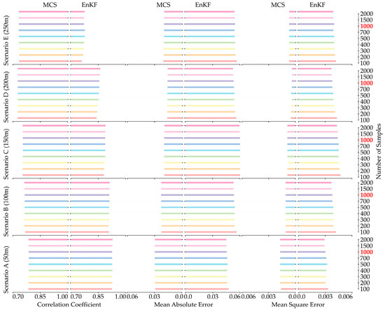
Figure 10.
The summary of estimation performance for thermal conductivity in natural logarithm scale using MCS (left side of each column) and EnKF (right side of each column) with correlation coefficient (left column), MAE (center column), and MSE (right column) during the five scenarios with increasing well spacing (from bottom to top).
4.2.2. Optimal Correlation Length of Stochastic Inversion Model
In the previous discussion, we emphasized the important role of the distribution of monitoring well networks, including injection wells, pumping wells, and monitoring wells. Here, we continue to explore the impact of the correlation length in stochastic inversion modeling, which is crucial for accurately representing the geostatistical structure in parameter estimation. In this section, we modify the correlation length range from 60 m to 240 m using a 60 m interval for the horizontal correlation length (X), and include a list of lengths at 10 m, 20 m, 30 m, and 50 m for the depth correlation length (Z) in the synthetic aquifer profile. Additionally, we predict the hydrothermal properties based on all scenarios described in the previous section.
Following the previous section, we start with estimating permeability, a key factor influencing the hydrothermal properties of the aquifer system. The sequential color bars in Figure 11 indicate high and low correlation of coefficients, represented by yellow and red colors, respectively. Notably, high correlation coefficients are observed at horizontal correlation lengths of x = 120 m and 240 m, as well as at depth correlation lengths of z = 30 m and 50 m. The results suggest that the horizontal correlation length should range from 0.4 to 0.8 times the total length of the horizontal aquifer profile, while the depth correlation length should range from 0.3 to 0.5 times the total length of the depth aquifer profile. In line with the distribution of the correlation coefficient for permeability, both MAE and MSE exhibit low values at horizontal correlation lengths of x = 120 m and 240 m, as well as at depth correlation lengths of z = 30 m and 50 m, as depicted in Figure 11. The low and high values are indicated by sequential colors: blue and spring green for MAE and cyan and pink for MSE. Additionally, scenario C demonstrates stable parameter estimation across all evaluation metrics, with no changes observed as the well spacing increased. We reiterate that the optimal distance between the injection well and the pumping well is 150 m, as shown in scenario C, with correlation lengths ranging from 120 m to 240 m for x and from 30 m to 50 m for z, reflecting reasonable distributions of parameter estimates. Clearly, the two stochastic approaches yielded similar simulation results based on the evaluation metrics discussed in the previous section (e.g., Figure 8).
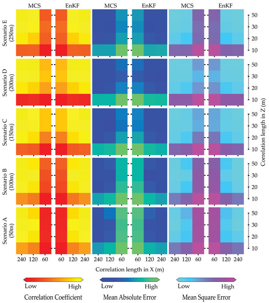
Figure 11.
Summary of performance evaluation for permeability in natural logarithm scales using MCS and EnKF with correlation coefficient (left), MAE (center), and MSE (right) for five scenarios with increasing well spacing (from bottom to top) under the variation in the correlation lengths in X- and Y-directions based on 1000 samples.
Figure 12 illustrates the evaluation metrics for porosity estimation. The color bar display is consistent with Figure 11 for the evaluation metric of permeability prediction. Repeatedly, the EnKF shows better porosity estimation than the MCS on the evaluation criteria. For scenario C, the correlation coefficient is predominantly yellow, indicating a high EnKF value at a horizontal correlation length of x = 240 m, whereas MCS shows the opposite. The MAE and MSE are displayed in blue and cyan colors, respectively, for low values. Furthermore, EnKF used observed data to calibrate porosity and improve parameter estimation accuracy. When we increase the distance, as in scenarios D and E, the evaluation metrics do not change significantly. Hence, we again demonstrate that the reasonable distance between the injection well and the pumping well is 150 m, with a monitoring well located at the center of the two wells. In scenarios A and B, where the well spacing is smaller, the porosity prediction shows low accuracy, as indicated by the high MAE and MSE values in spring green and pink, particularly for MCS.
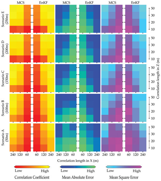
Figure 12.
Summary of performance evaluation for porosity in natural logarithm scales using MCS and EnKF with correlation coefficient (left), MAE (center), and MSE (right) for five scenarios with increasing well spacing (from bottom to top) under the variation in the correlation lengths in X- and Y-directions based on 1000 samples.
Figure 13 displays the evaluation criteria for thermal conductivity prediction using MCS and EnKF. Note that the color bar display is compatible with Figure 11 and Figure 12. In general, MCS shows the brightest yellow color, indicating a strong correlation, suggesting that it can estimate thermal conductivity accurately at x = 120 m and 240 m for horizontal distance, and at z = 20 m, 30 m, and 50 m for depth. The situation is similar to the MAE and MSE; the bluest and cyan colors indicate the low value, accordingly. Based on the previous discussion, the MCS did not utilize the observation dataset and instead focused solely on the geostatistical structure. Hence, the MCS is superior to the EnKF in this situation. Additionally, the good simulation for thermal conductivity occurs at x = 60 m and z = 10, corresponding to the horizontal and depth correlation lengths in scenarios C, D, and E. This can be explained by the fact that EnKF utilizes observational data, such as temperature measurements and conditioning points (e.g., thermal conductivity, which is considered reliable data during updates), at a small correlation length. The influence of the water temperature from the injection well to the pumping well is insufficient due to the increasing well spacing. This limited influence highlights the challenges of accurately modeling thermal dynamics in scenarios C, D, and E, where the distance between wells strongly influences the spatial distribution of temperature. As a result, the effectiveness of the EnKF in integrating observational data decreases, so a more refined approach is required to account for the complex interactions at greater distances. The analysis also indicates that selecting appropriate well distances (or monitoring locations) is crucial for obtaining accurate estimates of target hydrothermal properties. For most practical problems, the resources are often limited. The determination of monitoring wells for parameter estimations might require other techniques such as geophysical surveys to map the possible structure of the underground material. The images from the geophysical surveys could be the important reference to determine the installation of the monitoring network [16,55].
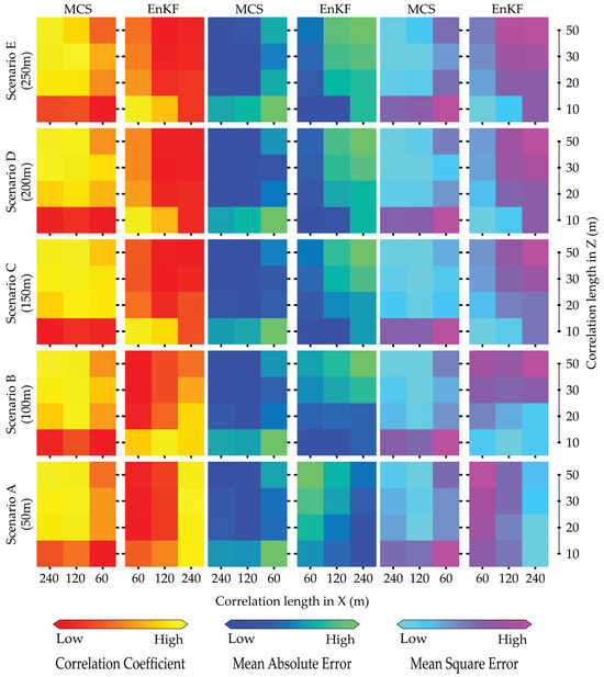
Figure 13.
Summary of performance evaluation for thermal conductivity in natural logarithm scales using MCS and EnKF with correlation coefficient (left), MAE (center), and MSE (right) for five scenarios with in-creasing well spacing (from bottom to top) under the variation in the correlation lengths in X- and Y-directions based on 1000 samples (For interpretation of the colors in the figure(s), the reader is referred to the web version of this article).
5. Practical Applications and Future Research Perspectives
Stochastic inversion of heat transport in heterogeneous porous media serves several important scientific and engineering purposes, particularly in subsurface applications such as geothermal energy, radioactive waste disposal, hydrogeology, and environmental remediation. Environmental remediation efforts often rely on accurate modeling of heat transport to evaluate the effectiveness of various treatment strategies [56,57]. By employing stochastic inversion techniques, researchers can gain a better understanding of the complex interactions within porous media, leading to more effective solutions for mitigating contamination and restoring affected environments.
To date, various methods have been developed to solve the stochastic inversion of heat transport problems in heterogeneous porous media, particularly data assimilation. Many studies have demonstrated that EnKF is a powerful tool for parameter estimation, both for synthetic cases [53] and for specific sites. For instance, EnKF has been successfully implemented for permeability prediction and uncertainty quantification at Altona Flat Rocks region in the USA [58] or Soultz-sous-Forêts in France [11,17]. All studies show that EnKF performed precisely as predicted, and the associated uncertainty was evaluated using the ensembles of posterior models obtained. It can be seen that the potential of data assimilation is immense for solving stochastic inversions in heat transport. Hence, this study suggests that further data assimilation methods should be explored to investigate the geothermal system, such as ensemble smoothing and ensemble learning. Additionally, in situ observations are required and play an essential role in conditioning the state variables in data assimilation. High spatial- and temporal-resolution monitoring systems at sites could also support site characterization of a geothermal system.
In general, the primary drawback of data assimilation methods is the large number of observations required for the updating processes. To overcome this barrier, with the rapid advances in the era of artificial intelligence, surrogate modeling is emerging as an alternative solution for studying subsurface thermal systems, particularly geothermal systems. Several studies use Convolutional Variational Auto-Encoders to predict thermal performance [59] or Physics-Informed Machine Learning to manage enhanced geothermal systems [57]. Dashtgoli et al. [60] implemented XGBoost to evaluate the accuracy of geothermal temperature estimation in the Lower Friulian Plain in Northeastern Italy and compared it with MCS. Very little research has been conducted to explore the potential of surrogate modeling for solving both forward and inverse heat transport in heterogeneous porous media. Therefore, it is necessary to conduct more in-depth studies using Offline Reinforcement Learning, Bayesian deep learning, and Generative Adversarial Networks to fully exploit their potential in this field.
In addition to the accuracy of the methods mentioned above, the consideration of computation time is very important. As computational demands increase, conventional computational approaches become increasingly inadequate due to the growing model sizes and the need for high detail density and substantial amounts of input data. This requirement has prompted the further development of quantum computing to address these issues. Currently, there is a lack of research that successfully applies quantum computing to real-world issues. Consequently, additional research is necessary to explore the integration of machine learning and data assimilation with quantum computing as a viable option for the future.
6. Conclusions
In this study, the stochastic inversion techniques are used to conduct hydrothermal parameter estimations in heterogeneous porous media. Furthermore, we analyze in depth various factors influencing the prediction of the parameters based on real application knowledge and specific algorithms for capturing subsurface heterogeneities and estimating model uncertainty. The following are the conclusions based on the study:
- (a)
- Hydro-thermal properties are fully captured by implementing both MCS and EnKF, including permeability, porosity, and thermal conductivity. EnKF generally performs better than MCS because it uses simultaneous observational data to update parameter estimates and can perform calculations up to six times faster than MCS.
- (b)
- An optimal network of monitoring wells is proposed, with an appropriate distance between the injection and the pumping wells of at least half the length of the area. Additionally, an observation well is located between these two wells to ensure the observations are evenly distributed across the domain.
- (c)
- The monitoring network to capture hydrothermal properties in a heterogeneous aquifer relies on information about the geostatistical structure for the target hydrothermal properties. The monitoring distance needs to be smaller than the correlation lengths of the hydrothermal properties. However, due to limited resources for developing a monitoring network, geophysical surveys might be helpful in supporting its design.
- (d)
- Further approaches, such as data assimilation and machine learning techniques, should be considered for solving forward and inverse problems in geothermal systems in heterogeneous porous media. Quantum computing has the potential to address the challenges posed by high computational demands.
Overall, parameter estimation and uncertainty quantification using stochastic approaches enhance the robustness of model predictions and enable better decision-making in reservoir management. Future work should focus on improving the computational efficiency of these methods and refining the integration of observational data to further reduce uncertainty in complex geothermal systems.
Author Contributions
D.T.T.T.: Writing—original draft, Conceptualization, Modeling, Validation. C.-F.N.: Conceptualization, Writing—review and editing, Funding acquisition. N.H.H.: Conceptualization, Writing—review and editing. H.-S.V.: Writing—review and editing. T.-V.-T.N.: Writing—review and editing. L.N.Y.: Writing—review and editing. M.-Q.D.: Writing—review and editing. All authors have read and agreed to the published version of the manuscript.
Funding
This research was partially supported by the National Science and Technology Council, Taiwan, under grants NSTC 111-2621-M-008-003, NSTC 112-MOEA-M-008-001, NSTC 112-2123-M-008-001, NSTC 112-2122-M-007-002, and NSTC 113-MOEA-M-008-001.
Data Availability Statement
The original contributions presented in the study are included in the article; further inquiries can be directed to the corresponding author.
Acknowledgments
During the preparation of this manuscript/study, the authors used SHEMAT-suite version 9 (accessed on 25 October 2025) for the purposes of simulations. The authors have reviewed and edited the output and take full responsibility for the content of this publication.
Conflicts of Interest
The authors declare no conflicts of interest.
References
- Shortall, R.; Davidsdottir, B.; Axelsson, G. Geothermal energy for sustainable development: A review of sustainability impacts and assessment frameworks. Renew. Sustain. Energy Rev. 2015, 44, 391–406. [Google Scholar] [CrossRef]
- Idroes, G.M.; Hardi, I.; Hilal, I.S.; Utami, R.T.; Noviandy, T.R.; Idroes, R. Economic growth and environmental impact: Assessing the role of geothermal energy in developing and developed countries. Innov. Green Dev. 2014, 3, 100144. [Google Scholar] [CrossRef]
- Liu, G.; Zhou, B.; Liao, S. Inverting methods for thermal reservoir evaluation of enhanced geothermal system. Renew. Sustain. Energy Rev. 2018, 82, 471–476. [Google Scholar] [CrossRef]
- Piechowski, M. Heat and mass transfer model of a ground heat exchanger: Validation and sensitivity analysis. Int. J. Energy Res. 1998, 22, 965–979. [Google Scholar] [CrossRef]
- Jia, G.S.; Ma, Z.D.; Xia, Z.H.; Wang, J.W.; Zhang, Y.P.; Jin, L.W. Influence of groundwater flow on the ground heat exchanger performance and ground temperature distributions: A comprehensive review of analytical, numerical and experimental studies. Geothermics 2022, 100, 102342. [Google Scholar] [CrossRef]
- Kim, D.; Kim, G.; Kim, D.; Baek, H. Experimental and numerical investigation of thermal properties of cement-based grouts used for vertical ground heat exchanger. Renew. Energy 2017, 112, 260–267. [Google Scholar] [CrossRef]
- Zhang, Z.; Jafarpour, B.; Li, L. Inference of permeability heterogeneity from joint inversion of transient flow and temperature data. Water Resour. Res. 2014, 50, 4710–4725. [Google Scholar] [CrossRef]
- Suzuki, A.; Fukui, K.I.; Onodera, S.; Ishizaki, J.; Hashida, T. Data-driven geothermal reservoir modeling: Estimating permeability distributions by machine learning. Geosciences 2022, 12, 130. [Google Scholar] [CrossRef]
- Liu, Q.; Wang, M. Numerical investigation of water migration in a closed unsaturated expansive clay system. Bull. Eng. Geol. Environ. 2023, 82, 202. [Google Scholar] [CrossRef]
- Manzella, A. Technological challenges in exploration and investigation of EGS and UGR. In Proceedings of the 2010 World Geothermal Congress, Bali, Indonesia, 25–30 April 2010; Horne, R., Ed.; International Geothermal Association: Bochum, Germany, 2010. [Google Scholar]
- Vogt, C.; Marquart, G.; Kosack, C.; Wolf, A.; Clauser, C. Estimating the permeability distribution and its uncertainty at the EGS demonstration reservoir Soultz-sous-Forêts using the ensemble Kalman filter. Water Resour. Res. 2012, 48, W08517. [Google Scholar] [CrossRef]
- Shi, C.; Wang, Y. Data-driven construction of Three-dimensional subsurface geological models from limited Site-specific boreholes and prior geological knowledge for underground digital twin. Tunn. Undergr. Space Technol. 2022, 126, 104493. [Google Scholar] [CrossRef]
- Franssen, H.H.; Alcolea, A.; Riva, M.; Bakr, M.; Van der Wiel, N.; Stauffer, F.; Guadagnini, A. A comparison of seven methods for the inverse modelling of groundwater flow. Application to the characterisation of well catchments. Adv. Water Resour. 2009, 32, 851–872. [Google Scholar] [CrossRef]
- Shcherbakov, R. A stochastic model for induced seismicity at the geothermal systems: A case of the Geysers. Seismol. Res. Lett. 2024, 95, 3545–3556. [Google Scholar] [CrossRef]
- de Beer, A.; Bjarkason, E.K.; Gravatt, M.; Nicholson, R.; O’Sullivan, J.P.; O’Sullivan, M.J.; Maclaren, O.J. Ensemble Kalman inversion for geothermal reservoir modelling. Geophys. J. Int. 2025, 241, 580–605. [Google Scholar] [CrossRef]
- Vogt, C.; Mottaghy, D.; Wolf, A.; Rath, V.; Pechnig, R.; Clauser, C. Reducing temperature uncertainties by stochastic geothermal reservoir modelling. Geophys. J. Int. 2010, 181, 321–333. [Google Scholar] [CrossRef][Green Version]
- Vogt, C.; Kosack, C.; Marquart, G. Stochastic inversion of the tracer experiment of the enhanced geothermal system demonstration reservoir in Soultz-sous-Forêts—Revealing pathways and estimating permeability distribution. Geothermics 2012, 42, 1–12. [Google Scholar] [CrossRef]
- Kaplan, D. On the quantification of model uncertainty: A Bayesian perspective. Psychometrika 2021, 86, 215–238. [Google Scholar] [CrossRef]
- Acar, E.; Bayrak, G.; Jung, Y.; Lee, I.; Ramu, P.; Ravichandran, S.S. Modeling, analysis, and optimization under uncertainties: A review. Struct. Multidiscip. Optim. 2021, 64, 2909–2945. [Google Scholar] [CrossRef]
- Berardi, M.; Andrisani, A.; Lopez, L.; Vurro, M. A new data assimilation technique based on ensemble Kalman filter and Brownian bridges: An application to Richards’ equation. Comput. Phys. Commun. 2016, 208, 43–53. [Google Scholar] [CrossRef]
- Jamal, A.; Linker, R. Inflation method based on confidence intervals for data assimilation in soil hydrology using the ensemble Kalman filter. Vadose Zone J. 2020, 19, e20000. [Google Scholar] [CrossRef]
- Zhou, D.; Tatomir, A.; Sauter, M. Thermo-hydro-mechanical modelling study of heat extraction and flow processes in enhanced geothermal systems. Adv. Geosci. 2021, 54, 229–240. [Google Scholar] [CrossRef]
- Crestani, E.; Camporese, M.; Baú, D.; Salandin, P. Ensemble Kalman filter versus ensemble smoother for assessing hydraulic conductivity via tracer test data assimilation. Hydrol. Earth Syst. Sci. 2013, 17, 1517–1531. [Google Scholar] [CrossRef]
- Keller, J.; Rath, V.; Bruckmann, J.; Mottaghy, D.; Clauser, C.; Wolf, A.; Seidler, R.; Bücker, H.M.; Klitzsch, N. SHEMAT-Suite: An open-source code for simulating flow, heat and species transport in porous media. SoftwareX 2020, 12, 100533. [Google Scholar] [CrossRef]
- Clauser, C. (Ed.) Numerical Simulation of Reactive Flow in Hot Aquifers—SHEMAT and Processing SHEMAT; Springer: New York, NY, USA, 2003. [Google Scholar] [CrossRef]
- Beardsmore, G.R.; Cull, J.P. Crustal Heat Flow; Cambridge University Press: Cambridge, UK, 2001. [Google Scholar] [CrossRef]
- Clauser, C. Thermal storage and transport properties of rocks, II: Thermal conductivity and diffusivity. In Encyclopedia of Solid Earth Geophysics; Gupta, H.K., Ed.; Springer: Berlin/Heidelberg, Germany, 2011; Volume 2, pp. 1431–1448. [Google Scholar]
- Phillips, S.L.; Igbene, A.; Fair, J.A.; Ozbek, H.; Tavana, M. A Technical Data Book for Geothermal Energy Utilization; Technical Report 12810 UC-66a; Lawrence Berkeley Laboratory, University of California: Berkeley, CA, USA, 1981. [Google Scholar] [CrossRef]
- Zyvoloski, G.A.; Robinson, B.A.; Dash, Z.V.; Trease, L.L. Models and Methods Summary for the FEHMN Application; No. LA-UR-94-3787-Rev. 1; Los Alamos National Lab (LANL): Los Alamos, NM, USA, 1996. [Google Scholar] [CrossRef][Green Version]
- Lynch, D.R. Numerical Partial Differential Equations for Environmental Scientists and Engineers: A First Practical Course; Springer: New York, NY, USA, 2005. [Google Scholar] [CrossRef]
- Huyakorn, P.S.; Pinder, G.F. Computational Methods in Subsurface Flow; Academic Press: Cambridge, MA, USA, 2012. [Google Scholar] [CrossRef]
- Deutsch, C.V.; Journel, A.G. GSLIB: Geostatistical Software Library And User’s Guide, 2nd ed.; Oxford University Press: New York, NY, USA, 1998; p. 369. [Google Scholar] [CrossRef]
- Rath, V.; Wolf, A.; Bücker, H.M. Joint three-dimensional inversion of coupled groundwater flow and heat transfer based on automatic differentiation: Sensitivity calculation, verification, and synthetic examples. Geophys. J. Int. 2006, 167, 453–466. [Google Scholar] [CrossRef]
- Chen, Y.; Zhang, D. Data assimilation for transient flow in geologic formations via ensemble Kalman filter. Adv. Water Resour. 2006, 29, 1107–1122. [Google Scholar] [CrossRef]
- Kalman, R.E. A new approach to linear filtering and prediction problems. J. Basic Eng. 1960, 82, 35–45. [Google Scholar] [CrossRef]
- Aanonsen, S.I.; Nævdal, G.; Oliver, D.S.; Reynolds, A.C.; Vallès, B. The Ensemble Kalman filter in reservoir engineering—A review. SPE J. 2009, 14, 393–412. [Google Scholar] [CrossRef]
- Oliver, D.S.; Chen, Y. Recent progress on reservoir history matching: A review. Comput. Geosci. 2011, 15, 185–221. [Google Scholar] [CrossRef]
- Burgers, G.; Jan van Leeuwen, P.; Evensen, G. Analysis scheme in the ensemble Kalman filter. Mon. Weather Rev. 1998, 126, 1719–1724. [Google Scholar] [CrossRef]
- Evensen, G. The Ensemble Kalman Filter: Theoretical formulation and practical implementation. Ocean Dyn. 2003, 53, 343–367. [Google Scholar] [CrossRef]
- Franssen, H.H.; Kinzelbach, W. Ensemble Kalman filtering versus sequential self-calibration for inverse modelling of dynamic groundwater flow systems. J. Hydrol. 2008, 365, 261–274. [Google Scholar] [CrossRef]
- Krymskaya, M.V.; Hanea, R.G.; Verlaan, M. An iterative ensemble Kalman filter for reservoir engineering applications. Comput. Geosci. 2008, 13, 235–244. [Google Scholar] [CrossRef]
- Bauer, J.F.; Krumbholz, M.; Luijendijk, E.; Tanner, D.C. A numerical sensitivity study of how permeability, porosity, geological structure, and hydraulic gradient control the lifetime of a geothermal reservoir. Solid Earth 2019, 10, 2115–2135. [Google Scholar] [CrossRef]
- Ni, C.F.; Yeh, T.C.J. Stochastic inversion of pneumatic cross-hole tests and barometric pressure fluctuations in heterogeneous unsaturated formations. Adv. Water Resour. 2008, 31, 1708–1718. [Google Scholar] [CrossRef]
- Ni, C.F.; Yeh, T.C.J.; Chen, J.S. Cost-effective hydraulic tomography surveys for predicting flow and transport in heterogeneous aquifers. Environ. Sci. Technol. 2009, 43, 3720–3727. [Google Scholar] [CrossRef] [PubMed]
- Yeh, T.C.J.; Gutjahr, A.L.; Jin, M. An iterative cokriging-like technique for groundwater flow modeling. Groundwater 1995, 33, 33–41. [Google Scholar] [CrossRef]
- Yeh, T.C.J.; Liu, S. Hydraulic tomography: Development of a new aquifer test method. Water Resour. Res. 2000, 36, 2095–2105. [Google Scholar] [CrossRef]
- Li, L.; Zhou, H.; Gómez-Hernández, J.J.; Franssen, H.H. Jointly mapping hydraulic conductivity and porosity by assimilating concentration data via ensemble Kalman filter. J. Hydrol. 2012, 428–429, 152–169. [Google Scholar] [CrossRef]
- Xu, T.; Gómez-Hernández, J.J. Joint identification of contaminant source location, initial release time, and initial solute concentration in an aquifer via ensemble Kalman filtering. Water Resour. Res. 2016, 52, 6587–6595. [Google Scholar] [CrossRef]
- Wang, Z.; Liu, S.; Li, H.; Liu, J.; Sun, W.; Xu, J.; Wang, X. CO2 storage in saline aquifers: A simulation on quantifying the impact of permeability heterogeneity. J. Clean. Prod. 2024, 471, 143415. [Google Scholar] [CrossRef]
- Catinat, M.; Fleury, M.; Brigaud, B.; Antics, M.; Ungemach, P. Estimating permeability in a limestone geothermal reservoir from NMR laboratory experiments. Geothermics 2023, 111, 102707. [Google Scholar] [CrossRef]
- Kristensen, L.; Hjuler, M.L.; Frykman, P.; Olivarius, M.; Weibel, R.; Nielsen, L.H.; Mathiesen, A. Pre-drilling assessments of average porosity and permeability in the geothermal reservoirs of the Danish area. Geotherm. Energy 2016, 4, 6. [Google Scholar] [CrossRef]
- Rajabi, M.M.; Chen, M. Dynamical modeling of a geothermal system to predict hot spring behavior. Model. Earth Syst. Environ. 2023, 9, 3085–3093. [Google Scholar] [CrossRef]
- Marquart, G.; Vogt, C.; Klein, C.; Widera, A. Estimation of geothermal reservoir properties using the Ensemble Kalman Filter. Energy Procedia 2013, 40, 117–126. [Google Scholar] [CrossRef][Green Version]
- Godoy, V.A.; Napa-García, G.F.; Gómez-Hernández, J.J. Ensemble smoother with multiple data assimilation as a tool for curve fitting and parameter uncertainty characterization: Example applications to fit nonlinear sorption isotherms. Math. Geosci. 2022, 54, 807–825. [Google Scholar] [CrossRef]
- Ye, Z.; Wang, J.G. Uncertainty analysis for heat extraction performance from a stimulated geothermal reservoir with the diminishing feature of permeability enhancement. Geothermics 2022, 100, 102339. [Google Scholar] [CrossRef]
- Abrasaldo, P.M.B. Machine Learning and Time-Series Analytics Applied to Geothermal Energy Operations. Doctoral Dissertation, The University of Auckland, Auckland, New Zealand, 2024. [Google Scholar]
- Yan, B.; Xu, Z.; Gudala, M.; Tariq, Z.; Sun, S.; Finkbeiner, T. Physics-informed machine learning for reservoir management of enhanced geothermal systems. Geoenergy Sci. Eng. 2024, 234, 212663. [Google Scholar] [CrossRef]
- Wu, H.; Fu, P.; Hawkins, A.J.; Tang, H.; Morris, J.P. Predicting thermal performance of an enhanced geothermal system from tracer tests in a data assimilation framework. Water Resour. Res. 2021, 57, e2021WR030987. [Google Scholar] [CrossRef]
- Chen, C.; Deng, Y.; Ma, H.; Kang, X.; Ma, L.; Qian, J. Deep learning-based inversion framework by assimilating hydrogeological and geophysical data for an enhanced geothermal system characterization and thermal performance prediction. Energy 2024, 302, 131713. [Google Scholar] [CrossRef]
- Dashtgoli, D.S.; Giustiniani, M.; Busetti, M.; Cherubini, C. Artificial intelligence applications for accurate geothermal temperature prediction in the lower Friulian Plain (North-Eastern Italy). J. Clean. Prod. 2024, 460, 142452. [Google Scholar] [CrossRef]


Disclaimer/Publisher’s Note: The statements, opinions and data contained in all publications are solely those of the individual author(s) and contributor(s) and not of MDPI and/or the editor(s). MDPI and/or the editor(s) disclaim responsibility for any injury to people or property resulting from any ideas, methods, instructions or products referred to in the content. |
© 2025 by the authors. Licensee MDPI, Basel, Switzerland. This article is an open access article distributed under the terms and conditions of the Creative Commons Attribution (CC BY) license (https://creativecommons.org/licenses/by/4.0/).