Abstract
Climate change and water scarcity are major threats to the sustainability of wheat production in Mediterranean regions. Thus, timely and reliable water demand assessments are crucial to drive decisions on crop management strategies that are useful for agricultural adaptation to climate change challenges. Although the AquaCrop model is widely used to infer crop yields, it requires continuous field-based observations (mainly soil water content and crop coverage). Often, these areas suffer from a scarcity of in situ data, suggesting the need for remote sensing and model-based decision support. In this framework, this research intends to compare the performance of the AquaCrop model using four different input combinations, with one employing ERA5-Land and crop cover retrieved by satellite images exclusively. A field experiment was conducted on durum wheat (highly sensitive to water stress and playing a strategic role in national food security) in northwest Tunisia during the growing season of 2024–2025, where meteorological variables, green Canopy Cover (gCC), Soil Water Content (SWC), and final yields (biological and grain) were monitored. The AquaCrop model was applied. Four model input combinations were evaluated. In situ meteorological data or ERA5-Land (E5L) reanalysis were combined with either measured-gCC (measured-gCC) or Sentinel-2 NDVI-derived gCC (NDVI-gCC). The results showed that E5L reproduced temperature with RMSE < 2.4 °C (NSE > 0.72) and ETo with RMSE equal to 0.57 mm d−1 (NSE = 0.79), while precipitation presented larger discrepancies (RMSE = 4.14 mm d−1, NSE = 0.58). Sentinel-2 effectively captured gCC dynamics (RMSE = 15.65%, NSE = 0.73) and improved AquaCrop perfomance (RMSE = 5.29%, NSE = 0.93). Across all combinations, AquaCrop reproduced yields within acceptable deviations. The simulated biological yield ranged from 9.7 to 11.0 t ha−1 compared to the observed 10.3 t ha−1, while grain yield ranged from 3.0 to 3.5 t ha−1 against the observed 3.3 t ha−1. As expected, the best agreement with measured yield data was obtained using in situ meteorological data and measured-gCC, even if the use of in situ meteorological data coupled with NDVI-gCC, or E5L-based meteorological data coupled with NDVI-gCC, produced realistic estimates. These results highlight that the application of AquaCrop employing E5L and Sentinel-2 inputs is a feasible alternative for crop monitoring in data-scarce environments.
1. Introduction
In semi-arid regions, such as the Mediterranean Basin, agricultural production is increasingly affected by climate change effects, including rising temperatures and highly variable temporal and spatial patterns of precipitation [1], which in turn lead to more frequent extreme events [2]. These conditions intensify drought occurrence and exacerbate water scarcity [3]. In Tunisia, where cereals are the main agricultural crop, climate variability strongly affects food security and rural livelihoods [4]. Durum wheat (Triticum durum L.) is highly sensitive to water deficits, particularly during the critical growth stages of flowering and grain filling [5]. Currently, durum wheat supplies only ~70% of Tunisian national demand [6]. As a result, production remains insufficient, and imports are required to compensate for the demand [7]. This dependency is expected to increase under climate-predicted warming and drying trends [4].
To address these challenges, agricultural adaptation to climate change requires not only reactive measures taken after the occurrence of abiotic stress, but also the development of practical, data-driven approaches that support decision-making for stress mitigation [8]. Soil Water Balance (SWB) models are useful for the assessment of climate impact on crop growth [8] and the exploration of adaptation strategies, such as proper water and soil fertilization management, before field implementation [9]. By integrating meteorological variables with crop physiological stages, models allow the simulation of Soil Water Content (SWC) dynamics, biomass accumulation, and yield formation, thereby providing timely and evidence-based guidance for sustainable agricultural planning and climate adaptation strategies [8,10].
In that context, several SWB models have been employed to simulate crop growth, water use, and yield under different environmental conditions (i.e., drought stress, salinity, and variable rainfall regimes), including APSIM-Wheat [11], CROPSYST [12], DSSAT-NWheat [13], STICS [14], and WOFOST [15]. Although these models are recognized as powerful tools for analyzing and simulating crop responses to different agricultural practices (e.g., irrigation scheduling, fertilization management, sowing dates, and tillage methods) [16], their application requires extensive parameter calibration, which limits their feasibility in data-scarce environments [17]. By contrast, AquaCrop, a water-driven model developed by the Food and Agriculture Organization of the United Nations (FAO) [18], was specifically designed to achieve a balance between simplicity and reliability [19], by reducing input parameter requirements [20]. However, AquaCrop accuracy is highly dependent on the quality of driving inputs, particularly meteorological variables and green Canopy Cover (gCC) dynamics [21]. Canopy cover in AquaCrop refers to the fraction of soil covered by green vegetation, excluding dry or senescent tissues, as only the photosynthetically active portion of the canopy contributes to transpiration, with its decline during senescence simulated through the Canopy Decline Coefficient [18].
In developing regions, where technical and financial constraints reduce the number of operational standard weather stations and long-term monitoring programmes [22], in situ meteorological datasets remain limited [22]. Indeed, existing stations are often sparse and irregularly distributed, and the collected time series are affected by missing or erroneous records due to inadequate maintenance [23]. Similarly, field-based gCC or measurements, such as the visual or binary grid method, are labour-intensive and could be biased by an unproper application of collection protocols [24,25]. All these factors limit the ability to represent local microclimates and rainfall variability [20,22]. Consequently, the reliability of crop model simulations is often compromised, highlighting the urgent need for consistent and spatially extensive datasets to support crop monitoring and water management [26].
As advanced tools, freely available satellite products and reanalysis datasets provide effective alternatives to overcome the scarcity and bias of in situ measurements [27]. ERA5-Land (E5L), the latest generation of high-resolution reanalysis data, released by the European Centre for Medium-Range Weather Forecasts (ECMWF), provides a continuous meteorological database [28]. Although E5L provides a consistent and widely used reanalysis dataset, uncertainties may arise in precipitation estimates, particularly during convective events [29]. These aspects highlight the importance of local evaluation before its application in water balance studies. Recently, Muñoz-Sabater et al. [30] published a review depicting the characteristics of this database, and the state-of-the-art referred E5L usage for land and environmental applications. As an example, Ippolito et al. [31] stated that the climate variables acquired from the E5L reanalysis database are a suitable data source to assess crop reference evapotranspiration in areas characterized by a complex morphology like in Sicily. Complementing this, the Sentinel-2 mission of the Copernicus programme provides multispectral images, allowing accurate retrieval of vegetation indices [32]. These indices are conceptually consistent with the definition of green cover of AquaCrop and have been successfully integrated into the model to improve crop growth monitoring for water requirement simulations [33].
Building on these advances, recent studies have demonstrated the potential of integrating remote sensing (RS) data into crop models to enhance the simulation of crop growth and water requirements under diverse conditions. For instance, the assimilation of Sentinel-2 canopy indices into AquaCrop has been shown to improve the estimation of irrigation needs and biomass production across various agro-ecosystems in Europe and Asia. In southern Italy, Dalla Marta et al. [32] highlighted the benefit of incorporating Sentinel-2-retrieved gCC for optimizing tomato irrigation scheduling, while Panek-Chwastyk et al. [34] reported that coupling Sentinel-2 observations with AquaCrop provided reliable estimates of grassland biomass in Poland. Similarly, Parida et al. [35] demonstrated the usefulness of Sentinel-2 data for mapping major Rabi crops in India. In a comparable context, Abi Saab et al. [36] confirmed in Lebanon’s Bekaa Valley that combining Sentinel-2-derived vegetation indices with AquaCrop improved winter wheat growth simulations under both rainfed and irrigated conditions. Jointly, these studies emphasize the relevance of linking RS and modelling frameworks for improved water and crop management in Mediterranean and other semi-arid environments.
In Tunisia, operational monitoring of cereal systems is strongly limited by the sparse coverage of meteorological stations and the difficulty of maintaining continuous field-based canopy observations. Although Sentinel-2 imagery and reanalysis products such as ERA5-Land offer promising alternatives, their combined use within AquaCrop has not yet been systematically evaluated under local Mediterranean semi-arid conditions. In particular, it remains unclear which combination of meteorological forcing (in situ vs. reanalysis) and canopy-cover inputs (measured-gCC vs. NDVI-derived gCC) provides the most reliable simulations of soil water content, biomass, and grain yield at the field scale. This study provides the first systematic comparison of four operationally relevant input configurations to determine how different data sources jointly affect AquaCrop performance under semi-arid Mediterranean conditions. These input configurations are characterized by different levels of data availability and operational feasibility. The goal is to identify the cost-effective and data-efficient approaches needed to support crop management and water-resource planning in the area.
To date, no research has systematically evaluated the model performance under different input combinations integrating in situ or reanalysis meteorological data, or measured or Sentinel-2-derived gCC. Addressing this gap is crucial given the strategic importance of durum wheat for Tunisian food security, its high sensitivity to water stress, and the persistent scarcity of reliable field observations.
The objective of this study is therefore to assess the accuracy and robustness of AquaCrop simulations of SWC, biomass, and wheat yields for durum wheat in Tunisia using four input configurations representing different levels of data availability: (i) in situ meteorological data and measured-gCC; (ii) E5L reanalysis and NDVI-gCC; (iii) in situ meteorological data and NDVI-gCC; and (iv) E5L reanalysis and measured-gCC.
Specifically, the study addresses the following research questions:
- How does AquaCrop performance vary when using in situ versus ERA5-Land meteorological inputs?
- To what extent does green canopy cover derived from Sentinel-2 (NDVI-gCC) provide comparable results to measured-gCC?
- Which combination of meteorological and green canopy cover inputs allow achieving the most accurate simulations of SWC, biomass, and yield?
- Which configuration is the most operationally scalable for durum wheat monitoring under data-scarce conditions?
2. Materials and Methods
2.1. Study Area
The field experiment was implemented at the Regional Field Crops Research Centre in Béja, northwestern Tunisia (36°44′05″ N, 9°13′35″ E). The study site is situated within the country’s main cereal belt and is characterized by a Mediterranean sub-humid climate with a temperate, hot, and dry summer according to the Köppen–Geiger climate classification [37]. The annual rainfall ranges between 500 and 850 mm and mean daily temperatures range from about 8 °C in winter to 30 °C in summer [4]. A map of the study area showing the experimental wheat field, the location of the meteorological station, and the sampling positions for the SWC and gCC measurements is provided in Figure 1.
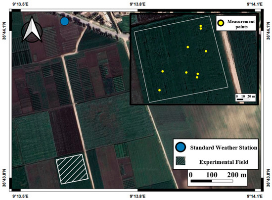
Figure 1.
Experimental field with the location of the standard meteorological station and measurement points; the zoom inserted in the top right corner shows the locations of the measurement of both gCC and SWC.
During the 2024–2025 cropping season, durum wheat (Triticum durum L., cv. Salim) was cultivated in a 100 m × 100 m (1 ha) experimental plot under rainfed conditions. Sowing took place on 12 December 2024 (defined as day 0) at a seeding density of 350 seeds m−2, and harvest was carried out on 15 June 2025 (185 Days After Sowing, hereinafter named DAS). Nitrogen fertilization was supplied as ammonium nitrate at a total rate of 150 kg N ha−1, applied in three splits corresponding to critical phenological stages: Z13 (three leaves unfolded, ≈25 DAS), Z16 (six leaves unfolded, ≈40 DAS), and Z32 (stem elongation, second node detectable, ≈75 DAS), according to the Zadoks scale. The field was also managed, with routine weed-control practices including a pre-emergence herbicide application and periodic field inspections that confirmed the absence of shrubs, perennial grasses, or other non-crop species throughout the season.
2.2. In Situ Data Collection
Meteorological data were obtained from a METOS® automated weather station (Pessl Instruments GmbH, Weiz, Austria) installed at the experimental site (Figure 1). Prior to analysis, the dataset was subjected to quality assurance and control (QA/QC), including detection and removal of outliers, logical consistency checks between variables, and verification of continuous records. The station recorded daily maximum and minimum temperatures, Tmax and Tmin (°C), precipitation, P (mm), relative air humidity, RH (%), wind speed at 2 m height a.g.l., U2 (m s−1), and global solar radiation, RS (MJ m−2 d−1). In this study, crop reference evapotranspiration, ETo, (mm d−1), was calculated using the FAO-56 Penman–Monteith (PM) equation [38] (Equation (1)), which is widely recognized as the most robust approach for estimating ETo across different climatic conditions [32,33]. The PM formulation assumes a hypothetical reference crop represented by a well-watered clipped grass surface with a uniform height of 0.12 m, a fixed surface resistance of 70 s m−1, and an albedo of 0.23 [30]:
where Rn is the surface net radiation (MJ m−2 d−1); G is the soil heat flux density (MJ m−2 d−1); Tmean is the mean daily air temperature (°C); U2 is the wind speed at a height of 2 m (m s−1); ea is the actual vapour pressure (kPa); es represents the saturation vapour pressure (kPa); ∆ is the slope of the saturation vapour pressure temperature curve (kPa °C−1), and γ is the psychrometric constant (kPa °C−1). Its accuracy in the Tunisian context has already been confirmed by Jabloun and Sahli [22], who demonstrated reliable performance when employed using downscaled climate input data.
Figure 2 shows the temporal dynamics of the main in situ meteorological variables used as input for the model implementation.
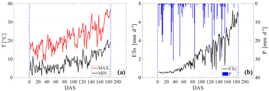
Figure 2.
Temporal dynamics of maximum (MAX) and minimum temperature (MIN) (a), and crop reference evapotranspiration (ETo) and precipitation depth (P) (b); the blue dashed lines indicate the sowing and the harvest.
Soil characterization was performed before sowing, with particle size distribution analyzed for three layers (0–20, 20–40, and 40–60 cm) using sieving and the Bouyoucos hydrometer method [5]. Soil hydraulic properties, including SWC at saturation, field capacity, and wilting point, were determined from soil water retention curves. Finally, saturated hydraulic conductivity was measured using the constant head method on undisturbed cores [39].
The soil texture was represented as a homogeneous clay loam profile (clay 34%, silt 40%, sand 26%). Hydraulic properties were derived from both field measurements and laboratory analyses using sieving for fractions > 74 μm and the Bouyoucos hydrometer method for finer particles. Soil hydraulic properties were determined from the soil water retention curve [4]. The values were consistent across horizons, with permanent wilting point (SWCwp) = 0.23 cm3/cm3 (−1500 kPa), field capacity (SWCfc) = 0.36 cm3/cm3 (−33 kPa), and saturation (SWCsat) = 0.50 cm3/cm3 (0 kPa). Saturated hydraulic conductivity (Ksat) was measured at 140 mm day−1 on undisturbed soil cores, corresponding to a total available water (TAW) of approximately 130 mm m−1 [40].
During the 2024–2025 season, SWC was monitored at a depth of 20 cm using a FieldScout TDR 350 probe (Spectrum Technologies Inc., Aurora, IL, USA). Measurements were conducted twice a week at nine randomly distributed GPS-referenced points across the 100 × 100 m rainfed durum wheat field (Figure 1). The site is flat and agronomically homogeneous, which ensured consistent conditions across the monitored area and allowed the sampling scheme to capture the temporal and spatial dynamics of soil moisture at 20 cm. The TDR 350 probe was previously calibrated to provide an accuracy of ±0.03 cm3 cm−3, thus ensuring reliable soil water content measures [41]. gCC was assessed at the same nine points every 15 days using the binary grid method [42], where a 1 × 1 m quadrat subdivided into 100 cells was placed horizontally above the wheat canopy, and each cell was evaluated by observing the canopy from above. A cell was classified as “covered” when ≥50% of its area was occupied by green or partially yellow-green foliage that still intercepted light [43]. To ensure a consistent delimitation of canopy dynamics, classification also considered foliage vitality, leaf posture, and light interception. Only turgid, upright, photosynthetically active leaves that formed part of the canopy surface were counted as cover, while senescent or collapsed tissues were excluded [18]. Because the 1 × 1 m quadrat was divided into ten cells per side, forming 100 equal squares of 0.01 m2 each, the number of squares classified as ‘covered’ directly represented the fraction of the canopy surface occupied by green foliage and, when expressed as a percentage, corresponded to the number of covered squares out of 100 [44]. Observations were conducted from crop emergence to full senescence [18]. Root development was also monitored near the same sampling locations, with root cores extracted and analyzed for length density and depth of maximum rooting intensity at the same frequency as the gCC observations, thereby enabling a parallel assessment of above- and below-ground growth dynamics [37]. At harvest, biological and grain yield were measured from 1 m2 quadrats at each sampling point, with above-ground biomass oven-dried at 70 °C to constant weight for biological yield determination, and grain yield obtained after threshing (expressed in tons per hectare) was used for evaluating AquaCrop simulations of biomass accumulation and final yield [4].
2.3. Remote Sensing Data
A database of high-resolution multispectral images (MSI) level 2A acquired by the Sentinel-2 twin satellites (2A and 2B) allowed systematic monitoring of the soil-vegetation system of the study area via time series of the Normalized Difference Vegetation Index (NDVI) [45], at a spatial resolution of 10 m and a temporal resolution of 5 days, approximately. NDVI was calculated as shown in Equation (2):
where ρnir and ρred are the near-infrared (Band 8; 785–899 nm) and red (Band 4; 650–680 nm) reflectance, respectively. A spatio-temporal matching filter developed under the Google Earth Engine (GEE) environment [46] allowed the selection of 14 cloud-free scenes over the study area during the 2024–2025 period. The analysis employed the “COPERNICUS/S2_SR_HARMONIZED” product. The “.filterDate()” function allowed excluding all images with a cloud cover percentage greater than 50% based on the “CLOUDY_PIXEL_PERCENTAGE” attribute. Finally, a visual inspection of the remaining scenes was then carried out to ensure the complete absence of clouds over the study area. Thus, the images were downloaded and pre-processed using the R (2024.04.2 Build 764 version) package toolbox “sen2r” [47]. Matlab® R2021b and QGIS version 3.4.3 were jointly used for the image pre-processing and for evaluating NDVI. As a result, a continuous time series of daily NDVI was obtained by employing linear interpolation between consecutive Sentinel-2 image pairs acquired at two different dates [48]. The average and standard deviation of NDVI were determined by considering only the pixels entirely contained inside the field perimeter (71 pixels).
Authors demonstrated that the gCC is correlated to vegetation indices with different functions [49]. As shown by Baret et al. [50], confirmed by Carlson and Ripley [51] and Gutman and Ignatov [52], there is a good relationship between the gCC and the NDVI. Buyantuyev et al. [53] estimated gCC from Landsat data by computing several vegetation indices. Among all the estimation methods, the linear mixture model has been widely applied [54,55,56,57,58,59,60,61,62].
Thus, gCC was derived from the NDVI time series (hereafter, named NDVI-gCC) using a linear relationship developed by Equation (3) [63]. This equation was adopted from a previously validated NDVI-gCC relationship developed for Mediterranean cereal systems [63]. Before its employment in this study, we verified its suitability using the measured-gCC observations collected in our field:
2.4. Reanalysis Data
Daily reanalysis data of maximum and minimum air temperature, Tmax and Tmin (°C), global solar radiation, RS (MJ m−2 d−1), dew-point temperature, Tdew (°C), and eastward and northward wind speed components measured at 10 m a.g.l., Uew and Unw (m s−1), were downloaded using the E5L Daily Aggregated–ECMWF Climate Reanalysis dataset, available in the GEE platform (ECMWF/ERA5-LAND/DAILY_AGGR, https://developers.google.com/earth-engine/datasets/catalog/ECMWF_ERA5_LAND_DAILY_AGGR, accessed on 7 July 2025).
The daily relative air humidity, RH (%), not available in the reanalysis database, was calculated as indicated in Equation (4) [38]:
where ea(Tdew) and es(T) are the actual and saturated vapour pressure corresponding to dew-point, Tdew, and actual air temperature, T, respectively.
Wind speed at 10 m a.g.l, U10 (m s−1), was calculated using the two components, Uew and Unw, according to the methodology proposed by Allen et al. [38]. Moreover, the daily wind speed at 2 m a.g.l., U2 (m s−1) was calculated based on the wind speed at the height 10 m a.g.l., U10 [m s−1], retrieved by the E5L database, assuming a logarithmic wind speed profile as presented in Equation (5) [38]:
The QA and QC of the E5L data were assessed through direct comparisons with numerous in situ observations, primarily collected between 2001 and 2018, as well as with other model-based or satellite-derived global reference datasets [30].
2.5. The AquaCrop Model
The AquaCrop model, developed by the FAO, is a water-driven decision-support tool designed to assist in scenario analysis and crop management planning. It integrates soil, crop, and atmospheric processes through a soil–water balance framework [19]. For each simulation, the model requires six main input datasets: (i) crop parameters, including phenological stages such as emergence, maximum gCC, onset of senescence, and maturity; (ii) soil physical and hydraulic properties; (iii) field management practices; (iv) irrigation scheduling; (v) initial soil water conditions; and (vi) climatic variables such as Tmax and Tmin, ET0, precipitation, and atmospheric CO2 concentration [64].
In this study, one of the main hypotheses to be validated was that E5L, when combined with Sentinel-2 canopy observations, could serve as a reliable alternative to the in situ data in the estimation of SWC dynamic and final biological and grain yield. To assess this hypothesis, we analyzed four simulation combinations, differing only in the source of meteorological forcing and gCC:
- -
- C1. In situ meteorological data and measured-gCC: All driving variables (Tmax, Tmin, Rs, RH, U2, and rainfall) were taken from the field station, and gCC was obtained from 1 × 1 m quadrat measurements. This configuration represents the reference (fully field-measured) case;
- -
- C2. E5L meteorological data and measured-gCC: The meteorological inputs were replaced by ERA5-Land data, while field-measured-gCC was retained. This isolates the effect of substituting station data with reanalysis forcing;
- -
- C3. In situ meteorological data and NDVI-gCC: The station meteorological dataset was preserved, but gCC was derived from the Sentinel-2 NDVI time series using Equation (3). This configuration evaluates the value of satellite-derived canopy cover compared to field measurements;
- -
- C4. E5L meteorological data and NDVI-gCC: Both meteorological and gCC inputs were derived from E5L and Sentinel-2, respectively. This represents the fully operational combination, in which no field measurements are required.
Comparisons among these combinations enabled assessing both the improvements obtained from assimilating Sentinel-2 information into AquaCrop and the potential of E5L to substitute for in situ meteorological forcing. The results were analyzed in terms of gCC, SWC, biological yield, and grain yield (the error statistics used to quantify deviations relative to in situ measurements are discussed in Section 2.6).
The initial condition of SWC was set according to the first measurement and was equal to 30.2%. The soil layer was automatically partitioned into compartments (5, 15, and 25 cm) for internal interpolation and water redistribution at initialization. The phenological calendar was defined from sowing (12 December 2024, DAS 0) to harvest (15 June 2025, DAS 185), for a total of 185 days. Crop development parameters differed between the combinations driven by measured-gCC (C1, C2) and NDVI-gCC (C3, C4). Phenological stages such as emergence, flowering, and maturity were parameterized based on in situ observations. The main calibrated parameters are summarized in Table 1.

Table 1.
Crop development parameters calibrated for durum wheat under different canopy cover inputs (measured-gCC; NDVI-gCC).
In addition to soil and canopy growth, production and evapotranspiration parameters were also calibrated for C1. Water productivity (WP) was set at 17 g m−2, consistent with values reported for durum wheat [65]. The crop coefficients for transpiration (KcTr) and for soil evaporation (Ke) were fixed at 1.20 and 1.10, respectively, in line with FAO-56 guidelines and previous AquaCrop applications [18]. Water productivity (WP) and harvest index (HI) were calibrated iteratively against C1 production, with WP and HI specifically adjusted to reproduce the biological biomass and grain yield. Rooting depth (Zr) was measured in the field. These parameters, together with KcTr, Ke, and cycle length, were kept constant across all four scenarios (C1–C4). Only the meteorological forcing (in situ vs. E5L) and gCC calibration source (measured-gCC vs. NDVI-gCC) varied among simulations. This ensured that differences among combinations were exclusively attributable to the source of meteorological input (in situ vs. E5L) and CC (measured-gCC vs. NDVI-gCC), while allowing fair comparisons under a consistent physiological basis for crop water use, biomass growth, and yield formation. The full set of calibrated, measured, fixed, and variable parameters used in the simulations is summarized in Table 2.
Table 2.
Summary of calibrated, measured, fixed, and variable parameters used in AquaCrop simulations.
2.6. Validations Metrics
To evaluate the performance of AquaCrop simulations and E5L meteorological data, statistical indices were calculated to quantify differences between observed and simulated values [66]. Statistical indices included the Root Mean Square Error (RMSE), Normalized RMSE (NRMSE), Mean Bias Error (MBE), Willmott’s index of agreement (d), determination coefficients with free intercept (R2), and Nash Sutcliffe Efficiency (NSE) (Table 3). These indices quantified meteorological data accuracy and the degree of agreement between simulated and observed SWC, gCC, biological yield, and grain yield. For these indices, ideal values correspond to RMSE, NRMSE, and MBE equal to 0, and d, R2, and NSE equal to 1, indicating perfect agreement between the observed and simulated data [4]. For SWC, in addition to these indices, a Taylor diagram [67] was employed to provide a synthetic evaluation of model performance. The Taylor diagram was applied to SWC because this variable is continuous and exhibits strong temporal dynamics, and its evaluation benefits from the simultaneous visualization of Standard Deviation (SD), Pearson correlation coefficient (R), and centred RMSE (RMSEc) [68]. This makes it well-suited for assessing how well AquaCrop simulations reproduce both the variability and the temporal coherence of measured SWC.
Table 3.
Performance metrics employed for AquaCrop calibration and E5L assessment.
In addition to the statistical indicators (Table 3), the reliability of E5L precipitation was evaluated using event-based indices (Table 4). Daily precipitation events were defined as days with precipitation greater than 0 mm. Three categorical indices were applied: Probability of Detection (POD), False Alarm Ratio (FAR), and Critical Success Index (CSI). POD measures the fraction of observed events that were correctly predicted, FAR quantifies the fraction of predicted events that did not occur, and CSI accounts for both missed and falsely predicted events, providing a balanced assessment of categorical skill [69]. These metrics were derived from a 2 × 2 contingency table, where a = hits (observed and predicted), b = misses (observed but not predicted), and c = false alarms (predicted but not observed) [70].
Table 4.
Categorical statistical indicators used for the evaluation of precipitation events.
3. Results
Section 3.1 shows the performance of E5L reanalysis compared with in situ observations for the assessment of Tmax and Tmin, precipitation, and ETo, which represent the key meteorological forcing inputs of the AquaCrop model. Subsequently, Section 3.2 investigates the reliability of NDVI-gCC to reproduce the temporal dynamics observed in field measurements. Thereafter, Section 3.3 details the calibration of AquaCrop canopy simulations using both measured-gCC and NDVI-gCC data. Finally, Section 3.4 analyses SWC and grain yield simulations obtained by applying the four input combinations.
3.1. Assessment of E5L Meteorological Inputs Using In Situ Observations
During the 2024–2025 wheat growth season, the capacity of E5L reanalysis data to reproduce in situ meteorological observations was evaluated for Tmax and Tmin, ET0, and precipitation using one-to-one scatterplots (Figure 3a–d) and statistical indices (Table 5). The one-to-one scatterplots (Figure 3a,b) illustrate that daily maximum (Tmax) and minimum (Tmin) temperatures were closely aligned with field data, with points clustering along the 1:1 line. ETo also exhibited a consistent linear relationship with in situ estimates, indicating a reliable representation of atmospheric evaporative demand by the reanalysis dataset. By contrast, precipitation displayed greater dispersion and a tendency toward underestimation, as evident from the points below the 1:1 line (Figure 3d). Despite this bias, rainfall occurrence and magnitude were captured with acceptable correspondence to observed events [71].
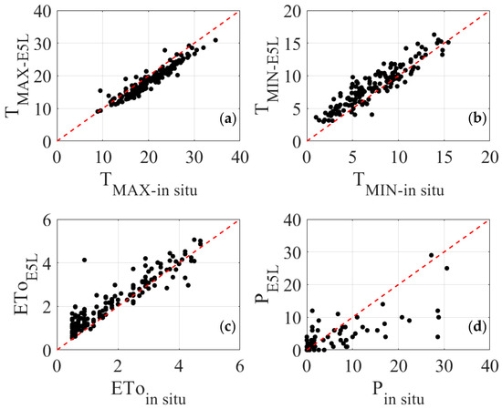
Figure 3.
Comparison between (a) daily maximum temperature, (b) daily minimum temperature, (c) daily crop reference evapotranspiration, and (d) daily precipitation depth registered by the standard weather station installed in the field and retrieved by the reanalysis data; the dashed red lines represent the 1:1 line (perfect match).
Table 5.
Statistical evaluation of meteorological variables from reanalysis against in situ measurements.
Statistical indices (Table 5) confirm these trends. E5L reproduced Tmax and Tmin with low RMSE (2.3 °C and 1.7 °C, respectively) and low NRMSE values (0.09 and 0.12), indicating good consistency with in situ measurements. The corresponding MBE values (−1.64 °C and +1.14 °C) suggest a slight systematic underestimation for Tmax and overestimation for Tmin. The high values of d (>0.93) and R2 (>0.84) confirmed the strong agreement and correlation between reanalysis and observed temperatures. ETo also aligned well with in situ observations, showing RMSE = 0.57 mm d−1, NRMSE = 0.14, MBE = +0.33 mm d−1, d = 0.94, R2 = 0.86, and NSE = 0.79, confirming its high reliability. In contrast, precipitation (P) presented greater dispersion around the 1:1 line, with RMSE = 4.14 mm d−1, NRMSE = 0.14, MBE = −0.96 mm, and lower agreement (d = 0.83, R2 = 0.62, NSE = 0.58), reflecting its larger spatial and temporal variability.
Event-based comparisons (Figure 4) further illustrated mismatches in rainfall detection, including missed and false rainfall events. Rainfall events were defined as any day with precipitation greater than 0 mm. POD, equal to 0.52, indicates that about half of the observed rainfall events were correctly identified by E5L, showing a moderate capability to capture rainfall occurrence. FAR, equal to 0.30, reveals that 30% of detected events did not actually occur, reflecting a moderate overestimation of event frequency. CSI, equal to 0.43, which integrates both missed and false events, confirms an adequate overall skill of E5L in reproducing the timing and frequency of rainfall events.
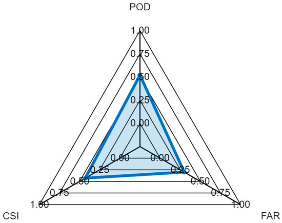
Figure 4.
Event-based verification of daily precipitation occurrence from E5L against in situ observations.
3.2. NDVI-gCC vs. Measured-gCC Comparison
Figure 5 illustrates the comparison between measured-gCC and NDVI-gCC throughout the growth cycle of durum wheat. Figure 5 shows that NDVI-gCC accurately reproduced the trend of canopy expansion during the early growth stages (DAS 26–71), even though some discrepancies between the observed and simulated values were present. However, at maximum canopy development (DAS 83–104), differences emerged both in terms of trend and magnitude. The maximum measured-gCC values were almost equal to 100%, while NDVI-gCC reached a maximum around 80%. During the first 20 days of senescence, NDVI-gCC decreased more slowly than measured-gCC. Between DAS 140 and 160, measured-gCC and NDVI-gCC values converged, as both methods captured the strong decline of the gCC.
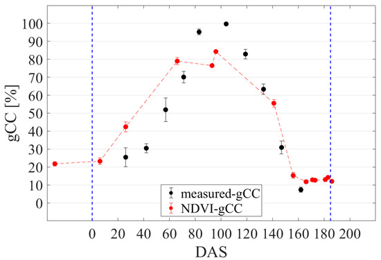
Figure 5.
Comparison of measured-gCC and NDVI-gCC dynamics; the blue dashed lines indicate the sowing and the harvest; error bars for measurements represent the standard deviation of the nine field measurement points.
Table 6 reports metrics employed to evaluate the fit between measured-gCC and the NDVI-gCC. The results indicated a good agreement between measured-gCC and NDVI-gCC, with RMSE = 15.65%, NRMSE = 0.27, d = 0.90, R2 = 0.78, and NSE = 0.73. The positive MBE (+3.09%) revealed a slight overestimation of NDVI-gCC compared to field measurements. Overall, these statistics confirm the suitability of NDVI-gCC to be used as the input of AquaCrop as it reproduced canopy development dynamics.
Table 6.
Statistical indicators comparing measured-gCC and NDVI-gCC during the 2024–2025 durum wheat growth cycle.
3.3. Assessment of AquaCrop Canopy Cover Simulations Under Calibration with Measured-gCC and NDVI-gCC
When calibrated with either measured-gCC or NDVI-gCC, AquaCrop reproduced the evolution of gCC dynamics during the 2024–2025 growth season (Figure 6). Both approaches captured canopy expansion and decline, but a closer correspondence was observed when using NDVI inputs. The simulation period started at DAS 26, corresponding to the first available observations after emergence, and ended at DAS 162–165, when canopy senescence was complete and harvest occurred. The slight variation in the crop cycle duration between both calibration methods (measured-gCC or NDVI-gCC) is mainly attributed to the differences in the canopy decline coefficient (CDC) used for the calibration of the gCC retrieval function (Table 1). The canopy decline coefficient (CDC) was 4.6% day−1 for the calibration based on measurements and 4.1% day−1 for NDVI-gCC, resulting in a slightly delayed decline phase in the NDVI-gCC simulations.
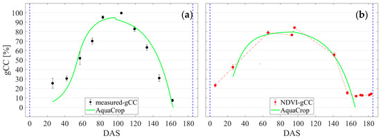
Figure 6.
Comparison of AquaCrop-simulated gCC vs. (a) measured-gCC and (b) NDVI-gCC; the blue dashed line indicates the sowing and the harvest timing; error bars for measurements represent the standard deviation of the nine field measurement points.
This was reflected in the statistical evaluation (Figure 7), where NDVI-derived calibration achieved lower error (RMSE = 5.29%) and higher efficiency (NSE = 0.93; d = 0.98), together with a slight stronger determination coefficient (R2 = 0.89), compared to field-based calibration (RMSE = 11.41%; NSE = 0.85; d = 0.96; R2 = 0.88). In general, statistical indicators highlighted a closer agreement between NDVI-gCC and AquaCrop simulations. This means that NDVI-gCC can accurately represent the temporal dynamics of wheat development, confirming that RS data can be reliably used to calibrate AquaCrop when field measurements are limited.
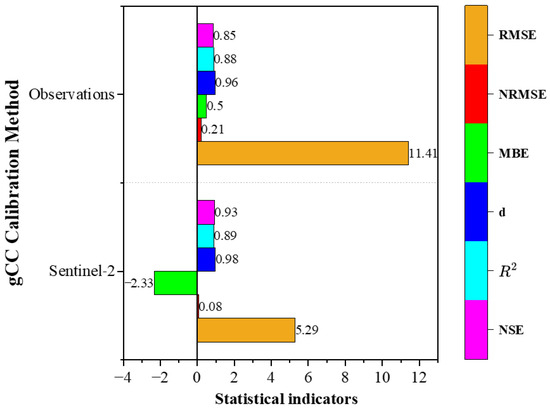
Figure 7.
Statistical evaluation of AquaCrop gCC simulations against measured-gCC (Observations) and NDVI-gCC (Sentinel-2) during the 2024–2025 growth season; the dashed line divides the statistics referred to Observations and Sentinel-2.
3.4. Assessing AquaCrop Simulations of Soil Water Content and Durum Wheat Yield Using the Different Input Combinations
The accuracy of AquaCrop in simulating the dynamics of SWC was evaluated for all the input combinations (Figure 8). The analysis of Figure 8C1–C4 shows that most discrepancies occur during the early and mid-season, when rainfall events and infiltration peaks drive rapid changes in SWC that AquaCrop tends to smooth. Late-season deviations are smaller because soil moisture becomes progressively dominated by evapotranspiration rather than rainfall inputs.
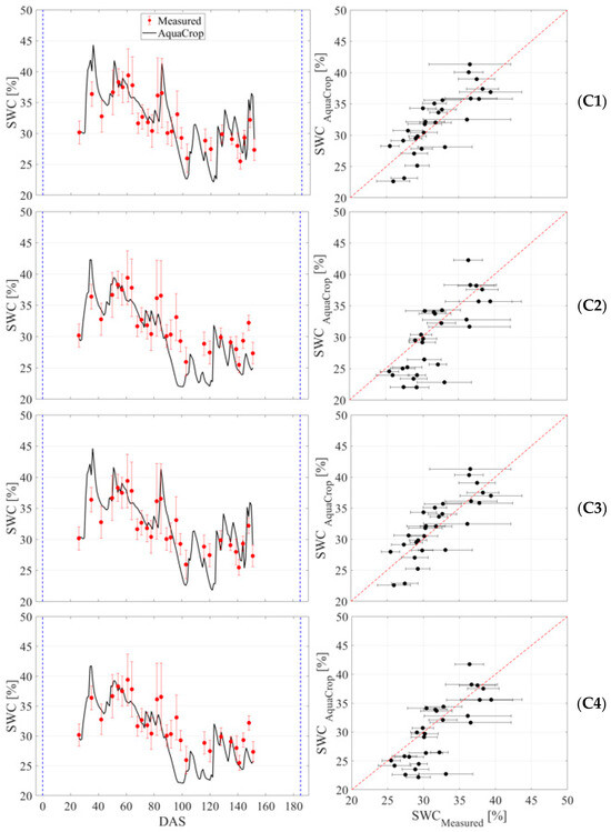
Figure 8.
Simulated (red dots with red standard deviation bars of the nine field measurements) and observed (black lines) soil water content (SWC) time series (left panels) and SWCmeasured vs. SWCAquaCrop scatterplots (right panels) under the four input combinations (C1–C4); (C1) in situ and measured-gCC; (C2) E5L and measured-gCC; (C3) in situ and NDVI-gCC; (C4) E5L and NDVI-gCC; the blue dashed lines on the time series indicate the sowing and the harvest timing, whereas on the right panels, the 1:1 (perfect match) is shown with dashed red lines.
Simulated and measured SWC exhibited a restricted reduction during the early growth stage (DAS 0–40) because of limited rooting depth and gCC (<10%). After that period, crop development accelerated, leading to an extension of the root systems and the improvement of canopy expansion, which increased crop transpiration. As a result, quick declines in SWC were observed, reaching a SWC of ~25%. During late growth (DAS 100–150), SWC reached 18–20%, reflecting the rise in atmospheric water demand, consistent with observations in semi-arid wheat systems [4]. To complement the graphical analysis, Table 7 reports the statistical indicators quantifying the model performance and revealing differences among the use of the four different input combinations. The lowest errors were achieved for C1 and C3 (RMSE = 2.73% and 2.72%, respectively; NRMSE = 0.09–0.08), indicating that simulations driven by in situ meteorological data reproduced SWC more accurately than those using E5L forcing. Combinations C2 and C4, which incorporated reanalysis inputs, showed slightly higher errors (RMSE was 3.96 and 3.82% for C2 and C4, respectively) and slightly larger NRMSE values (around 0.13). Configuration C1, using station meteorological data and measured-gCC, directly compares simulated SWC with in situ field observations, and therefore represents the field-based validation of AquaCrop in this study. For clarity and to avoid redundancy, the results achieved by employing the other combinations are validated considering C1 as a benchmark.
Table 7.
Statistical performance of AquaCrop simulations of SWC under the four input combinations.
The mean bias error (MBE) remained within ±2% for all combinations, confirming the absence of strong systematic bias. Willmott’s index of agreement (d) reached 0.89 for C1 and C3, compared with 0.82 for C2 and C4, confirming better correspondence between simulated and observed SWC when using in situ meteorological data. Similarly, the coefficient of determination (R2) was higher for C1 (0.67) and C3 (0.68) than for C2 and C4 (0.60), further highlighting the superior performance of simulations forced by station-based meteorology. NSE values were positive for all cases except C2 (−0.03), emphasizing that E5L-driven runs reproduce general SWC patterns but with lower efficiency.
The Taylor diagram (Figure 9) provides a complementary evaluation of model performance by jointly analyzing the R, SD, and RMSEc between simulated and observed SWC. Combinations C1 and C3 exhibited the highest correlations (R = 0.82 and 0.83, respectively) and the lowest RMSEc values (2.1% and 2.3%), with standard deviations (SD = 0.95–0.98) closely matching the observed variability. In contrast, C2 and C4 showed weaker correlations (R = 0.63 and 0.61) and higher RMSEc values (3.4% and 3.6%), together with slightly underestimated standard deviations (SD = 0.85–0.88).
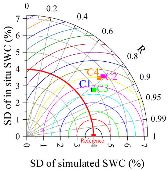
Figure 9.
Taylor diagram of AquaCrop SWC simulations under the four input combinations (C1–C4). The diagram presents the SD (%) and the Pearson correlation coefficient (R) of each simulation with respect to observations. The bold red semi-arc represents the scale of possible SD values, from low to high. The red square marks the observed SWC dataset and is placed on the arc at its SD (3.98%).
Yield prediction outcomes reflect the sensitivity of AquaCrop performance to different forcing data sources. Table 8 reports the observed Biological Yield (BY) and Grain Yield (GY), and the corresponding simulated values under the four input combinations. SDs are included for the observed data, serving as the reference against the variability from the mean value. Measured BY averaged 10.3 t ha−1 (±0.77) and GY 3.3 t ha−1 (±0.34). AquaCrop accurately reproduced both variables, with simulated yields remaining within the observed standard deviation range. The best agreement with field data was obtained for the combination using in situ meteorological inputs and measured-gCC, which reproduced BY and GY almost exactly (10.3 t ha−1 and 3.3 t ha−1, respectively). The use of E5L meteorological inputs led to a slight overestimation of yield (BY = 10.7 t ha−1, GY = 3.3 t ha−1), while the combination based on NDVI-gCC produced a slight underestimation (BY = 9.7 t ha−1, GY = 3.0 t ha−1). In general, the model performance remained consistent across combinations, confirming that the integration of Sentinel-2 canopy information can reliably support AquaCrop yield assessments when field measurements are not available.
Table 8.
Observed and simulated durum wheat biological yield (BY) and grain yield (GY) under the four input combinations (C1–C4); SDs are reported in parentheses.
4. Discussion
Application of crop water productivity models, like AquaCrop, requires a consistent description of the Soil–Plant–Atmosphere (SPA) continuum through simplified but process-oriented functions (e.g., soil water balance, canopy expansion, root development, and transpiration/evaporation partitioning) [72]. The better the parameterization of these processes, the higher the accuracy of the model in simulating crop responses to water [73]. Moreover, knowledge of soil and/or plant water status are crucial during model assessment, to evaluate its ability to reproduce SWC dynamics and vegetation development [74]. However, in many developing countries, continuous in situ measurements of SWC and gCC are rarely available [22,75]
The high spatial variability of precipitation, soil heterogeneity, and root distribution complicates the representativeness of point-based SWC probes, while field-based methods for gCC are labour-intensive and often fail to capture the non-linear trajectory of crop development. In these contexts, RS data offer a practical alternative [76]. Thus, vegetation indices, such as NDVI from Sentinel-2, provide spatially continuous descriptors of canopy dynamics. Instead, global reanalysis products such as E5L deliver spatially and temporally complete meteorological forcing where meteo-station networks are sparse or absent.
Experiments carried out during the 2024–2025 growth season allowed for evaluating AquaCrop under four meteorological (in situ or E5L data) and gCC parametrization (measured-gCC or NDVI-gCC) forcings. Accurate crop model simulations rely on robust meteorological forcing, making their evaluation against in situ observations a critical preliminary step [77]. In this study, E5L demonstrated strong agreement with in situ temperature data and ETo [30]; although, precipitation remained the most uncertain variable [78]. More locally, in Mediterranean conditions, E5L reproduced temperature with RMSE below 1 °C and NSE values above 0.8, confirming its suitability for agro-hydrological studies in semi-arid environments [28]. Despite the good agreement with in situ measurements, E5L exhibited systematic tendencies: slightly underestimating daily maximum and overestimating daily minimum temperatures. Such tendencies are already noted in the semi-arid regions of Iran [27]. Biases in temperatures could affect strongly crop modelling because a lower Tmax slows thermal time accumulation, potentially delaying phenological stages, while higher Tmin narrows the diurnal temperature range, influencing plant respiration and energy balance [79,80]. In the current study, the level of accuracy of E5L-derived ETo falls within the ranges reported for Southern Europe and North Africa (RMSE = 0.5–0.9 mm d−1), supporting the reliability of E5L for ETo estimation [68]. Nevertheless, findings from Fall et al. [80] in Senegal indicated that E5L and other reanalysis products diverged significantly from in situ data in capturing dry spell frequency and wet spell amplitude. In this context, the weaker performance of E5L for precipitation highlights the inherent difficulty of reproducing localized rainfall events in reanalysis datasets. Beck et al. [81] confirmed this limitation at the daily scale, showing that E5L underperforms compared to gauge–radar blended products when capturing localized storm dynamics. Likewise, a study from Spain showed that while E5L precipitation correlated moderately with observations (R ~ 0.5 up to 0.9 in rare cases), it consistently overestimated light–moderate precipitation and underestimated heavy events, especially along coastal areas and during summer [28]. Because precipitation controls soil water recharge, errors in rainfall propagate directly into the SWC, stress coefficient, and biomass formation, creating measurable differences in simulated crop growth. Huang et al. [71] quantified this effect as 10–14% biomass deviation under drought and wet conditions.
The comparison between measured-gCC and NDVI-gCC demonstrates the strong capacity of Sentinel-2 NDVI to capture the dynamics of durum wheat growth. The close agreement during canopy expansion highlights the robustness of NDVI in monitoring crop development stages, in line with findings reported for wheat and other cereals [63]. The statistical performance aligns with previous findings using Sentinel-2 imagery for canopy estimations in other crops, such as tomato, showing a regression coefficient almost equal to 1 (R2 = 0.99) and an RMSE of 11% [27]. At maximum canopy development, the underestimation of gCC primarily results from the saturation of reflectance-based indices when LAI exceeds 3–4, causing spectral responses to overlap and lose sensitivity [82,83,84]. This underestimation of gCC due to NDVI saturation propagates directly into AquaCrop, which relies on canopy cover to compute transpiration, biomass, and yield [80]. As a result, reduced NDVI sensitivity at high LAI leads AquaCrop to underestimate ETa and biomass production during peak canopy development [36]. This discrepancy also arises because the grid method classifies a cell as vegetation when at least half of its area is occupied by photosynthetically active canopy, including greenish canopy (early-senescent) leaves that remain physically present and continue intercepting light and transpiring [18]. In contrast, NDVI primarily reflects the spectral response of chlorophyll-rich tissues and thus underestimates gCC when non-green components become dominant [85]. During the early stages of senescence, NDVI declined more slowly than field observations, highlighting these methodological differences in sensitivity to canopy structural and physiological changes [86]. Between DAS 140 and 160, both methods captured the sharp decline of green biomass, and their estimates converged as senescent tissues lost optical influence on canopy reflectance, consistent with the reduction in photosynthetically active vegetation during late phenological stages [87]. Based on these results, Sentinel-2 NDVI provides a biophysically coherent input for the water balance model, enabling accurate simulation of green canopy evolution without the need for continuous measurements, and demonstrating the potential of RS data to support model calibration and validation under data-scarce conditions [88].
The graph of temporal SWC dynamics (Figure 8) highlights that AquaCrop simulations were able to reproduce the general trend of soil water content, with clear differences among the four input combinations. The Taylor diagram (Figure 9) shows that C1 and C3, as well as C2 and C4, cluster closely, reflecting their similar statistical behaviour. However, for station-driven combinations (C1 and C3), R reached values higher than 0.81, compared to 0.61 and 0.63 for C2 and C4, respectively. These results confirm that C1 and C3 provided a more accurate representation of the temporal dynamics of SWC than those driven by RS inputs. This finding is consistent with findings from a winter wheat study in Bekaa Valley of Lebanon, where integrating Sentinel-2 vegetation indices into AquaCrop improved the simulation of canopy cover, biomass, and yield under Mediterranean conditions [36]. The strong performance obtained when using NDVI-gCC confirms its reliability as an effective proxy for field-measured canopy data in AquaCrop simulations of SWC dynamics.
Statistical indicators (Table 3) not only confirm patterns observed in the Taylor diagram but also provide complementary insights into model behaviour by separating error magnitude (RMSE and NRMSE), systematic bias (MBE), efficiency in reproducing temporal variability (NSE), and overall agreement (R2 and d). When using in situ meteorological data as the model input, the RMSE values were the lowest (2.72–2.73%), NSE reached 0.51, and d was 0.89, indicating that AquaCrop reliably reproduced both the timing and amplitude of SWC dynamics [89]. The R2 of 0.67–0.68 further supported the agreement between the simulated and observed dynamics, consistent with previous calibration studies of AquaCrop for wheat [90]. The integration of Sentinel-2 gCC estimates with E5L reanalysis improved the ability of AquaCrop to simulate Crop Water Requirements (CWR) and yield [32]. Field evaluation on a tomato farm in Southern Italy showed that NDVI-gCC differed from measurement with an RMSE of about 11%, yet its assimilation improved the accuracy of both CWR and yield predictions [27]. In the current study, E5L-forced simulations exhibited an RMSE between 3.82 and 3.96%, negative or near-zero NSE values (–0.03 to 0.04), and a negative mean bias error (MBE = −1.67 to −1.78). These differences likely reflect the coarse spatial resolution of E5L data and its moderate ability to capture rainfall events (Figure 3d). These results indicate that the quality and representativeness of meteorological inputs exert a stronger influence on model performance than the source of canopy information and confirm that Sentinel-2 can provide a robust alternative to field canopy measurements when used together with in situ meteorological data.
AquaCrop reproduced durum wheat yields with the highest accuracy under in situ meteorological data with measured-gCC (C1: BY = 10.7 t ha−1, GY = 3.3 t ha−1), closely matching observations (10.3 ± 0.77 t ha−1; 3.3 ± 0.34 t ha−1) (Table 8). The lowest performance was obtained with E5L forcing and measured-gCC (C2: BY = 9.7 t ha−1, GY = 3.0 t ha−1), reflecting the influence of reanalysis biases on yield prediction. These results are consistent with recent studies that compared different modelling approaches for wheat yield estimation. Remotely sensed vegetation indices, particularly Sentinel-2 NDVI, have been shown to improve AquaCrop predictions by better constraining gCC development, a key driver of biomass and yield formation [91]. Proper calibration of canopy growth parameters (CGC, CDC, gCCx) using NDVI has been demonstrated to significantly reduce yield errors, which explains why the Sentinel-2 integration in our study (C3) produced more realistic estimates. At larger scales, however, reliance on reanalysis products such as E5L remains attractive due to their global coverage and operational availability. Previous studies confirm that although E5L introduces precipitation and temperature biases at the field scale, it can still provide sufficient skill for regional monitoring and forecasting when combined with RS datasets and soil databases such as soil grids [49,92]. This duality suggests that while station-based meteorology ensures the best yield accuracy at the farm level, the integration of E5L and RS data remains essential for scaling AquaCrop applications to regional or national food security assessments.
5. Conclusions
This study highlights the potential of integrating E5L reanalysis and Sentinel-2 satellite data into AquaCrop to enhance the simulation of durum wheat growth, SWC dynamics, and yields in semi-arid Tunisian conditions. Indeed, Tunisia, like other areas worldwide, suffers from a scarcity of in situ data; thus, the performance of the AquaCrop model using different levels of data availability were evaluated with the aim to demonstrate that the AquaCrop model could be extensively applied to other non-equipped fields to drive agriculture in these fragile areas. Across all performance indicators, the configurations using in situ meteorological data (C1 and C3) showed the highest accuracy, with the lowest SWC RMSE values (2.73% and 2.72%) and the highest R2 (0.67–0.68). Among the reanalysis-based configurations, C4 performed better than C2, showing lower SWC RMSE (3.82% vs. 3.96%) and similar R2 (both 0.60). C4 also produced realistic grain yield estimates (3.5 t ha−1), making it the most reliable option when field measurements are unavailable. However, the study is limited to a single site and one growing season, which constrains the generalization of outcomes. In addition, the calibration process focused on canopy and yield dynamics, without fully addressing other physiological processes. Model evaluation was also performed under the same field conditions due to the lack of independent datasets, which limits external validation. Future research should therefore extend to multiple sites and years and explore advanced data assimilation methods to improve model robustness under variable Mediterranean conditions. Moreover, uncertainties associated with Sentinel-2 canopy indicators (e.g., NDVI-gCC) and ERA5-Land meteorological forcing, such as retrieval noise, spatial aggregation effects, and errors in precipitation estimates may propagate into AquaCrop simulations and should be considered when interpreting the results. Further work should also explore advanced data-assimilation techniques and additional crop physiological parameters to enhance the predictive performance of AquaCrop under variable Mediterranean environments.
Author Contributions
Conceptualization, H.G., D.D.C. and M.I.; methodology H.G., D.D.C. and M.I.; software, H.G., D.D.C. and M.I.; formal analysis, H.G., D.D.C. and M.I.; investigation, H.G., D.D.C., M.I. and F.C.; resources, H.G.; data curation, H.G., D.D.C. and M.I.; writing—original draft preparation, H.G., D.D.C. and M.I.; writing—review and editing, H.G., F.C., D.D.C., M.I. and G.C.; visualization, H.G. and D.D.C.; supervision, G.C. and F.C. All authors have read and agreed to the published version of the manuscript.
Funding
This research received no external funding.
Data Availability Statement
The raw data supporting the conclusions of this article will be made available by the authors on request. However, some datasets are also free available: Daily ERA5-Land meteorological reanalysis data can be obtained from the Google Earth Engine platform (https://developers.google.com/earth-engine/datasets/catalog/ECMWF_ERA5_LAND_DAILY_AGGR, accessed on 7 July 2025), and Sentinel-2 images are available via Sentinel-HUB (https://browser.dataspace.copernicus.eu/, accessed on 14 June 2025).
Conflicts of Interest
Authors declare that the research was conducted in the absence of any commercial or financial relationships that could be construed as a potential conflict of interest.
Abbreviations
| List of acronyms: | |
| Acronym | Description |
| gCC | green Canopy Cover |
| SWC | Soil Water Content |
| E5L | ERA5-Land |
| NDVI | Normalized Difference Vegetation Index |
| NSE | Nash-Sutcliffe Efficiency Coefficient |
| RMSE | Root Mean Square Error |
| RMSEc SWB | Soil Water Balance |
| APSIM-Wheat | Agricultural Production Systems sIMulator-Wheat |
| CROPSYST | CROPping SYSTems |
| DSSAT-NWheat | Decision Support System for Agro-Technology-NWheat |
| STICS | Simulateur mulTIdisciplinaire pour les Cultures Standard |
| WOFOST | WOrld FOod STudies |
| FAO | Food and Agriculture Organization |
| ECMWF | European Centre for Medium-Range Weather Forecasts |
| DAS | Days After Sowing |
| QA | Quality Accuracy |
| QC | Quality Control |
| PM | Penman–Monteith |
| SWCwp | Soil Water Content at Wilting Point |
| SWCfc | Soil Water Content at Field Capacity |
| SWCsat | Soil Water Content at Saturation |
| TAW | Total Available Water |
| TDR | Time Domani Reflectometry |
| MSI | Multi Spectral Image |
| GEE | Google Earth Engine |
| gCC0 | green Canopy Cover initial |
| gCCx | green Canopy Cover maximum |
| CGC | Canopy Growth Coefficient |
| tCD | Canopy decline duration |
| CDC | Canopy Decline Coefficient |
| tFLOW | Flowering duration |
| tEM | Time to emergence |
| tCCx | Time to maximum canopy cover |
| tSen | Time to start of senescence |
| tMat | Time to maturity |
| WP | Water Productivity |
| HI | Harvest Index |
| MBE | Mean Bias Error |
| NRMSE | Normalized Root Mean Square Error |
| POD | Probability Of Detection |
| FAR | False Alarm Ratio |
| CSI | Critical Success Index |
| SD | Standard Deviation |
| BY | Biological Yield |
| GY | Grain Yield |
| List of symbols: | |
| Symbol | Description |
| Tmax and Tmin | minimum and maximum air temperature |
| P | precipitation |
| RH | relative air humidity |
| U2 | wind speed at 2 m above the soil |
| RS | global solar radiation |
| Rn | net radiation |
| G | soil heat flux |
| Tmean | mean air temperature |
| ea | actual vapour pressure |
| es | saturation vapour pressure |
| ∆ | slope of the saturation vapour pressure temperature curve |
| γ | psychrometric constant |
| ET0 | crop Reference Evapotranspiration |
| Ksat | saturated hydraulic conductivity |
| ρnir | near-infrared wavelength |
| ρred | red wavelength |
| Tdew | dew-point temperature |
| Uew | wind speed eastward component |
| Unw | wind speed northward component |
| U10 | wind speed at 10m above the soil |
| C1 | in situ meteorological data and gCC |
| C2 | E5L and measured-gCC |
| C3 | in situ meteorological data and NDVI-gCC |
| C4 | E5L and NDVI-gCC |
| Zr | root depth |
| KcTr | transpiration crop coefficient |
| Ke | soil evaporation crop coefficient |
| d | Willmott’s index |
| R2 | determination Coefficient |
| R | Pearson correlation coefficient |
References
- Rong, L.; Gong, K.; Duan, F.; Li, S.; Zhao, M.; He, J.; Zhou, W.; Yu, Q. Yield gap and resource utilization efficiency of three major food crops in the world—A review. J. Integr. Agric. 2021, 20, 349–362. [Google Scholar] [CrossRef]
- Van Vliet, M.T.H.; Thorslund, J.; Strokal, M.; Hofstra, N.; Flörke, M.; Macedo, H.E.; Nkwasa, A.; Tang, T.; Kaushal, S.S.; Kumar, R. Global river water quality under climate change and hydroclimatic extremes. Nat. Rev. Earth Environ. 2023, 4, 687–702. [Google Scholar] [CrossRef]
- Bönecke, E.; Breitsameter, L.; Brüggemann, N.; Chen, T.; Feike, T.; Kage, H.; Kersebaum, K.; Piepho, H.; Stützel, H. Decoupling of impact factors reveals the response of German winter wheat yields to climatic changes. Glob. Change Biol. 2020, 26, 3601–3626. [Google Scholar] [CrossRef]
- Ghazouani, H.; Jabnoun, R.; Harzallah, A.; Ibrahimi, K.; Amami, R.; Boughattas, I.; Milham, P.; Ghfar, A.A.; Provenzano, G.; Sher, F. Projected long-term climate change impacts on rainfed durum wheat production and sustainable adaptation strategies. J. Clean. Prod. 2025, 494, 144980. [Google Scholar] [CrossRef]
- Ghazouani, H.; Ibrahimi, K.; Amami, R.; Helaoui, S.; Boughattas, I.; Kanzari, S.; Milham, P.; Ansar, S.; Sher, F. Integrative effect of activated biochar to reduce water stress impact and enhance antioxidant capacity in crops. Sci. Total Environ. 2023, 905, 166950. [Google Scholar] [CrossRef] [PubMed]
- Sadok, W.; Schoppach, R.; Ghanem, M.E.; Zucca, C.; Sinclair, T.R. Wheat drought-tolerance to enhance food security in Tunisia, birthplace of the Arab Spring. Eur. J. Agron. 2019, 107, 1–9. [Google Scholar] [CrossRef]
- Bahri, H.; Annabi, M.; M’Hamed, H.C.; Frija, A. Assessing the long-term impact of conservation agriculture on wheat-based systems in Tunisia using APSIM simulations under a climate change context. Sci. Total Environ. 2019, 692, 1223–1233. [Google Scholar] [CrossRef]
- Holzkämper, A. Adapting agricultural production systems to climate change—what’s the use of models? Agriculture 2017, 7, 86. [Google Scholar] [CrossRef]
- Kersebaum, K.C.; Wallor, E. Process-based modelling of soil–crop interactions for site-specific decision support in crop management. In Precision Agriculture: Modelling; Springer: Cham, Switzerland, 2023; pp. 25–47. [Google Scholar]
- Peng, X.; Ren, J.; Chen, P.; Yang, L.; Luo, K.; Yuan, X.; Lin, P.; Fu, Z.; Li, Y.; Li, Y. Effects of soil physicochemical environment on the plasticity of root growth and land productivity in maize soybean relay strip intercropping system. J. Sci. Food Agric. 2024, 104, 3865–3882. [Google Scholar] [CrossRef] [PubMed]
- Zhang, Z.; Dobson, B.; Moustakis, Y.; Meili, N.; Mijic, A.; Butler, A.; Athanasios, P. Assessing the co-benefits of urban greening coupled with rainwater harvesting management under current and future climates across USA cities. Environ. Res. Lett. 2023, 18, 034036. [Google Scholar] [CrossRef]
- Hernández-Ochoa, I.M.; Gaiser, T.; Kersebaum, K.-C.; Webber, H.; Seidel, S.J.; Grahmann, K.; Ewert, F. Model-based design of crop diversification through new field arrangements in spatially heterogeneous landscapes. A review. Agron. Sustain. Dev. 2022, 42, 74. [Google Scholar] [CrossRef]
- Pequeno, D.N.L.; Ferreira, T.B.; Fernandes, J.M.C.; Singh, P.K.; Pavan, W.; Sonder, K.; Robertson, R.; Krupnik, T.J.; Erenstein, O.; Asseng, S. Production vulnerability to wheat blast disease under climate change. Nat. Clim. Change 2024, 14, 178–183. [Google Scholar] [CrossRef]
- Silva, J.M.P.; Bomio, M.R.D.; Motta, F.V.; Santos, R.M. Assessment of Calcimetry as a Reliable Method for Monitoring Soil Inorganic Carbon Stocks. ACS Agric. Sci. Technol. 2024, 4, 781–790. [Google Scholar] [CrossRef]
- Hall, R.J.; Wei, H.-L.; Pearson, S.; Ma, Y.; Fang, S.; Hanna, E. Complex systems modelling of UK winter wheat yield. Comput. Electron. Agric. 2023, 209, 107855. [Google Scholar] [CrossRef]
- Pasquel, D.; Roux, S.; Richetti, J.; Cammarano, D.; Tisseyre, B.; Taylor, J.A. A review of methods to evaluate crop model performance at multiple and changing spatial scales. Precis. Agric. 2022, 23, 1489–1513. [Google Scholar] [CrossRef]
- Huang, M.; Wang, C.; Qi, W.; Zhang, Z.; Xu, H. Modelling the integrated strategies of deficit irrigation, nitrogen fertilization, and biochar addition for winter wheat by AquaCrop based on a two-year field study. Field Crops Res. 2022, 282, 108510. [Google Scholar] [CrossRef]
- Raes, D.; Geerts, S.; Kipkorir, E.; Wellens, J.; Sahli, A. Simulation of yield decline as a result of water stress with a robust soil water balance model. Agric. Water Manag. 2006, 81, 335–357. [Google Scholar] [CrossRef]
- Iqbal, M.A.; Shen, Y.; Stricevic, R.; Pei, H.; Sun, H.; Amiri, E.; Penas, A.; del Rio, S. Evaluation of the FAO AquaCrop model for winter wheat on the North China Plain under deficit irrigation from field experiment to regional yield simulation. Agric. Water Manag. 2014, 135, 61–72. [Google Scholar] [CrossRef]
- Du, Y.; Fu, Q.; Ai, P.; Ma, Y.; Pan, Y. Modeling comprehensive deficit irrigation strategies for drip-irrigated cotton using AquaCrop. Agriculture 2024, 14, 1269. [Google Scholar] [CrossRef]
- Abdou, S.M.M.; Engel, B.A.; Emam, S.M.; El-Latif, K.M.A. AquaCrop Model Validation for Simulation Wheat Productivity under Water Stress Condition. Commun. Soil. Sci. Plant Anal. 2022, 53, 281–292. [Google Scholar] [CrossRef]
- Jabloun, M.; Sahli, A. Evaluation of FAO-56 methodology for estimating reference evapotranspiration using limited climatic data: Application to Tunisia. Agric. Water Manag. 2008, 95, 707–715. [Google Scholar] [CrossRef]
- Faniriantsoa, R.; Dinku, T. ADT: The automatic weather station data tool. Front. Clim. 2022, 4, 933543. [Google Scholar] [CrossRef]
- Lawal, I.M.; Bertram, D.; White, C.J.; Jagaba, A.H.; Hassan, I.; Shuaibu, A. Multi-criteria performance evaluation of gridded precipitation and temperature products in data-sparse regions. Atmosphere 2021, 12, 1597. [Google Scholar] [CrossRef]
- Sadeghi-Tehran, P.; Virlet, N.; Ampe, E.M.; Reyns, P.; Hawkesford, M.J. DeepCount: In-field automatic quantification of wheat spikes using simple linear iterative clustering and deep convolutional neural networks. Front. Plant Sci. 2019, 10, 1176. [Google Scholar] [CrossRef]
- Dlamini, L.; Crespo, O.; van Dam, J.; Kooistra, L. A global systematic review of improving crop model estimations by assimilating remote sensing data: Implications for small-scale agricultural systems. Remote Sens. 2023, 15, 4066. [Google Scholar] [CrossRef]
- Pelosi, A.; Belfiore, O.R.; D’Urso, G.; Chirico, G.B. Assessing Crop Water Requirement and Yield by Combining ERA5-Land Reanalysis Data with CM-SAF Satellite-Based Radiation Data and Sentinel-2 Satellite Imagery. Remote Sens. 2022, 14, 6233. [Google Scholar] [CrossRef]
- Gomis-Cebolla, J.; Rattayova, V.; Salazar-Galán, S.; Francés, F. Evaluation of ERA5 and ERA5-Land reanalysis precipitation datasets over Spain (1951–2020). Atmos. Res. 2023, 284, 106606. [Google Scholar] [CrossRef]
- Capecchi, V.; Pasi, F.; Gozzini, B.; Brandini, C. A convection-permitting and limited-area model hindcast driven by ERA5 data: Precipitation performances in Italy. Clim. Dyn. 2023, 61, 1411–1437. [Google Scholar] [CrossRef]
- Muñoz-Sabater, J.; Dutra, E.; Agustí-Panareda, A.; Albergel, C.; Arduini, G.; Balsamo, G.; Boussetta, S.; Choulga, M.; Harrigan, S.; Hersbach, H. ERA5-Land: A state-of-the-art global reanalysis dataset for land applications. Earth Syst. Sci. Data 2021, 13, 4349–4383. [Google Scholar] [CrossRef]
- Ippolito, M.; De Caro, D.; Cannarozzo, M.; Provenzano, G.; Ciraolo, G. Evaluation of daily crop reference evapotranspiration and sensitivity analysis of FAO Penman-Monteith equation using ERA5-Land reanalysis database in Sicily, Italy. Agric. Water Manag. 2024, 295, 108732. [Google Scholar] [CrossRef]
- Marta, A.D.; Chirico, G.B.; Bolognesi, S.F.; Mancini, M.; D’Urso, G.; Orlandini, S.; De Michele, C.; Altobelli, F. Integrating sentinel-2 imagery with Aquacrop for dynamic assessment of tomato water requirements in southern Italy. Agronomy 2019, 9, 404. [Google Scholar] [CrossRef]
- Ihuoma, S.O.; Madramootoo, C.A.; Kalacska, M. Integration of satellite imagery and in situ soil moisture data for estimating irrigation water requirements. Int. J. Appl. Earth Obs. Geoinf. 2021, 102, 102396. [Google Scholar] [CrossRef]
- Panek-Chwastyk, E.; Ozbilge, C.N.; Dąbrowska-Zielińska, K.; Wróblewski, K. Assessment of Grassland Biomass Prediction Using AquaCrop Model: Integrating Sentinel-2 Data and Ground Measurements in Wielkopolska and Podlasie Regions, Poland. Agriculture 2024, 14, 837. [Google Scholar] [CrossRef]
- Parida, B.R.; Kumar, A.; Ranjan, A.K. Crop types discrimination and yield prediction using sentinel-2 data and aquacrop model in Hazaribagh District, Jharkhand. KN-J. Cartogr. Geogr. Inf. 2023, 73, 77–89. [Google Scholar] [CrossRef]
- Saab, M.T.A.; El Alam, R.; Jomaa, I.; Skaf, S.; Fahed, S.; Albrizio, R.; Todorovic, M. Coupling remote sensing data and AquaCrop model for simulation of winter wheat growth under rainfed and irrigated conditions in a Mediterranean environment. Agronomy 2021, 11, 2265. [Google Scholar] [CrossRef]
- Cherif, I.; Kolintziki, E.; Alexandridis, T.K. Monitoring of land degradation in Greece and Tunisia using trends. Earth with a focus on cereal croplands. Remote Sens. 2023, 15, 1766. [Google Scholar] [CrossRef]
- Allen, R.G.; Pereira, L.S.; Raes, D.; Smith, M. FAO Irrigation and Drainage Paper No. 56; Food and Agriculture Organization of the United Nations: Rome, Italy, 1998; Volume 56, pp. 26–40. [Google Scholar]
- Amoozegar, A. Examination of models for determining saturated hydraulic conductivity by the constant head well permeameter method. Soil Tillage Res. 2020, 200, 104572. [Google Scholar] [CrossRef]
- Zhou, S.; Yu, B.; Lintner, B.R.; Findell, K.L.; Zhang, Y. Projected increase in global runoff dominated by land surface changes. Nat. Clim. Change 2023, 13, 442–449. [Google Scholar] [CrossRef]
- Noborio, K. Measurement of soil water content and electrical conductivity by time domain reflectometry: A review. Comput. Electron. Agric. 2001, 31, 213–237. [Google Scholar] [CrossRef]
- Verhegghen, A.; Kuzelova, K.; Syrris, V.; Eva, H.; Achard, F. Mapping canopy cover in african dry forests from the combined use of sentinel-1 and sentinel-2 data: Application to tanzania for the year 2018. Remote Sens. 2022, 14, 1522. [Google Scholar] [CrossRef]
- Mashonganyika, F.; Mugiyo, H.; Svotwa, E.; Kutywayo, D. Mapping of winter wheat using sentinel-2 NDVI data. a case of Mashonaland central province in Zimbabwe. Front. Clim. 2021, 3, 715837. [Google Scholar] [CrossRef]
- Douh, B.; Mguidiche, A.; Al-Marri, M.J.A.; Moussa, M.; Rjeb, H. Assessment of deficit irrigation impact on agronomic parameters and water use efficiency of six chickpea (Cicer arietinum L.) cultivars under Mediterranean semi-arid climate. Ital. J. Agrometeorol. 2021, 2, 29–42. [Google Scholar] [CrossRef]
- Rouse, J.W.R., Jr.; Haas, R.H.; Schell, J.A.; Deering, D.W. Paper a 20, in: Third Earth Resources Technology Satellite-1 Symposium. In Proceedings of the Symposium Held by Goddard Space Flight Center, Washington, DC, USA, 10–14 December 1973; p. 309. [Google Scholar]
- Gorelick, N.; Hancher, M.; Dixon, M.; Ilyushchenko, S.; Thau, D.; Moore, R. Google Earth Engine: Planetary-scale geospatial analysis for everyone. Remote Sens. Environ. 2017, 202, 18–27. [Google Scholar] [CrossRef]
- Ranghetti, L.; Boschetti, M.; Nutini, F.; Busetto, L. “sen2r”: An R toolbox for automatically downloading and preprocessing Sentinel-2 satellite data. Comput. Geosci. 2020, 139, 104473. [Google Scholar] [CrossRef]
- Pan, Z.; Hu, Y.; Cao, B. Construction of smooth daily remote sensing time series data: A higher spatiotemporal resolution perspective. Open Geospat. Data Softw. Stand. 2017, 2, 25. [Google Scholar] [CrossRef]
- Jiang, Z.; Huete, A.R.; Chen, J.; Chen, Y.; Li, J.; Yan, G.; Zhang, X. Analysis of NDVI and scaled difference vegetation index retrievals of vegetation fraction. Remote Sens. Environ. 2006, 101, 366–378. [Google Scholar] [CrossRef]
- Baret, F.; Clevers, J.G.P.W.; Steven, M.D. The Robustness of Canopy Gap Fraction Estimates from Red and Near-Infrared Reflectances: A Comparison of Approaches. Remote Sens. Environ. 1995, 54, 141–151. [Google Scholar] [CrossRef]
- Carlson, T.N.; Ripley, D.A. On the relation between NDVI, fractional vegetation cover, and leaf area index. Remote Sens. Environ. 1997, 62, 241–252. [Google Scholar] [CrossRef]
- Gutman, G.; Ignatov, A. The derivation of the green vegetation fraction from NOAA/AVHRR data for use in numerical weather prediction models. Int. J. Remote Sens. 1998, 19, 1533–1543. [Google Scholar] [CrossRef]
- Buyantuyev, A.; Wu, J.; Gries, C. Estimating vegetation cover in an urban environment based on Landsat ETM+ imagery: A case study in Phoenix, USA. Int. J. Remote Sens. 2007, 28, 269–291. [Google Scholar] [CrossRef]
- Zeng, X.; Dickinson, R.E.; Walker, A.; Shaikh, M.; DeFries, R.S.; Qi, J. Derivation and evaluation of global 1-km fractional vegetation cover data for land modeling. J. Appl. Meteorol. 2000, 39, 826–839. [Google Scholar] [CrossRef]
- Scanlon, T.M.; Albertson, J.D.; Caylor, K.K.; Williams, C.A. Determining land surface fractional cover from NDVI and rainfall time series for a savanna ecosystem. Remote Sens. Environ. 2002, 82, 376–388. [Google Scholar] [CrossRef]
- Montandon, L.M.; Small, E.E. The impact of soil reflectance on the quantification of the green vegetation fraction from NDVI. Remote Sens. Environ. 2008, 112, 1835–1845. [Google Scholar] [CrossRef]
- Delamater, P.L.; Messina, J.P.; Qi, J.; Cochrane, M.A. A hybrid visual estimation method for the collection of ground truth fractional coverage data in a humid tropical environment. Int. J. Appl. Earth Obs. Geoinf. 2012, 18, 504–514. [Google Scholar] [CrossRef]
- Yang, G.; Pu, R.; Zhang, J.; Zhao, C.; Feng, H.; Wang, J. Remote sensing of seasonal variability of fractional vegetation cover and its object-based spatial pattern analysis over mountain areas. ISPRS J. Photogramm. Remote Sens. 2013, 77, 79–93. [Google Scholar] [CrossRef]
- Zhang, X.; Liao, C.; Li, J.; Sun, Q. Fractional vegetation cover estimation in arid and semi-arid environments using HJ-1 satellite hyperspectral data. Int. J. Appl. Earth Obs. Geoinf. 2013, 21, 506–512. [Google Scholar] [CrossRef]
- Iordache, M.D.; Tits, L.; Bioucas-Dias, J.M.; Plaza, A.; Somers, B. A dynamic unmixing framework for plant production system monitoring. IEEE J. Sel. Top. Appl. Earth Obs. Remote Sens. 2014, 7, 2016–2034. [Google Scholar] [CrossRef]
- Guo, Z.; Shrestha, R.; Zhang, W.; Bhandary, P.; Yu, G.; Di, L. Land cover classification and change detection analysis using LandSat series and geospatial datasets in Nepal from 1980 to 2010. In Proceedings of the 2015 Fourth International-Conference on Agro-Geoinformatics (Agro-Geoinformatics), Istanbul, Turkey, 20–24 July 2015; pp. 414–418. [Google Scholar]
- Waldner, F.; Canto, G.S.; Defourny, P. Automated annual cropland mapping using knowledge-based temporal features. ISPRS J. Photogramm. Remote Sens. 2015, 110, 1–13. [Google Scholar] [CrossRef]
- Tenreiro, T.R.; García-Vila, M.; Gómez, J.A.; Jiménez-Berni, J.A.; Fereres, E. Using NDVI for the assessment of canopy cover in agricultural crops within modelling research. Comput. Electron. Agric. 2021, 182, 106038. [Google Scholar] [CrossRef]
- Wen, P.; Wei, Q.; Zheng, L.; Rui, Z.; Niu, M.; Gao, C.; Guan, X.; Wang, T.; Xiong, S. Adaptability of wheat to future climate change: Effects of sowing date and sowing rate on wheat yield in three wheat production regions in the North China Plain. Sci. Total Environ. 2023, 901, 165906. [Google Scholar] [CrossRef] [PubMed]
- Zhai, Y.; Huang, M.; Zhu, C.; Xu, H.; Zhang, Z. Evaluation and application of the AquaCrop model in simulating soil salinity and winter wheat yield under saline water irrigation. Agronomy 2022, 12, 2313. [Google Scholar] [CrossRef]
- Shirazi, S.Z.; Mei, X.; Liu, B.; Liu, Y. Assessment of the AquaCrop Model under different irrigation scenarios in the North China Plain. Agric. Water Manag. 2021, 257, 107120. [Google Scholar] [CrossRef]
- Taylor, K.E. Summarizing multiple aspects of model performance in a single diagram. J. Geophys. Res. Atmos. 2001, 106, 7183–7192. [Google Scholar] [CrossRef]
- Wadoux, A.M.-C.; Walvoort, D.J.J.; Brus, D.J. An integrated approach for the evaluation of quantitative soil maps through Taylor and solar diagrams. Geoderma 2022, 405, 115332. [Google Scholar] [CrossRef]
- Palharini, R.; Vila, D.; Rodrigues, D.; Palharini, R.; Mattos, E.; Undurraga, E. Analysis of extreme rainfall and natural disasters events using satellite precipitation products in different regions of Brazil. Atmosphere 2022, 13, 1680. [Google Scholar] [CrossRef]
- Bathelemy, R.; Brigode, P.; Boisson, D.; Tric, E. Rainfall in the Greater and Lesser Antilles: Performance of five gridded datasets on a daily timescale. J. Hydrol. Reg. Stud. 2022, 43, 101203. [Google Scholar] [CrossRef]
- Huang, X.; Ni, S.; Yu, C.; Hall, J.; Zorn, C.; Huang, X. Identifying precipitation uncertainty in crop modelling using Bayesian total error analysis. Eur. J. Agron. 2018, 101, 248–258. [Google Scholar] [CrossRef]
- Birhan, T.S.; Beyene, T.L.; Alemu, G.T.; Reta, B.G. Evaluation of the AquaCrop Model for Simulating Yield and Water Productivity of Maize (Zea mays L.) in Semi-Arid Ethiopia. Irrig. Drain. 2025. [Google Scholar] [CrossRef]
- Gavasso-Rita, Y.L.; Papalexiou, S.M.; Li, Y.; Elshorbagy, A.; Li, Z.; Schuster-Wallace, C. Crop models and their use in assessing crop production and food security: A review. Food Energy Secur. 2024, 13, e503. [Google Scholar] [CrossRef]
- Ghazouani, H.; Capodici, F.; Ciraolo, G.; Maltese, A.; Rallo, G.; Provenzano, G. Potential of thermal images and simulation models to assess water and salt stress: Application to potato crop in central Tunisia. Chem. Eng. Trans. 2017, 58, 709–714. [Google Scholar]
- Latrech, B.; Ghazouani, H.; Lasram, A.; M’hamdi, B.D.; Mansour, M.; Boujelben, A. Assessment of different methods for simulating actual evapotranspiration in a semi-arid environment. Ital. J. Agrometeorol. 2019, 2, 21–34. [Google Scholar]
- Xu, C.; Wang, W.; Hu, Y.; Liu, Y. Evaluation of ERA5, ERA5-Land, GLDAS-2.1, and GLEAM potential evapotranspiration data over mainland China. J. Hydrol. Reg. Stud. 2024, 51, 101651. [Google Scholar] [CrossRef]
- Wang, B.; Li, L.; Feng, P.; Chen, C.; Luo, J.-J.; Taschetto, A.S.; Harrison, M.T.; Liu, K.; Liu, D.L.; Yu, Q.; et al. Probabilistic analysis of drought impact on wheat yield and climate change implications. Weather. Clim. Extrem. 2024, 45, 100708. [Google Scholar] [CrossRef]
- Rahimikhoob, H.; Sohrabi, T.; Delshad, M. Variance-based global sensitivity analysis and uncertainty quantification of the AquaCrop model parameters for basil (Ocimum basilicum L.) under different nitrogen fertilizer rates. J. Plant Nutr. 2024, 47, 628–645. [Google Scholar] [CrossRef]
- Li, W.; Song, R.; Awais, M.; Ji, L.; Li, S.; Liu, M.; Lang, T.; Qi, H. Global sensitivity analysis of crop parameters based on AquaCrop Model. Water Resour. Manag. 2024, 38, 2039–2058. [Google Scholar] [CrossRef]
- Fall, C.M.N.; Lavaysse, C.; Drame, M.S.; Panthou, G.; Gaye, A.T. Wet and dry spells in Senegal: Comparison of detection based on satellite products, reanalysis, and in situ estimates. Nat. Hazards Earth Syst. Sci. 2021, 21, 1051–1069. [Google Scholar] [CrossRef]
- Beck, H.E.; Pan, M.; Roy, T.; Weedon, G.P.; Pappenberger, F.; Van Dijk, A.I.J.M.; Huffman, G.J.; Adler, R.F.; Wood, E.F. Daily evaluation of 26 precipitation datasets using Stage-IV gauge-radar data for the CONUS. Hydrol. Earth Syst. Sci. 2019, 23, 207–224. [Google Scholar] [CrossRef]
- Cui, T.; Sun, R.; Qiao, C.; Zhang, Q.; Yu, T.; Liu, G.; Liu, Z. Estimating diurnal courses of gross primary production for maize: A comparison of sun-induced chlorophyll fluorescence, light-use efficiency and process-based models. Remote Sens. 2017, 9, 1267. [Google Scholar] [CrossRef]
- Vannoppen, A.; Gobin, A. Estimating farm wheat yields from NDVI and meteorological data. Agronomy 2021, 11, 946. [Google Scholar] [CrossRef]
- Nguy-Robertson, A.; Gitelson, A.; Peng, Y.; Walter-Shea, E.; Leavitt, B.; Arkebauer, T. Continuous monitoring of crop reflectance, vegetation fraction, and identification of developmental stages using a four band radiometer. Agron. J. 2013, 105, 1769–1779. [Google Scholar] [CrossRef]
- Betlem, P.; Birchall, T.; Ogata, K.; Park, J.; Skurtveit, E.; Senger, K. Digital drill core models: Structure-from-motion as a tool for the characterisation, orientation, and digital archiving of drill core samples. Remote Sens. 2020, 12, 330. [Google Scholar] [CrossRef]
- Colombo, R.; Bellingeri, D.; Fasolini, D.; Marino, C.M. Retrieval of leaf area index in different vegetation types using high resolution satellite data. Remote Sens. Environ. 2003, 86, 120–131. [Google Scholar] [CrossRef]
- Dlamini, L.; Crespo, O.; van Dam, J.; Gaso, D.V.; de Wit, A. Estimating actual maize yield with WOFOST in data-scarce small-scale cropping systems of South Africa: Data assimilation approach. Int. J. Appl. Earth Obs. Geoinf. 2025, 144, 104848. [Google Scholar] [CrossRef]
- de Roos, S.; De Lannoy, G.J.M.; Raes, D. Performance analysis of regional AquaCrop (v6. 1) biomass and surface soil moisture simulations using satellite and in situ observations. Geosci. Model Dev. 2021, 14, 7309–7328. [Google Scholar] [CrossRef]
- Toumi, J.; Er-Raki, S.; Ezzahar, J.; Khabba, S.; Jarlan, L.; Chehbouni, A. Performance assessment of AquaCrop model for estimating evapotranspiration, soil water content and grain yield of winter wheat in Tensift Al Haouz (Morocco): Application to irrigation management. Agric. Water Manag. 2016, 163, 219–235. [Google Scholar] [CrossRef]
- Trombetta, A.; Iacobellis, V.; Tarantino, E.; Gentile, F. Calibration of the AquaCrop model for winter wheat using MODIS LAI images. Agric. Water Manag. 2016, 164, 304–316. [Google Scholar] [CrossRef]
- Tewes, A.; Hoffmann, H.; Nolte, M.; Krauss, G.; Schäfer, F.; Kerkhoff, C.; Gaiser, T. How do methods assimilating Sentinel-2-derived LAI combined with two different sources of soil input data affect the crop model-based estimation of wheat biomass at sub-field level? Remote Sens. 2020, 12, 925. [Google Scholar] [CrossRef]
- Bojanowski, J.S.; Sikora, S.; Musiał, J.P.; Woźniak, E.; Dąbrowska-Zielińska, K.; Slesiński, P.; Milewski, T.; Łączyński, A. Integration of Sentinel-3 and MODIS vegetation indices with ERA-5 agro-meteorological indicators for operational crop yield forecasting. Remote Sens. 2022, 14, 1238. [Google Scholar] [CrossRef]
Disclaimer/Publisher’s Note: The statements, opinions and data contained in all publications are solely those of the individual author(s) and contributor(s) and not of MDPI and/or the editor(s). MDPI and/or the editor(s) disclaim responsibility for any injury to people or property resulting from any ideas, methods, instructions or products referred to in the content. |
© 2025 by the authors. Licensee MDPI, Basel, Switzerland. This article is an open access article distributed under the terms and conditions of the Creative Commons Attribution (CC BY) license (https://creativecommons.org/licenses/by/4.0/).