Physically Consistent Runoff Simulation in Mountainous Catchments Using a Time-Varying Gated Hybrid XAJ–LSTM Model

Abstract

Accurate simulation of rainfall–runoff processes in mountainous catchments is essential for flood forecasting and water resource management. Traditional physically based models often suffer from structural rigidity and parameter uncertainty, while deep learning models, although effective in capturing nonlinear patterns, lack physical constraints and interpretability. To address these issues, this study developed a time-varying gated hybrid model (XAJ–LSTM) that integrates the Xinanjiang (XAJ) model with a Long Short-Term Memory (LSTM) network to improve runoff prediction accuracy and physical consistency. Hourly rainfall, temperature, potential evapotranspiration, and runoff data (2015–2023) from 17 small to medium mountainous catchments in Shi Yan and En Shi, Hubei Province, were used to drive and evaluate the XAJ, LSTM, and XAJ–LSTM models. The hybrid model achieved mean NSE and KGE values of 0.971 ± 0.020 and 0.962 ± 0.024, respectively, outperforming both individual models. In about 80% of the catchments, the gating parameter λ(t) showed a negative correlation with discharge, indicating adaptive adjustment between the physical and data-driven components. The coupled model reproduced both high- and low-flow processes well, with deviations in flow duration curves generally within ±5%. These findings demonstrate that the proposed time-varying gating structure effectively balances model accuracy, stability, and interpretability.

1. Introduction

Rainfall–runoff models are fundamental tools for understanding and managing water resources, supporting a wide range of decision-making processes such as flood regulation, reservoir operation, irrigation planning, drought mitigation, and ecosystem conservation [1,2,3,4]. Over the past decades [5,6], hydrological modeling has advanced significantly. Physically based process models, characterized by explicit process representation, high computational efficiency, and strong physical interpretability, have become essential tools in both scientific research and operational forecasting [7]. Among the physically based models developed in China [8], the Xinanjiang (XAJ) model is one of the most representative and widely applied [9]. It simulates the rainfall–runoff generation process within a physically interpretable framework, encompassing infiltration, evapotranspiration, and soil moisture dynamics [10]. With its concise structure, clear physical meaning, and relatively low data requirements, the model has been successfully applied in humid and semi-humid regions [11]. By adopting the “fill and spill” principle, the model conceptualizes the watershed as a series of interconnected soil storage units, effectively capturing the conversion of rainfall into runoff under natural conditions.

However, in mountainous small- and medium-sized catchments with complex terrain, rainfall exhibits high spatiotemporal variability, runoff pathways are diverse, and land surface conditions are heterogeneous, leading to highly nonlinear and time-varying runoff processes [12]. Traditional physically based models rely on empirical calibration and fixed structures. In mountainous catchments, their application is constrained by the availability of required data (e.g., soil type and depth) or by the simplified representation of processes, which limits parameter identifiability and regional transferability [13]. These challenges can be addressed by deep learning approaches, which do not require explicit input of difficult-to-obtain data types (e.g., soil data) and do not assume explicit physical processes, providing new technical pathways and research directions for runoff modeling in complex terrain and highly nonlinear catchments [14].

In recent years, Long Short-Term Memory networks (LSTM) [15] have shown significant potential in hydrological modeling [16,17]. LSTM can capture nonlinear temporal dependencies in time series data without requiring explicit assumptions about the underlying physical processes [18,19,20,21]. Its flexibility enables adaptation to diverse catchment conditions and hydrological scenarios, often outperforming traditional models in predictive accuracy [22,23,24]. Nevertheless, existing studies indicate that while purely physical models often suffer from structural rigidity and parameter uncertainty under complex terrain and highly nonlinear conditions, deep learning models, despite their predictive advantage, lack constraints to ensure mass conservation or process consistency [25].

Consequently, researchers have attempted to embed hydrological concepts within deep learning frameworks to establish correspondences between LSTM internal states and hydrological processes [26,27]. As research has progressed, hybrid modeling approaches that integrate physical mechanisms with deep learning have gradually emerged as an important direction in hydrological simulation. These models aim to combine the process constraints of physical models with the nonlinear learning capability of deep learning models, employing multi-level fusion strategies to achieve complementary strengths, thereby enhancing runoff prediction accuracy and physical interpretability [28].

Within this framework, various mechanism–learning coupling schemes have been proposed internationally. For example, Wang et al. (2024) introduced a physics-encoded deep learning framework for distributed hydrological modeling, demonstrating its advantages in spatial consistency and process preservation through an empirical study in the Amazon basin [29]; Höge et al. (2022) employed neural ordinary differential equations (Neural ODEs) to embed neural networks directly into conceptual model equations, enhancing predictive accuracy while maintaining structural interpretability [30]; Yu et al. (2024) developed a coupled framework of physical models and machine learning to improve runoff generation and volume prediction at the catchment scale [31]. He et al. (2024) proposed a physically constrained deep learning framework that unifies differentiable representation of physical equations with data-driven feature extraction at the watershed scale, substantially improving stability and interpretability during extreme runoff events [32]; Li et al. (2024) further developed a physics prior-constrained deep neural network (dNN), embedding energy and water balance processes within the network to improve runoff response simulation under climate change scenarios [33]; Xu et al. (2022) coupled a distributed hydrological model with deep learning in snow-dominated karst catchments, demonstrating that the hybrid framework effectively captures nonlinear hydrological responses while preserving physical consistency [34]; Zhu et al. (2025) calibrated model parameters using particle swarm optimization (PSO) and Bayesian optimization (BO), ensuring optimal model performance, with an LSTM module serving as a post-processing step to correct XAJ residuals and refine initial predictions to produce the final outputs [35]; Xu et al. (2024) used soil moisture outputs from a distributed hydrological model as deep learning inputs for monthly streamflow prediction, showing that hybrid inputs substantially improve prediction reliability and stability [36]; Liu et al. (2024) combined physical model outputs with LSTM at the national scale to enhance streamflow estimation accuracy [37]; Yang et al. (2024) integrated physical hydrological model outputs with interpretable machine learning in glacierized river basins to assess water balance [38]; Baghirov et al. (2025) applied a hybrid physical constraint and deep learning framework, using physical outputs as network inputs for water cycle simulation [39]. Collectively, these studies demonstrate that hybrid models can significantly improve generalization and process interpretability while maintaining physical consistency, providing a theoretical foundation for dynamic fusion and modeling. Among these diverse coupling frameworks, the “loosely coupled” approach, where physical model outputs serve as deep learning inputs, is particularly representative. This method feeds intermediate state variables from the physical model (e.g., effective rainfall, prior discharge, soil moisture) into the deep network, enhancing nonlinear representation and generalization while preserving physical consistency, thereby partially addressing the structural limitations of purely data-driven models.

Building on this, the present study draws inspiration from the dynamic weighting concept in deep learning [40,41] and extends it to hybrid hydrological–deep learning modeling. Specifically, we introduce a gating module as the core mechanism linking the physical model and the deep learning model. Unlike traditional fixed weighting, the gate weights are adaptively adjusted based on current hydrological states (e.g., effective rainfall, prior discharge) and model residuals, dynamically allocating contributions from the physical and deep learning branches. During flood peaks, the model automatically emphasizes the nonlinear response of the deep learning branch, while during baseflow periods, the physical process constraints are strengthened. Through this dynamic weighting mechanism, the hybrid model maintains stable predictive performance across different hydrological scenarios, effectively reducing biases of single models under complex conditions and significantly improving overall accuracy and physical consistency.

The main innovations and contributions of this study are as follows:

• A novel time-varying gated hybrid hydrological model (XAJ–LSTM) is developed, incorporating physically meaningful variables, including effective rainfall and prior discharge, into the LSTM network to enhance mass conservation and physical interpretability.
• Systematic validation across 17 mountainous small- and medium-sized catchments demonstrates that the proposed model significantly outperforms individual models in accuracy, stability, and cross-catchment generalization.

2. Study Area and Data

2.1. Study Area and Data Sources

To evaluate the applicability and interpretability of the proposed time-varying gated hybrid model (XAJ–LSTM) in complex mountainous catchments, this study selected 17 representative small- and medium-sized basins located in Shi Yan and En Shi, Hubei Province (Figure 1, Table 1). The catchment areas range from 37 to 792 km², covering typical mountainous headwater units. Both regions lie within the transitional zone between the second and third geomorphic steps of China and belong to the upper reaches of the Yangtze River Basin, associated with the Han River and Qing River systems, respectively. The study area is characterized by pronounced topographic relief, short flow paths, and highly nonlinear rainfall–runoff processes, representing typical mountainous hydrological conditions.

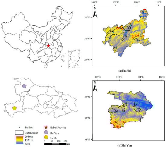
Figure 1. Distribution of 17 hydrological stations and small- to medium-sized catchments in the Shi Yan and En Shi regions.

Table 1. Basic characteristics of the 17 hydrological stations and their corresponding catchments in the Shi Yan and En Shi regions.

Prefecture	Station	River	Longitude (°E)	Latitude (°N)	Catchment Area (km2)
Shi Yan	Gu Shan	Guan Shan River	110.9278	32.4565	322
Shi Yan	Xian He	Xian He River	109.9005	32.3100	792
Shi Yan	Yan Ba	Zhu Xi River	109.8362	32.2832	598
Shi Yan	Ba Mudi	Shen Ding River	110.8143	32.7194	179
Shi Yan	Guan Fang	Xian River	109.7598	33.1094	296
Shi Yan	Hua Ligang	Jiang Jun River	110.3307	32.7083	371
Shi Yan	San Tai	Bei Xing River	110.2178	32.2913	420
En Shi	He Feng	Lou Shui River	110.0364	29.8919	649
En Shi	Shi Banping	Yandu River	110.3124	31.2495	466
En Shi	Li Chuan	Qing Jiang River	108.9003	30.2905	513
En Shi	Jian Shi chenguan	Guang Run River	109.7025	30.6023	151
En Shi	Zhong Lu	Yujiang River	108.7267	30.0146	452
En Shi	Long Fengba	Dai Shui River	109.4819	30.3737	434
En Shi	Da Miao	Yun Long River	109.2341	30.4899	153
En Shi	Jin Yinxi	Yun Long River	109.4696	30.1244	124
En Shi	Ding Zhai	Qu Jiang River	109.0402	29.5893	189
En Shi	San Kongqiao	Dong River	109.4946	30.2918	37

Shi Yan is situated on the southern foothills of the Qin–Daba Mountains in northwestern Hubei Province. The terrain is dominated by low and middle mountains and intermontane valleys, with deeply incised river valleys and steep slopes. The region experiences a subtropical monsoon climate, with a mean annual rainfall of approximately 1000–1200 mm. The main flood season occurs from June to September, characterized by intense and short-duration rainstorms that lead to rapid runoff responses and distinct “flash-rise and sharp-fall” hydrographs.

En Shi, located in the Wuling Mountains of southwestern Hubei Province, forms an important part of the upper Qing River Basin. The area exhibits highly dissected terrain with well-developed karst and structural landforms, where surface and subsurface runoff processes coexist. The mean annual precipitation generally exceeds 1600 mm, featuring high intensity, uneven spatial distribution, and frequent multi-peak runoff events, reflecting strong nonlinear hydrological responses.

Overall, both Shi Yan and En Shi are situated in the transitional zone between the second and third geomorphic steps of China, where terrain relief is significant, underlying surface conditions are complex, and rainfall exhibits strong spatiotemporal variability. This natural gradient provides an ideal experimental setting for assessing the applicability, robustness, and interpretability of the XAJ–LSTM model under different mountainous hydrological response conditions.

The hydro-meteorological datasets used in this study were obtained from the Hubei Provincial Bureau of Hydrology and Water Resources. The data cover the period 2015–2024 with an hourly temporal resolution. Meteorological variables include precipitation (P), evaporation (E), and air temperature (T), while the hydrological variable corresponds to the observed discharge (Q).

To incorporate physical constraints into the hybrid framework, the effective rainfall (P_e(XAJ₎) and prior discharge (Q₍XAJ₎) were independently simulated using the Xinanjiang (XAJ) model and subsequently used as additional input variables. These variables provide physically meaningful information that reflects the runoff generation and routing processes within the catchment.

Accordingly, the model input set in this study consists of precipitation, evaporation, air temperature, effective rainfall, and prior discharge, whereas the model output corresponds to the observed streamflow.

2.2. Data Preprocessing

To ensure data quality and the reliability of model training, a systematic preprocessing procedure was applied to the raw hydro-meteorological datasets. The main steps are summarized as follows:

• Data quality control and missing-value treatment

All meteorological and hydrological data were subjected to consistency checks to identify and remove abnormal values. Short-term missing data (less than 3 h) in precipitation, evaporation, and temperature series were filled using linear interpolation, while missing discharge values were replaced through temporal linear interpolation based on adjacent observations. Across the 17 catchments, missing records accounted for less than 1.5% of each time series, and periods with long-term data gaps were excluded from further analysis. Given the small proportion of missing data, the infilling procedure does not affect the subsequent model calibration and validation.

• Temporal resolution unification and synchronization

All hydro-meteorological variables were resampled to an hourly time step, and time stamps were aligned to ensure temporal consistency across datasets. For stations with different observation periods, only the overlapping period from 2015 to 2024 was retained to maintain completeness and temporal comparability of the samples.

• Calculation of effective rainfall and prior discharge

The effective rainfall ($P{e}_{\mathrm{XAJ}}$) and prior discharge ($Q_{\mathrm{XAJ}}$) for each catchment were independently simulated using the Xinanjiang (XAJ) model. The former reflects the regulation effect of the underlying surface on rainfall–runoff generation, while the latter captures the persistence and memory effects of hydrological processes. These two physically based variables were incorporated as additional inputs to the data-driven model, enhancing the physical interpretability of the hybrid framework.

• Normalization

To eliminate dimensional inconsistencies and accelerate model convergence, all input variables were normalized to the [0, 1] range using the Min–Max normalization method:

$$x^{\text{'}}={\displaystyle \frac{x-x_{\min }}{x_{\max }-x_{\min }}}$$

(1)

where $x$ is the original variable, $x_{\mathrm{m}\mathrm{i}\mathrm{n}}$ and $x_{\mathrm{m}\mathrm{a}\mathrm{x}}$ denote its minimum and maximum values over the training period, respectively, and $x^{\prime }$ is the normalized variable scaled to the range $[0,1]$.

This normalization procedure prevents gradient instability caused by differences in variable magnitudes.

• Dataset partitioning

For each catchment, the data were divided chronologically into training (70%) and validation (30%) subsets. The temporal split strategy avoids data leakage and ensures that the model’s generalization capability is evaluated on an independent time period.

After preprocessing, each catchment dataset comprised three input variables, namely, precipitation, evaporation, air temperature, and one output variable, the observed streamflow. These standardized datasets provided a consistent and physically meaningful basis for subsequent model training and performance evaluation.

3. Methodology

This study established three comparable runoff prediction schemes: a physically based model (XAJ), a deep learning model (LSTM), and a time-varying gated hybrid model (XAJ–LSTM). All experiments were conducted using hourly resolution data, with the datasets chronologically divided into training (70%) and validation (30%) subsets. Model performance was evaluated under a unified framework of assessment metrics.

3.1. Xinanjiang (XAJ) Model

The Xinanjiang (XAJ) model is a conceptual, process-based hydrological model founded on the principle of saturation-excess runoff generation. It simulates the hydrological processes of rainfall, infiltration, evapotranspiration, runoff generation, and flow routing to compute the catchment discharge.

In the XAJ model, the soil profile is conceptualized as three tension water storage layers—upper, middle, and lower zones—representing different soil moisture storages. In addition, a free-water reservoir is used to simulate the generation of various runoff components. The relationship between the runoff-producing area and the areal mean soil moisture storage (W) is expressed as:

$$F=1-{(1-{\displaystyle \frac{W}{WM}})}^{{\displaystyle \frac{B}{1+B}}}$$

(2)

where F is the fraction of the catchment producing runoff, W is the current areal mean soil moisture, WM is the maximum soil moisture capacity, and B is the spatial non-uniformity coefficient that controls the heterogeneity of soil moisture distribution.

In the XAJ model, runoff generation is represented using the three-source concept, in which the effective precipitation is partitioned into surface runoff, interflow, and groundwater flow according to the soil moisture storage conditions. The total effective rainfall contributing to the routing module is expressed as:

$$P_e = RS + RI + RG$$

(3)

where $P_e$ is the effective precipitation contributing to runoff generation (mm), $RS$ is the surface runoff component (mm), $RI$ is the interflow component generated from the soil moisture storage (mm), and $RG$ is the groundwater runoff component (mm).

After the effective precipitation is obtained, the XAJ model represents the temporal distribution of runoff response using the Nash unit hydrograph as:

$$UH(t)={\displaystyle \frac{t^{N-1}{e}^{-t/K}}{K^N\mathsf{\Gamma }(N)}}$$

(4)

where $UH\left(t\right)$ is the Nash unit hydrograph response at time $t$, $N$ is the shape parameter controlling the dispersion of the routing response, $K$ is the storage coefficient governing the time scale (h), and $\mathsf{\Gamma }\left(N\right)$ is the Gamma function.

After obtaining the effective precipitation, the XAJ model computes flow routing by convolving the effective rainfall with the Nash unit hydrograph. The routed discharge is expressed as:

$$Q(t)={\displaystyle \sum _{\tau =0}^t{P}_e(\tau )}UH(t-\tau )$$

(5)

where $Q\left(t\right)$ is the simulated discharge at time $t$, $P_e\left(\tau \right)$ is the effective precipitation at time $\tau$, and $UH\left(t-\tau \right)$ is the Nash unit hydrograph response for a unit rainfall pulse.

This convolution represents the integrated routing response of the catchment and forms the final runoff output of the XAJ model.

Model parameters were calibrated using an event-window optimization approach, minimizing the following objective function:

$$\min J=(1-NSE)+0.1\left|WBE\right|$$

(6)

where NSE denotes the Nash–Sutcliffe Efficiency, and WBE represents the water balance error percentage. The L-BFGS-B optimization algorithm was employed to efficiently identify the optimal parameter set within physically reasonable bounds.

After calibration, the model outputs the simulated discharge $Q_{XAJ}\left(t\right)$ and the effective rainfall $P_{e,XAJ}\left(t\right)$ for the entire study period. These two variables serve as physically based inputs for the subsequent coupled XAJ–LSTM model, providing process-level hydrological constraints to guide the data-driven learning component.

3.2. LSTM Model

The Long Short-Term Memory (LSTM) network is an improved form of the Recurrent Neural Network (RNN) capable of capturing long-term dependencies in time series data. Unlike conventional RNNs, the LSTM employs a gating mechanism—comprising an input gate, forget gate, and output gate—to dynamically regulate the transmission and updating of information, thereby avoiding the problem of gradient vanishing.

This characteristic makes the LSTM particularly suitable for modeling runoff processes, which exhibit pronounced temporal correlations and lagged responses. In runoff prediction, the LSTM typically takes meteorological forcing variables such as precipitation, evapotranspiration, and temperature as inputs, and outputs the streamflow $Q\left(t\right)$ at a future time step.

The core computational process of the LSTM can be expressed as follows:

$$f_t=\sigma (W_f\cdot [h_{t-1},x_t]+b_f)$$

(7)

$$i_t=\sigma (W_i\cdot [h_{t-1},x_t]+b_i)$$

(8)

$$o_t=\sigma (W_o\cdot [h_{t-1},x_t]+b_o)$$

(9)

$${\tilde{c}}_t=\tanh (W_c\cdot [h_{t-1},x_t]+b_c)$$

(10)

$$c_t=f_t\odot c_{t-1}+i_t\odot {\tilde{c}}_t$$

(11)

$$h_t=o_t\odot \tanh (c_t)$$

(12)

where $x_t$ is the input vector at time step $t$, $h_{t-1}$ and $c_{t-1}$ are the hidden state and cell state from the previous time step, respectively; $f_t$, $i_t$, and $o_t$ denote the forget, input, and output gates; ${\tilde{c}}_t$ is the candidate cell state; $c_t$ and $h_t$ are the updated cell state and hidden state at time $t$; $W_f$, $W_i$, $W_o$, and $W_c$ are the weight matrices, and $b_f$, $b_i$, $b_o$, and $b_c$ are the corresponding bias vectors. $\sigma (\cdot )$ is the sigmoid activation function, $\tanh \left(\cdot \right)$ is the hyperbolic tangent function, and ⊙ represents element-wise multiplication.

Through these gated operations, the LSTM can effectively extract latent temporal patterns from complex nonlinear systems.

In this study, the LSTM model takes multi-source hydro-meteorological variables—including precipitation, evaporation, air temperature, and antecedent hydrological states—as input features and outputs the streamflow at the next time step. The network adopts a sliding time-window structure with a window length of 72 h, enabling it to learn the dynamic evolution of the rainfall–runoff relationship from consecutive time sequences.

The LSTM architecture consists of two stacked LSTM layers, with 128 hidden units in the first layer and 64 hidden units in the second, followed by a fully connected output layer. The ReLU activation function is used [42], and the network is trained using the AdamW optimizer with an initial learning rate of 1 × 10⁻³ [43], batch size of 256, and 30 training epochs. The Mean Squared Error is adopted as the loss function.

Overall, the LSTM model effectively integrates meteorological forcing and antecedent catchment states to construct a nonlinear mapping of the rainfall–runoff relationship. It captures the temporal memory characteristics of the streamflow process and serves as a robust data-driven benchmark for performance comparison with the subsequent coupled model.

3.3. Time-Varying Gated XAJ–LSTM Coupled Model

To fully exploit the complementary advantages of the process-based hydrological model and the data-driven deep learning model, this study constructs a coupled runoff prediction framework based on a time-varying gating mechanism. The overall architecture of the model consists of three primary components (Figure 2):

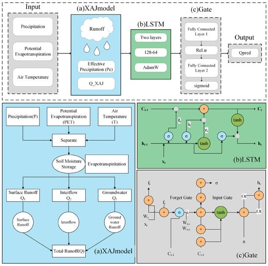
Figure 2. Schematic structure of the time-varying gated hybrid model (XAJ–LSTM).

• Process-based component (XAJ model):

The Xinanjiang (XAJ) model is based on the saturation-excess runoff generation principle, representing the physical processes of rainfall, infiltration, evapotranspiration, and flow routing. Its outputs, the simulated discharge $Q_{XAJ}\left(t\right)$ and effective rainfall $P_{e,XAJ}\left(t\right)$, describe the hydrological mechanisms of runoff generation and concentration. These physically consistent outputs are used as prior inputs to the subsequent deep learning network, ensuring that the coupled model remains constrained by hydrological principles.

• Data-driven component (LSTM network):

The LSTM network takes multiple hydro-meteorological features—including precipitation, evaporation, temperature, $Q_{XAJ}\left(t\right)$, the previous discharge $Q_{t-1}$, and $P_{e,XAJ}\left(t\right)$—as inputs to learn the complex nonlinear temporal mappings within the rainfall–runoff process. The LSTM output, $Q_{LSTM}\left(t\right)$, characterizes the model’s responsiveness to nonlinear and abrupt hydrological variations, showing advantages in capturing flood peaks and rapid flow transitions.

• Time-varying gating module:

The gating module serves as the core of the coupled model, determining at each time step $t$ the relative contributions of the process-based and data-driven components. It takes as inputs the current feature vector $x_t$, the LSTM hidden state $h_t$, and the outputs from the two branches, $Q_{XAJ}\left(t\right)$ and $Q_{LSTM}\left(t\right)$. Internally, the module applies a sequence of linear and nonlinear transformations to these multi-source inputs: the signals are first linearly combined and then passed through intermediate activation functions to enhance feature representation. Finally, the transformed information is mapped through a two-layer feed-forward fully connected network to produce the time-varying gating weight $\lambda \left(t\right):$

$$\lambda \left(t\right)=\sigma \left(W_2\mathrm{ReLU}\right(W_1\left[z_t\right]\left)\right),z_t=[x_t,h_t,Q_{XAJ}(t),Q_{LSTM}(t\left)\right]$$

(13)

where $z_t$ is the input feature vector of the gating network at time step $t$, composed of the current model input $x_t$, the LSTM hidden state $h_t$, and the outputs of the XAJ and LSTM branches, $Q_{XAJ}\left(t\right)$ and $Q_{LSTM}\left(t\right)$, respectively. $W_1$ and $W_2$ are the weight matrices of the first and second fully connected layers, ReLU(·) denotes the rectified linear unit activation function, and $\sigma (\cdot )$ is the sigmoid function that constrains the gating factor $\lambda \left(t\right)$ to the interval [0, 1]. The output $\lambda \left(t\right)$ represents the time-varying weight that adaptively balances the contributions of the XAJ and LSTM components.

$$Re{g}_{bimodal}=E\left[\lambda \right(t\left)\right(1-\lambda \left(t\right)\left)\right]$$

(14)

where $\lambda \left(t\right)$ is the time-varying gating factor at time step $t$, and $E[\cdot ]$ denotes the expectation operator computed over all time steps in the training sequence. The term $\lambda \left(t\right)(1-\lambda (t\left)\right)$ penalizes intermediate values of the gate and encourages the gating output to move toward the two endpoints (0 or 1), thereby promoting a more interpretable and bimodal gating behavior.

The total loss function used for training is defined as:

$$L_{total}=0.7(1-NSE)+0.3\left(MAE\right)+\beta Re{g}_{bimodal}$$

(15)

where $\beta ={10}^{-3}$ controls the regularization strength.

Analysis of the trained gating sequence $\lambda \left(t\right)$ reveals the dynamic dependency patterns between the two components under varying hydrological conditions: during high-flow or flood periods, $\lambda \left(t\right)$ tends to be smaller, indicating that the model relies more on the LSTM’s rapid-response capability; whereas during low-flow or baseflow conditions, $\lambda \left(t\right)$ increases, reflecting stronger reliance on the physically constrained XAJ branch.

This time-varying gating mechanism therefore provides the model with physical interpretability rather than functioning as a purely black-box weighted combination.

Unlike static hybridization schemes, the proposed coupled structure allows the model to automatically learn the optimal balance between physical and data-driven contributions during training. At each time step, the model autonomously determines whether to trust the process-based or neural component, achieving adaptive weighting across hydrological regimes. Compared with single models, the hybrid XAJ–LSTM architecture maintains physical consistency while enhancing its ability to represent the nonlinear dynamics of complex catchments.

Model training was performed using the AdamW optimizer with automatic mixed precision (AMP) to prevent gradient explosion and improve computational efficiency. During inference, the model simultaneously outputs the predicted discharge and the corresponding gating sequence, which can be further analyzed for interpretability. The final predictive output is expressed as:

$$\widehat{Q}(t)=\lambda (t)Q_{XAJ}(t)+[1-\lambda (t)]Q_{LSTM}(t),\lambda (t)\in [0, 1]$$

(16)

where $\widehat{Q}\left(t\right)$ represents the final predicted discharge from the coupled model, $Q_{XAJ}(t)$ is the output from the XAJ model, $Q_{LSTM}\left(t\right)$ is the output from the LSTM model, and $\lambda \left(t\right)$ denotes the time-varying gating factor.

3.4. Model Parameters and Evaluation Metrics

3.4.1. Model Parameters

To ensure model stability and comparability, all catchments were trained and validated under a unified parameter framework, as summarized in Table 2 and Table 3 The model inputs include precipitation, evaporation, air temperature, and discharge, which together provide the necessary hydro-meteorological information for the process-based, data-driven, and hybrid models.

Table 2. Parameter settings of the Xinanjiang (XAJ) model.

Symbol	Parameter Name	Initial Value	Range
WM	Maximum storage capacity (mm)	150	50–500
X	Upper soil water capacity coefficient (-)	0.40	0.05–0.90
Y	Lower soil water capacity coefficient (-)	0.50	0.05–0.95
B	Storage curve index (-)	0.30	0.05–1.50
KC	Evapotranspiration coefficient (-)	0.90	0.60–1.20
C	Soil moisture distribution coefficient (-)	0.05	0.00–0.20
IM	Impervious area ratio (-)	0.05	0.00–0.40
SM	Free water storage capacity (mm)	40	5–200
EX	Free water storage curve index (-)	1.20	0.20–3.00
KI	Interflow coefficient (-)	0.30	0.05–0.95
KG	Groundwater coefficient (-)	0.20	0.05–0.95
CI	Interflow recession constant (-)	0.95	0.50–0.999
CG	Groundwater recession constant (-)	0.995	0.90–0.9999
N	Nash unit hydrograph shape parameter (-)	2.50	1.00–6.00
K	Nash unit hydrograph time parameter (h)	18.0	2.00–60.0

Table 3. Hyperparameters of the LSTM model.

Parameter	Description	Value
Hidden units (Layer 1)	Number of hidden neurons in the first LSTM layer	128
Hidden units (Layer 2)	Number of hidden neurons in the second LSTM layer	64
Time window length	Length of input sequence (hours)	72
Activation function	Nonlinear activation used in fully connected layers	ReLU
Optimizer	Optimization algorithm	AdamW
Learning rate	Initial learning rate	1 × 10−3
Batch size	Number of samples per training batch	256
Training epochs	Total number of training iterations	30

In the XAJ model, parameters were calibrated using an event-window optimization method, in which the optimal parameter set was obtained by minimizing the objective function $(1-NSE)+0.1\left|WBE\right|$. The key parameters include runoff generation parameters $(W_M,X,B)$, evapotranspiration parameters $(K_C,C)$, free-water storage and groundwater recession coefficients $(K_I,K_G,C_I,C_G)$, and unit hydrograph shape parameters $(N,K)$. All parameters were constrained within physically reasonable ranges during calibration.

The LSTM model adopts a two-layer architecture, consisting of 128 hidden units in the first layer and 64 hidden units in the second layer, with a time window length of 72 h. The ReLU activation function was employed, and model optimization was performed using the AdamW algorithm with an initial learning rate of 1 × 10⁻³, a batch size of 256, and 30 training epochs.

In the coupled model, the time-varying gating network comprises two fully connected layers with 64 hidden units, utilizing a Sigmoid activation function to produce the gating weight $\lambda \left(t\right)$. A bimodal regularization term ($\beta ={10}^{-3}$) was incorporated to prevent the gating factor from converging toward the neutral mid-range, thereby enhancing the separability and interpretability of the gating dynamics.

3.4.2. Evaluation Metrics

To comprehensively evaluate the model performance, two widely used hydrological efficiency indicators were employed: the Nash–Sutcliffe Efficiency (NSE) and the Kling–Gupta Efficiency (KGE). Their formulations are presented as follows.

(1)

Nash–Sutcliffe Efficiency (NSE):

The NSE, proposed by Nash and Sutcliffe [44], measures the relative improvement of model simulations over the observed mean. It is defined as:

$$NSE=1-{\displaystyle \frac{\sum _{t=1}^N(Q_t^{sim}-Q_t^{obs}{)}^2}{\sum _{t=1}^N(Q_t^{obs}-{\bar{Q}}^{obs}{)}^2}}$$

(17)

where $Q_t^{obs}$ and $Q_t^{sim}$ denote the observed and simulated streamflow at time $t$, respectively, and ${\bar{Q}}^{obs}$ represents the mean of the observed discharge. An NSE value of 1.0 indicates perfect agreement between simulated and observed flows; 0.0 implies that the model performance is equivalent to using the observed mean as the predictor; while NSE < 0 suggests that the model performs worse than the mean benchmark.

(2)

Kling–Gupta Efficiency (KGE)

The KGE, proposed by Gupta et al. [45], decomposes the mean squared error into its correlation, variability, and bias components. It is calculated as:

$$KGE=1-\sqrt{{(r-1)}^2+{(\alpha -1)}^2+{(\beta -1)}^2}$$

(18)

where ris the Pearson correlation coefficient between simulated and observed discharge; $\mathsf{\alpha }={\displaystyle \frac{{\mathsf{\sigma }}_{\mathrm{s}\mathrm{i}\mathrm{m}}}{{\mathsf{\sigma }}_{\mathrm{o}\mathrm{b}\mathrm{s}}}}$ represents the variability ratio (agreement in flow variability); and $\mathsf{\beta }={\displaystyle \frac{{\mathsf{\mu }}_{\mathrm{s}\mathrm{i}\mathrm{m}}}{{\mathsf{\mu }}_{\mathrm{o}\mathrm{b}\mathrm{s}}}}$ represents the bias ratio (systematic deviation in mean flow). A KGE value closer to 1 indicates stronger consistency between simulated and observed series in terms of correlation, variability, and bias.

In this study, NSE and KGE were jointly used to evaluate the dynamic performance of the models across different catchments and hydrological scenarios. According to the empirical performance ratings proposed by Moriasi et al. [46], NSE or KGE values greater than 0.75 indicate excellent performance, values between 0.65 and 0.75 are good, and values below 0.50 are considered unsatisfactory.

(3)

Root Mean Square Error (RMSE)

The RMSE quantifies the overall deviation between simulated and observed discharge and is defined as:

$$RMSE=\sqrt{{\displaystyle \frac{1}{N}}{\displaystyle \sum _{t=1}^N{(Q_{sim,t}-Q_{obs,t})}^2}}$$

(19)

where $Q_{sim,t }$ is the simulated discharge at time $t$ (m³/s), $Q_{obs,t}$ is the observed discharge at time $t$ (m³/s), $N$ is the total number of time steps used for evaluation.

RMSE reflects the absolute magnitude of model prediction errors; smaller values indicate higher model accuracy and better overall fit.

(4)

Relative Bias (Bias)

The Bias evaluates the systematic deviation of simulated streamflow from observations in terms of overall water balance. It is defined as:

$$Bias(\%)={\displaystyle \frac{{\overline{Q}}_{sim}-{\overline{Q}}_{obs}}{{\overline{Q}}_{obs}}}\times 100\%$$

(20)

where ${\bar{Q}}_{sim}$ is the mean simulated discharge (m³/s), ${\bar{Q}}_{obs}$ is the mean observed discharge (m³/s).

Positive Bias values indicate overall overestimation of discharge, while negative values indicate underestimation. Models with |Bias| < 5% are classified as excellent, 5–10% as good, 10–15% as satisfactory, and >15% as unsatisfactory.

In summary, NSE and KGE assess the model’s ability to reproduce the temporal dynamics of streamflow, RMSE measures the absolute prediction accuracy, and Bias captures the degree of water balance error. Together, these metrics provide a comprehensive evaluation of model accuracy, stability, and physical consistency.

4. Results

4.1. Overall Performance Comparison of the Models

To systematically evaluate the simulation performance of the XAJ, LSTM, and XAJ–LSTM models, the runoff time series for each catchment was divided chronologically into a training period (70%) and an independent validation period (30%). All trainable components—including the conceptual parameters of the XAJ model, the weights and biases of the LSTM network, and the LSTM branch together with the gating module within the XAJ–LSTM framework—were calibrated exclusively on the training subset. The validation subset was not used during calibration and therefore provides an unbiased assessment of model skill under unseen hydrological conditions. Model performance was quantified using the NSE and KGE, and the calibration–validation results are summarized in Table 4.

Table 4. Comparison of the calibration and independent validation performance for the XAJ, LSTM, and XAJ–LSTM models across 17 mountainous catchments, based on the NSE and KGE.

Station/NSE	XAJ_cal	XAJ_val	LSTM_cal	LSTM_val	XAJLSTM_cal	XAJLSTM_val
Ba Mudi	−1.034	−0.242	0.144	0.327	0.914	0.936
Da Miao	0.402	0.440	0.834	0.861	0.978	0.982
Ding Zhai	0.041	0.072	0.908	0.506	0.977	0.950
Gu Shan	−0.206	−0.117	0.577	0.358	0.964	0.981
Guan Fang	0.128	−0.040	0.567	0.050	0.915	0.927
He Feng	0.543	0.664	0.659	0.748	0.966	0.961
Hua Ligang	−0.161	0.106	0.383	0.283	0.990	0.988
Jian Shichenguan	0.249	−0.402	0.751	0.748	0.987	0.975
Jin Yinxi	0.606	0.561	0.845	0.680	0.990	0.989
Li Chuan	0.667	0.689	0.901	0.842	0.998	0.999
Long Fengba	0.313	0.526	0.749	0.798	0.972	0.981
San Kongqiao	0.543	0.688	0.923	0.796	0.992	0.976
San Tai	−0.347	0.412	0.429	−0.019	0.991	0.949
Shi Banping	0.526	0.533	0.690	0.618	0.972	0.982
Xian He	0.180	0.485	0.677	0.394	0.911	0.983
Yan Ba	−0.387	0.553	0.653	0.495	0.986	0.986
Zhong Lu	0.114	0.586	0.878	0.430	0.974	0.968
Station/KGE	XAJ_cal	XAJ_val	LSTM_cal	LSTM_val	XAJLSTM_cal	XAJLSTM_val
Ba Mudi	0.194	0	0.118	0.308	0.939	0.928
Da Miao	0.386	0.380	0.787	0.881	0.989	0.984
Ding Zhai	0.145	0	0.925	0.470	0.977	0.91
Gu Shan	−0.036	0.156	0.563	0.367	0.950	0.963
Guan Fang	0.091	0	0.770	0.571	0.922	0.96
He Feng	0.598	0.580	0.817	0.774	0.954	0.932
Hua Ligang	0.410	0.542	0.392	0.292	0.980	0.990
Jian Shichenguan	0.433	0.379	0.665	0.774	0.990	0.984
Jin Yinxi	0.746	0.746	0.827	0.829	0.976	0.984
Li Chuan	0.774	0.667	0.948	0.885	0.998	0.998
Long Fengba	0.568	0.485	0.815	0.782	0.967	0.973
San Kongqiao	0.752	0.843	0.942	0.780	0.968	0.956
San Tai	0.208	0.136	0.359	0	0.985	0.938
Shi Banping	0.492	0.576	0.675	0.687	0.960	0.979
Xian He	0.382	0.570	0.707	0.277	0.938	0.966
Yan Ba	−0.017	0.776	0.829	0.422	0.968	0.962
Zhong Lu	0.541	0.54	0.935	0.326	0.984	0.953

Table 4 reveals pronounced differences among the three models across the two stages. The XAJ model exhibits moderate performance in both calibration and validation, with only limited improvement in the validation stage, reflecting the structural rigidity of conceptual process-based models. The standalone LSTM model achieves substantially higher NSE and KGE values during calibration; however, its performance deteriorates in several catchments during validation, indicating sensitivity to hydrological non-stationarity in the absence of explicit physical constraints. In contrast, the XAJ–LSTM model yields the highest and most stable performance across all catchments. Its calibration and validation efficiencies remain consistently high, and the smaller discrepancies between the two stages—as compared with the LSTM model—demonstrate the enhanced robustness and generalization capability introduced by the hybrid design.

To provide a more intuitive comparison, Figure 3 presents observed–simulated scatter plots for two representative catchments, San Kongqiao and Li Chuan, under the three modeling approaches. These two basins span contrasting hydrological regimes and therefore offer a stringent test of model transferability. The XAJ model displays large deviations from the 1:1 line, especially for high-flow events. The LSTM model exhibits a tighter point cloud but still underestimates certain flood peaks in the validation period. The XAJ–LSTM model shows the closest alignment with the 1:1 line in both basins and across both stages, and the high similarity between training and validation patterns indicates the absence of overfitting and strong predictive stability on independent samples.

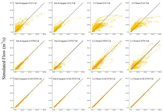
Figure 3. Observed–simulated scatter plots for two representative catchments (San Kongqiao and Li Chuan) under the XAJ, LSTM, and XAJ–LSTM models during the calibration and validation periods. The 1:1 reference line is shown to indicate the ideal agreement.

Figure 4 presents boxplots of NSE and KGE for the 17 catchments during the validation period. The XAJ model shows lower medians and wider interquartile ranges, revealing structural limitations in steep mountainous basins. The LSTM model improves overall accuracy but still exhibits considerable inter-catchment variability. The XAJ–LSTM model performs best in terms of both central tendency and dispersion, achieving the highest medians and the smallest interquartile ranges, and thus demonstrates superior spatial consistency and predictive stability across the region.

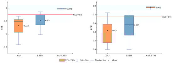
Figure 4. Overall performance comparison of the three models (XAJ, LSTM, and XAJ–LSTM) based on Nash–Sutcliffe efficiency (NSE) and Kling–Gupta efficiency (KGE) across 17 catchments.

Table 5 further summarizes the regional statistics for the validation period. The XAJ model yields the lowest mean efficiencies and the largest variability, while the LSTM model shows higher mean values but retains relatively large standard deviations. The XAJ–LSTM model achieves the highest mean NSE (0.971 ± 0.020) and mean KGE (0.962 ± 0.024), along with the smallest standard deviations, highlighting its strong balance between accuracy and robustness. Taken together, the calibration–validation comparison, representative station scatter plots, and regional performance statistics all confirm that the XAJ–LSTM model provides the most accurate and reliable streamflow simulations among the three approaches.

Table 5. Overall statistical performance of the three models based on NSE and KGE across 17 catchments.

Model	Mean NSE	Std. NSE	Mean KGE	Std. KGE
XAJ	0.324	0.351	0.434	0.280
LSTM	0.524	0.270	0.555	0.266
XAJ–LSTM	0.971	0.020	0.962	0.024

Overall, the three models can be ranked in terms of performance as XAJ–LSTM > LSTM > XAJ. Among them, the XAJ–LSTM model exhibits the best average accuracy, stability, and inter-catchment consistency, confirming the effectiveness of the coupling strategy in integrating physical constraints with data-driven learning. Unless otherwise stated, all subsequent performance analyses in this study are based solely on the independent validation period.

4.2. Spatial Distribution and Applicability of the Models

To investigate the differences in model performance under varying regional catchment conditions, the simulation results from 17 catchments in the Shi Yan and En Shi regions were analyzed through regional statistics and residual analysis (see Figure 5 and Figure 6, Table 6 and Table 7).

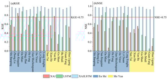
Figure 5. Regional comparison of model performance (XAJ, LSTM, and XAJ–LSTM) in the Shi Yan and En Shi catchments based on (a) KGE and (b) NSE.

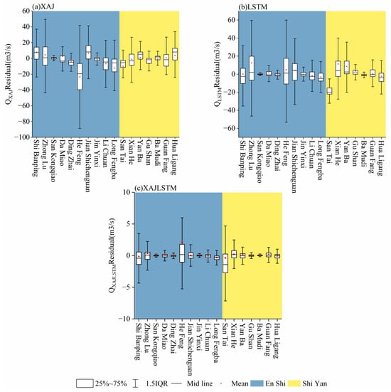
Figure 6. Spatial distribution of residuals for the three models (a) XAJ, (b) LSTM, and (c) XAJ–LSTM across 17 catchments in the Shi Yan and En Shi regions.

Table 6. Regional comparison of model performance (NSE and KGE) for XAJ, LSTM, and XAJ–LSTM in the Shi Yan and En Shi regions.

Region	Number of Catchments	NSE (XAJ)	NSE (LSTM)	NSE (XAJ–LSTM)
Shi Yan	7	0.165 ± 0.318	0.270 ± 0.187	0.964 ± 0.026
En Shi	10	0.408 ± 0.353	0.687 ± 0.144	0.974 ± 0.012
Region	Number of Catchments	KGE (XAJ)	KGE (LSTM)	KGE (XAJ–LSTM)
Shi Yan	7	0.311 ± 0.312	0.320 ± 0.174	0.958 ± 0.020
En Shi	10	0.503 ± 0.243	0.701 ± 0.183	0.962 ± 0.026

Table 7. Summary of residual statistics for the three models (XAJ, LSTM, and XAJ–LSTM), including mean range, standard deviation range, and overall residual range across 17 catchments.

Model	Mean Range (m3/s)	Std. Range (m3/s)	Overall Residual Range (m3/s)
XAJ	−4.07–7.99	12.4–30.4	−204–293
LSTM	0.12–12.43	9.5–38.1	−161–351
XAJ–LSTM	−0.15–0.33	0.78–9.41	−154–349

Figure 5 illustrates the distribution of NSE and KGE values across all catchments. Except for a few low-flow stations, the coupled XAJ–LSTM model exceeds the recommended performance threshold (NSE = 0.75, KGE = 0.75) in all catchments, demonstrating a consistently high level of accuracy. In contrast, the LSTM model still exhibits underestimation in several catchments (e.g., San Tai and Gu Shan), while the XAJ model shows NSE and KGE values below 0.5 for most basins, indicating limited adaptability to rapid changes in flow conditions.

As shown in Table 6, the performance of the individual XAJ and LSTM models varies across regions. In the Shi Yan area, the XAJ model achieved a mean NSE of only 0.165 ± 0.318, with negative values observed in some catchments, indicating that the purely physical model lacks the capability to capture nonlinear flood responses. The LSTM model performed better in this region, with the mean NSE increasing to 0.270 ± 0.187, although substantial variability remained. In contrast, overall simulation performance in the En Shi region was higher than that in Shi Yan. The LSTM model achieved a mean NSE of 0.687 ± 0.144 and a KGE of 0.701 ± 0.183, suggesting that the data-driven model performs more stably in humid catchments. The coupled XAJ–LSTM model, however, maintained consistently high accuracy in both regions, with mean NSE values of 0.964 in Shi Yan and 0.974 in En Shi, and corresponding KGE values of 0.958 and 0.962. The standard deviations were all below 0.03, indicating that the hybrid model exhibits excellent generalization ability and consistency across different catchment conditions.

To further analyze the error characteristics of the models across different regions, Table 7 summarizes the residual statistics of the three models for all 17 catchments. As shown in the table, the XAJ model exhibits the largest residual dispersion, with standard deviations ranging from 12 to 30 m³/s and peak errors reaching up to ±200 m³/s, indicating a typical tendency to underestimate flood peaks. Although the LSTM model shows overall improvement, it still presents noticeable bias under high-flow conditions, with maximum residuals exceeding 300 m³/s. In contrast, the residuals of the coupled XAJ–LSTM model are significantly more convergent, with standard deviations generally below 10 m³/s, mean residuals ranging from −0.15 to 0.33, and overall residuals constrained within ±150 m³/s, demonstrating a marked reduction in model error and enhanced stability.

As illustrated in the residual boxplots in Figure 6, the XAJ and LSTM models exhibit considerable variability in error distributions among different catchments, whereas the XAJ–LSTM model shows a markedly reduced box height, with the median and mean values nearly overlapping. This indicates that the coupled model with the time-varying gating structure can adaptively adjust the contributions of the physical and data-driven components under varying topographic and rainfall conditions, thereby substantially reducing the spatial dispersion of model errors.

In summary, the coupled model achieves both high accuracy and stability in the two regions, effectively eliminating the pronounced regional discrepancies observed between the standalone physical and data-driven models. The stable residual distribution and high consistency indices demonstrate that the gating mechanism effectively integrates physical constraints with nonlinear learning capability under diverse underlying surface conditions, providing a solid foundation for subsequent analyses of the gating parameters and hydrological processes.

4.3. Dynamic Characteristics of the Gating Parameter λ(t)

To gain a deeper understanding of the internal operating mechanism of the coupled model, it is necessary to analyze the dynamic behavior of the gating parameter λ(t), which serves as the core control variable of the XAJ–LSTM framework and governs the time-varying balance between the physical branch (XAJ) and the data-driven branch (LSTM). By examining the temporal evolution of λ(t) and its relationship with discharge (Q), the model’s adaptive weighting behavior under different hydrological conditions can be revealed, reflecting its ability to dynamically adjust between physical consistency and nonlinear learning. This analysis not only enhances the interpretability of the model but also verifies the effectiveness of the gating mechanism and reveals catchment-specific differences in hydrological responses. Typical results are shown in Figure 7 and Figure 8, and the corresponding statistical summaries are presented in Table 8 and Table 9.

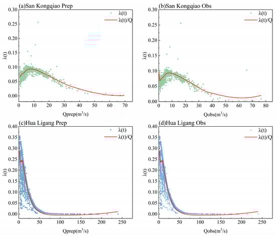
Figure 7. Relationship between the gating parameter λ(t) and discharge (Q) at two representative catchments: (a,b) San Kongqiao (non-significant response) and (c,d) Hua Ligang (significant response). The left panels show λ(t) versus predicted discharge (Q_pnep), and the right panels show λ(t) versus observed discharge (Q_obs).

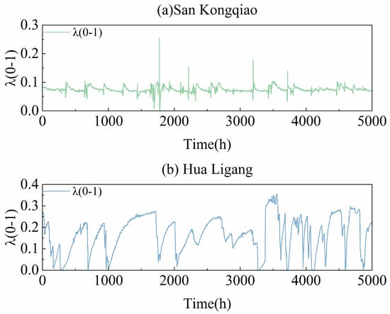
Figure 8. Temporal variations in the gating parameter λ(t) at two representative catchments: (a) San Kongqiao (non-significant response) and (b) Hua Ligang (significant response).

Table 8. Linear correlation statistics between the gating parameter λ(t) and discharge (Q) across all catchments.

Region	Station	R2	p-Value	Correlation Type	Significance	Regression Equation (λ = a + bQ)
Shi Yan	Ba Mudi	0.543	<0.001	Negative	✓ Significant	λ = 0.0812 − 0.00273 Q
Shi Yan	Hua Ligang	0.518	<0.001	Negative	✓ Significant	λ = 0.228 − 0.00322 Q
Shi Yan	Xian He	0.304	<0.001	Negative	✓ Significant	λ = 0.0552 − 0.000318 Q
Shi Yan	Yan Ba	0.273	<0.001	Negative	✓ Significant	λ = 0.0391 − 0.000206 Q
Shi Yan	Guan Fang	0.265	<0.001	Negative	✓ Significant	λ = 0.0795 − 0.00138 Q
Shi Yan	San Tai	0.258	<0.001	Negative	✓ Significant	λ = 0.296 − 0.00215 Q
Shi Yan	Gu Shan	0.0003	0.241	Negative	✗ Not significant	λ = 0.0974 − 0.000038 Q
En Shi	He Feng	0.251	<0.001	Negative	✓ Significant	λ = 0.0212 − 5.82 × 10−5 Q
En Shi	San Kongqiao	0.0006	0.075	Negative	✗ Not significant	λ = 0.0953 − 3.3 × 10−5 Q
En Shi	Shi Banping	0.171	<0.001	Negative	✓ Significant	λ = 0.0450 − 0.000378 Q
En Shi	Li Chuan	0.572	<0.001	Negative	✓ Significant	λ = 0.0394 − 0.000256 Q
En Shi	Jian Shichenguan	0.0395	<0.001	Negative	✓ Significant	λ = 0.0243 − 0.000165 Q
En Shi	Zhong Lu	0.326	<0.001	Negative	✓ Significant	λ = 0.0723 − 0.000322 Q
En Shi	Long Fengba	0.304	<0.001	Negative	✓ Significant	λ = 0.0393 − 0.000247 Q
En Shi	Da Miao	0.178	<0.001	Negative	✓ Significant	λ = 0.0293 − 0.000282 Q
En Shi	Jin Yinxi	0.202	<0.001	Positive	✓ Significant	λ = 0.1499 + 0.00194 Q
En Shi	Ding Zhai	0.135	<0.001	Negative	✓ Significant	λ = 0.0318 − 0.000362 Q

Table 9. Regional mean correlation statistics after removing outliers (R² < 0.05).

Region	Number of Stations	Mean R2 (Excluding Outliers)	Description
Shi Yan	6/7	0.36 ± 0.10	Strong linear negative correlation; highly dynamic gating response
En Shi	7/10	0.27 ± 0.12	Moderate negative correlation; relatively stable gating behavior
Overall	13/17	0.31 ± 0.11	Region-dependent adaptive gating patterns

As shown in Table 8, the gating parameter λ(t) exhibits a significant linear correlation with discharge (Q) in most catchments (p < 0.001), with R² values ranging from 0.17 to 0.57. Approximately 80% of the stations show a negative correlation, indicating that λ(t) decreases as discharge increases, while only Jin Yinxi station exhibit a positive correlation (R² = 0.20). The mean correlation coefficient across all catchments is R² = 0.31, suggesting a stable and consistent response between the gating parameter and the flow regime.

To further illustrate the overall pattern, Table 9 presents regional mean results after excluding low-explanatory stations (R² < 0.05). The overall mean R² is 0.31 ± 0.11, confirming a robust linear relationship between the model’s gating mechanism and variations in flow conditions. Combined with the results in Table 8 and Table 9, it can be concluded that the coupled model exhibits a stable negative correlation between λ(t) and Q in most catchments, with a mean R² of 0.31 ± 0.11. After removing outliers, the regional mean R² values for Shi Yan and En Shi are 0.36 ± 0.10 and 0.27 ± 0.12, respectively.

To further explore the differences and adaptive characteristics of the gating mechanism across catchments, two representative stations were selected for comparative analysis: Hua Ligang (significant-response type, R² = 0.52) and San Kongqiao (non-significant-response type, R² ≈ 0). This comparison aims to reveal the gating adjustment patterns of the model under different hydrological scenarios and to evaluate the physical rationality of the mechanism. Figure 7 illustrates the relationship between the gating parameter λ(t) and discharge (Q) for the two stations.

The results show that λ(t) at Hua Ligang exhibits a pronounced negative correlation with discharge. As flow increases, λ(t) decreases rapidly and approaches zero during high-flow periods. This behavior indicates that the model automatically strengthens the contribution of the data-driven branch (LSTM) during flood peaks to better capture complex nonlinear dynamics, while during low-flow conditions, λ(t) increases, emphasizing the physical branch (XAJ) to maintain mass balance and physical consistency. This pattern suggests that the gating mechanism adaptively allocates weights according to hydrological conditions and provides clear hydrological interpretability.

In contrast, the λ(t)–Q relationship at San Kongqiao shows no significant trend, with widely scattered points and a nearly flat fitted curve, indicating that the hydrological response in this catchment is relatively stable, and the gating adjustments are weak with nearly constant weighting. Overall, the response strength of λ(t) to discharge reflects the model’s adaptive capability and structural sensitivity under varying catchment conditions: in catchments with pronounced nonlinearity and sharp flood peaks, the gating mechanism demonstrates stronger dynamic adjustment and learning capacity, whereas in hydrologically stable basins, the model maintains a more balanced and consistent weight distribution.

The temporal variations in λ(t) are shown in Figure 8. At Hua Ligang, λ(t) exhibits clear periodic fluctuations over time, with a variation pattern largely synchronized with the discharge process. During the rising limb of flood events, λ(t) decreases rapidly and gradually recovers during the recession period, showing pronounced oscillations. This behavior indicates that the gating mechanism actively adjusts between the physical and data-driven branches under different flow conditions.

In contrast, the λ(t) curve at San Kongqiao is relatively smooth, showing only minor short-term decreases during several intense rainfall events, with overall fluctuations remaining small. This suggests that the gating mechanism in this catchment remains relatively stable, with limited dynamic adjustments. The differences between the two stations reflect the representative gating behaviors of significant- and non-significant-response catchments: the model exhibits stronger dynamic gating adjustments in highly responsive basins, whereas it maintains a more stable structure in weakly responsive ones.

The coupled model exhibits a stable negative correlation between λ(t) and discharge (Q) in most catchments, indicating that the gating mechanism adaptively adjusts the relative contributions of the physical and data-driven branches in response to changing flow conditions. This dynamic behavior enables the model to better capture rapid runoff generation and routing processes during flood peaks, while maintaining physical consistency and baseflow continuity during low-flow periods. Overall, the time-varying behavior of the gating parameter reflects the interpretability and structural robustness of the coupled model under diverse catchment conditions.

4.4. Runoff Simulation and Flow Duration Curves in Representative Catchments

To further evaluate the model performance in catchments with different gating-response types, two representative stations were selected for analysis: Hua Ligang (significant-response type) and San Kongqiao (non-significant-response type). All analyses were conducted based on the independent validation period to ensure the objectivity of model performance evaluation. The comparison focuses on the temporal evolution of streamflow and its statistical distribution (see Figure 9 and Figure 10, and Table 10). The hydrograph analysis reflects the model’s capability to reproduce dynamic hydrological responses during flood rising and recession stages, thereby assessing its ability to capture nonlinear runoff generation and routing processes. Meanwhile, the flow duration curve (FDC) analysis illustrates how well the model preserves flow variability and water balance across different flow regimes. By integrating these two perspectives, the analysis provides a comprehensive evaluation of the effectiveness and physical consistency of the gating mechanism under contrasting hydrological response conditions.

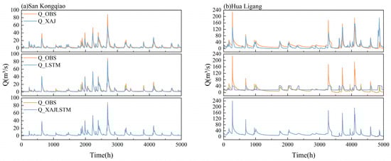
Figure 9. Comparison of simulated and observed hydrographs for the three models (XAJ, LSTM, and XAJ–LSTM) at two representative catchments: (a) San Kongqiao and (b) Hua Ligang.

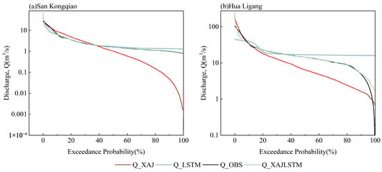
Figure 10. Comparison of flow duration curves between observed and simulated discharges for the three models (XAJ, LSTM, and XAJ–LSTM) at two representative catchments: (a) San Kongqiao and (b) Hua Ligang.

Table 10. FDC-based error metrics (RMSE and Bias) for the three models (XAJ, LSTM, and XAJ–LSTM) at two representative catchments: San Kongqiao and Hua Ligang.

Station	Model	RMSE	Bias (%)
San Kongqiao	XAJ	1.23	−3.14
San Kongqiao	LSTM	2.05	−6.25
San Kongqiao	XAJ–LSTM	1.68	−2.88
Hua Ligang	XAJ	8.43	−21.36
Hua Ligang	LSTM	11.02	−11.06
Hua Ligang	XAJ–LSTM	5.92	−1.16

As shown in Figure 9, the three models are generally able to capture the main fluctuations of the observed streamflow, although differences remain in peak magnitude, response timing, and low-flow performance.

At the Hua Ligang station, the XAJ model substantially underestimates most flood peaks, with both peak magnitude and timing deviating from the observations, indicating that the purely physical structure has limited responsiveness to rapid runoff generation processes. The LSTM model captures the overall flow variability but tends to underestimate peak flows in some high-flow periods and shows slight delays during recession phases. In contrast, the simulated hydrograph of the XAJ–LSTM coupled model closely aligns with the observed process, with markedly reduced errors in both peak timing and magnitude, while maintaining continuity and smoothness during low-flow periods. This suggests that the gating mechanism enables adaptive adjustment of the relative contributions of the physical and data-driven branches under varying flow conditions.

At the San Kongqiao station the overall flow process is relatively smooth, and differences among the three models are less pronounced. The XAJ model slightly underestimates discharge in several periods, whereas the LSTM model exhibits mild overestimation during a few rainfall events. The coupled model reproduces the observed hydrograph more consistently, effectively representing variations in medium and low flows. Overall, the coupled model demonstrates good temporal consistency in both types of catchments, with the degree of improvement being more evident in catchments characterized by stronger hydrological responses.

To quantitatively evaluate the models’ performance in reproducing flow distribution characteristics, flow duration curve (FDC) error metrics were calculated for two representative catchments, San Kongqiao and Hua Ligang (Table 10). At the San Kongqiao station, the XAJ–LSTM model achieved an RMSE of 1.68 and a Bias of −2.88%, outperforming both the XAJ model (RMSE = 1.23, Bias = −3.14%) and the LSTM model (RMSE = 2.05, Bias = −6.25%). The coupled model also exhibited more concentrated residuals and higher overlap between simulated and observed flow quantiles. At the Hua Ligang station, the FDC errors are more representative. The XAJ model showed significant underestimation in the high-flow range (Bias = −21.36%), while the LSTM model tended to overestimate low flows (Bias = +11.06%). In contrast, the XAJ–LSTM model achieved a Bias of −1.16% and an RMSE of 5.92, demonstrating balanced performance across both high- and low-flow conditions.

With the FDCs (Figure 10), the XAJ model exhibits systematic underestimation in the high-flow range, resulting in lower simulated flood peaks. The LSTM model, in contrast, shows a tendency to overestimate low flows, causing an upward shift in the baseflow portion of the curve. The XAJ–LSTM model, however, aligns closely with the observed curve across the entire range of flow quantiles, with deviations generally within ±5%. These findings are consistent with the RMSE and Bias results, indicating that the time-varying gating structure adaptively adjusts the relative contributions of the physical and data-driven branches in response to changing flow conditions. By maintaining overall water balance while improving the consistency of flow distribution, the coupled model demonstrates a synergistic effect between physical interpretability and nonlinear learning. Specifically, the model effectively avoids the peak underestimation typical of the physical model in the high-flow range and mitigates the drift observed in the data-driven model during low-flow periods, achieving robust adaptability across the full spectrum of flow conditions.

In summary, the results indicate that the XAJ–LSTM model achieves high simulation accuracy and structural stability in both significant- and non-significant-response catchments. In highly dynamic basins such as Hua Ligang, the gating mechanism enhances the nonlinear responsiveness of the LSTM branch, improving the reproduction of flood peaks. In weak-response basins such as San Kongqiao, the gating mechanism maintains balanced weighting between the two branches, preventing overfitting and oscillation. These findings are consistent with the λ(t)–Q analysis presented earlier, further confirming the coupled model’s adaptive capability under diverse hydrological regimes.

5. Discussion

This study systematically evaluated the runoff simulation performance of a physically based model (XAJ), a data-driven model (LSTM), and a gated hybrid model (XAJ–LSTM) across 17 small to medium mountainous catchments in Shi Yan and En Shi, Hubei Province, using hourly runoff data. The results show that the proposed XAJ–LSTM model outperformed both individual models in terms of accuracy, stability, and physical consistency. The mean NSE and KGE of the coupled model reached 0.971 ± 0.020 and 0.962 ± 0.024, respectively, exceeding those of the LSTM (NSE = 0.524 ± 0.270, KGE = 0.555 ± 0.266) and XAJ (NSE = 0.324 ± 0.351, KGE = 0.434 ± 0.280) models. Residual analysis further confirmed these findings: the residual ranges of the XAJ and LSTM models were relatively wide (−204–293 m³/s and −161–351 m³/s, respectively), whereas the errors of the XAJ–LSTM model were notably more convergent (−154–349 m³/s), with standard deviations generally below 10 m³/s and mean residuals ranging between −0.15 and 0.33. These results indicate that the coupled model maintained symmetric error distributions across different flow regimes, effectively avoiding the flood-peak underestimation and low-flow drift commonly observed in individual models.

At the regional scale, the coupled model exhibited highly consistent performance across both study areas. The mean NSE and KGE in the Shi Yan region were 0.964 ± 0.026 and 0.958 ± 0.020, respectively, while those in the En Shi region reached 0.974 ± 0.012 and 0.962 ± 0.026, with inter-regional differences below 0.02. In contrast, the XAJ and LSTM models showed stronger regional sensitivity, with standard deviations exceeding 0.18. These results demonstrate that the introduction of a time-varying gating structure significantly improved the adaptability and generalization capability of the model in steep, fast-responding, and highly nonlinear mountainous catchments.

From a structural perspective, the introduction of the gating parameter λ(t) not only enhanced the flexibility of the coupled model but also provided a foundation for its physical interpretability. As a dynamic variable that regulates the relative weighting between the physical branch (XAJ) and the data-driven branch (LSTM), variations in λ(t) directly reflect the system’s adjustment mechanism under different hydrological states. When λ(t) exhibits a significant correlation with discharge (Q), it indicates that the weighting adjustments are physically consistent with runoff generation and routing processes—decreasing during flood peaks to strengthen the data-driven branch and capture nonlinear, transient behaviors, and increasing during low-flow periods to reinforce physical constraints and maintain water balance and continuity. Moreover, the periodic fluctuations of λ(t) synchronized with the hydrograph reveal the coupling between internal model dynamics and external hydrological forcing. This λ(t)–Q–t mapping allows the internal model mechanism to be interpreted through observable variables. λ(t) can thus be regarded as a “dynamic feedback response function” of the system to nonlinear forcing, representing the model’s self-regulating behavior and achieving a unified link between data, process, and structure, thereby enhancing the model’s physical interpretability.

Based on this structural logic, the statistical characteristics of λ(t) and its relationship with flow regimes were analyzed to further elucidate the physical mechanisms behind the model’s improved performance. Results show that approximately 80% of the catchments exhibited a significant negative correlation between λ(t) and discharge (p < 0.001, R² = 0.17–0.57, mean R² = 0.31 ± 0.11). Among them, the Hua Ligang station demonstrated the strongest response (R² = 0.52), while the San Kongqiao station showed a nearly neutral relationship (R² ≈ 0). Notably, Jin Yinxi is the only catchment exhibiting a positive correlation. This behavior can be attributed to its hydrological and geomorphic characteristics—moderate terrain slopes, a high proportion of groundwater contributions, and relatively subdued flood peaks—which allow the XAJ branch to perform more reliably under medium-to-high flow conditions, resulting in a slight increase in λ(t) with rising discharge. In strongly responsive catchments, λ(t) decreased rapidly with increasing discharge and gradually recovered during the recession period, forming periodic oscillations synchronized with the hydrograph. This behavior indicates that λ(t), as an internal adaptive regulator, reflects the intensity of hydrological nonlinearity: during flood events, λ(t) decreases to enhance the contribution of the LSTM branch, while during recession or stable flow conditions, λ(t) increases to strengthen the physically constrained XAJ branch, thereby dynamically balancing physical consistency and nonlinear learning across different flow regimes.

Comparative analyses between significant- and non-significant-response catchments further validated the above mechanism. At the Hua Ligang station (a significant-response catchment), the XAJ model underestimated flood peaks and showed delayed responses, whereas the LSTM model captured overall trends but underestimated peak magnitudes. The XAJ–LSTM model accurately reproduced both the timing and magnitude of flood peaks, reflecting effective coordination between the physical and data-driven branches. At the San Kongqiao station (a non-significant-response catchment), the differences among the three models were smaller, and the coupled model exhibited lower residuals and greater stability during medium- and low-flow conditions. The flow duration curve (FDC) analysis yielded consistent results: at San Kongqiao, the XAJ–LSTM model achieved RMSE = 1.68 and Bias = −2.88%, outperforming XAJ (RMSE = 1.23, Bias = −3.14%) and LSTM (RMSE = 2.05, Bias = −6.25%); at Hua Ligang, the coupled model (RMSE = 5.92, Bias = −1.16%) substantially reduced the high-flow underestimation of the XAJ model (Bias = −21.36%) and the low-flow overestimation of the LSTM model (Bias = +11.06%). Overall, the XAJ–LSTM model maintained deviations within ±5% across the full flow percentile range, with simulated curves closely matching the observations.

Overall, the XAJ–LSTM model achieves a unified representation of simulation accuracy and physical interpretability in complex mountainous catchments. Through the time-varying gating mechanism, the model not only improves flood-peak representation and low-flow stability but also enhances inter-catchment consistency. The significant λ–Q correlations and reduced regional variance confirm that the adaptive gating structure enables robust performance under diverse hydrological conditions. Future work should extend this framework toward spatially distributed gating designs, incorporate multi-source hydro-meteorological inputs, and evaluate its performance under non-stationary climate scenarios, with the aim of developing hybrid hydrological models that are both physically transparent and robust across scales and climatic regimes.

6. Conclusions

This study developed and evaluated a time-varying gated hybrid model (XAJ–LSTM) that integrates the physically based Xinanjiang (XAJ) model with a Long Short-Term Memory (LSTM) network to improve runoff simulation in complex mountainous catchments. Using hourly runoff data from 17 small to medium catchments in Shi Yan and En Shi, Hubei Province, the model’s performance was systematically compared in terms of accuracy, stability, and physical consistency.

The results show that the XAJ–LSTM model performs better than the individual models in terms of simulation accuracy, stability, and physical coherence. The mean NSE and KGE both exceeded 0.96, and residual analysis indicated that the model maintained balanced error distribution across different flow conditions. At the regional scale, the coupled model achieved consistent performance in both Shi Yan and En Shi, with relatively small inter-basin variations, suggesting strong adaptability and generalization capability in steep, fast-responding, and nonlinear mountainous environments.

The dynamic behavior of the gating parameter λ(t) provides insight into the internal mechanism behind the model’s improved performance. Approximately 80% of the catchments exhibited a negative correlation between λ(t) and discharge (Q), indicating that the model adaptively adjusts the relative contributions of the physical and data-driven branches according to hydrological states. During flood events, λ(t) decreases to enhance the nonlinear response of the LSTM branch, whereas during recession and low-flow periods, λ(t) increases to reinforce the physical constraints of the XAJ branch. This λ(t)–Q–t relationship reflects the model’s dynamic feedback to hydrological nonlinearity and establishes an interpretable link between structural behavior and physical processes.

The XAJ–LSTM model achieves a balanced representation of accuracy, stability, and interpretability in complex mountainous catchments. The proposed time-varying gating mechanism combines physical constraints with the flexibility of data-driven learning, improving model robustness under diverse hydrological conditions. Future studies could further extend this framework to spatially distributed gating designs, integrate multi-source hydro-meteorological inputs, and test its applicability under non-stationary climate conditions to advance the development of physically transparent and generalizable hybrid hydrological models.

References

- Panda, C.; Panda, K.C.; Singh, R.M.; Singh, R.; Singh, V.P. A Generalised Hydrological Model for Streamflow Prediction Using Wavelet Ensembling. J. Hydrol. 2025, 655, 132883. [Google Scholar] [CrossRef]
- Shamseldin, A.Y.; O’Connor, K.M.; Liang, G.C. Methods for Combining the Outputs of Different Rainfall–Runoff Models. J. Hydrol. 1997, 197, 203–229. [Google Scholar] [CrossRef]
- Ibrahim, U.A.; Dan’Azumi, S. An Overview of Some Hydrological Models in Water Resources Engineering Systems. Arid Zone J. Eng. Technol. Environ. 2020, 16, 285–292. [Google Scholar]
- Gladwell, J.S.; Bone, M. Hydrology and Water Management in the Humid Tropics: Hydrological Research Issues and Strategies for Water Management; UNESCO: Paris, France, 1993. [Google Scholar]
- Twedt, T.M.; Schaake, J.C., Jr.; Peck, E.L. National Weather Service Extended Streamflow Prediction. In Proceedings of the Western Snow Conference, Albuquerque, NM, USA, 18–21 April 1977. [Google Scholar]
- Day, G.N. Extended Streamflow Forecasting Using NWSRFS. J. Water Resour. Plan. Manag. 1985, 111, 157–170. [Google Scholar] [CrossRef]
- Boughton, W.; Droop, O. Continuous Simulation for Design Flood Estimation—A Review. Environ. Model. Softw. 2003, 18, 309–318. [Google Scholar] [CrossRef]
- Song, X.; Zhang, J.; Zhan, C.; Xuan, Y.; Ye, M.; Xu, C. Global sensitivity analysis in hydrological modeling: Review of concepts, methods, theoretical framework, and applications. J. Hydrol. 2015, 523, 739–757. [Google Scholar] [CrossRef]
- Zhao, R.J. The Xinanjiang Model Applied in China. J. Hydrol. 1992, 135, 371–381. [Google Scholar] [CrossRef]
- Jiang, X.; Zhang, L.; Liang, Z.; Fu, X.; Wang, J.; Xu, J.; Zhang, Y.; Zhong, Q. Study of Early Flood Warning Based on Postprocessed Predicted Precipitation and Xinanjiang Model. Weather Clim. Extrem. 2023, 42, 100611. [Google Scholar] [CrossRef]
- Gong, J.; Yao, C.; Li, Z.; Chen, Y.; Huang, Y.; Tong, B. Improving the Flood Forecasting Capability of the Xinanjiang Model for Small- and Medium-Sized Ungauged Catchments in South China. Nat. Hazards 2021, 106, 2077–2109. [Google Scholar] [CrossRef]
- Sabzipour, B.; Arsenault, R.; Troin, F.M.J. Comparing a Long Short-Term Memory (LSTM) Neural Network with a Physically-Based Hydrological Model for Streamflow Forecasting over a Canadian Catchment. J. Hydrol. 2023, 627, 130380. [Google Scholar] [CrossRef]
- Damavandi, H.G.; Shah, R.; Stampoulis, D.; Wei, Y.; Boscovic, D.; Sabo, J. Accurate Prediction of Streamflow Using Long Short-Term Memory Network: A Case Study in the Brazos River Basin in Texas. Int. J. Environ. Sci. Dev. 2019, 10, 294–300. [Google Scholar] [CrossRef]
- Maier, H.R.; Jain, A.; Dandy, G.C.; Sudheer, K.P. Methods Used for the Development of Neural Networks for the Prediction of Water Resource Variables in River Systems: Current Status and Future Directions. Environ. Model. Softw. 2010, 25, 891–909. [Google Scholar] [CrossRef]
- Hochreiter, S.; Schmidhuber, J. Long Short-Term Memory. Neural Comput. 1997, 9, 1735–1780. [Google Scholar] [CrossRef]
- Zhang, J.; Zhu, Y.; Zhang, X.; Ye, M.; Yang, J. Developing a Long Short-Term Memory (LSTM)-Based Model for Predicting Water Table Depth in Agricultural Areas. J. Hydrol. 2018, 561, 918–929. [Google Scholar] [CrossRef]
- Camps-Valls, G.; Tuia, D.; Zhu, X.X.; Reichstein, M. Deep Learning for the Earth Sciences: A Comprehensive Approach to Remote Sensing, Climate Science and Geosciences; Wiley: Hoboken, NJ, USA, 2021. [Google Scholar]
- Gauch, M.; Kratzert, F.; Klotz, D.; Nearing, G.; Lin, J.; Hochreiter, S. Rainfall–Runoff Prediction at Multiple Timescales with a Single Long Short-Term Memory Network. Hydrol. Earth Syst. Sci. 2021, 25, 2045–2062. [Google Scholar] [CrossRef]
- Tyralis, H.; Papacharalampous, G.; Langousis, A. Super Ensemble Learning for Daily Streamflow Forecasting: Large-Scale Demonstration and Comparison with Multiple Machine Learning Algorithms. Neural Comput. Appl. 2021, 33, 3053–3068. [Google Scholar] [CrossRef]
- Li, W.; Kiaghadi, A.; Dawson, C. High Temporal Resolution Rainfall–Runoff Modeling Using Long Short-Term Memory (LSTM) Networks. Neural Comput. Appl. 2021, 33, 1261–1278. [Google Scholar] [CrossRef]
- Farfán-Durán, J.F.; Cea, L. Streamflow Forecasting with Deep Learning Models: A Side-by-Side Comparison in Northwest Spain. Earth Sci. Inform. 2024, 17, 5289–5315. [Google Scholar] [CrossRef]
- Kratzert, F.; Klotz, D.; Shalev, G.; Klambauer, G.; Hochreiter, S.; Nearing, G. Towards Learning Universal, Regional, and Local Hydrological Behaviors via Machine Learning Applied to Large-Sample Datasets. Hydrol. Earth Syst. Sci. 2019, 23, 5089–5110. [Google Scholar] [CrossRef]
- Lees, T.; Buechel, M.; Anderson, B.; Slater, L.; Reece, S.; Coxon, G.; Dadson, S.J. Benchmarking Data-Driven Rainfall–Runoff Models in Great Britain: A Comparison of Long Short-Term Memory (LSTM)-Based Models with Four Lumped Conceptual Models. Hydrol. Earth Syst. Sci. 2021, 25, 5517–5534. [Google Scholar] [CrossRef]
- Feng, D.; Fang, K.; Shen, C. Enhancing Streamflow Forecast and Extracting Insights Using Long Short-Term Memory Networks with Data Integration at Continental Scales. Water Resour. Res. 2020, 56, e2019WR026793. [Google Scholar] [CrossRef]
- Reichstein, M.; Camps-Valls, G.; Stevens, B.; Jung, M.; Denzler, J.; Carvalhais, N. Deep Learning and Process Understanding for Data-Driven Earth System Science. Nature 2019, 566, 195–204. [Google Scholar] [CrossRef]
- Kratzert, F.; Herrnegger, M.; Klotz, D.; Hochreiter, S.; Klambauer, G. NeuralHydrology—Interpreting LSTMs in Hydrology; Springer International Publishing: Cham, Switzerland, 2019; pp. 347–362. [Google Scholar]
- Lees, T.; Reece, S.; Kratzert, F.; Klotz, D.; Gauch, M.; De Bruijn, J.; Kumar Sahu, R.; Greve, P.; Slater, L.; Dadson, S.J. Hydrological Concept Formation inside Long Short-Term Memory (LSTM) Networks. Hydrol. Earth Syst. Sci. 2022, 26, 3079–3101. [Google Scholar] [CrossRef]
- Jiang, H.; Zhang, C. A Hybrid XAJ-LSTM-TFM Model for Improved Runoff Simulation in the Poyang Lake Basin: Integrating Physical Processes with Temporal and Lag Feature Learning. Water 2025, 17, 2146. [Google Scholar] [CrossRef]
- Wang, C.; Jiang, S.; Zheng, Y.; Han, F.; Kumar, R.; Rakovec, O.; Li, S. Distributed Hydrological Modeling with Physics-Encoded Deep Learning: A General Framework and Its Application in the Amazon. Water Resour. Res. 2024, 60, e2023WR036170. [Google Scholar] [CrossRef]
- Höge, M.; Scheidegger, A.; Baity-Jesi, M.; Albert, C.; Fenicia, F. Improving Hydrologic Models for Predictions and Process Understanding Using Neural ODEs. Hydrol. Earth Syst. Sci. 2022, 26, 5085–5102. [Google Scholar] [CrossRef]
- Yu, B.; Zheng, Y.; He, S.; Xiong, R.; Wang, C. Physics-Encoded Deep Learning for Integrated Modeling of Watershed Hydrology and Reservoir Operations. J. Hydrol. 2025, 657, 133052. [Google Scholar] [CrossRef]
- He, L.; Shi, L.; Song, W.; Shen, J.; Wang, L.; Hu, X.; Zha, Y. Synergizing Intuitive Physics and Big Data in Deep Learning: Can We Obtain Process Insights While Maintaining State-of-the-Art Hydrological Prediction Capability? Water Resour. Res. 2024, 60, e2024WR037582. [Google Scholar] [CrossRef]
- Li, H.; Hu, Y.; Zhang, C.; Shen, D.; Xu, B.; Chen, M.; Chu, W.; Li, R. Using Physics-Encoded GeoAI to Improve the Physical Realism of Deep Learning’s Rainfall–Runoff Responses under Climate Change. Int. J. Appl. Earth Obs. Geoinf. 2024, 133, 104101. [Google Scholar] [CrossRef]
- Xu, T.; Longyang, Q.; Tyson, C.; Zeng, R.; Neilson, B.T. Hybrid Physically Based and Deep Learning Modeling of a Snow-Dominated, Mountainous, Karst Watershed. Water Resour. Res. 2022, 58 Pt 1, e2021WR030993. [Google Scholar] [CrossRef]
- Zhu, F.; Zhu, O.; Han, M.; Liu, W.; Guo, X.; Hou, T.; Zhao, L.; Xu, C.; Zhong, P.-A. A Hybrid Process–Data Driven Framework for Real-Time Hydrological Forecasting with Interpretable Deep Learning. J. Hydrol. 2025, 662, 134082. [Google Scholar] [CrossRef]
- Xu, W.; Chen, J.; Corzo, G.; Xu, C.; Zhang, X.J.; Xiong, L.; Liu, D.; Xia, J. Coupling Deep Learning and Physically Based Hydrological Models for Monthly Streamflow Predictions. Water Resour. Res. 2024, 60, e2023WR035618. [Google Scholar] [CrossRef]
- Liu, J.; Koch, J.; Stisen, S.; Troldborg, L.; Schneider, R.J.M. A National Scale Hybrid Model for Enhanced Streamflow Estimation—Consolidating a Physically Based Hydrological Model with Long Short-Term Memory Networks. Hydrol. Earth Syst. Sci. Discuss. 2024, 28, 2871–2893. [Google Scholar] [CrossRef]
- Yang, R.; Wu, J.; Gan, G.; Guo, R.; Zhang, H. Combining Physical Hydrological Model with Explainable Machine Learning Methods to Enhance Water Balance Assessment in Glacial River Basins. Water 2024, 16, 3699. [Google Scholar] [CrossRef]
- Baghirov, Z.; Jung, M.; Reichstein, M.; Körner, M.; Kraft, B. H2MV (v1.0): Global Physically Constrained Deep Learning Water Cycle Model with Vegetation. Geosci. Model Dev. 2025, 18, 2921–2943. [Google Scholar] [CrossRef]
- Hu, F.; Yang, Q.; Yang, J.; Luo, Z.; Shao, J.; Wang, G. Incorporating Multiple Grid-Based Data in CNN–LSTM Hybrid Model for Daily Runoff Prediction in the Source Region of the Yellow River Basin. J. Hydrol. Reg. Stud. 2024, 51, 101652. [Google Scholar] [CrossRef]
- Yao, Z.; Wang, Z.; Wang, D.; Wu, J.; Chen, L. An Ensemble CNN–LSTM and GRU Adaptive Weighting Model Based on an Improved Sparrow Search Algorithm for Predicting Runoff Using Historical Meteorological and Runoff Data as Input. J. Hydrol. 2023, 625 Pt A, 129977. [Google Scholar] [CrossRef]
- Xu, Y.; Zhang, H. Convergence of Deep ReLU Networks. Neurocomputing 2024, 571, 127174. [Google Scholar] [CrossRef]
- Zhao, X.; Xiong, X.; Mansor, Z.; Razali, R.; Nazri, M.Z.A.; Li, L. A Data-Driven Cost Estimation Model for Agile Development Based on Kolmogorov–Arnold Networks and AdamW Optimization. J. King Saud Univ. Comput. Inf. Sci. 2025, 37, 85. [Google Scholar] [CrossRef]
- Nash, J.E.; Sutcliffe, J.V. River Flow Forecasting through Conceptual Models. Part I—A Discussion of Principles. J. Hydrol. 1970, 10, 282–290. [Google Scholar] [CrossRef]
- Gupta, H.V.; Kling, H.; Yilmaz, K.K.; Martinez, G.F. Decomposition of the Mean Squared Error and NSE Performance Criteria: Implications for Improving Hydrological Modelling. J. Hydrol. 2009, 377, 80–91. [Google Scholar] [CrossRef]
- Moriasi, D.N.; Gitau, M.W.; Pai, N.; Daggupati, P. Hydrologic and Water Quality Models: Performance Measures and Evaluation Criteria. Trans. ASABE 2015, 58, 1763–1785. [Google Scholar] [CrossRef]
Disclaimer/Publisher’s Note: The statements, opinions and data contained in all publications are solely those of the individual author(s) and contributor(s) and not of MDPI and/or the editor(s). MDPI and/or the editor(s) disclaim responsibility for any injury to people or property resulting from any ideas, methods, instructions or products referred to in the content. |
© 2025 by the authors. Licensee MDPI, Basel, Switzerland. This article is an open access article distributed under the terms and conditions of the Creative Commons Attribution (CC BY) license (https://creativecommons.org/licenses/by/4.0/).