Abstract
The implementation strategy of a nowcasting methodology can be crucial to pursue skillful results in an operational context to obtain reliable short forecasts with as much as possible reduced errors. In this work, a spectral nowcasting algorithm was considered to carry out rainfall prediction at the Italian national scale, instead of the traditional “single-piece area” approach; strategies were tested to dynamically split the precipitation zone into smaller sub-regions by identifying connected components within the precipitation area. These strategies rely on image-processing techniques, and they were tested over a long period of time which includes several events with a variety of rainfall typologies (stratiform, thunderstorms, persistent rainfall). Traditional standard skill scores widely used in hydro-meteorology are exploited to quantify the improvements. The strategy that leads to the best performance is the one that results in smaller spatial calculation domains; this demonstrates the importance of correctly modeling and interpreting the different types of rain structures that may be present simultaneously in the rain field across a large domain.
1. Introduction
Rainfall nowcasting is a widely studied topic with numerous methods, also based on the latest radar data, that has a wide range of applications both in research and operational applications (e.g., flash flood forecasting). Germann and Zawadzki in [1,2] explored traditional approaches to precipitation nowcast in a comprehensive and in-depth study: (i) Eulerian and (ii) Lagrange persistence, (iii) climatological values as mean and median, and (iv) persistence of convective cells. In [3,4], variational techniques are used to deal with estimation of advection fields while numerous methods based on cell-based advection were developed in last 30 years; some can be cited as TITAN [5], CONRAD [6], and CELLTRACK [7].
In order to deal with rainfall uncertainties, the nowcast probabilistic approaches were developed; in some cases, the Fourier transform is used to work into spectral spaces [8,9] also applying a Gaussianization of rainfall field [10], and then turning back into physical space with inverse Fourier transform [10].
Recently, deep learning and machine learning methods have become increasingly used; for example, Zhang et al. [11] analyzed a model for extreme precipitation that combines physical-evolution schemes and conditional learning methods into a neural-network framework, Chen et al. [12] proposed a 3DCNN-BCLSTM radar echo nowcasting model with encoding–forecasting structure to tackle the challenging task of low forecast accuracy, Franch et al. [13] employed a GPT model to learn spatiotemporal precipitation dynamics using tokenized radar images and set up a probabilistic nowcasting system. All these methods seem to be promising and evidence similar performances that are, in some cases, better with respect to traditional methods, but with a larger computational enforce and needs a greater amount of reliable data for the training phase.
The aforementioned papers are just some examples that demonstrate how the research is wide and ongoing, and they are certainly not exhaustive because of the numerous works conducted on this topic. Some review works on this field of research are available and make intercomparisons on characteristics and performance [14,15]. In any case, the performance and efficiency of the algorithms are influenced by several factors such as the coverage of input data, their reliability, the set up, and parametrization used of a certain application [16,17].
The issue of the effect of peculiar local types of precipitation and different physical phenomenon that drive rainfall in different areas of the modeled domain is well known, and some approaches have been proposed. As examples, Panziera et al. [18] used analogous technique to account for orographic rainfall and Franch et al. [19] improved the prediction of extreme events introducing orographic features in a deep learning algorithm.
The literature shows some interesting nowcasting studies at the Italian scale that mainly rely on the aforementioned methodologies; Mazza et al. [20] used a Lagrangian advection scheme with a particular focus on the analysis of central Italy and Poli et al. [21] presented the usage of Py-STEPS using national radar data at the RadMet2021 conference, while the Gregori et al.’s thesis [22] shows a useful comparison of nowcasting methods at a national scale.
In this work we considered a spectral nowcasting method and we investigated strategies for its implementation on a large scale (i.e., country scale, horizontal dimension L~1000–2000 km). In these cases, various types of rainfall phenomena can be simultaneously present, and when one deals with a nowcasting methods that decompose the rainfall fields in the phase–amplitude space some difficulties can arise, since each spatial scale is propagated with its own phase velocity [10] estimated on the entire domain. This approach can lead to a physical misrepresentation when very large domains are considered, since different types of events and motion directions can be present in different parts of the domain itself. To face this issue, in this paper we explored the possibility of dynamic decomposition of spatial domain, to create sub-domains where the employment of the nowcasting method is supposed to be more representative of the physical processes; as a second step, the forecasts of the single sub-domains are recomposed to build the final rainfall field. Montopoli et al. [23] followed a similar approach, but spatial segmentation was used to estimate displacement vectors in a nowcasting advection method.
Four configurations are considered which are representative of possible spatial sub-domain division of the Italian country scale domain, and a long test case period was analyzed using Italian National Radar Mosaic data [24] as input. Results are presented and discussed in terms of standard skill scores.
The analysis is evidence that the configurations which lead to smaller sub-domains improve the performance, especially in terms of Critical Success Index, Heidke Skill Score, and Frequency Bias; on the other hand, it led to a weak increase in false alarms. The decomposition of the entire domain in many small calculation domains seems to better catch the differences in each place with respect to the others, and the simplified hypothesis developed to manage the overlapping areas of single sub-domains does not lead to a significative degradation of score values. Moreover, the computational time also fits with the operational requirements; in fact, the decomposition in several small domains does not increase but is even better than operating with larger domains.
2. Materials and Methods
2.1. Nowcasting Method
The considered nowcasting method is called PhaSt, a probabilistic method that uses as input the rainfall fields derived by radar systems [25], routinely 2 maps at times t and t – 1; it generates an ensemble of rainfall scenarios, and its original formulation is described in [10]. The rainfall fields are Gaussianized by sorting rainfall values and replacing them with sorted values obtained by sampling a Gaussian distribution. The new fields are transformed with Fast Fourier Transform in the phase and amplitude space, where each spatial scale is propagated with its own phase velocity, and then, through the inverse Fast Fourier Transform, the field is transformed back into the physical space.
The method was chosen for two reasons: (i) it is among the methods available on one of the official monitoring platforms of the Italian civil protection department (https://www.protezionecivile.gov.it/en/approfondimento/dewetra--versione-inglese-/ (accessed on 28 October 2025)); (ii) since it is a spectral method, it may have application problems when considering large spatial scales.
The original equations were slightly modified in [26] and applied to the operational chain. Within this manuscript, this latter implementation is explored in its stochastic version, with no contribution of the probabilistic part to clearly interpretate the results. We recall the equations are as follows:
Φks represents the spectral phase (defined in range [0–2π]) for a certain angular velocity in 1/km, which is dependent on the wave numbers and .
ωks is the angular frequency in 1/min for ks. Each wave number moves with its corresponding spectral phase.
ω′ represents the initial angular frequency estimated from the last two observed fields.
T is the decorrelation–time which is a parameter. In this application is assumed equal to 30 min.
The spectral amplitudes and initial spectral phases are determined by Gaussian fields. To return to the physical field of rainfall, the empirical inverse transformation is implemented again by sorting by rank. We sort both the values of the predicted Gaussian field and the initial precipitation intensities and replace each predicted value with the value in the initial field having the same rank.
2.2. Using Dynamic Domain Decomposition to Deal with Large Scales
The rainfall fields are then transformed into binary images (0, 1) and processed with an image elaboration system that identifies and counts the connected components such as rainfall clusters; we can call them the first guess of rainfall independent events. This issue is addressed with a library available in Matlab R2015a packages (https://it.mathworks.com/help/images/ref/bwconncomp.html (accessed on 28 October 2025)).
The steps are as follows:
- -
- Apply a procedure that identifies connected structures on each intensity map used as input to nowcasting method (instant t and t − 1).
- -
- Dilate each binary object of a certain number of elements using a predefined library (https://it.mathworks.com/help/images/ref/imdilate.html (accessed on 28 October 2025)) to have buffered structures that help connection in the consecutive input map; in other terms, to follow the same cells evolving in time. The results are two maps of single univocal structure that are geographically sparse (instant t and t − 1).
- -
- Couple the aforementioned maps to define the area of study of each cell or cluster by simply summing the maps of clusters at instant t and t − 1 and applying again the procedure that identifies connected structures. In fact, it is very frequent that single cells identified in the instant t − 1 tend to converge and merge at the instant t or vice versa happen to split into parts. This procedure of uniting the cell was developed with the goal of clustering the very close cells under the assumption that the advection has similar direction and magnitude. Moreover, it also simplifies the process of interactions between cells.
Finally, each cluster will be treated depending on the method of identification of calculation domains as described in the next paragraph.
2.3. Radar Dataset and Pre-Processing
The study is carried out using a product of the Italian National Radar Network [24,27] provided by Italian National Civil Protection (https://dpc-radar.readthedocs.io/it/latest/, accessed on 16 February 2025). Surface Rainfall Intensity (SRI) is a product developed through specific operational numerical chains developed by Italian National Civil Protection that combines data from the radar network with the rain gauge network, with the aim of providing an estimate of the intensity of precipitation on the ground (mm/h). Spatial resolution is 1 km, and temporal resolution is 5 min.
The quite large domain (See Figure 1) is the whole Italian territory (about 1400 × 1200 km) where 24 radars are dislocated: ten installed and managed directly by the various regions, four owned by the Air Force and two by ENAV, and eight (six C-Band Radar and two Mobile Radar in X-Band) were installed by the DPC (Monitoring and Surveillance | Dipartimento della Protezione Civile, accessed on 12 February 2025).
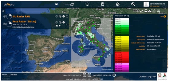
Figure 1.
Italian National Radar Network composite. Example of SRI (SRI adj in the figure) product together with geolocation of meteorological radar (green dots) (https://www.protezionecivile.gov.it/en/approfondimento/dewetra--versione-inglese-/, accessed on 12 February 2025). This is a screenshot of a platform not accessible to the public.
The radar dataset is based on the continuous period of 7 years from 1 January 2018 to 31 December 2024. A hindcast experiment was set up running the nowcasting model every 10 min, using the data at instant t and t − 10 min as input, following previous implementations set up of the model [28,29]. We thus have a large number of forecasts in a large domain that leads to a robust analysis.
It is important to highlight that rainfall data are used both as input to the nowcasting model and as observations for the verification process. Moreover, to avoid any misleading results, the implementation of the method was performed exclusively on deterministic advection of nowcasting.
All the single radars have several equations and techniques to filter out the observations and obtain the most reliable and correct rainfall maps. Moreover, the process of merging single maps in the Italian radar mosaic carries out more corrections. Despite all these factors, however, some random errors still affect the nowcasting input data (SRI) and need to be treated because nowcasting processes and related performances are largely affected by the presence of errors and artifacts in radar maps, especially the noise, that causes problems in the solution of small spatial scales [10].
A simple approach has been implemented to minimize the magnitude of errors, paying particular attention to ensuring that radar data errors do not influence the result, especially on small scales. It consists of a pass band filter that removes both cell spikes (e.g., random errors) and pixels below an intensity threshold (e.g., noise) under specific constraints. The threshold should be declared with a seasonal dependency, but as a first guess, it is set up at 1 mm/h, a value that affects only very low intensity events that are not of interest for applications in the field of flood forecasting and heavy rain warning. To avoid any loss of rainfall map structure information, the pre-processing filtering does not consist of a rigid cut-off of “negligible” values but is more accurate in terms of elimination strategies. Operationally, every identified cell is evaluated in terms of dimension (minimum size: 6 pixels) in order to filter out what is recognized as noise avoiding the reduction and the creation of holes or artifacts that could create losses of information especially at small scales.
As a final result of this pre-processing, only sparse and sporadic errors such as individual pixels with high values and precipitation structures with very low intensity that do not affect short-term forecast results were eliminated.
2.4. Identification of Calculation Domains
This section describes how the different approaches were studied and implemented with the goal of obtaining qualitative results in rapid computational time just to be suitable with the continuous updating of the radar images (5 min time resolution). The different approaches in identification of sub-domains and ability of interaction between cells are shown in Figure 2 and better described in the following bullet point paragraphs.
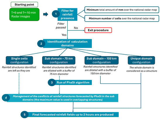
Figure 2.
Schematization with flow-chart approach of different PhaSt configurations. The first step of rainfall maps filtering is carried out. The four considered configuration schemes are then applied. In the single cell configuration, the problem of overlapping of rainfall structures forecasted by more than one sub-domain overlapping arises: in this case the maximum value for each pixel is considered.
- Benchmark (Unique domain—UD)
The very first trial is to consider a unique domain. This approach is derived from the analysis of a single radar where using the whole domain is the unique workflow as in the original version of the algorithm [10]. A pro of the routine is to also consider the large and very large scale that could work well with the synoptic scale events. Conversely, the unique domain brings up no discrimination of separate events, so the results are influenced by phase speeds calculated on a large scale and, in many cases, by long calculation times.
- 2.
- Sub-Domain 150 km (SD-150)
The first step in optimization was to adopt a sub-domain that separates rainfall cells that are very far and with no probability to converge. The method described in Section 2.2 defines the rainfall structures; subsequently, a spatial box of 150 × 150 km is centered recursively on each pixel of these structures and the maximum extensions along the x and y directions are considered to create a domain that is generally a rectangle. Once the rainfall structures are identified and confined in rectangular domains, it may be the case that two or more rectangles overlap, resulting in the possibility of a converging evolution. In SD-150 configuration this case is faced by merging the single rectangles into a single larger sub-domain.
The size of each rectangle was selected according to a median rain cell velocity observed over the Italian territory. The size of each rectangle was selected according to a median rain cell velocity observed over the Italian territory, that is 30km/h, corresponding to about 60 km in 2 h (horizon forecast of PhaSt).” Following this approach, the domain is split into sub-domains that have a minimum dimension of 150 km (which means more than twice in respect to 60 km) that are handled separately and finally merged in a unique map. From the computational-time point of view, on one hand we are dealing with a larger number of domains; on the other hand, the reduced size could help to obtain results in a very short time. The latter solution allows us to reduce the large scale’s problem described in the previous paragraph but does not completely solve the problem itself. The far single events are well described, but in case of mesoscale events composed by several structures disposed along a clear direction, these can still be treated as the unique domain losing some information on a very small scale. Once the forecast is carried out on each sub-domain, it is mapped onto the original unique domain.
- 3.
- Sub-Domain 75 km (SD-75)
The further adjustment has been to reduce even more the dimension of the rectangular cell that could contain a rainfall structure (the dimension of the box is decreased to 75 km). In this way the treatment of small cells could be more precise, and the capacity for adapting the dimensions does not affect very much the computational time since the number of sub-domains increases but their dimension decreases. The major achievement of this new approach is the possibility of merging different advected cells that lie in the same converging areas when single domain forecasts are mapped on the unique original domain. At first guess, the blending is assumed as the worst-case scenario, so the maximum values of nowcasted cells are kept in overlapping areas.
The combination of small sub-domains with the ability to unify the results can create a more dynamic and reliable nowcasting map.
- 4.
- Single Cells (SC)
The final approach discussed within this manuscript is the strictly defined shape of the sub-domain that contains rainfall structures. In fact, it is not even more limited within the box but it keeps the frame of the rain cells exactly with no extra domain. This trial is like an advective method but maintains the Fourier characteristic process. The main advantage of SC is to use the cells as they are extremizing the separation to follow the single trajectory and eventually merge in case of collision. From the point of view of computational time the effort is increased, but not sufficiently to dismiss the method.
The mapping of SC forecasts on the unique original domain was performed in the same way as for SD-75.
2.5. Implementation Strategy on Real Rainfall Maps
The identification of calculation domains as reported in the flow chart of Figure 2 could also be visually shown in Figure 3, where the decomposition of the SRI input map is demonstrated based on the different configurations described in the previous paragraphs. Each panel refers to the sub-domain definition obtained with the 4 methods: (A) UD; (B) SD-150; (C) SD-75; and (D) SC. Depending on the approach, a first identification is conducted and then a finalization in case of aggregation. The yellow rectangles represent the surrounding domain belonging to each cell present in the map, while the fuchsia ones symbolize the aggregation due to overlapping (if present in configuration). According to this description, the following should be recognized: (A) UD: 1 calculation domain independent from number of cells within (dimension: 1200 × 1400 pixels, calculation time: approximately 5 min); (B) SD-150: 7 cells identified with 6 overlapping lead to 2 calculation domains (dimension: from 150 × 150 to 600 × 600 pixels, calculation time: about 2 min); (C) SD-75: 7 cells identified with 4 overlapping leading to 4 calculation domains (dimension: from 150 × 150 to 300 × 600 pixels, calculation time: approximately 3 min); (D) SC: 7 cells identified corresponding to 7 calculation domains (dimension is cells-dependent from 30 × 30 to 150 × 150 pixels, calculation time: about 2 min).
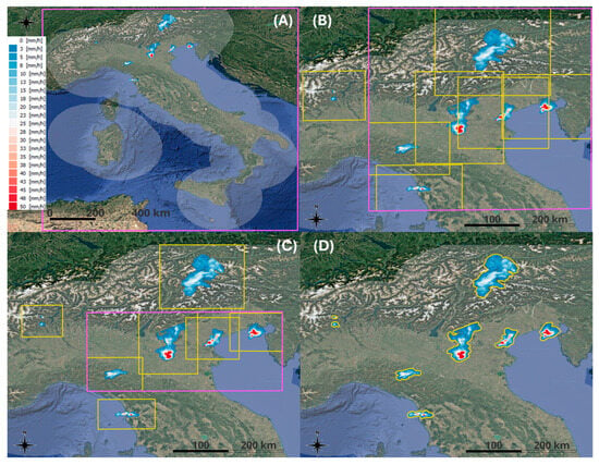
Figure 3.
Example of Surface Radar Intensity of the Italian radar composite on 2 August 2025 at 11:00 UTC and related sub-domains derived for the 4 considered configurations. Each sub-plot represents a setting as described above: (A) UD: 1 calculation domain independently from number of cells within; (B) SD-150: 7 cells identified (6 overlapping)—2 calculation domains; (C) SD-75: 7 cells identified (4 overlapping)—4 calculation domains; (D) SC: 7 cells identified—7 calculation domains.
2.6. Verification Methods
The performance analysis is based on the use of the contingency table and some standard verification metrics used for rainfall forecast. Referring to Table 1, the skill scores are reported in their applied formulation.

Table 1.
Contingency table applied to evaluate the skill scores.
Critical Success Index (CSI):
Heidke Skill Score (HSS):
Frequency Bias (FB):
The Hits, False Alarms, and Miss events have been calculated starting from the forecasted rainfall fields cumulated at an hourly scale and applying four thresholds (1-5-10-20 mm) to them. This choice is mainly due to the fact that the analysis is carried out with a hydrological perspective where rainfall accumulations are generally considered. Using the dichotomous matrix, the observed and forecasted rainfall maps have been compared, following a simple method inspired by the literature [30,31] in order to overcome the “double penalty effect”, according to which a forecasted rainfall field with correct size and structure of main rainfall cells but slightly wrong positioning can lead to very low verification scores. Hence, to overcome the “pixel to pixel” verification and avoid penalization due to small errors in positioning of the structures (resulting in more misses and false alarms), the scores have been calculated counting hits, false alarms and misses using buffers (Figure 4). This would also be consistent with the final operational purpose of the analyzed procedure: the criticality messages for civil protection purposes connected to heavy rainfall at the Italian scale are issued at municipality level, with an average dimension that can vary from less than 10 km2 to over 100 km2. For this reason, an accuracy at “pixel” level is unnecessary for this kind of application and a good compromise in the analysis is represented by the current use of the buffer verification.
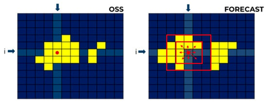
Figure 4.
Schematization of verification approach using a buffer around a pixel. Yellow pixels are those over a fixed threshold, red dot is an example of pixel where applying the contingency table, red rectangles represent the buffers where the procedure applies the contingency table to manage the double penalty issue.
In the present work two buffers are considered: 5 and 15 km.
3. Results
This section shows the results obtained from the 7-year analysis. First a visual example is reported to help in understanding the differences that come from each methodology, then the skill scores presented are applied to the three configurations analyzed (SD75, SD150, and SC) while the fourth configuration (UD) is reported as benchmark. Two hours of forecast are considered; boxplot representation was chosen in order to represent the variability of score values for each lead time.
3.1. Visual Example of Result
In this section a visual result of application of the configurations described in Section 2.4 is reported (see Figure 5), to appreciate the difference between the forecasted hourly accumulation (the very first hour) with respect to the observed Surface Rainfall Total (SRT). The reference input time is the SRI maps on 22nd May 2023 at 12:00 UTC, where several thunderstorms were sparsely distributed along the Apennines from Liguria to Calabria regions and on Sardinia. The comparison could be conducted through the different panels where (a) UD 1 h forecasted accumulation, (b) SD150 1 h forecasted accumulation, (c) SRT 1 h accumulation observation, (d) SD75 1 h forecasted accumulation, and (e) SC 1 h forecasted accumulation. Generally, in case of presence of several rainfall cells, the capacity of SD75 and even more of the SC is accentuated to preserve the single cell dynamic and obtain a good result, while the other methods tend to follow a median advection that cannot estimate the real dynamic, with the risk of concentrating an excess of rainfall volume where rainfall structures are larger in the observed field used as input, while failing to predict evolution of smaller storms.
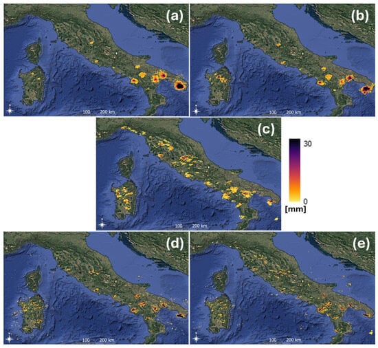
Figure 5.
Comparison between 1 h accumulation SRT observation (sub-panel (c)) and 1 h forecasted accumulation for (a) UD, (b) SD150, (d) SD75, and (e) SC.
3.2. Skill Scores Analysis
The graphs reported in Figure 6, Figure 7 and Figure 8 show the boxplot of the CSI, HSS, and FB for four different rainfall thresholds and considering a tolerance buffer of 5 km to compute skill scores. On the x axis the configurations are reported while the Y axis represents the score values.
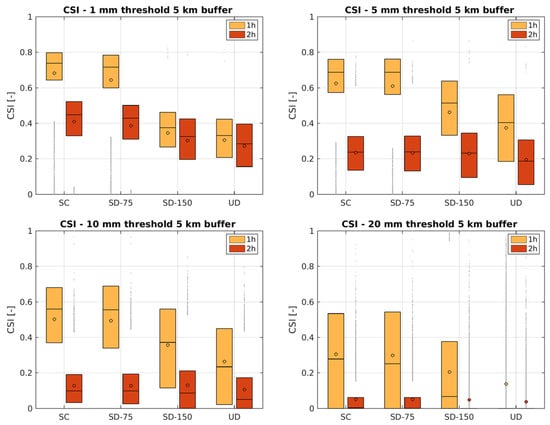
Figure 6.
CSI results for 5 km buffer. Rainfall accumulated in the first and second hour. Each boxplot represents the variability of CSI values for the 4 considered configurations: SC, SD-75, SD-150, UD.
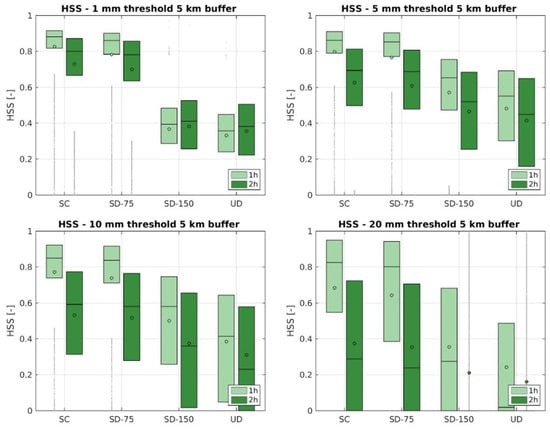
Figure 7.
HSS results for 5 km buffer. Rainfall accumulated in the first and second hour. Each boxplot represents the variability of HSS values for the 4 considered configurations: SC, SD-75, SD-150, UD.
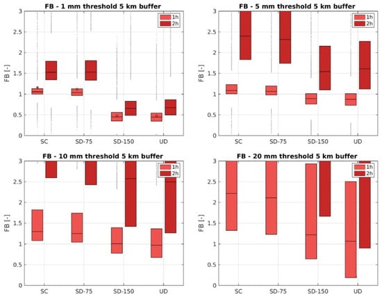
Figure 8.
FB results for 5 km buffer. Rainfall accumulated in the first and second hour. Each boxplot represents the variability of FB values for the 4 considered configurations: SC, SD-75, SD-150, UD.
Each configuration is drawn by two boxplots that consist of the first (light orange on the left in Figure 6) and second (dark orange on the right in Figure 6) hourly rainfall accumulation of nowcasting. Circles represent the average value. Graphs were created using all data relating to the 7-year period.
The CSI score is evidence that the single cell performs significantly better than the SD-150 one, while the SD-75 is more similar but, in any case, is averagely worse especially for 1 and 5 mm of the threshold. When considering the second hour of forecast, the differences are less noticeable, but this can be more related to the structural uncertainty of extrapolation nowcasting methods in capturing the correct forecast when lead time increases. When threshold is 20 mm the performance for the second hour of forecast is poor for all the configurations.
The UD shows the worst performance for all rainfall thresholds.
The HSS shows similar behavior of CSI. Even in this case performance is better for SC configuration, and the variability of results increases with the increase in threshold values. UD evidences the worst performance for all rainfall thresholds.
FB score introduces some other elements in the result interpretation. In this case, performance for SC is really similar to SD-75; in both cases FB is good for the first hour with values between 1 and 1.2 while evidence for SD-150 is a value lower than 1. Graphs show an increase in false alarms with respect to missing when the threshold increases. This behavior is particularly noticeable in the second hour of forecast, for the 20 mm threshold the FB values are larger than 3 and so are not visible on the graph.
FB for the 20 mm threshold is better for UD and SD-150 in respect to SD-75 and SC; box values are in fact closer to a value of 1 even if with very large variability. It must be highlighted that in this case, the data sample is smaller than for the lower thresholds.
Results when buffer is increased to 15 km show similar patterns and information for 5 km, though there is a general improvement of the performance due to a greater tolerance in considering the spatial location of observations with respect to the one of predictions. See Figure 9, Figure 10 and Figure 11.
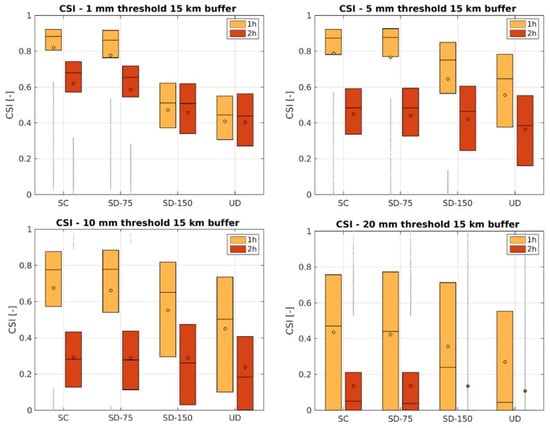
Figure 9.
CSI results for 15 km buffer. Rainfall accumulated in the first and second hour. Each boxplot represents the variability of CSI values for the 4 considered configurations: SC, SD-75, SD-150, UD.
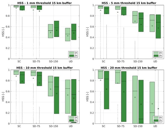
Figure 10.
HSS results for 15 km buffer. Rainfall accumulated in the first and second hour. Each boxplot represents the variability of HSS values for the 4 considered configurations: SC, SD-75, SD-150, UD.
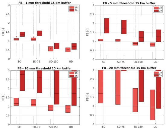
Figure 11.
FB results for 15 km buffer. Rainfall accumulated in the first and second hour. Each boxplot represents the variability of FB values for the 3 considered configurations: SC, SD-75, SD-150, UD.
4. Discussion
The present work explores some strategies of adaptation of a phase-diffusion model for rainfall nowcasting, with the aim of implementation at large spatial scales. Sub-domain dynamic and automatic setting is carried out with mathematical libraries for image elaboration. Configuration SD-150 tends to generate a few large calculation domains while SC creates domains around each single rainfall structure which produces a large number of domains especially when thunderstorms occur; SD-75 is an intermediate configuration between SD-150 and SC.
Results in terms of skill scores evidence that the usage of SC configuration leads to better performance; this is probably due to the fact that when phase velocities and amplitudes are estimated by Fast Fourier Transform, small domains allow us to better capture the variety of types of rainfall structures in terms of intensities, direction, and velocity of movements. Indeed, it is expected that over a large spatial domain such as the Italian territory, on an order of magnitude of hundreds or thousands of kilometers the in linear dimension, several rain events with very different characteristics may even be present at the same time. This physical condition seems to be best described by a subdivision into many small-scale computational domains, each propagating a particular type of rainfall structure in time and space. SD-150 and UD (the benchmark) show generally the worst performance even if FB for high rainfall thresholds (10, 20 mm) is comparable or even better with respect to the other configurations.
A comparison with other studies and methodologies can be made qualitatively by referring to the publications where they are presented. In [20], CSI versus lead time graphs are reported for rainfall rate, not for accumulation, and over a smaller area, but we can state that performances are comparable. Values are from 0.85 to 0.6, lead times 10–60 min, and threshold 1 mm/h; Figure 6 shows values around 0.7–0.75 on the hourly accumulation when SC and SD-75 are considered.
Ref. [22] shows performance of different methods at Italian scales; in this case, analysis is carried out using reflectivity thresholds (15, 25, 35 dBZ, which correspond approximately to 0.5, 1.5, 5 mm/h using the Marshall–Palmer Z-R). Even in this case we can state that SC and SD-75 perform similarly or even better.
Ref. [23] studies the effect of partition on macro-cluster of radar fields in terms of reflectivity; again, a direct comparison is not possible, but we can say that the performance of SC and SD-75 configurations are comparable.
The length of rainfall dataset of analysis leads authors to suppose a robustness of results and findings at least for the environment of experiment. Limitations of the work presented are definitely related to the particular type of algorithm used; the results therefore cannot be extended without further investigation into other types of nowcasting models. It is likely that other nowcasting methods benefit in a different way from computational domain decomposition strategies.
5. Conclusions
Rainfall nowcasting is still a challenging field of research due to the necessity of having correct quantitative prediction with low spatial errors especially in operational applications. This study demonstrates how a spectral nowcasting algorithm named PhaSt could operate on a large computational domain and some possible strategies of decomposition in smaller sub-domains that improve results in terms of standard skill scores. Specifically, a couple of the analyzed schemes that allow working on small sub-domains are promising in terms of improving forecasting. The main reason seems to be the improved description of the spectral characteristics of rainfall events observed in the sub-domains. Further studies could focus on applying the method in other environments or attempting to extend the approach to other nowcasting algorithms.
Author Contributions
Conceptualization, F.S., M.L.P. and F.P.; methodology, F.P. and M.L.P.; software, F.P. and M.L.P.; validation, F.S., M.L.P. and F.P.; formal analysis, M.L.P.; writing—original draft preparation, F.S. and M.L.P.; writing—review and editing, F.S., M.L.P. and F.P.; supervision, F.P. All authors have read and agreed to the published version of the manuscript.
Funding
This research was funded by the Italian Civil Protection Department, Presidency of the Council of Ministers, through the convention between the Italian Civil Protection Department and CIMA Research Foundation, for the development of knowledge, methodologies, technologies, and training, useful for the implementation of national systems of monitoring, prevention, and surveillance.
Data Availability Statement
The data presented in this study are available on request from the corresponding author due to large amount and internal ICT policy.
Acknowledgments
This work is supported by the Italian Civil Protection Department. We really thank Nicola Rebora for his support and precious suggestions.
Conflicts of Interest
The authors declare no conflicts of interest.
Abbreviations
The following abbreviations are used in this manuscript:
| UD | Unique Domain (benchmark) |
| SD150 | Sub-Domain 150 km |
| SD75 | Sub-Domain 75 km |
| SC | Single Cells |
| CSI | Critical Success Index |
| HSS | Heidke Skill Score |
| FB | Frequency Bias |
References
- Germann, U.; Zawadzki, I. Scale-Dependence of the Predictability of Precipitation from Continental Radar mages. Part I: Description of the Methodology. Mon. Weather. Rev. 2002, 130, 2859–2873. [Google Scholar] [CrossRef]
- Germann, U.; Zawadzki, I. Scale Dependence of the Predictability of Precipitation from Continental Radar Images.Part II: Probability Forecasts. J. Appl. Meteorol. 2004, 43, 74–89. [Google Scholar] [CrossRef]
- Li, L.; Schmid, W.; Joss, J. Nowcasting of Motion and Growth of Precipitation with Radar over a ComplexOrography. J. Appl. Meteorol. 1995, 34, 1286–1300. [Google Scholar] [CrossRef]
- Bowler, N.E.H.; Clive, E.P.; Seed, A. Development of a precipitation nowcasting algorithm based upon optical flow techniques. J. Hydrol. 2004, 288, 74–91. [Google Scholar] [CrossRef]
- Dixon, M.; Weiner, G. TITAN: Thunderstorm identification, tracking, analysis, and nowcasting—A radar-based methodology. J. Atmos. Ocean Technol. 1993, 10, 785–797. [Google Scholar] [CrossRef]
- Lang, P. Cell Tracking and Warning Indicators derived from Operational Radar Products. In Proceedings of the 30th International. Conference on Radar Meteorology, Munich, Germany, 19–24 July 2001; Available online: https://ams.confex.com/ams/pdfpapers/21678.pdf (accessed on 28 October 2025).
- Kyznarová, H.; Novák, P. CELLTRACK-Convective cell tracking algorithm and its use for deriving life cycle characteristics. Atmos. Res. 2009, 93, 317–327. [Google Scholar] [CrossRef]
- Bowler, N.E.; Pierce, C.E.; Seed, A.W. STEPS: A probabilistic precipitation forecasting scheme which merges an extrapolation nowcast with downscaled NWP. Q. J. R. Meteorol. Soc. 2006, 132, 2127–2155. [Google Scholar] [CrossRef]
- Seed, W. A Dynamic and Spatial Scaling Approach to Advection Forecasting. J. Appl. Meteorol. 2003, 42, 381–388. [Google Scholar] [CrossRef]
- Metta, S.; von Hardenberg, J.; Ferraris, L.; Rebora, N.; Provenzale, A. Precipitation nowcasting by a spectral-based nonlinear stochastic model. J. Hydrometeorol. 2009, 10, 1285–1297. [Google Scholar] [CrossRef]
- Zhang, Y.; Long, M.; Chen, K.; Xing, L.; Jin, R.; Jordan, M.I.; Wang, J. Skilful nowcasting of extreme precipitation with NowcastNet. Nature 2023, 619, 526–532. [Google Scholar] [CrossRef] [PubMed]
- Chen, S.; Zhang, S.; Geng, H.; Chen, Y.; Zhang, C.; Min, J. Strong Spatiotemporal Radar Echo Nowcasting Combining 3DCNN and Bi-Directional Convolutional LSTM. Atmosphere 2020, 11, 569. [Google Scholar] [CrossRef]
- Franch, G.; Tomasi, E.; Wanjari, R.; Poli, V.; Cardinali, C.; Alberoni, P.P.; Cristoforetti, M. GPTCast: A weather language model for precipitation nowcasting. Geosci. Model Dev. 2025, 18, 5351–5371. [Google Scholar] [CrossRef]
- Fabry, F. Nowcasting In Radar Meteorology: Principles and Practice; Cambridge University Press: Cambridge, UK, 2015; pp. 166–179, Chapter 10. [Google Scholar]
- Prudden, R.; Adams, S.V.; Kangin, D.; Robinson, N.H.; Ravuri, S.V.; Mohamed, S.; Arribas, A. A review of radar-based nowcasting of precipitation and applicable machine learning techniques. Environ. Sci. Comput. Sci. Eng. arXiv 2020. [Google Scholar] [CrossRef]
- Imhoff, R.O.; Brauer, C.C.; Overeem, A.; Weerts, A.H.; Uijlenhoet, R. Spatial and temporal evaluation of radar rainfall nowcasting techniques on 1,533 events. Water Resour. Res. 2020, 56, e2019WR026723. [Google Scholar] [CrossRef]
- Tan, Y.; Zhang, T.; Li, L.; Li, J. Radar-Based Precipitation Nowcasting Based on Improved U-Net Model. Remote Sens. 2024, 16, 1681. [Google Scholar] [CrossRef]
- Panziera, L.; Germann, U.; Gabella, M.; Mandapaka, P.V. NORA–Nowcasting of Orographic Rainfall by means of Analogues. Q. J. R. Meteorol. Soc. 2011, 137, 2106–2123. [Google Scholar] [CrossRef]
- Franch, G.; Nerini, D.; Pendesini, M.; Coviello, L.; Jurman, G.; Furlanello, C. Precipitation Nowcasting with Orographic Enhanced Stacked Generalization: Improving Deep Learning Predictions on Extreme Events. Atmosphere 2020, 11, 267. [Google Scholar] [CrossRef]
- Mazza, A.; Antonini, A.; Melani, S.; Ortolani, A. A Radar-Based Fast Code for Rainfall Nowcasting over the Tuscany Region. Remote Sens. 2025, 17, 2467. [Google Scholar] [CrossRef]
- Poli, V.; Bechini, R.; Cardinali, C.; Cremonini, R.; Alberoni, P.P. La Previsione a Brevissimo Termine Ottenuta Dal Blending di Estrapolazione Radar e Modellistica Numerica. IV Convegno Nazionale di Radar Meteorologia, Online. 2021. Available online: https://drive.google.com/file/d/1UGmiAL9UXRLdwYvlFoq4sr24RZ2sn39F/view (accessed on 28 October 2025).
- Gregori, V.; De Tomasi, F.; Ferrari, G.; Chini, A. A Comparison of Nowcasting Methods on the Italian Radar Mosaic. Master’s Thesis, Università degli Studi di Napoli Parthenope, Naples, Italy, 2020. Available online: http://master.meteorologiaeoceanografiafisica.unisalento.it/index.php/elaborati-degli-studenti (accessed on 28 October 2025).
- Montopoli, M.; Marzano, F.S.; Picciotti, E.; Vulpiani, G. Spatially-Adaptive Advection Radar Technique for Precipitation Mosaic Nowcasting. IEEE J. Sel. Top. Appl. Earth Obs. Remote Sens. 2012, 5, 874–884. [Google Scholar] [CrossRef]
- Vulpiani, G.; Guerriero, E.; Giordano, P.; Negri, M.; Pagliara, P. The Italian radar QPE: Description performance analysis and perspectives. In Proceedings of the 15th Plinius Conference on Mediterranean Risks, Giar-dini Naxos, Italy, 8–11 June 2016; Available online: https://meetingorganizer.copernicus.org/Plinius15/orals/22571 (accessed on 28 October 2025).
- Silvestro, F.; Rebora, N. Operational verification of a framework for the probabilistic nowcasting of river discharge in small and medium size basins. Nat. Hazards Earth Syst. Sci. 2012, 12, 763–776. [Google Scholar] [CrossRef]
- Poletti, M.L.; Silvestro, F.; Davolio, S.; Pignone, F.; Rebora, N. Using nowcasting technique and data assimilation in a meteorological model to improve very short range hydrological forecasts. Hydrol. Earth Syst. Sci. 2019, 23, 3823–3841. [Google Scholar] [CrossRef]
- Gilleland, E.; Ahijevych, D.; Brown, B.G.; Casati, B.; Ebert, E.E. Intercomparison of spatial forecast verification methods. Weather. Forecast. 2009, 24, 1416–1430. [Google Scholar] [CrossRef]
- Anthes, R.A. Regional models of the atmosphere in middle latitudes. Mon. Weather. Rev. 1983, 111, 1306–1335. [Google Scholar] [CrossRef]
- Vulpiani, G.; Montopoli, M.; Passeri, L.D.; Gioia, A.G.; Giordano, P.; Marzano, F.S. On the use of dual-polarized C-band radar for operational rainfall retrieval in mountainous areas. J. Appl. Meteorol. Climatol. 2012, 51, 405–425. [Google Scholar] [CrossRef]
- Silvestro, F.; Rebora, N.; Cummings, G.; Ferraris, L. Experiences of dealing with flash floods using an ensemble hydrological nowcasting chain: Implications of communication, accessibility and distribution of the results. J. Flood Risk Manag. 2015, 10, 446–462. [Google Scholar] [CrossRef]
- Poletti, M.L.; Lagasio, M.; Parodi, A.; Milelli, M.; Mazzarella, V.; Federico, S.; Campo, L.; Falzacappa, M.; Silvestro, F. Hydrological verification of two rainfall short-term forecasting methods with floods anticipation perspective. J. Hydrometeorol. 2024, 25, 541–561. [Google Scholar] [CrossRef]
Disclaimer/Publisher’s Note: The statements, opinions and data contained in all publications are solely those of the individual author(s) and contributor(s) and not of MDPI and/or the editor(s). MDPI and/or the editor(s) disclaim responsibility for any injury to people or property resulting from any ideas, methods, instructions or products referred to in the content. |
© 2025 by the authors. Licensee MDPI, Basel, Switzerland. This article is an open access article distributed under the terms and conditions of the Creative Commons Attribution (CC BY) license (https://creativecommons.org/licenses/by/4.0/).