Abstract
Vertical line source irrigation is a localized water-saving technique suitable for deep-rooted crops, but the geometric structure of the wetted bulb lacks a systematic analytical modeling method. This study established a simplified three-dimensional (3D) analytical model to predict the wetted volume under vertical line source irrigation conditions. First, the model determined boundary points based on an empirical wetting-front equation and fitted the wetting profile with ellipse–parabola functions to derive analytical expressions for area and volume. Then, using aeolian sandy soil as the research object, the model predicted that during 0–250 min of irrigation, the wetted pattern area increased from 80.0 cm2 to 5050.6 cm2, and the wetted volume increased from 251.3 cm3 to 208,014.4 cm3. At 250 min, the lower, middle, and upper volume components accounted for 67.3%, 24.2%, and 8.4%, respectively. Finally, the model was validated using loam soil, and the results showed good agreement between the calculated and measured values. The model requires only simple input and enables fast computation. It effectively characterizes the three-dimensional spatiotemporal variation of the wetted bulb and provides a theoretical reference for the design of pipe spacing and irrigation quota.
1. Introduction
Water scarcity had become a major limiting factor for sustainable agricultural development in arid and semi-arid regions [1]. Improving water use efficiency had therefore become an important goal in modern irrigation research. Among various water-saving irrigation methods, micro-irrigation technologies such as drip irrigation were widely used due to their low energy consumption and high water use efficiency [2]. However, for deep-rooted or perennial crops, traditional drip irrigation systems often failed to supply water effectively to the deep root zone, which limited crop yield and water productivity.
To address this problem, an improved irrigation method called Vertical Line Source Irrigation was proposed. Vertical line source irrigation delivered water directly to the lower root zone through vertically buried porous pipes, which effectively reduced surface evaporation loss and improved the distribution of soil moisture in deeper layers. To achieve refined design of micro-irrigation systems, scholars at home and abroad have conducted extensive studies on soil wetting patterns under different irrigation methods.
At present, various models have been proposed to describe wetting patterns. These models can be mainly divided into three categories: analytical models, numerical models, and empirical models.
Among them, analytical models usually solve the basic equations of soil water movement, to obtain analytical or semi-analytical solutions of the wetting front position under given initial and boundary conditions. These models often use soil hydraulic parameters and emitter flow rate as key variables, to predict the depth and width of the wetted bulb in soil [3,4]. Philip [5] used quasi-linear analysis based on three-dimensional unsaturated steady flow, and derived analytical solutions for the water movement time from surface and buried point sources. He pointed out that near the source, the flow is mainly dominated by capillary force and shows symmetrical characteristics. Moncef and Khemaies [6] assumed the wetted bulb to be a semi-ellipsoid. Based on the Green-Ampt theory, they derived analytical formulas for the wetting front position and the wetted bulb volume in soil. These formulas can be used to predict the depth and width of the wetting pattern under specific soil hydraulic parameters. Cook et al. [7] derived the radius–time relationship of the wetted zone for both surface and subsurface point sources. They simplified and extended the theoretical calculation by using an exponential function form of soil water diffusivity. Chu [8] proposed an “infiltration capacity curve” to describe the relationship between the wetted bulb volume and time under a surface point source (emitter). This provided a calculable theoretical basis for the design of drip irrigation systems. Thorburn et al. [9] used Philip’s analytical infiltration model to systematically analyze the wetting patterns of emitters under different soil conditions. This provided a theoretical basis for the design of drip irrigation systems. Kilic [10] proposed a three-dimensional analytical method based on laboratory experiments. The method used four parabolic functions to quantitatively describe the spatial and temporal variations of the drip irrigation wetting pattern. However, this method was only suitable for geometric description after infiltration occurred. It could not rapidly predict the wetted bulb volume at different times based on soil hydraulic parameters.
Numerical models simulate variably saturated soil water movement by solving the Richards equation or its simplified forms. They can account for complex processes such as irregular boundaries, soil heterogeneity, and root water uptake [11,12]. HYDRUS-2D/3D is one of the most commonly used numerical simulation tools at present. It has been widely applied to the study of wetting patterns under various irrigation methods such as drip and subsurface irrigation. Studies have shown that numerical models have high prediction accuracy under different soil conditions [13]. For example, Elmaloglou and Diamantopoulos [14], considering the hysteresis effect of soil moisture, successfully simulated the water redistribution process of the surface drip irrigation wetted bulb based on a cylindrical symmetric flow model; The propagation of the wetting front under subsurface drip irrigation conditions was studied by Qiao et al. [15] through experiments and numerical simulations. A dimension analysis-based model for estimating the wetting front was proposed. This model effectively addresses the problem of predicting soil wetting fronts and can accurately estimate the propagation pattern of the wetting front in sandy soils.Lazarovitch et al. [16] built a training dataset using HYDRUS-2D and trained an artificial neural network to directly predict the soil water distribution around the emitter. They compared three types of outputs, and the results showed that the model using spatial moments was the most stable. It could be used for rapid estimation and design optimization of the wetted pattern under drip irrigation.
Empirical models are mainly developed through regression analysis and dimensional analysis of experimental data or numerical simulation results. They usually take soil hydraulic properties and emitter flow rate as independent variables, to predict the depth and width of the wetting pattern. For example, Elmaloglou and Malamos [17], considering root water uptake and evaporation, used a cylindrical flow model to predict the width and depth of the wetted bulb. Bhatnagar and Chauhan [18] proposed an unsteady and nonlinear numerical model in an oblate spheroidal coordinate system, to simulate wetting front advancement and the geometric characteristics of the wetted bulb under surface drip irrigation. To solve the problem of the difficulty in quickly estimating the wetted dimensions in drip irrigation design, Al-Ogaidi et al. [19] used multi-source field data and proposed an improved empirical model based on nonlinear regression. The model explicitly predicted the wetted radius and depth, providing support for emitter spacing and irrigation management decisions. Naglič et al. [20] used HYDRUS-2D/3D, which applies the finite element solution of the Richards equation, together with dynamic surface drip irrigation boundary conditions, to conduct systematic numerical simulations. They described how the wetted radius and depth responded to irrigation volume and operating conditions and verified the results through soil tank experiments. Malek and Peters [21] performed regression analysis using field data from Karaj, Iran, and proposed a new empirical formula to directly predict the soil wetted dimensions around the emitter. This approach significantly reduced the computational cost and parameter requirements during the design stage. Amin and Ekhmaj [22] collected a large number of field data from both domestic and international studies and developed an empirical model using nonlinear regression analysis. The model could directly predict the size of the wetted pattern area in drip irrigation based on irrigation volume, emitter flow rate, soil hydraulic conductivity, and changes in soil water content. Schwartzman and Zur [23] proposed a semi-empirical method. Based on the simulation results of two-dimensional and three-dimensional infiltration models together with experimental data, they established quantitative relationships between the geometry of the wetted bulb and factors such as soil properties, emitter flow rate, and irrigation volume. This provided a basis for rapid on-site estimation. Fan et al. [24] conducted numerical simulations of wetting front movement and soil moisture distribution under vertical line source irrigation using HYDRUS-2D (Version 2.05), and proposed an empirical model, but did not develop a 3D model of the wetted bulb volume.
These studies provided an important basis for understanding the law of soil water movement. However, most existing models were based on point-source or surface-source infiltration assumptions and could not accurately describe the asymmetric expansion of the wetted bulb along the depth under vertical line source irrigation conditions. In addition, although three-dimensional numerical models could simulate water movement with good accuracy, they required heavy computation and many parameters. In fact, although most empirical models are widely used, they can only estimate the wetted radius and depth on a vertical cross-section [10] and lack analytical descriptions and rapid prediction models for the 3D wetted bulb volume. Therefore, it was necessary to develop an analytical model suitable for vertical line source irrigation to enable rapid prediction of the wetted bulb volume under such conditions.
Based on the above problems, this study focused on three-dimensional modeling of the wetted bulb under vertical line source irrigation conditions and proposed a simplified three-dimensional analytical model to predict the wetted bulb volume and its spatiotemporal variation. First, the boundary point coordinates were determined from the position of the wetting front, and then the boundary was fitted using ellipse–parabola functions to build analytical models of the area and volume. Finally, aeolian sandy soil was used as a case for analysis, and measured data from silty loam soil were used to verify the model. The model had a simple structure and required few parameters. It could quickly calculate the three-dimensional wetted bulb volume, overcoming the limitations of existing models that lacked analytical formulation under vertical line source irrigation conditions, and showed good innovation and practical value.
2. Materials and Methods
To provide a clearer understanding of the logical framework and key steps of the model construction, Figure 1 illustrated the overall research process for developing the analytical model of the three-dimensional wetted bulb under vertical line-source irrigation. This could serve as a reference for design optimization and model application in similar irrigation systems.
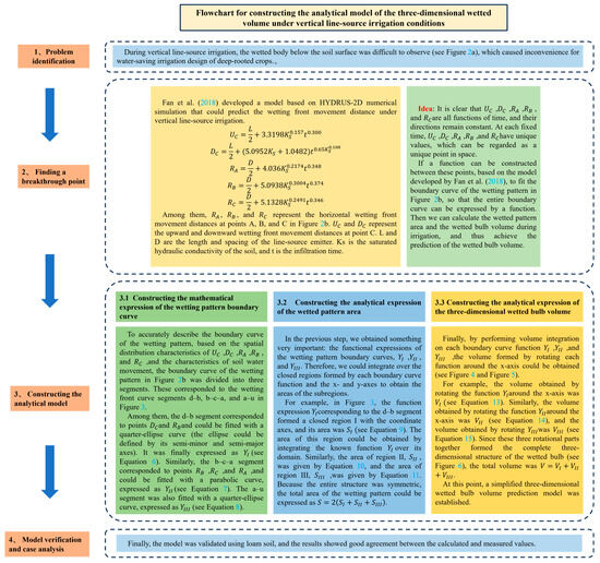
Figure 1.
Flowchart of the construction process of the analytical model for the three-dimensional wetted bulb under vertical line-source irrigation. Figure citation ‘Fan et al. (2018)’ refers to reference [25].
This study focused on the geometric modeling and analytical expression of the wetted bulb structure under vertical line source irrigation conditions, and divided the entire modeling process into four stages, as follows:
In the first stage, based on the wetting front movement prediction model (empirical model) developed by Fan et al. [25], wetting front movement formulas in five directions at three key points (Equations (1)–(5)) were introduced, to identify the variation patterns of water movement in each direction, providing a mathematical basis for constructing the analytical expressions of the wetting pattern boundary in the following steps.
In the second stage, based on the coordinates of the wetting pattern boundary points () determined by the empirical model (see Figure 2 and Figure 3), analytical expressions suitable for the boundary curves of the wetting pattern were constructed. According to the diffusion characteristics of soil moisture in different directions, the wetting profile was divided into three subregions, and ellipse and parabola functions were used for curve fitting in each subregion. This completed the functional modeling of the two-dimensional structure of the wetting pattern.
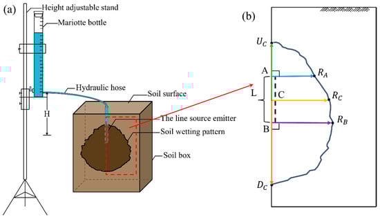
Figure 2.
(a) Schematic diagram of experimental equipment (H represents inlet pressure head); (b) Schematic diagram of key points and wetting front movement directions of the line source emitter (, , and represent the horizontal wetting front movement distances at points A, B, and C, respectively; and represent the upward and downward wetting front movement distances at point C, respectively).
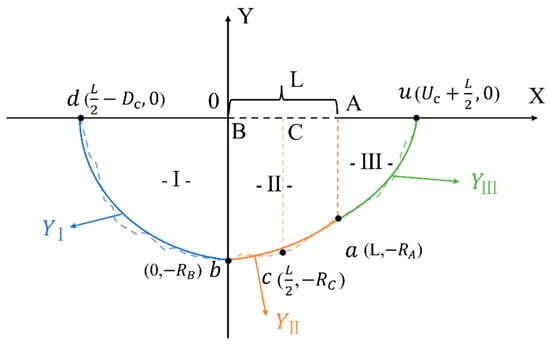
Figure 3.
Schematic diagram of the three-region division and boundary functions of the wetting pattern under vertical line source irrigation.
In the third stage, based on the analytical expressions, an area model of the wetting pattern was established. A three-dimensional volume model was constructed by rotating the analytical expressions around the x-axis. This enabled accurate description of the geometric structure of the wetted bulb.
In the fourth stage, aeolian sandy soil was selected. The model was run to output the changes in the area of the wetting pattern and the 3D wetted bulb volume under different irrigation durations. A multidimensional analysis was carried out to verify the applicability of the model.
The primary objective of the first stage was to present and analyze the wetting front movement prediction model for vertical line source irrigation developed by Fan et al. [25] using HYDRUS-2D numerical simulations. This empirical model used the structural characteristics of the line source emitter (the dashed part in Figure 2b), including length () and diameter (), as well as soil physical parameters (saturated hydraulic conductivity ) and infiltration time () as independent variables, to predict the wetting front movement distances in different directions from the top (A), bottom (B), and center (C) of the line source emitter.
Figure 2 was drawn to clearly show the physical context of the study and the corresponding relationships of key infiltration parameters. Figure 2a shows the vertical line source irrigation experimental setup used by Fan et al. [25], The experiment device consists of five parts: a height adjustable stand, a mariotte bottle, a hydraulic hose, a line source emitter, and a soil box.
The empirical model includes five prediction formulas (Equations (1)–(5)), which are used to estimate the wetting front movement distances in the vertical direction at point C (, ) and in the horizontal direction at points A, B, and C (, , ) (see Figure 2b). These formulas adopt a power function form, representing the nonlinear variation of wetting front movement distance over time.
In the equations, and represent the length and width of the line source emitter, respectively, cm; is the saturated hydraulic conductivity of the soil, cm/min; is the infiltration time, min.
To further analyze the spatial diffusion characteristics of water in soil under vertical line source irrigation conditions, the second stage was based on the empirical model from the previous stage and constructed mathematical expressions for the boundary curves of the wetting pattern, and carried out geometric modeling analysis of the wetting pattern.
To illustrate how the multidirectional infiltration process was transformed into an analyzable boundary representation, Figure 3 showed the partition logic and mathematical modeling approach of the wetting pattern.
First, to construct the mathematical expressions of the wetting pattern boundary curves, we referred to the method proposed by Kilic [10]. The soil wetting pattern in Figure 2b was rotated 90 degrees clockwise, and a Cartesian coordinate system was established with point B as the origin, forming the geometric structure shown in Figure 3.
To accurately describe the boundary curves of the wetting pattern under vertical line source irrigation conditions, the curve was divided into three structural segments, corresponding to the wetting front curve segments shown in Figure 3, namely the segment, the segment, and the segment.
Region I (the area enclosed by segment and the coordinate axis in Figure 3): represents the region below the line source emitter where water diffuses under the influence of gravitational potential. It can be fitted with a quarter-ellipse curve, corresponding to the boundary function ;
Region II (the area enclosed by segment and the coordinate axis in Figure 3): represents the wetted area formed by lateral diffusion of water in the horizontal direction. A parabolic curve can be fitted based on the coordinates of the three boundary points and corresponding to the boundary function .
Region III (the area enclosed by segment and the coordinate axis in Figure 3): represents the region above the line source emitter where water infiltrates upward. It is also fitted with a quarter-ellipse curve, corresponding to the boundary function .
The coordinate values of the key points () on each regional boundary were all determined using the previously mentioned prediction model (Equations (1)–(5)).
These structural divisions were determined based on the variation characteristics of water diffusion in soil under vertical line source irrigation. At the early stage of irrigation, soil water movement was mainly dominated by matric potential. The wetting front moved fastest in the horizontal direction. As time passed, gravitational potential began to play a dominant role. The downward vertical wetting front eventually moved farther than those in the horizontal and upward vertical directions [26] (pp. 44–45).
Based on this physical characteristic, selecting different types of curves for different regions better reflects the characteristics of water movement. After comparison, the combination of ellipse and parabola functions was found to be optimal in terms of fitting accuracy and structural interpretability. Therefore, the following expressions were adopted:
Function :
where and are the semi-axis lengths in the and directions, respectively.
Function :
Function :
Among them, variables such as ,, , , and were provided by the prediction formulas in the first stage. Thus, we obtained the approximate functional expressions , and describing the boundary curves of the wetting pattern in each region.
Through the above regional modeling, we laid the foundation for the analytical expression of the area of the wetting pattern and the wetted soil volume in the next stage and provided a basis for the subsequent 3D modeling.
To achieve geometric quantification of the wetted bulb under Vertical line source irrigation conditions, the third stage was based on the functional expressions established in the second stage and incorporated the structure of the soil wetting pattern shown in Figure 3, to construct an area model of the wetting pattern and a 3D volume model formed by its rotation around the x-axis.
2.1. Analytical Description of the Area of the Wetting Pattern
To clearly explain the geometric analysis process of the wetted pattern area and its positional relationship within the structure, Figure 4 showed the mathematical method used to derive the wetted pattern area expression from the piecewise boundary functions in the model development.
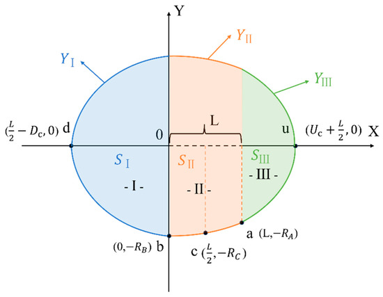
Figure 4.
Schematic diagram of the symmetrical mapping and area regions of the wetting pattern under Vertical line source irrigation.
As shown in Figure 4, the wetting profile below the x-axis was mirrored across the x-axis, resulting in a fully symmetrical geometric structure. Based on the regional divisions defined in the second stage (see Figure 3), the following sections calculate the area enclosed by each region below the x-axis in sequence.
Area of Region I ():
The area of this region can be directly expressed using the formula for a quarter ellipse, yielding the following analytical expression:
Area of Region II ():
The area of this region can be expressed as:
By expanding the integrand and integrating term by term, the analytical expression is obtained as:
Area of Region III ():
The area of this region can be directly expressed using the quarter-ellipse formula, yielding the analytical expression:
Since the entire structure is symmetrical, the total area of the wetting pattern can be expressed as:
2.2. Analytical Description of the 3D Volume of the Wetted Bulb
To provide a clearer understanding of how the volume expressions of each part were derived and to show the overall three-dimensional shape of the soil wetted bulb, Figure 5 and Figure 6 were drawn.
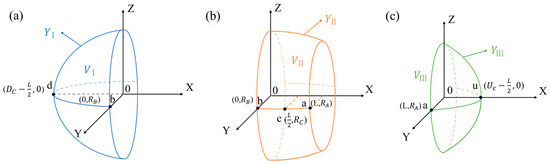
Figure 5.
(a) The three-dimensional volume structure () formed by rotating the function curve around the x-axis; (b) The three-dimensional volume structure () formed by rotating the function curve around the x-axis; (c) The three-dimensional volume structure () formed by rotating the function curve around the x-axis.
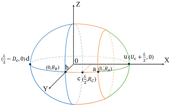
Figure 6.
Schematic diagram of the three-dimensional spatial division and volume composition of the wetted bulb under Vertical line source irrigation.
According to the structure shown in Figure 5, the three-dimensional wetted bulb was formed by rotating the function curves , and around the x-axis. To further analyze the volume composition, the volume expressions formed by the rotation of each curve are derived one by one below.
As shown in Figure 5a, the volume generated by rotating the function around the x-axis was denoted as , and its analytical expression is as follows:
As shown in Figure 5b, the volume generated by rotating the function around the x-axis is denoted as , and its analytical expression is as follows:
By expanding the integrand and integrating term by term, the analytical expression was obtained as:
As shown in Figure 5c, the volume generated by rotating the function around the x-axis was denoted as , and its analytical expression is as follows:
The three rotational parts together form the complete three-dimensional structure of the wetted bulb (see Figure 6), and the total volume is:
In the next stage of the study, the designed model was run using experimental data, and the results were analyzed.
2.3. Wetting Front Movement Characteristics in Different Directions Under Aeolian Sandy Soil Conditions
To evaluate the applicability and dynamic performance of the constructed area model of the wetting pattern and the three-dimensional wetted bulb volume model, this study used aeolian sandy soil ( = 0.345 cm/min) from the experiment conducted by Fan et al. [25] for modeling and calculation. A systematic analysis was then carried out based on the simulation results.
To illustrate the performance of the prediction model (Equations (1)–(5)) in simulating the time-dependent wetting front movement under aeolian sandy soil conditions, Figure 7 shows the variation curves of the wetting front distance over 0–250 min in five directions (, , , and ).
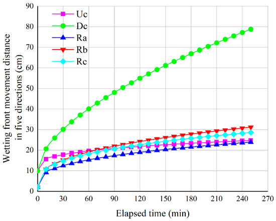
Figure 7.
Comparison of wetting front movement trends in five directions under aeolian sandy soil conditions.
As shown in Figure 7, the wetting front movement distance in the direction was consistently much greater than in the other directions. This phenomenon is not only caused by the dominant role of gravitational potential in the vertical direction but is also closely related to the hydraulic properties of the aeolian sandy soil itself.
2.4. Variation Characteristics of Wetted Area and Volume During Irrigation
To more intuitively illustrate the variation characteristics of area () and volume () during the irrigation process, the model output results in Table 1 were used as the basis, and Figure 8, Figure 9, Figure 10, Figure 11 and Figure 12 were compiled and plotted accordingly, followed by a multi-angle analysis of their variation characteristics.

Table 1.
Analytical model results of wetting pattern area and wetted bulb volume under different irrigation durations.
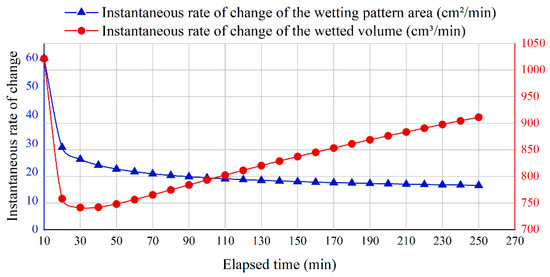
Figure 8.
Instantaneous spatio-temporal rate of change of the area of the wetting pattern () and the volume of the wetted bulb ().
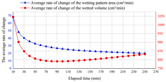
Figure 9.
The average rate of change of the wetting pattern area () and the wetted bulb volume () over the spatio-temporal domain.
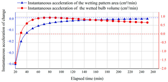
Figure 10.
The instantaneous acceleration of the wetting pattern area () and the wetted bulb volume ().
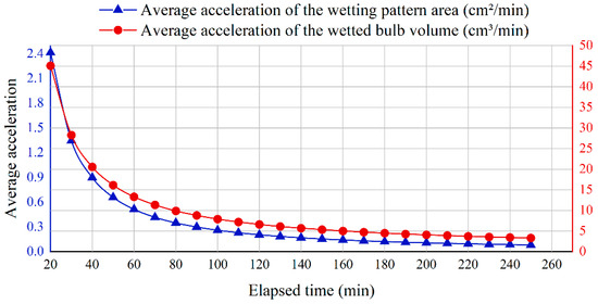
Figure 11.
Average acceleration of the wetting pattern area () and the wetted bulb volume () in vertical line source irrigation system.
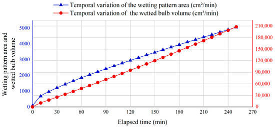
Figure 12.
Temporal variation of the wetting pattern area () and the wetted bulb volume ().
Figure 8 shows the instantaneous change rates of the wetting pattern area () and wetted bulb volume () at different time points, which are used to characterize the real-time variation in growth rate. Figure 9 presents the average change rates of both parameters, which reflect the growth rate per unit time.
As shown in Figure 8 and Figure 9, the change rate of the area continuously decreased throughout the irrigation process, indicating that water diffusion gradually slowed down, and the area of the wetting pattern tended to stabilize. In contrast, the volume change rate first dropped to its lowest point (around 30 min) and then gradually increased. This suggests that water mainly migrated in the vertical downward direction after that, resulting in a continuous increase in the thickness of the wetted bulb, which in turn drove the continued growth of the total volume.
Figure 10 and Figure 11 showed the changes in instantaneous and average acceleration of the wetted pattern area and soil wetted bulb volume over time. As shown in Figure 10, the instantaneous acceleration of the wetted pattern area remained negative and gradually approached zero. In contrast, the instantaneous acceleration of the soil wetted bulb volume changed from negative to positive at about 30 min, reached its peak at around 70 min, and then slowly decreased.
Figure 12 further showed the time variation of the wetted pattern area and wetted bulb volume during the entire irrigation period. It could be seen that the volume increased steadily in a nearly linear way, while the area also showed a clear overall increase but with a slightly slower growth rate in the middle and later stages. The growth trend of area was slightly weaker than that of volume. This was consistent with the natural water movement characteristics in sandy soil.
3. Results and Discussion
3.1. Analytical Model Results of Wetting Pattern Area and Wetted Bulb Volume Under Different Irrigation Durations
To comprehensively demonstrate the spatial applicability of the area and volume models of the wetting pattern developed in this study, Table 1 presents the calculated results of the areas (, , ) enclosed by the boundary curves (, , ), as well as the volumes (, , ) generated by their rotation around the x-axis.
In Table 1, the area of the wetting pattern, , is composed of the sum of three sub-areas (), which reflects the area variation of the wetting pattern. The wetted bulb volume, , is the sum of the sub-volumes (), representing the volume variation of the entire wetted bulb in 3D space.
Table 1 shows the time-dependent variation trends of area and volume calculated by the analytical model, which are consistent with the natural water diffusion process in aeolian sandy soil. At 250 min, the lower, middle, and upper volume components accounted for 67.3%, 24.2%, and 8.4%, respectively.
3.2. Supplementary Validation
To verify the reliability of the prediction formulas (Equations (1)–(5)), Fan et al. [25] used sandy loam (bulk density = 1.45 g/cm3, field capacity = 0.332 cm3/cm3, saturated hydraulic conductivity = 0.039 cm/min) and aeolian sand ( = 1.56 g/cm3, = 0.051 cm3/cm3, = 0.345 cm/min) from Minqin County, Wuwei City, Gansu Province, China, for vertical line source irrigation tests. Two treatments were applied to each soil, and the tests were repeated three times.
The results showed that the mean absolute error (MAE) and root mean square error (RMSE) were both close to zero. The percent bias (PBIAS) ranged between −4% and 9%, and the Nash–Sutcliffe efficiency coefficient (NSE) was not lower than 0.929. These results confirmed that the empirical model had high prediction accuracy.
To verify the universality and reliability of the area and volume models of the wetting pattern developed in this study, this study used the vertical line-source infiltration experiment conducted by Fan [26] under loam soil conditions (saturated hydraulic conductivity = 0.0143 cm⋅min−1. Five observed values of the wetting front movement distance at different times (pp. 14–21) were extracted from the experiment. These observed data were compared with the model calculation results; the evaluation indices included MAE, RMSE, NSE, and PBIAS (see Table 2).
Table 2.
Comparison between calculated and observed wetting-front movement distances under loam soil conditions.
It should be noted that, due to limited data availability, the publicly available literature still lacked measured data on the wetted bulb volume under vertical line-source irrigation conditions. Because the movement of the wetting front was closely related to the expansion of the wetted bulb volume, and the two showed consistent temporal trends, this study used the change in wetting-front movement distance as a reasonable proxy for the change in wetting-body volume to approximately reflect the generality of the model.
As shown in Table 2, the calculated wetting-front characteristic values were generally consistent with the observed values. A statistical analysis of the calculated and observed values showed that MAE was 0.506 cm, RMSE was 0.522 cm, PBIAS was −0.284, and NSE was 0.960. These results indicated a good agreement between the calculated and observed values.
3.3. Analysis of the Dynamic Variation of the Wetted Pattern Area and Soil Wetted Bulb Volume, and the Infiltration Mechanism
As shown in Figure 7, the migration distance of the wetting front in the Dc direction was always significantly greater than that in other directions. This trend was consistent with the numerical results reported by Fan et al. [24] for the vertical line source irrigation condition, where the wetting pattern showed an approximately ellipsoidal distribution with dominant vertical extension under gravity. Unlike traditional point-source models [5,8], Vertical line source irrigation represented a line-source water supply. Its geometric boundary and supply mode were fundamentally different, so the wetted bulb showed distinct spatiotemporal evolution characteristics compared with point-source conditions. Kilic [10] proposed a three-dimensional analytical model based on point-source drip irrigation to predict the wetted bulb volume. He found that under point-source drip irrigation, the wetted bulb was more evenly distributed horizontally. This differed from the results in Figure 7, indicating that continuous line-source water supply could more effectively promote the formation of deeper wetted zones, showing a different infiltration behavior from that of point-source drip irrigation.
Figure 7 clearly illustrated the expansion pattern of the wetting front over time under vertical line-source condition. The result revealed the characteristics of gravity-dominated vertical infiltration and provided a new perspective for understanding water redistribution under line-source irrigation.
As shown in Figure 8 and Figure 9, the rate of change of the wetted pattern area () continuously decreased during the entire irrigation process. This indicated that as time passed, the soil pores gradually became filled with water, the potential for horizontal diffusion weakened, and the rate of water expansion slowed down [27], causing the wetted pattern area to approach stability. The rate of change of the wetted bulb volume () reached its lowest point at around 30 min and then gradually increased. This suggested that after the initial stage dominated by capillary forces ended, gravity infiltration became dominant. Water mainly moved downward along the vertical direction—a phenomenon widely reported in the literature—causing the thickness of the wetted bulb to keep increasing. Even though horizontal expansion slowed down, the total volume continued to grow. This phenomenon was consistent with the characteristics of sandy soils, which have high permeability and low capillary retention, indicating that the model could reasonably represent the actual process of water movement.
Figure 10 and Figure 11 further revealed, through the change in acceleration, the variation of the wetted pattern area and soil wetted bulb volume during the irrigation process. The acceleration of the wetted pattern area remained negative and gradually approached zero, indicating that the expansion process gradually entered a stable stage. The acceleration of the soil wetted bulb volume changed from negative to positive at about 30 min, reached its peak at around 70 min, and then slowly decreased. This characteristic once again reflected the interaction between capillary action and gravity infiltration during the infiltration process. In the early stage, soil suction dominated, and the growth rate gradually decreased; in the middle and later stages, as the effect of gravity increased, the volume growth accelerated again.
Figure 12 shows the temporal evolution of the wetted pattern area and soil wetted bulb volume during the entire irrigation period. It can be seen that the soil wetted bulb volume increased almost linearly with time, while the wetted pattern area also increased significantly overall but showed a slightly slower growth rate in the middle and later stages. Overall, the growth trend of volume was stronger than that of area expansion, which was consistent with the actual situation under natural conditions.
Figure 8, Figure 9, Figure 10, Figure 11 and Figure 12, based on an analytical geometric model, quantitatively introduced the instantaneous rate of change and acceleration of the wetted pattern area and soil wetted bulb volume. These analyses revealed the dynamic three-dimensional expansion pattern of the wetted bulb under vertical line-source irrigation. This deepened the understanding of the coupling mechanism between capillary action and gravity infiltration and provided a theoretical reference for pipe spacing layout and water amount optimization in irrigation system design.
3.4. Discussion on Model Applicability and Limitations
The wetted bulb volume prediction model proposed in this study for vertical line source irrigation is applicable to different soil textures, emitter structure parameters, and various irrigation durations. Although the shape of the wetted bulb varies under different conditions, the core variables and analytical parameters of the model were developed based on the fundamental movement patterns of the wetting front in all directions. Therefore, when applied under different conditions, it only requires the input of key wetting front parameters (such as , , , and ) to quickly determine the three-dimensional wetted bulb volume at any given time using the proposed model.
In addition, the soil wetted bulb volume prediction model developed in this study for vertical line-source irrigation accurately described the changes of the wetted bulb in space and time during irrigation. It also provided a basis for the design and operation optimization of vertical line-source irrigation systems. Specifically, key parameters from the model, such as the maximum horizontal expansion radius () and the vertical advancement depth (), could be used to assess how adjacent wetted bodies were distributed under different pipe spacing conditions. This helped build a quantitative relationship between the geometric characteristics of the wetted bulb and pipe spacing, providing a theoretical basis for optimizing irrigation system layout. At the same time, the model’s prediction of the rate of wetted bulb volume change could be used to determine the best irrigation duration and frequency needed to reach an effective wetting depth. This achieved a smooth connection between water movement simulation and irrigation control optimization.
It is worth noting that although Fan et al. [25] verified the reliability of the empirical model (Equations (1)–(5)) through soil box experiments, there were still some deviations. One possible reason is that the wetting front movement distance under vertical line source irrigation is most strongly affected by soil texture, while initial soil moisture content, as well as the emitter’s diameter, length, and burial depth, also have some influence. To simplify the calculations, only soil texture was considered, and a single-variable model was established, which, to some extent, affected the accuracy of the results. In addition, using only the saturated hydraulic conductivity () to represent the wetting front movement behavior in different soil textures is also one of the sources of error.
4. Conclusions
This study focused on the soil water movement under vertical line-source irrigation and proposed a three-dimensional wetted bulb prediction model based on analytical geometry principles. The model described the shape of the wetting front by introducing a piecewise composite curve (a combination of an ellipse and a parabola). With only a few key parameters such as , , , and , it allowed fast calculation of the wetted bulb volume and wetted pattern area. Compared with traditional numerical models based on the Richards equation (such as HYDRUS-2D/3D), this model maintained reasonable accuracy while greatly reducing parameter requirements and computational complexity. It showed good repeatability and practical applicability for engineering use.
The geometric parameters of the wetted bulb produced by the model could be directly used for key decisions in irrigation system design, such as optimizing pipe spacing, determining irrigation duration, and evaluating wetted coverage. This provided a simple and effective calculation tool for achieving precise irrigation.
The innovation of this study was the introduction of a geometric analytical modeling method into the research field of vertical line-source irrigation. It achieved a logical connection from infiltration process simulation to irrigation system optimization. Future work could further combine numerical models such as HYDRUS with field monitoring data to verify and extend the model’s applicability under different soil textures, boundary conditions, and heterogeneous structures. This would provide theoretical support for the optimal design and management of line-source irrigation systems.
Author Contributions
W.W.: Supervision, Methodology, Funding acquisition. H.J.: Writing—review and editing, Project administration, Funding acquisition. S.C.: Writing—original draft, Methodology, Data curation. Z.W. (Zhongwu Wan), H.L. and Z.W. (Zhenfeng Wu): Resources. All authors have read and agreed to the published version of the manuscript.
Funding
This research was funded by the Ningxia Research Projects of Higher Education Institutions (Grant No. NYG2024090); the Ningxia Natural Science Foundation (Grants No. 2023AAC02049); the National Natural Science Foundation of China (Grant No. 12461084); the Science and Technology Innovation Team of Water Resource Efficient Applications and Ecological Remediation of Ningxia, China (Grant No. 2024CXTD015); the Scientific Computing and Engineering Applications Innovation Team of North Minzu University (Grant No. 2022PT_S02); the National Natural Science Foundation of China (Grant No. 52469006); and the High-level Talent Program of North Minzu University (Grants No. 2025BG254, 2025BG267).
Data Availability Statement
The data supporting the findings of this study are included within the manuscript.
Conflicts of Interest
No conflict of interest exists in the submission of this manuscript, and the manuscript is approved by all authors for publication.
References
- Zhang, W.; Zhang, Z.; Wang, X.; Zhang, H.; Hu, Y. Characteristics of Recharge in Response to Rainfall in the Mu Us Sandy Land, China. Water 2025, 17, 2728. [Google Scholar] [CrossRef]
- Yang, P.; Wu, L.; Cheng, M.; Fan, J.; Li, S.; Wang, H.; Qian, L. Review on Drip Irrigation: Impact on Crop Yield, Quality, and Water Productivity in China. Water 2023, 15, 1733. [Google Scholar] [CrossRef]
- Revol, P.; Vauclin, M.; Vachaud, G.; Clothier, B.E. Infiltration from a surface point source and drip irrigation: 1. The midpoint soil water pressure. Water Resour. Res. 1997a, 33, 1861–1867. [Google Scholar] [CrossRef]
- Revol, P.; Clothier, B.E.; Mailhol, J.-C.; Vachaud, G.; Vauclin, M. Infiltration from a surface point source and drip irrigation 2: An approximate time-dependent solution for wet-front position. Water Resour. Res. 1997b, 33, 1869–1874. [Google Scholar] [CrossRef]
- Philip, J.R. Travel times from buried and surface infiltration point sources. Water Resour. Res. 1984, 20, 990–994. [Google Scholar] [CrossRef]
- Moncef, H.; Khemaies, Z. An analytical approach to predict the moistened bulb volume beneath a surface point source. Agric. Water Manag. 2016, 166, 123–129. [Google Scholar] [CrossRef]
- Cook, F.J.; Thorburn, P.J.; Fitch, P.; Bristow, K.L. Infiltration from surface and buried point sources: The average wetting water content. Water Resour. Res. 2003, 39, 1–7. [Google Scholar] [CrossRef]
- Chu, S.T. Green–Ampt analysis of wetting patterns for surface emitters. J. Irrig. Drain. Eng. 1994, 120, 414–421. [Google Scholar] [CrossRef]
- Thorburn, P.J.; Cook, F.J.; Bristow, K.L. Soil-dependent wetting from trickle emitters: Implications for system design and management. Irrig. Sci. 2003, 22, 121–127. [Google Scholar] [CrossRef]
- Kilic, M. A new analytical method for estimating the 3D volumetric wetting pattern under drip irrigation system. Agric. Water Manag. 2020, 228, 105898–105909. [Google Scholar] [CrossRef]
- Simunek, J.; Sejna, M.; Van Genuchten, M.T. The HYDRUS-2D Software Package for Simulating Two-dimensional Movement of Water, Heat and Multiple Solutes in Variably Saturated Media, Version 2.0; US Salinity Laboratory, Agricultural Research Service, US Department of Agricultur: Washington, DC, USA, 1999; p. 251. [Google Scholar]
- Wang, J.; Gong, S.; Xu, D.; Juan, S.; Mu, J. Numerical simulations and validation of water flow and heat transport in a subsurface drip irrigation system using Hydrus-2D. Irrig. Drain. 2013, 62, 97–106. [Google Scholar] [CrossRef]
- Kandelous, M.; Simunek, J. Comparison of numerical, analytical, and empirical models to estimate wetting patterns for surface and subsurface drip irrigation. Irrig. Sci. 2010, 28, 435–444. [Google Scholar] [CrossRef]
- Elmaloglou, S.; Diamantopoulos, E. (Short communication) Effects of hysteresis on redistribution of soil moisture and deep percolation at continuous and pulse drip irrigation. Agric. Water Manag. 2009, 96, 533–538. [Google Scholar] [CrossRef]
- Qiao, W.; Luo, Z.; Lin, D.; Zhang, Z.; Wang, S. An Empirical Model for Aeolian Sandy Soil Wetting Front Estimation with Subsurface Drip Irrigation. Water 2023, 15, 1336. [Google Scholar] [CrossRef]
- Lazarovitch, N.; Poulton, M.; Furman, A.; Warrick, A.W. Water distribution under trickle irrigation predicted using artificial neural networks. J. Eng. Math. 2009, 64, 207–218. [Google Scholar] [CrossRef]
- Elmaloglou, S.T.; Malamos, N. Estimation of width and depth of the wetted soil volume under a surface emitter, considering root water-uptake and evaporation. Water Resour. Manage. 2007, 21, 1325–1340. [Google Scholar] [CrossRef]
- Bhatnagar, P.R.; Chauhan, H.S. Soil water movement under a single surface trickle source. Agric. Water Manag. 2008, 95, 799–808. [Google Scholar] [CrossRef]
- Al-Ogaidi, A.A.M.; Wayayok, A.; MK, R.; Abdullah, A. A modified empirical model for estimating the wetted zone dimensions under drip irrigation. J. Teknol. 2015, 76, 69–73. [Google Scholar] [CrossRef]
- Naglic, B.; Kechavarzi, C.; Coulon, F.; Pintar, M. Numerical investigation of the influence of texture: Surface drip emitter discharge rate and initial soil moisture condition on wetting pattern size. Irrig. Sci. 2014, 32, 421–436. [Google Scholar] [CrossRef]
- Malek, K.; Peters, R.T. Wetting pattern models for drip irrigation: New empirical model. J. Irrig. Drain. Eng. 2011, 137, 530–536. [Google Scholar] [CrossRef]
- Amin, M.S.M.; Ekhmaj, A.I.M. DIPAC- drip irrigation water distribution pattern calculator. In Proceedings of the 7th International Micro Irrigation Congress PWTC, Kuala Lumpur, Malaysia, 13–15 September 2016; pp. 503–513. [Google Scholar]
- Schwartzman, B.M.; Zur, B. Emitter spacing and geometry of wetted soil volume. J. Irrig. Drain. Eng. 1986, 112, 242–253. [Google Scholar] [CrossRef]
- Fan, Y.; Ma, L.; Wei, H.; Zhu, P. Numerical investigation of wetting front migration and soil water distribution under vertical line source irrigation with different influencing factors. Water Supply. 2021, 21, 2233–2248. [Google Scholar] [CrossRef]
- Fan, Y.; Shao, X.; Wang, Y.; Gong, J. Empirical model for predicting wetted soil dimensions under vertical line source irrigation. Trans. Chin. Soc. Agric. Mach. 2018, 49, 336–346. [Google Scholar] [CrossRef]
- Fan, Y. Simulation and Predictive Modeling of Soil Infiltration Under Vertical Line Source Irrigation. Ph.D Thesis, Lanzhou University, Lanzhou, China, 2018. Available online: https://kns.cnki.net/kcms2/article/abstract?v=9IId9Ku_yBY--VxjpDKVVHmPUjQJfUUFrXROisubtfcsfOoXRNqWHNgPC5CvQk3_7pN0HizRF3PhOHgY7LuZfDvc3J3TZlVoxaG-B__liKbLqFfpBgTeuN7n8YEBvvEpQMrh52aWDOiWScFMFchElb8aYV-LEfZdx-7FNz2Um1Xf3VibbzQmbfAMI3y1l2jx (accessed on 22 October 2025). (In Chinese).
- Verma, C.L.; Pandey, R.K.; Richa, S.; Mishra, S.J. Wetted Front Advance under Surface Vertical Line Segment Source for Designing Drip Irrigation for Deep Rooted Crops. J. Soil Salin. Water Qual. 2024, 16, 94–102. [Google Scholar] [CrossRef]


Disclaimer/Publisher’s Note: The statements, opinions and data contained in all publications are solely those of the individual author(s) and contributor(s) and not of MDPI and/or the editor(s). MDPI and/or the editor(s) disclaim responsibility for any injury to people or property resulting from any ideas, methods, instructions or products referred to in the content. |
© 2025 by the authors. Licensee MDPI, Basel, Switzerland. This article is an open access article distributed under the terms and conditions of the Creative Commons Attribution (CC BY) license (https://creativecommons.org/licenses/by/4.0/).