Abstract
In semi-arid regions, flood events are often characterized by rapid runoff and high hydrological variability, posing significant challenges for infrastructure safety and flood risk assessment. Traditional flood frequency analysis methods, typically based on univariate models using annual flood peak, may fail to capture the full complexity of such events. This study investigates the limitations of the univariate approach through the analysis of the 2004 flood event in the Jaguaribe River basin (Brazil), which caused the Castanhão Reservoir to receive a discharge of more than 5 hm3 and fill from 4.5% to over 70% of its capacity in just 55 days. Although the peak discharge in 2004 was not an exceptional record, the combination of high flood volume and short duration revealed a much rarer event than suggested by peak flow alone. To improve compound flood risk assessment, a bivariate frequency analysis based on copula functions was applied to jointly model flood peak and average flood intensity. The latter is a variable newly proposed in this study to better capture the short-duration but high-volume flood until peak that can strongly influence dam safety. Specifically, for the 2004 event, the univariate return period of flood peak was only 35 years, whereas the joint return period incorporating both peak flow and average flood intensity reached 995 years—underscoring a potential underestimation of flood hazard when relying solely on peak flow metrics. Our bivariate return periods and the average flood intensity metric provide actionable information for climate adaptation, supporting adaptive rule curves and risk screening during initial impoundment and high-inflow events in semi-arid reservoirs. Collectively, the proposed methodology offers a more robust framework for assessing extreme floods in intermittent river systems and offers practical insights for dam safety planning in climatically variable regions such as the Brazilian Semi-Arid.
1. Introduction
Floods are among the most destructive and least predictable natural hazards in semi-arid regions, where rainfall is infrequent but often intense, and hydrological responses are highly nonlinear. Despite prolonged dry periods, these regions can experience sudden, high-magnitude floods due to limited infiltration, shallow soils, and low vegetation cover. This combination leads to rapid runoff generation, overwhelming river channels and water infrastructure. In Northeast Brazil, such dynamics pose a critical challenge to reservoir operation, dam safety, and regional water security. Moreover, increasing climatic variability and land-use changes have heightened flood risk in drylands worldwide [,]. These conditions demand robust analytical tools capable of accurately characterizing flood hazards in complex hydrological settings.
Traditional flood frequency analysis methods, however, still rely predominantly on univariate approaches that consider only peak discharges. Among many others, Villarini and Smith [] studied the maximum flood peak of 572 stations in the United States; Calenda et al. [] used discharge peak data from hundreds of years of measurements in Tiber River and tested it to fit into Gumbel and Normal distributions. While useful, such methods often overlook the intrinsic interdependence between key flood characteristics, such as peak flow, volume, and duration. This limitation can lead to underestimation of risk and misinformed hydraulic infrastructure design.
Understanding extremes such as floods and droughts benefits from a multivariate view that considers a few correlated variables—peak, volume, and duration [,]. In fact, those flood characteristics present a dependence structure that can be entirely ignored by the univariate analysis, resulting in an incomplete representation of the phenomenon [,,].
In recent years, multivariate approaches have gained attention, with copula functions emerging as a powerful tool to model the joint behavior of hydrological variables. Unlike traditional bivariate distributions that require the same marginal distributions, copulas allow for flexible modeling using different distribution types for each variable. Previous studies [,] have shown the potential of copulas to improve the understanding of floods and droughts across various regions.
Favre et al. [] and Gaál et al. [] introduced a two-dimensional copula to describe the relationship between flood discharges and volumes. Zhang and Singh [] stressed that bivariate copula-based distributions of flood peaks vs. volumes and flood volumes vs. durations provide better results than traditional distributions. The works of Pontes Filho et al. [] and Mirabbasi et al. [], on the other hand, used copula distributions to characterize droughts, which follow theoretical principles similar to those of flood analysis. De Michele et al. [] have studied dam safety using copulas by applying the Gumbel copula to verify that the maximum water level was below the dam’s crest level by the generated hydrographs with peak volumes.
The studies on floods involving copula distributions show more comprehensive results when compared to those resulting from the univariate analysis; they allow us to account for essential characteristics of events that otherwise would be neglected, thus avoiding that certain tailored risks in the design of hydraulic infrastructures and the forecasting of floods will be ignored. However, there is a lack of applications focused on semi-arid basins, particularly in Northeast Brazil, where the hydrological regime is intermittent, there is a strong presence of hydraulic structures such as dams, and extreme events can have disproportionate impacts. The 2004 flood in the Jaguaribe River basin, which rapidly filled the Castanhão Reservoir—one of the largest in Latin America—serves as a striking example of the need for more comprehensive analysis methods.
This study aims to apply a copula-based multivariate frequency analysis to investigate the relationship between peak discharge and flood volume in the Jaguaribe River basin. We frame flood risk in semi-arid basins as a climate adaptation problem: operational and design adjustments in reservoirs to manage changing extremes. Accordingly, we examine joint flood behavior (peak–volume–AFI) to generate metrics that can inform adaptive operation, infrastructure safety, and contingency planning. The objective is to demonstrate how this approach provides a more robust understanding of flood event rarity, with implications for dam safety planning and resilient infrastructure design in regions of high climatic variability.
2. Methodology
The methodology adopted in this study is divided into two main stages. In the first stage, a hydrological characterization of historical flood events is conducted based on three key variables: flood peak, flood volume, and average flood intensity. This includes descriptive statistics, correlation analysis, and exploratory assessment of significant events, such as the 2004 flood.
In the second stage, a frequency analysis is performed using both univariate and bivariate approaches. The univariate method applies parametric distributions to estimate return periods for individual variables, while the bivariate analysis employs copula functions to assess the joint behavior of flood peak and average flood intensity. Return periods derived from both methods are compared to assessing the benefits of using a multivariate approach, especially in extreme events such as the one observed in 2004.
2.1. Study Area
The selected case study is the Castanhão Dam, located in the Jaguaribe River basin in Ceará State, Northeast Brazil. This region is characterized by a semi-arid climate, with high interannual rainfall variability and marked seasonality. The dam has a storage capacity of 6.7 billion cubic meters and a watershed area of approximately 45,000 km2, making it the largest reservoir in Latin America located on an intermittent river system.
The State of Ceará is characterized by climatic adversities such as high evaporation rates, low precipitation alternated by the high potential for short extreme intense rainfall, and shallow soils (≤50 cm []), most above crystalline rock basement [,].
The climate of the region is strongly influenced by the Intertropical Convergence Zone (ITCZ), with a rainy season concentrated between February and April [,,,]. Mean annual precipitation is around 700 mm, but spatial variability is high, with values ranging from 400 mm in inland areas to over 1000 mm in the coastal area. Hydrological responses are rapid due to shallow soils, crystalline rock, and low infiltration capacity, resulting in frequent flash flood events. The Jaguaribe River basin is drained by two main rivers: the Jaguaribe and the Salgado. Both exhibit intra-annual intermittency and high variability in discharge (Figure 1).

Figure 1.
Location of Castanhão Dam and Jaguaribe and Salgado Rivers in Ceará.
Given the scarcity and uncertainty about water availability, several hydraulic infrastructures have been implemented over the years in Northeast Brazil (NEB), including the Castanhão Dam.
2.2. Hydrological Data
Historical daily streamflow and precipitation data (1973–2019) were obtained from the Brazilian National Water Agency (ANA) for two river gauge stations: Iguatu (Jaguaribe River; 21,000 km2) and Icó (Salgado River; 12,000 km2). In the present study, flood events (Figure 2) were defined as the annual maximum flood peak. The independent variables extracted are flood peak (the annual maximum daily streamflow), flood volume (the cumulative flow volume up to the flood peak), and average flood intensity (AFI), defined as the flood volume up to peak discharge divided by the number of days to peak. Focusing on variables up to the peak better captures the patterns of intermittent rivers: in semi-arid basins, runoff concentration time is short, and peak discharge occurs soon after rainfall onset. As such, most of the flood volume accumulates before or during the peak flow. Therefore, assessing flood characteristics up to the time of peak discharge allows for a more accurate representation of the hydrological stress imposed on hydraulic infrastructure. Also, this consideration also accounts for the greater risk during initial impoundment of a dam.

Figure 2.
Definition of the variables used, where FV is flood volume, FD is flood duration, FP is flood peak, and AFI is average flood intensity.
The initial impoundment of a dam—whether newly constructed, substantially modified, or returning to service after prolonged low reservoir levels—is a critical phase in its operational life. This period carries inherent uncertainties, as the dam structure and its foundation are subjected to an unprecedented test under hydrostatic loading and saturation. As noted by the United States Bureau of Reclamation, the embankment is “tested with reservoir water at a time when its condition is not confidently known” []. Within this heightened uncertainty, several primary hazards may emerge, demanding meticulous surveillance and adaptive management.
Therefore, this approach is especially relevant for early warning systems and reservoir management under rapid-onset flood events. It also reflects the real-time constraints faced by operators in systems like the Castanhão Reservoir.
2.3. Frequency Analysis
2.3.1. Univariate Analysis
Univariate flood frequency analysis is widely used to characterize key hydrological variables such as flood peak, flood volume, and flood duration. In this framework, each variable is analyzed as an independent random variable and is typically modeled with a parametric distribution fitted to its annual maximum series. Accurate estimation of these distributions is essential for the design and management of hydraulic infrastructure [,,,].
Since no universal consensus exists on the most appropriate marginal distribution for flood peak, flood volume, or flood duration, it is statistically recommended to test multiple distribution families and select the one that best fits the empirical data for each variable and region []. Several studies illustrate the diversity of approaches adopted across the literature. For instance, Guru and Jha [] found the Lognormal and Pareto distributions more appropriate for their regional dataset.
In the present study, six parametric distributions—Exponential, Gumbel, Gamma, Logistic, Lognormal, and Weibull—were evaluated to model the empirical distributions of flood peak and average flood intensity. Model fit was compared using Akaike Information Criterion (AIC) to enable objective assessment across competing distributions. Parameters were estimated by Maximum Likelihood Estimation (MLE), which, under broad conditions, provides statistically efficient and unbiased estimates [,].
2.3.2. Bivariate Analysis and Copula Fitting
In flood modeling, flood peak, volume, and duration are intrinsically correlated—particularly in semi-arid regions, where runoff generation is highly nonlinear. Quantifying these dependencies is fundamental to a robust multivariate flood frequency analysis. Although many studies, such as Papaioannou et al. [], treat these relationships primarily through a statistical perspective, a fuller understanding of the underlying hydrological drivers remains an active area of research.
This study uses copula functions to model the dependence structure between flood variables. Copulas construct a joint probability distribution by linking marginal distributions through a dependence function, without requiring the variables to share the same distribution family. In the bivariate setting, we model dependence among the marginal distribution using copulas. The bivariate joint distribution function , where “” and “” are the random correlated variables, with respective marginal distributions and , is given by the copula function , as in Equation (1):
where and are equal to and , with , and is the copula function.
In this work, five candidate copula families were evaluated to represent the bivariate dependence: three from the Archimedean class (Clayton, Frank, and Gumbel) and two from the elliptical class (Gaussian and t-Student). Archimedean copulas are particularly useful for modeling asymmetric dependencies, including upper or lower-tail dependence, while elliptical copulas are symmetric and generally lack tail dependence. Equations (2)–(6) present the candidate copula families’ formulations, where and are the copula function parameters.
The copula parameters were estimated using the Inference Functions for Margins (IFM) method [], a two-step procedure. First, the marginal distributions are fitted independently and used to transform the data into the unit interval [0, 1]. Then, the copula parameters are estimated using Maximum Likelihood Estimation (MLE) based on the transformed data. The Akaike Information Criterion (AIC), the Bayesian Information Criterion (BIC), and the Root Mean Square Error (RMSE) (Equations (7)–(9)) were used to compare models and select the best-fitting copula, in which lower AIC, BIC, and RMSE values indicate better model performance [].
where represents the observations of the variables modeled, is the number of estimated parameters in the model, represents the predicted values, and represents the observed values.
One of the main advantages of copulas is their flexibility to combine different marginal distributions, which is especially useful when the variables of interest (e.g., flood peak and flood volume) follow distinct statistical distributions, as is often observed in natural hydrological systems. Copulas also enable straightforward calculation of joint return periods, which are crucial for assessing the frequency and risk of compound flood events, yielding more realistic metrics than univariate approaches.
2.4. Frequency Analysis and Return Periods
To better prepare for upcoming flood events, it is helpful to assign return periods () to past events based on the frequency analysis of flood characteristics time series. The univariate return period of floods, based on stochastic processes, is derived as follows.
As presented in Equation (10), the return period relates to the expected interarrival time and to the Cumulative Distribution Functions (CDFs) of the flood characteristic marginal distributions (x); both return periods and are measured in years []. For annual maximums, = 1, because the series has one observation per year, so the time interval between events is one year.
Given the multivariate nature of floods, we analyze bivariate return periods of flood characteristics. The joint return period is defined in two cases: return period for and return period for , as described by Equations (11) and (12), respectively:
3. Results
3.1. Hydrological and Climatic Context of the 2004 Flood Event
In 2004, despite only slightly above-average annual rainfall, the Castanhão Reservoir received over 5 billion cubic meters (hm3) of inflow, increasing its storage from 4.5% to more than 70% of its total capacity in just 55 days (Figure 3). To contextualize the magnitude of this inflow, it exceeded the entire storage capacity of the Alqueva Reservoir, the largest multi-purpose reservoir in Europe. This comparison highlights the exceptional volume and speed of water input, which occurred in a remarkably short time span, underscoring the need for flood assessment methods that go beyond peak discharge alone. This anomaly was attributed to concentrated high flows over a short period, driven by persistent rainfall and saturated soils []. The average flood intensity in 2004 was among the highest ever recorded, particularly at the Iguatu station. While annual precipitation alone did not indicate an exceptional year, the rapid accumulation of volume suggested the occurrence of a rare hydrological event, justifying a multivariate approach.

Figure 3.
Storage volume in hm3 and the percentage of the total storage capacity in Castanhão Reservoir between January 2004 and January 2005.
Despite this, the available data show that the total rainfall in 2004 was not one of the highest ones: its values were only slightly above the historical average, as demonstrated by the Iguatu rain gauge station historical records (Figure 4).

Figure 4.
Historical records of annual precipitation from 1973 to 2019 at Iguatu rain gauge station. The historical average annual rainfall is demonstrated in dash line. The annual rainfall for the year of 2004 is highlighted.
However, the discharges at the river gauge station of Iguatu indicate that the discharge in 2004 is only the third-highest annual record since the 1970s, surpassed by the maximum annual peaks in 1974 and 1985.
These findings suggest that other hydrological parameters should be analyzed for a more comprehensive characterization of a flood event; moreover, it suggests that the traditional hydrological approach based on the peak flow annual analysis would not, at first glance, justify the magnitude of the event, reinforcing the need for a more comprehensive analysis.
Several studies investigated the atmospheric conditions of the 2004 rainy season. The work of Alves et al. [] found that January and February showed anomaly moisture flows incoming from Amazônia and the Atlantic Ocean. In some NEB regions, the authors concluded that the rainfall in January 2004 was the highest recorded in the last 40 years and reached more than 100% of the average annual rain in some places in this single month.
This exceptionality that occurred in this period can also be confirmed with the data presented in Figure 5, which shows the historical records, from 1973 to 2019, of the total inflow volume at Jaguaribe River, in January and February.
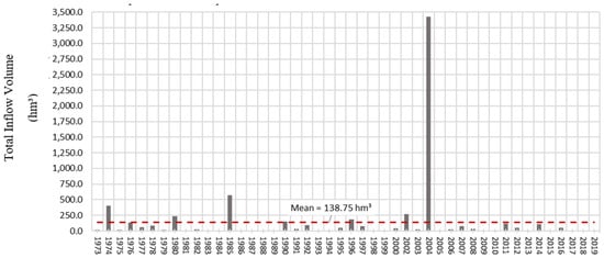
Figure 5.
Total flood volume in January and February at Jaguaribe River according to the river gauges station of Iguatu.
Therefore, this research seeks to study the flood events in this basin from an integrated perspective, considering both peak flows and volumes recorded during the event, based on a copula frequency analysis.
Two river gauge stations located in the main rivers that flow to Castanhão Dam were used to analyze the characteristics of these flood event. The Icó River gauge station is located at Rio Salgado, with a 12,000 km2 catchment, and the Iguatu River gauge station is located at Rio Jaguaribe, draining an area of 21,000 km2. Their historical data, starting in the year 1973, had missing records in 2001 that were not considered in the statistical analysis. With the daily flow records, it was possible to obtain the peak flow for each station, as shown in Figure 6.

Figure 6.
Flood peak from 1973 to 2019 for both river gauge stations.
Figure 6 indicates that both river gauge stations registered very high peak discharge in 1985. Additionally, high peak discharges also occurred in 2008 at the Icó station and in 2004 at the Iguatu station. The difference between the number of peak discharges at the two river gauge stations is justified by the difference in their drainage areas, in which Iguatu presents almost twice the area of the Iguatu station.
The second variable analyzed was the flood volume (Figure 7), defined as the volume from the beginning of each flood event until the time of occurrence of the respective peak flow. The volumes achieved show that 1974 and 1985 also stand out as the maximum values.

Figure 7.
Flood volume from 1973 to 2019 for both flow gauges.
The average flood intensity value in 2004 at Iguatu River gauge station is considerably above historical values (Figure 8). In hydrological terms, it can be understood that, during this event in 2004, there was a remarkable sequence of flows in a short time, causing runoff with maximum intensity given the conditions of complete soil saturation, and, therefore, minimal losses.

Figure 8.
Average flood intensity from 1973 to 2019 for both flow gauges.
The situation can be compared to flash flood events that may generate soil crusting. The areas next to the stream channels become saturated due to the shallow soils. Continuing rainfall causes the water table to rise to the ground surface, and the lower catchment slopes become saturated, with further rain flowing overland to the river channel. Runoff rates often far exceed those of other flood types due to the rapid response of the catchments to intense rainfall, modulated by soil moisture and soil hydraulic properties [,,,].
The same physical phenomenon defines flood peak, duration, and volume; thus, they should be mutually correlated []. The scatter plots between flood peak and average flood intensity and between flood peak and flood volume displayed in Figure 9 (illustrating data from the Iguatu River gauge) suggest the dependency between each two coupled variables. While Figure 9 specifically showcases the Iguatu station, similar strong correlations were also observed for the Icó River gauge, and these dependencies were comprehensively integrated into our subsequent bivariate frequency analysis for both stations. These results confirm a strong correlation between flood peak, volume, and duration, supporting the use of joint probabilistic models such as copulas in the subsequent analysis.

Figure 9.
Data correlation scatter plot Average Flood Intensity × Flood Peak and Flood Volume × Flood Peak (Iguatu River gauge). In the figure, C. stands for the Pearson Correlation Coefficient.
These results confirm a strong correlation between flood peak, volume, and duration, supporting the use of joint probabilistic models such as copulas in the subsequent analysis.
3.2. Frequency Analysis
To better comprehend the whole flood event, it is essential to understand the relationship among the variables previously defined. The analysis of the descriptive statistics of flood events (Table 1) showed in general that the coefficient of variation (CV) for all variables is higher at the Iguatu gauge. In other words, it has a high steepness of the flood frequency curve, since it is calculated as the standard deviation of the annual series divided by the mean.

Table 1.
Descriptive statistics of flood events for both flow gauges.
This CV can be considered a value well above the average of the world’s basins compared to the global perspective. High CVs may be due to nonlinear runoff generation processes, particularly threshold behavior, prevalent in semi-arid regions [].
3.2.1. Marginal Distribution
The distribution chosen for the work consists of the joint of average flood intensity (AFI) and flood peak, given that the main objective is to investigate the event of the year 2004, where the first variable has excellent prominence.
To ensure an objective and transparent selection of the marginal distributions, all six candidate models (Exponential, Gumbel, Gamma, Logistic, Lognormal, and Weibull) were fitted to the flood variables at both stations, and their performance was compared using the Akaike Information Criterion (AIC) and the Bayesian Information Criterion (BIC). Table 2 summarizes the results and Figure 10 shows an example of graphical visualization.
Table 2.
AIC and BIC values for all candidate marginal distributions tested at Iguatu and Icó River Gauge Station.

Figure 10.
Graphical visualization of marginal distributions tested for the average flood intensity of Iguatu River station.
For Iguatu (flood peak), the Weibull distribution achieved the lowest AIC (680.759), while the Exponential distribution yielded the lowest BIC (682.768). The visual diagnostics (Figure 10) indicate that both Weibull and Lognormal distributions approximate the empirical distribution reasonably well, but Weibull shows superior stability across the quantiles, corroborating its selection as the most suitable model.
For Iguatu (AFI), both AIC and BIC clearly identified the Weibull distribution as the best-fitting model (AIC = 1582.250; BIC = 1585.907), outperforming all other candidates by a substantial margin. This is consistent with the QQ and PP plots, which show the Weibull capturing the skewed behavior of the data more effectively than its competitors.
For Icó (flood peak), the Weibull distribution again provided the best fit according to both AIC (647.199) and BIC (650.856). However, the graphical diagnostics suggested that the Lognormal distribution also provides a reasonable approximation, especially in the right tail. This highlights the robustness of the Weibull fit, while also showing Lognormal as an acceptable alternative.
For Icó (AFI), both AIC and BIC clearly supported the Lognormal distribution (AIC = 1540.048; BIC = 1543.705). The visual analysis confirmed that Lognormal consistently outperformed the other candidates, particularly in aligning with the empirical quantiles in the central range, while Weibull and Gamma showed higher deviations.
Taken together, the combined evidence from information criteria and diagnostic plots supports the use of the Weibull distribution for both variables at Iguatu, and Weibull for flood peak and Lognormal for AFI at Icó. This comprehensive evaluation ensures that the marginal distributions employed in the copula modeling are not only statistically optimal but also visually consistent with the observed data.
3.2.2. Copula Function
The bivariate copulas were used to determine the best-fitted copula for modeling bivariate joint distribution between flow peaks and volumes, aiming at obtaining the corresponding joint return periods, which are essential for evaluating and predicting the regional flood magnitude. According to Section 3.1 and Section 3.2, one copula function was selected for each river gauge station.
The selection of copula families was based on the joint evaluation of AIC, BIC, and RMSE values (Table 3). For Iguatu, the Survival Gumbel copula provided the lowest AIC (−44.847) and BIC (−41.190), indicating the best overall performance among the candidate models. The standard Gumbel copula achieved the lowest RMSE (0.048), although the difference with the Survival Gumbel (0.052) was marginal. This suggests that, while both upper- and lower-tail dependencies are present, the lower-tail dependence captured by the Survival Gumbel dominates the dependence structure in Iguatu.
Table 3.
Copula model selection criteria (AIC, BIC, and RMSE) for candidate copula families fitted to the bivariate flood variables at Iguatu and Icó stations.
For Icó, the Survival Gumbel copula again achieved the best AIC (−39.037) and BIC (−35.380), while the Gaussian copula yielded the lowest RMSE (0.029), very close to the Survival Gumbel (0.030). This outcome suggests that the dependence structure in Icó is weaker and closer to symmetric, although the criteria still favor the Survival Gumbel, highlighting some degree of lower-tail dependence.
Overall, the results support the choice of the Survival Gumbel copula for both stations, with Iguatu showing stronger signs of asymmetric tail dependence, and Icó exhibiting a more balanced, nearly symmetric dependence structure.
3.2.3. Return Period
Table 4 and Figure 11 show the calculated return periods for the univariate and bivariate cases. In the context of bivariate return periods, two complementary definitions are commonly applied. The “or case” refers to the probability that at least one of the variables exceeds a given threshold (e.g., either flood peak or average flood intensity is extreme). This formulation represents a more conservative perspective, as it accounts for the occurrence of extremes in any of the two variables. In contrast, the “& case” corresponds to the probability that both variables simultaneously exceed their thresholds (flood peak and average flood intensity), which is a stricter criterion and results in larger return periods. Both definitions are reported here to provide a comprehensive picture of the joint flood hazard, following standard practice in copula-based hydrological frequency analysis.
Table 4.
Return period in years of flood peak and average flood intensity for univariate distribution. Joint flood peak or average flood intensity and flood peak and average flood intensity for the bivariate distribution.

Figure 11.
Return periods for flood peak or average flood intensity and flood peak and average flood intensity time series.
Overall, exceptionally rare events were identified in 1974, 1985, and 2004. In the univariate analysis, the average flood intensity observed in Iguatu in 2004 corresponds to a return period of approximately 584 years. However, when the joint copula-based model is applied, combining average flood intensity with flood peak, the estimated return period increases to nearly 995 years.
This striking difference illustrates how copula models provide a more comprehensive representation of the dependence structure between variables. While the univariate approach highlights the extremity of the 2004 event, the bivariate analysis reveals an even more exceptional return period, almost doubling the estimate from the single-variable case. These results confirm the added value of the copula approach in identifying extremely low-frequency hydrological events that cannot be adequately captured through univariate methods alone.
The results obtained from the bivariate analysis were compared with those from the univariate approach, revealing a clear informational gain when using the copula-based methodology. Figure 12 illustrates the percentage difference between the return periods estimated by the joint distribution and those derived from univariate analyses, whether based on peak flow or flood volume, for both gauging stations.

Figure 12.
Difference in percentual between the joint bivariate return periods against the univariate results.
In general, the higher the point on the graph, the greater the discrepancy between the two methods—indicating a potential underestimation of flood magnitude when relying solely on a single variable. Most of the observed differences range between 100% and 125%, suggesting that, for many years, the bivariate approach offers only moderate improvement over univariate models. However, for the most extreme events—namely, those in 1974, 1985, and 2004—the multivariate method proved particularly valuable, yielding substantially higher return periods.
The most pronounced difference was observed at the Icó station in 1985, where the return period estimated by the bivariate model reached 207.4 years, nearly 3.5 times higher than the 59.5 years estimated by the univariate analysis based on average flood intensity. Although not the most extreme case in this comparison, the year 2004 also showed a notably large divergence between the two approaches, reinforcing the importance of accounting for joint hydrological behavior in flood frequency analyses.
Figure 13 shows the comparison between the two basins and the ranking of the year’s events. The ranking (1 to 46) of the combined flood peak and average flood intensity events in each year was sorted in descending order, and its value was added for each flow gauge. The events in 1985 and 2004 are tied to the lowest classified years, which were the most extraordinary droughts identified in the region (1993, 1998, and 2013).

Figure 13.
Descending joint distribution return period ranking for annual events of flood peak and average flood intensity in both flow gauges.
4. Discussions and Conclusions
This study advances flood frequency analysis in semi-arid environments by introducing a copula-based bivariate framework that jointly models flood peak and average flood intensity (AFI). The inclusion of AFI—a variable designed to capture the rapid runoff and high-volume dynamics typical of intermittent rivers—represents a conceptual contribution that complements traditional flood peak analysis. This refinement is especially relevant in semi-arid regions such as Northeast Brazil, where short concentration times and flashy hydrological responses amplify flood hazards.
The case of the 2004 flood in Iguatu illustrates the added value of this approach. While univariate analysis estimated a return period of only 35 years for the flood peak, the copula-based bivariate model revealed a joint return period of nearly 995 years when AFI was considered together with flood peak. Although such extrapolations must be interpreted with caution, this striking difference demonstrates how univariate models can severely underestimate compound flood hazard. More broadly, our findings align with and extend prior studies that highlighted the limitations of univariate approaches (e.g., Villarini and Smith, []) by showing that dependence between flood characteristics must be explicitly accounted for to capture the true rarity of extreme events.
The practical implications are substantial. In the Brazilian Semi-Arid, large hydraulic infrastructures such as the Castanhão Reservoir are central to water security and socio-economic stability. Accurate estimation of flood return periods is therefore critical for dam design, safety assessments, and operational decision making. By improving the reliability of flood frequency analysis, the proposed copula framework provides a replicable methodology for risk-informed management in data-scarce and climatically variable regions, providing actionable information for climate adaptation, such as adaptive rule curves and risk screening techniques.
Despite these advances, important limitations remain. The 46-year observation record restricts the robustness of estimates for return periods on the order of centuries or millennia, as demonstrated by the wide uncertainty surrounding the 2004 event. Confidence intervals were not explicitly quantified here, but future studies should formally incorporate bootstrap or parametric approaches to assess the statistical uncertainty of extreme-value extrapolations. Another limitation arises from the intrinsic dependence between flood peak and AFI, which reduces the effective number of independent observations. Nevertheless, this dependence underscores the need for multivariate modeling, as copula functions offer a flexible means to represent asymmetric tail dependencies that univariate methods systematically overlook.
Future research should aim to expand the framework in three directions. First, by incorporating additional hydrological variables such as antecedent soil moisture, which can influence both flood generation and impacts. Second, by testing a broader range of copula families and tail dependence structures under different hydrological regimes so to assess the robustness of the approach. Third, by exploring the integration of this methodology into operational flood forecasting and dam management systems, thereby translating probabilistic modeling into actionable decision support tools.
In summary, the copula-based bivariate framework presented here contributes to both theory and practice by enhancing the representation of compound flood events. It reveals hidden exceptionality in historical floods, improves the scientific basis for infrastructure design and flood risk management, and opens new pathways for research into probabilistic hydrology in semi-arid and data-limited environments.
Author Contributions
Conceptualization, T.M.C.S. and M.M.P.; methodology, T.M.C.S., J.D.P.F. and G.R.G.; software, J.D.P.F. and G.R.G.; validation, J.D.P.F., T.M.C.S. and F.A.S.F.; formal analysis, J.D.P.F. and G.R.G.; resources, T.M.C.S.; data curation, G.R.G.; writing—original draft preparation, T.M.C.S. and G.R.G.; writing—review and editing, J.D.P.F. and T.M.C.S.; visualization, G.R.G.; supervision, T.M.C.S. and F.A.S.F.; project administration, T.M.C.S.; funding acquisition, T.M.C.S. All authors have read and agreed to the published version of the manuscript.
Funding
This research was funded by Fundação Cearense de Apoio ao Desenvolvimento Científico e Tecnológico (FUNCAP), grant number UNI-0210-00316.01.00/23.
Data Availability Statement
The datasets presented in this article are not readily available because they are provided by other institutions upon request. Requests to access the datasets should be directed to the authors to understand demand.
Acknowledgments
The first author would like to thank the National Council for Scientific and Technological Development (CNPq) for the grant number 314861/2023-8. During the preparation of this manuscript, the authors used ChatGPT 5.0 for the purposes of language refinement, including English grammar review, vocabulary enhancement, and improvement of textual fluency. The authors have reviewed and edited the output and take full responsibility for the content of this publication.
Conflicts of Interest
The authors declare no conflicts of interest. The funder had no role in the design of the study; in the collection, analyses, or interpretation of data; in the writing of the manuscript; or in the decision to publish the results.
References
- Yin, J.; Gao, Y.; Chen, R.; Yu, D.; Wilby, R.; Wright, N.; Ge, Y.; Bricker, J.; Gong, H.; Guan, M. Flash Floods: Why Are More of Them Devastating the World’s Driest Regions? Setting the Agenda in Research. Nature 2023, 615, 212–215. [Google Scholar] [CrossRef]
- Nabinejad, S.; Schüttrumpf, H. Flood Risk Management in Arid and Semi-Arid Areas: A Comprehensive Review of Challenges, Needs, and Opportunities. Water 2023, 15, 3113. [Google Scholar] [CrossRef]
- Villarini, G.; Smith, J.A. Flood Peak Distributions for the Eastern United States. Water Resour. Res. 2010, 46. [Google Scholar] [CrossRef]
- Calenda, G.; Mancini, C.P.; Volpi, E. Distribution of the Extreme Peak Floods of the Tiber River from the XV Century. Adv. Water Resour. 2005, 28, 615–625. [Google Scholar] [CrossRef]
- Karmakar, S.; Simonovic, S.P. Bivariate Flood Frequency Analysis: Part 1. Determination of Marginals by Parametric and Nonparametric Techniques. J. Flood Risk Manag. 2008, 1, 190–200. [Google Scholar] [CrossRef]
- Shiau, J.T. Fitting Drought Duration and Severity with Two-Dimensional Copulas. Water Resour. Manag. 2006, 20, 795–815. [Google Scholar] [CrossRef]
- Alidoost, F.; Su, Z.; Stein, A. Evaluating the Effects of Climate Extremes on Crop Yield, Production and Price Using Multivariate Distributions: A New Copula Application. Weather Clim. Extrem. 2019, 26, 100227. [Google Scholar] [CrossRef]
- Filho, J.P.; Portela, M.; Studart, T.; Souza Filho, F. A Continuous Drought Risk Monitoring System, CDRMS, Based on Copulas. In Water: Ecology and Management; Vide Leaf: Hyderabad, India, 2020; pp. 1–31. [Google Scholar]
- Xu, K.; Yang, D.; Xu, X.; Lei, H. Copula Based Drought Frequency Analysis Considering the Spatio-Temporal Variability in Southwest China. J. Hydrol. 2015, 527, 630–640. [Google Scholar] [CrossRef]
- Genest, C.; Favre, A.-C. Everything You Always Wanted to Know about Copula Modeling but Were Afraid to Ask. J. Hydrol. Eng. 2007, 12, 347–368. [Google Scholar] [CrossRef]
- Zhang, L.; Singh, V.P. Bivariate Rainfall Frequency Distributions Using Archimedean Copulas. J. Hydrol. 2007, 332, 93–109. [Google Scholar] [CrossRef]
- Favre, A.C.; Adlouni, S.E.; Perreault, L.; Thiémonge, N.; Bobée, B. Multivariate Hydrological Frequency Analysis Using Copulas. Water Resour. Res. 2004, 40. [Google Scholar] [CrossRef]
- Gaál, L.; Szolgay, J.; Kohnová, S.; Hlavčová, K.; Parajka, J.; Viglione, A.; Merz, R.; Blöschl, G. Relation Entre Pics et Volumes de Crues: Étude Des Déterminants Climatiques et Hydrologiques. Hydrol. Sci. J. 2015, 60, 968–984. [Google Scholar] [CrossRef]
- Pontes Filho, J.D.; Souza Filho, F.d.A.; Martins, E.S.P.R.; Studart, T.M.d.C. Copula-Based Multivariate Frequency Analysis of the 2012–2018 Drought in Northeast Brazil. Water 2020, 12, 834. [Google Scholar] [CrossRef]
- Mirabbasi, R.; Fakheri-Fard, A.; Dinpashoh, Y. Bivariate Drought Frequency Analysis Using the Copula Method. Theor. Appl. Climatol. 2012, 108, 191–206. [Google Scholar] [CrossRef]
- De Michele, C.; Salvadori, G.; Canossi, M.; Petaccia, A.; Rosso, R. Bivariate Statistical Approach to Check Adequacy of Dam Spillway. J. Hydrol. Eng. 2005, 10, 50–57. [Google Scholar] [CrossRef]
- Bockheim, J.G. Classification and Development of Shallow Soils (<50cm) in the USA. Geoderma Reg. 2015, 6, 31–39. [Google Scholar] [CrossRef]
- Campos, J.N.B. Paradigms and Public Policies on Drought in Northeast Brazil: A Historical Perspective. Environ. Manag. 2015, 55, 1052–1063. [Google Scholar] [CrossRef]
- Silva, B.K.N.; Amorim, A.C.B.; Silva, C.M.S.; Lucio, P.S.; Barbosa, L.M. Rainfall-Related Natural Disasters in the Northeast of Brazil as a Response to Ocean-Atmosphere Interaction. Theor. Appl. Climatol. 2019, 138, 1821–1829. [Google Scholar] [CrossRef]
- Delgado, J.M.; Voß, S.; Bürger, G.; Vormoor, K.; Murawski, A.; Pereira, J.M.R.; Martins, E.; Vasconcelos Júnior, F.; Francke, T. Seasonal Drought Prediction for Semiarid Northeastern Brazil: Verification of Six Hydro-Meteorological Forecast Products. Hydrol. Earth Syst. Sci. 2018, 22, 5041–5056. [Google Scholar] [CrossRef]
- Stefan Hastenrath, B.; Heller, L. Dynamics of Climatic Hazards in Northeast Brazil. Q. J. R. Meteorol. Soc. 1977, 103, 77–92. [Google Scholar] [CrossRef]
- Hastenrath, S. Exploring the Climate Problems of Brazil’s Nordeste: A Review. Clim. Chang. 2012, 112, 243–251. [Google Scholar] [CrossRef]
- Uvo, C.B.; Repelli, C.A.; Zebiak, S.E.; Kushnir, Y. The Relationships between Tropical Pacific and Atlantic SST AndNortheast Brazil Monthly Precipitation. J. Clim. 1998, 11, 551–562. [Google Scholar] [CrossRef]
- U.S. Department of the Interior Bureau of Reclamation. Design Standards No. 13 Dams; U.S. Department of the Interior Bureau of Reclamation: Washington, DC, USA, 2014.
- International Commission on Large Dams-Commission Internationale Des Grands Barrages. Dam Surveillance Lessons Learnt from Case Histories; International Commission on Large Dams-Commission Internationale Des Grands Barrages: Chatou, France, 2017. [Google Scholar]
- Du, É.; Dans, R.; De, L.G.; Sécurité, L.A.; Barrage, D.U. Risk Assessment in Dam Safety Management A Reconnaissance of Benefits, Methods and Current Applications; Association of State Dam Safety Officials: Lexington, KY, USA, 2005. [Google Scholar]
- Dam Safety Guidelines 2007; Canadian Dam Association: Markham, ON, Canada, 2013; ISBN 9780993631900.
- Guru, N.; Jha, R. Flood Frequency Analysis of Tel Basin of Mahanadi River System, India Using Annual Maximum and POT Flood Data. Aquat. Procedia 2015, 4, 427–434. [Google Scholar] [CrossRef]
- Papaioannou, G.; Kohnová, S.; Bacigál, T.; Szolgay, J.; Hlavčová, K.; Loukas, A. Joint Modelling of Flood Peaks and Volumes: A Copula Application for the Danube River. J. Hydrol. Hydromech. 2016, 64, 382–392. [Google Scholar] [CrossRef]
- Joe, H. Multivariate Models and Dependence Concepts; Chapman & Hall: London, UK, 1997. [Google Scholar]
- Brechmann, E.C.; Schepsmeier, U. Modeling Dependence with C- and D-Vine Copulas: The R Package CDVine. J. Stat. Softw. 2013, 52, 1–27. [Google Scholar] [CrossRef]
- Zehe, E.; Blöschl, G. Predictability of Hydrologic Response at the Plot and Catchment Scales: Role of Initial Conditions. Water Resour. Res. 2004, 40. [Google Scholar] [CrossRef]
- Brabo Alves, J.M.; Ferreira, F.F.; Campos, J.N.B.; De, F.; De, A.; Filho, S.; De Souza, E.B.; Duran, B.J.; Servain, J.; Studart, T.M.C. Mecanismos Atmosféricos Associados à Ocorrência de Precipitação Intensa Sobre o Nordeste do Brasil Durante Janeiro/2004. Rev. Bras. De Meteorol. 2006, 21, 56–76. [Google Scholar]
- Borga, M.; Anagnostou, E.N.; Blöschl, G.; Creutin, J.D. Flash Flood Forecasting, Warning and Risk Management: The HYDRATE Project. Environ. Sci. Policy 2011, 14, 834–844. [Google Scholar] [CrossRef]
- Collier, C.G. Flash Flood Forecasting: What Are the Limits of Predictability? Q. J. R. Meteorol. Soc. 2007, 133, 3–23. [Google Scholar] [CrossRef]
- Hardy, J.; Gourley, J.J.; Kirstetter, P.E.; Hong, Y.; Kong, F.; Flamig, Z.L. A Method for Probabilistic Flash Flood Forecasting. J. Hydrol. 2016, 541, 480–494. [Google Scholar] [CrossRef]
- Ruiz-Villanueva, V.; Borga, M.; Zoccatelli, D.; Marchi, L.; Gaume, E.; Ehret, U. Extreme Flood Response to Short-Duration Convective Rainfall in South-West Germany. Hydrol. Earth Syst. Sci. 2012, 16, 1543–1559. [Google Scholar] [CrossRef]
- Grimaldi, S.; Serinaldi, F. Asymmetric Copula in Multivariate Flood Frequency Analysis. Adv. Water Resour. 2006, 29, 1155–1167. [Google Scholar] [CrossRef]
- Chen, J.; Wu, X.; Finlayson, B.L.; Webber, M.; Wei, T.; Li, M.; Chen, Z. Variability and Trend in the Hydrology of the Yangtze River, China: Annual Precipitation and Runoff. J. Hydrol. 2014, 513, 403–412. [Google Scholar] [CrossRef]
Disclaimer/Publisher’s Note: The statements, opinions and data contained in all publications are solely those of the individual author(s) and contributor(s) and not of MDPI and/or the editor(s). MDPI and/or the editor(s) disclaim responsibility for any injury to people or property resulting from any ideas, methods, instructions or products referred to in the content. |
© 2025 by the authors. Licensee MDPI, Basel, Switzerland. This article is an open access article distributed under the terms and conditions of the Creative Commons Attribution (CC BY) license (https://creativecommons.org/licenses/by/4.0/).