Groundwater Level Estimation Using Improved Transformer Model: A Case Study of the Yellow River Basin

Abstract

Accurate estimation of groundwater levels in river basins is essential for effective water resource planning. Innovations in deep learning and artificial intelligence (AI) have been introduced into this field to enhance the accuracy of long-term groundwater level estimation. This study employs the Transformer deep learning model to estimate groundwater levels, with a benchmark comparison against the long short-term memory (LSTM) model. These models were applied to estimate groundwater levels in the Yellow River Basin, where approximately 1100 monitoring wells are located. Monthly average groundwater level data from the period 2018–2023 were collected from these wells. The two models were used to estimate groundwater levels for the period 2003–2017 by incorporating remote sensing information. The Transformer model was enhanced to simultaneously capture features from both historical temporal data and surrounding spatial data, while automatically enhancing key features, effectively improving estimation accuracy and robustness. At the basin-averaged scale, the enhanced Transformer model outperformed the LSTM model: R² increased by approximately 17.5%, while RMSE and MAE decreased by approximately 12.4% and 10.9%, respectively. The proportion of poorly predicted samples decreased by an average of approximately 12.1%. The estimation model established in this study contributes to improving the quantitative analysis capability of long-term groundwater level variations in the Yellow River Basin. This could be helpful for water resource development planning in this densely populated region and likely has broad applicability in other river basins.

1. Introduction

Groundwater constitutes a critical global water resource, providing drinking water to approximately half of the world’s population [1] and supporting around 33% of global irrigation water demand [2]. However, driven by continuous population growth and exacerbated by climate change [3], unsustainable groundwater over-extraction has emerged as a widespread phenomenon. This leads to the rapid depletion of groundwater resources in many regions worldwide, surpassing anticipated rates [4], thereby posing a severe threat to both human societal development and natural ecosystem protection. Consequently, accurately assessing the dynamic trends of groundwater storage changes becomes essential for ensuring water security and achieving regional sustainable development.

Groundwater monitoring has traditionally relied on in situ measurement methods, such as monitoring wells [5]. But these approaches entail substantial labor and equipment costs and exhibit limited spatial and temporal coverage, presenting significant challenges for acquiring continuous, long-term groundwater level data across large regional scales. Within this context, remote sensing technologies offer a critical alternative. Current satellite systems, including GRACE/GRACE-FO [6], GLDAS, SMAP, and NISAR, have demonstrated substantial utility for groundwater level estimation and hold promise for broad application.

Groundwater level estimation primarily relies on two types of methods: physical models and data-driven models. Physical models are typically based on the groundwater-subsidence coupling theory [7], the groundwater–surface water hydrological coupling theory [8], or the Darcy’s law–mass conservation law coupling model [9]. These models require a large amount of precise hydrological observation data for parameter calibration to ensure the reliability of the simulation results. However, physical models face significant challenges: the required hydrological parameters are diverse and demand high accuracy, and their calibration process involves complex reasoning and iterative calculations [10]. Additionally, uncertainties inherent in the physical models, such as the choice of parameter types and boundary condition settings, can significantly constrain the interpretability of the estimation results [11].

Machine learning methods, particularly deep learning techniques, have demonstrated significant utility in time series estimation tasks in recent years [12]. Among these, long short-term memory (LSTM) networks utilize gating mechanisms to selectively retain or discard information, enabling effective capture of temporal dependencies within extended sequences. This capability has established LSTM as a widely applied approach for groundwater level estimation; researchers have successfully employed it using actual monitoring data [13]. But LSTM exhibits notable limitations in modeling long-term temporal dependencies: its relatively simple gating architecture is susceptible to challenges such as vanishing or exploding gradients [14]. Furthermore, its performance is constrained in scenarios characterized by severe data sparsity or sequences exhibiting strong nonlinearity.

The Transformer model is a deep learning architecture based on the self-attention mechanism [15], which abandons the traditional Recurrent Neural Network (RNN) and Convolutional Neural Network (CNN) structures, instead adopting a multi-head self-attention mechanism to capture global dependencies between arbitrary elements in the input sequence, particularly excelling at processing long sequence data. This model has been widely applied in the field of Natural Language Processing (NLP) for tasks such as machine translation, text generation, and question answering systems [16]. In recent years, its powerful self-attention mechanism has attracted the attention of time series estimation researchers [17]. Researchers treat time series as sequential data and utilize the Transformer to capture complex long-term patterns and correlations within the sequence. These explorations have demonstrated the potential of the Transformer in handling complex long-sequence time prediction tasks. Moreover, the successful applications of Transformer in hydrology, meteorology, and other earth science fields [18,19] further indicate its applicability to groundwater level estimation tasks. This study aims to leverage the advantages of the Transformer model in complex time series modeling, particularly its strong representation capability of long-sequence temporal features through the self-attention mechanism, with the goal of improving groundwater level estimation accuracy and exploring its new application value beyond traditional fields such as Natural Language Processing.

The Transformer model serves as the foundational architecture for this study. To address specific characteristics of groundwater level estimation, we implement the following enhancements. Groundwater level fluctuations are governed by both temporal variations within the local region and hydrological interactions with surrounding areas [20], but previous studies on groundwater time series estimation have predominantly focused on local temporal dynamics [21], with limited incorporation of spatial interdependencies between regions. This limitation may particularly impact areas characterized by sparse observation points.

To effectively integrate information from surrounding regions into the estimation process, we propose a Dynamic–Static Feature Fusion (DSFF) mechanism tailored for the Transformer architecture. This mechanism utilizes the contextual relationships between input keys to guide the learning of a dynamic attention matrix, thereby capturing intrinsic temporal dependencies within the target region. Concurrently, a 3 × 3 convolutional layer extracts static spatial–contextual information from adjacent areas. The fused static and dynamic contextual representations subsequently serve as the input for modeling. This enhancement successfully augments the model’s information acquisition capability.

Groundwater level variations are governed by multiple driving factors, with dominant influences and their relative contributions exhibiting significant spatial heterogeneity [22]. While prior studies have addressed factor influence, they predominantly employed correlation analyses of input hydrological features (e.g., Pearson’s correlation coefficient) [23], providing relatively limited insight into the dynamic weight allocation mechanisms within temporal feature representations. This inherent constraint fundamentally restricts model interpretability during estimation.

Consequently, when applying the Transformer architecture for groundwater level estimation, the dynamic evaluation and utilization of feature channel weights constitutes a critical challenge. To address this, we design a Key Feature Enhancement Architecture (KFEA) tailored for the Transformer model, explicitly modeling inter-channel dependencies and integrating the squeeze-and-excitation (SE) mechanism to generate pixel-specific channel weights. This mechanism adaptively enhances feature channels, conveying information-rich signals while suppressing those containing redundant or less relevant information. This selective emphasis enables the model to concentrate on the most critical temporal patterns during estimation, thereby substantially enhancing the interpretability of the estimation process.

This study addresses three principal challenges in large-scale groundwater time series estimation: the inadequate modeling of long-range temporal dependencies, imprecise identification of critical temporal features, and insufficient incorporation of spatiotemporal information correlation. To overcome these limitations, we propose a groundwater level estimation model founded on an enhanced Transformer architecture. Our core contributions are summarized as follows: (1) We introduce a Transformer encoder framework for time series estimation, which employs sliding windows to extract local temporal features, self-attention mechanisms to capture global dependencies, and positional encoding to preserve temporal integrity. This approach enhances the model’s capacity to represent long-range dependencies. (2) The KFEA dynamically calibrates feature channel weights via squeeze-and-excitation (SE) operations, adaptively amplifying information-rich channels and suppressing noise, thus improving sensitivity to critical features and robustness against anomalies. (3) The DSFF mechanism integrates the target pixel’s dynamic temporal features with adjacent pixels’ static spatial contexts using a 3 × 3 convolutional layer, addressing spatiotemporal correlation challenges and enhancing spatial consistency of estimation results.

2. Materials and Methods

2.1. Study Area

The study area encompasses the Yellow River Basin (32° N–42° N, 96° E–119° E), spanning approximately 795,000 km² (Figure 1). This basin traverses the Qinghai–Tibet Plateau, Loess Plateau, Inner Mongolia Plateau, and North China Plain, exhibiting complex topographical gradients across China’s three major geomorphological steps. Climatically, the basin is characterized by a mean annual temperature of 5.8 °C, mean annual precipitation of 466.5 mm, and potential evapotranspiration of 653.6 mm [24], based on long-term observational records. Groundwater constitutes a critical component of the basin’s hydrological cycle, regulating regional water resource dynamics. However, comprehensive basin-scale assessment is challenged by spatially heterogeneous groundwater monitoring infrastructure, with significant regions exhibiting sparse or nonexistent well observation points [25]. This constraint necessitates the development of novel data acquisition approaches to support quantitative groundwater resource evaluation.

2.2. Data Sources

2.2.1. The Gravity Recovery and Climate Experiment (GRACE)

The GRACE mission (National Aeronautics and Space Administration (NASA), Washington, DC, USA) provides a methodology for monitoring large-scale mass variations within the Earth system. Utilizing a twin-satellite ranging system, GRACE observes the Earth’s mass distribution and transport dynamics, enabling estimation of terrestrial water storage changes—comprising snow water equivalent, surface water, soil moisture, and groundwater storage. The derived GRACE dataset quantifies terrestrial water storage anomalies as equivalent water height (EWH). An eleven-month observational gap exists between the conclusion of GRACE operations and the initiation of GRACE Follow-On (GRACE-FO). To meet the needs of remote sensing data for groundwater level in the model training parts and inversion estimation parts must ensure data continuity, missing monthly EWH values within this gap were reconstructed using cubic spline interpolation, resulting in a continuous terrestrial water storage time series from April 2003 to October 2023 [26].

2.2.2. Global Land Data Assimilation System (GLDAS)

The GLDAS soil moisture dataset, collaboratively developed by NASA and the National Oceanic and Atmospheric Administration (NOAA), leverages land surface modeling frameworks and data assimilation methodologies. This integration merges satellite remote sensing observations with in situ ground-based measurements to enable precise estimations of land surface flux dynamics and state variable distributions. For the present study, we utilize the 2 m depth soil moisture outputs from the GLDAS Noah-V2.1 model to characterize the spatiotemporal patterns of soil water storage within the Yellow River Basin.

2.2.3. Measured Groundwater Level

The groundwater level data used in this study are provided by the China Geological Environmental Monitoring Institute (Geological Cloud 3.0, cgs.gov.cn), which are obtained from observation wells (approximately 1100) in certain regions of the Yellow River Basin. The data covers the period from October 2018 to October 2023 at monthly intervals, with high precision. The well observation points are mainly distributed in plains, river valleys, and other areas with high human activity (Figure 1).

2.3. Methods

2.3.1. Calculation Method of Groundwater Level

Observing and quantifying groundwater level variations presents significant challenges, especially in large aquifer systems [27]. Direct measurements of groundwater levels depend on a network of observation wells with sparse spatial distribution, which often lacks the spatial coverage required to resolve aquifer heterogeneity. Consequently, large-scale groundwater level monitoring necessitates the integration of remote sensing data with in situ measurements to enable the estimation of groundwater level over extensive areas.

In the estimation of groundwater level from remote sensing data, the conversion of GRACE terrestrial water storage to groundwater storage is essential. Current methodologies primarily include the mass balance equation approach [28,29,30,31], lithology method [32], and filtering technique [33]. The mass balance equation, the most widely adopted approach, quantifies total mass or water volume changes within time-varying gravitational fields by integrating complementary hydrological datasets to derive target variables [34]. Its clear physical basis has enabled frequent applications in groundwater storage estimation and assessments of extreme climatic events (e.g., droughts and floods) [35]. This study employs the mass balance equation method for analytical purposes, leveraging its rigorous framework to resolve groundwater storage from GRACE-derived terrestrial water storage signals, and the groundwater storage and groundwater level well observation values are modeled for time series estimation.

The mass balance equation represents the influence of factors such as soil water, snowmelt, and surface water [36].

$$\mathsf{\Delta }GWS=\mathsf{\Delta }TWS-\mathsf{\Delta }SWS-\mathsf{\Delta }SMS$$

(1)

In the equation, ΔGWS, ΔTWS, ΔSWS, and ΔSMS denote the anomalies of groundwater storage change, total water storage change, surface water storage change, and soil moisture storage change, respectively, during the study period (cm). GRACE satellite data are typically employed to characterize the total water storage change (ΔTWS), whereas GLDAS soil moisture data represent the soil moisture storage change (ΔSMS). The surface water storage change (ΔSWS) is often omitted in groundwater storage estimation, as groundwater constitutes over 90% of the Earth’s total liquid freshwater resources [37,38]. Groundwater storage quantifies the vertical water change, while surface water storage reflects horizontal water movement. The vertical component of surface water storage change is generally negligible compared to its horizontal counterpart [39].

2.3.2. Spatial Interpolation Methods

The highest-resolution remote sensing data used in this study is the 0.25° GLDAS-2 dataset. Therefore, other datasets in this research underwent spatial interpolation or resampling to uniformly align with the 0.25° × 0.25° grid of GLDAS, covering a total of 1277 pixels across the Yellow River Basin.

1.

Inverse Distance Weighting

Inverse distance weighting (IDW) represents a deterministic interpolation approach rooted in distance-weighting principles. Its core premise is that proximal data points exert a greater influence on the predicted value, with the impact of distant points diminishing monotonically with increasing spatial separation. The IDW formulation employs a weighted average framework, where the assigned weights are inversely proportional to the distance raised to a power (commonly set to (p = 2)). This method eschews reliance on statistical modeling, featuring a computationally parsimonious architecture that facilitates straightforward implementation, thereby rendering it suitable for rapid generation of smooth spatial distributions. For the present study, a K-nearest neighbor (K-NN) variant of IDW is adopted to enhance computational efficiency and mitigate the influence of remote data points. This is achieved by imposing a constraint on the number of neighboring points included in the interpolation calculation. Through systematic accuracy comparisons, the optimal K value is determined to be 10, striking a balance between computational tractability and spatial interpolation fidelity.

2.

Ordinary Kriging

Kriging interpolation is a statistical-based spatial interpolation method assuming geographic data have spatial autocorrelation, which is quantified by a variogram. This method provides not only predicted values but also prediction error estimates, making it suitable for variables with spatial continuity. The values at unknown points are calculated by computing the experimental variogram, fitting a theoretical variogram model (spherical model in this study), and using the Linear Unbiased Estimation (BLUE) method. Compared with simpler interpolation methods, Kriging interpolation handles uneven data distributions more effectively. However, it has higher computational complexity and is sensitive to the choice of variogram model.

2.3.3. Machine Learning Methods

In this study, we utilized machine learning methods to integrate ground well data with remote sensing data for estimating groundwater levels. Ground well data provide direct measurements of actual groundwater levels but suffer from short temporal coverage and uneven spatial distribution, while remote sensing data capture groundwater storage anomalies with longer temporal records and broad spatial coverage. A physical relationship exists between these two datasets, and this relationship function remains relatively stable over time at any given pixel location. Therefore, we employed machine learning methods to analyze the relationship between these datasets at each pixel and subsequently used this to estimate groundwater levels for years lacking actual well measurements.

Our study period was divided into a ‘Model Training Period’ and a ‘Retrieval Estimation Period’: the Model Training Period spanned from October 2018 to October 2023. During this period, both ground well data and remote sensing data were available. Various machine learning models, as will be introduced later, were trained 200 times on the data for each pixel within this period to obtain the optimal training results. The Retrieval Estimation Period covered April 2003 to September 2018. For this period, only remote sensing data were available. The optimal relationships derived during the Model Training Period were applied to the remote sensing data from the Retrieval Estimation Period to estimate the actual groundwater levels.

1.

Transformer model

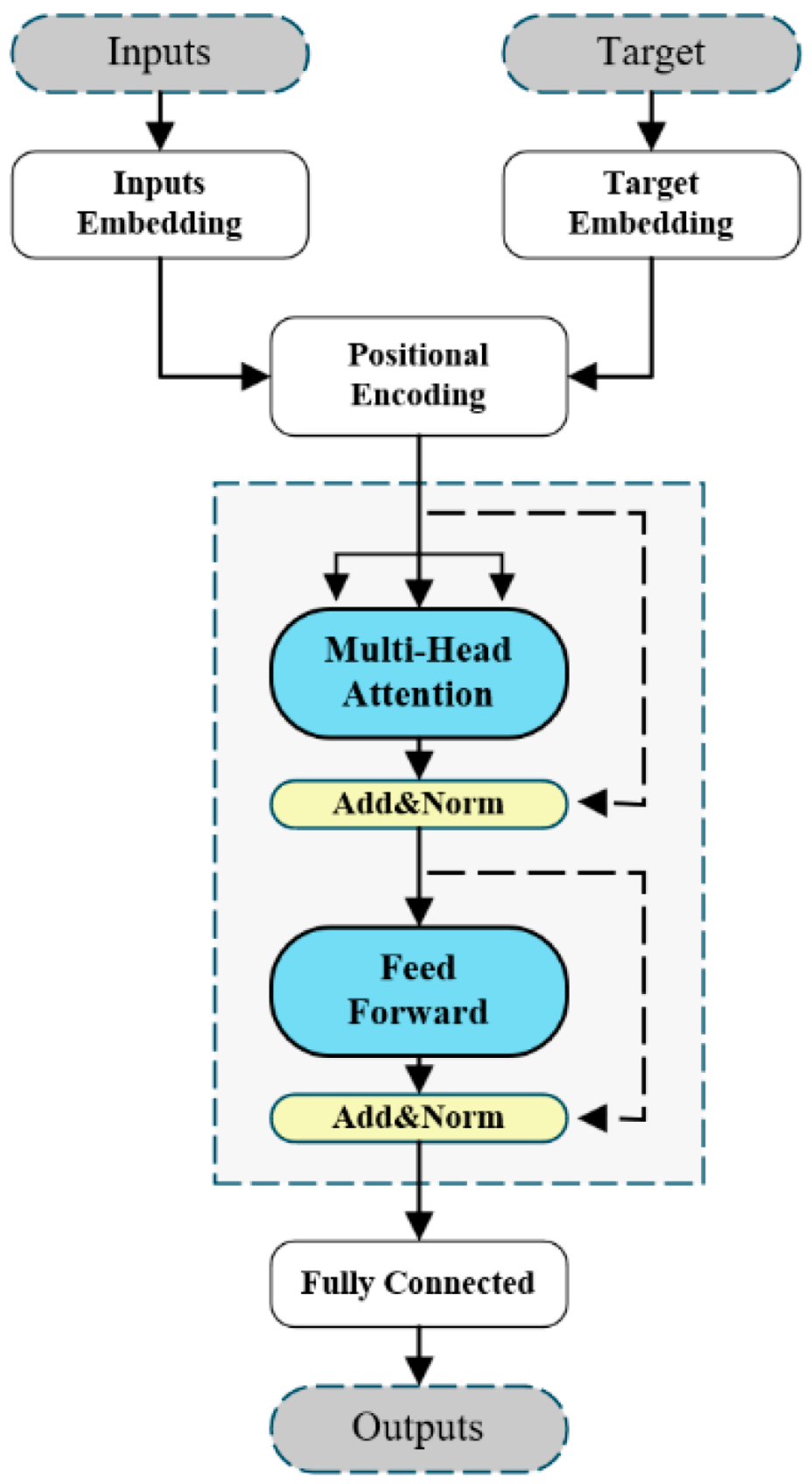
The main structure of the time series forecasting Transformer model consists of a linear embedding layer, a positional encoding layer, Transformer encoder layers, and a fully connected layer (Figure 2).

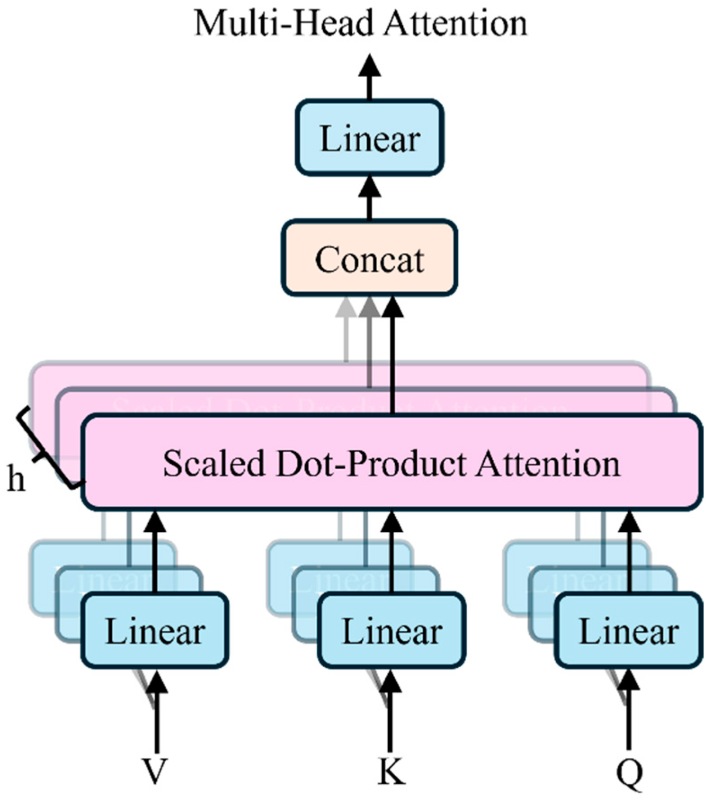
The Transformer encoder layer serves as the core of the entire model, undertaking the critical tasks of time series feature extraction and feature representation learning. Composed of multiple identical encoder sub-layers, each sub-layer consists of a multi-head self-attention layer and a feedforward neural network layer. The multi-head self-attention layer enables the model to focus on information from different positions within the input sequence during processing; by utilizing input query, key, and value matrices to compute attention scores, the attention results from multiple heads are concatenated and linearly transformed to generate the final output (Figure 3). This mechanism allows the model to capture input sequence information from different representation subspaces, thereby enhancing both its expressive and generalization capabilities.

$$\mathrm{Mu}\mathrm{l}\mathrm{ti}\text{-}\mathrm{Head}(\mathrm{Q},\mathrm{K},\mathrm{V})=\mathrm{Concat}\left({\mathrm{head}}_1,{\mathrm{head}}_2,\dots ,{\mathrm{head}}_{\mathrm{h}}\right){\mathrm{W}}^0$$

(2)

$${\mathrm{head}}_{\mathrm{i}}=\mathrm{Attention}\left(\mathrm{Q}{\mathrm{W}}_{\mathrm{i}}^{\mathrm{Q}},\mathrm{K}{\mathrm{W}}_{\mathrm{i}}^{\mathrm{K}},\mathrm{V}{\mathrm{W}}_{\mathrm{i}}^{\mathrm{V}}\right)$$

(3)

In the self-attention mechanism, Q (query), K (key), and V (value) are essential components. The query represents the information request from each input position, allowing the model to search for information from other positions. The key identifies the information associated with each input position, assisting in matching with the query to find relevant positions. The value contains the actual information associated with the key, which, once a match is found, is used for computation and output generation.

The feedforward network (FFN) performs nonlinear transformations and feature extraction on the output of the multi-head self-attention mechanism, followed by residual connections and normalization operations.

The linear embedding layer maps the input data from the original low-dimensional space to a higher-dimensional feature space, thereby providing a richer feature representation.

The positional encoding layer generates a unique encoding vector for each position in the input sequence and adds this vector to the input embedding vector at that position, enabling the Transformer model to distinguish elements at different positions when processing the input data. The positional encoding vectors are generated by a combination of sine and cosine functions, with each dimension corresponding to a different frequency. The positional encoding model is computed as follows:

$$\mathrm{P}{\mathrm{E}}_{(\mathrm{pos},2\mathrm{i})}=\sin \left({\displaystyle \frac{\mathrm{pos}}{\mathrm{10,000}\frac{2\mathrm{i}}{{\mathrm{d}}_{\mathrm{model}}}}}\right)$$

(4)

$$\mathrm{P}{\mathrm{E}}_{(\mathrm{pos},2\mathrm{i}+1)}=\cos \left({\displaystyle \frac{\mathrm{pos}}{\mathrm{10,000}\frac{2\mathrm{i}}{{\mathrm{d}}_{\mathrm{model}}}}}\right)$$

(5)

Here, PE denotes the positional encoding matrix obtained through the positional encoding operation, where (i) represents the dimension index, (pos) represents the position index, and $d_{\mathrm{model}}$ represents the input dimensionality.

The time series prediction process of Transformer model can be roughly described as follows, as shown in Figure 4a, predicting the future time point dataset with the past time series data (estimation in this paper). Different combinations of solid lines represent different sample learning strategies. The red dashed line on the right in the figure represents the predicted object for this step, and self-represents the input for this step.

To grasp the relationship between long-term dependence and short-term dependence on data, different “layers” pay different attention to different time series patterns. Figure 5 shows the attention patterns of several layers. For example, some layers focus on the most recent month and give the highest weight to these months (Figure 5: red line); some layers focus on long-term periodicity and give higher weight to the similar months of each year (Figure 5: green line); while some layers have no obvious tendency and give uniform weight to the data of each month (Figure 5: yellow line); and some layers attend from near to far, taking into account the short-term and long-term characteristics (Figure 5: blue line). The set meaning is shown in Figure 4b–d, where the purple input is the high-weight object. By stacking multiple self-attention layers and applying appropriate methods to determine the importance of different layers later, we obtain the final estimation result.

2.

Key Feature Enhancement Architecture

In large-scale groundwater estimation, abnormal time series induced by extreme hydrological events yield fluctuations with characteristics inconsistent with actual well observations. To address this, a Key Feature Enhancement Architecture (KFEA) based on SE-Net (squeeze-and-excitation networks) is designed in this paper. This module enables the model to assign preferential attention to specific layers by learning the weights of each channel in the feature vector, thereby improving the network’s adaptability and sensitivity to the importance of different channel features and enhancing estimation accuracy.

This module consists of three main components: the squeeze operation, which extracts channel features from the feature map (x); the excitation operation, which computes the weights for these extracted features; and the scaling operation, which applies the computed weights to the input feature map (x). These components can be described by the following equations [40].

Squeeze:

$${\mathrm{z}}_{\mathrm{c}}={\mathrm{F}}_{\mathrm{sq}}={\displaystyle \frac{1}{\mathrm{HW}}}{\sum }_{\mathrm{t}=1}^{\mathrm{H}}{\sum }_{\mathrm{j}=1}^{\mathrm{W}}{\mathrm{u}}_{\mathrm{c}}(\mathrm{i},\mathrm{j})$$

(6)

In the equation, ($u_c$) represents the feature vector of a specific channel in the feature map (x), while (H) and (W) denote the height and width of the feature map, respectively.

Excitation:

$$\mathrm{S}={\mathrm{F}}_{\mathrm{ex}}\left({\mathrm{z}}_{\mathrm{c}})=\mathsf{\sigma }\right({\mathrm{W}}_{\mathrm{s}2}\mathsf{\delta }({\mathrm{W}}_{\mathrm{s}1}{\mathrm{z}}_{\mathrm{c}}\left)\right)$$

(7)

In the equation, $W_{s1}$ and $W_{s2}$ are the weights of the fully connected layers, the activation function ($\sigma$) is ReLU, ($\delta$) is sigmoid function.

Reweighting:

$$\stackrel{\mathrm{~}}{\mathrm{x}}={\mathrm{F}}_{\mathrm{scale}}(\mathrm{S},\mathrm{x})=\mathrm{Sx}$$

(8)

In the entire time series prediction model, this module processes the features outputted by the Transformer encoder, analyzing different layers, enhancing the model’s adaptive ability to feature importance, improving the prediction accuracy of the model.

3.

Dynamic–Static Feature Fusion

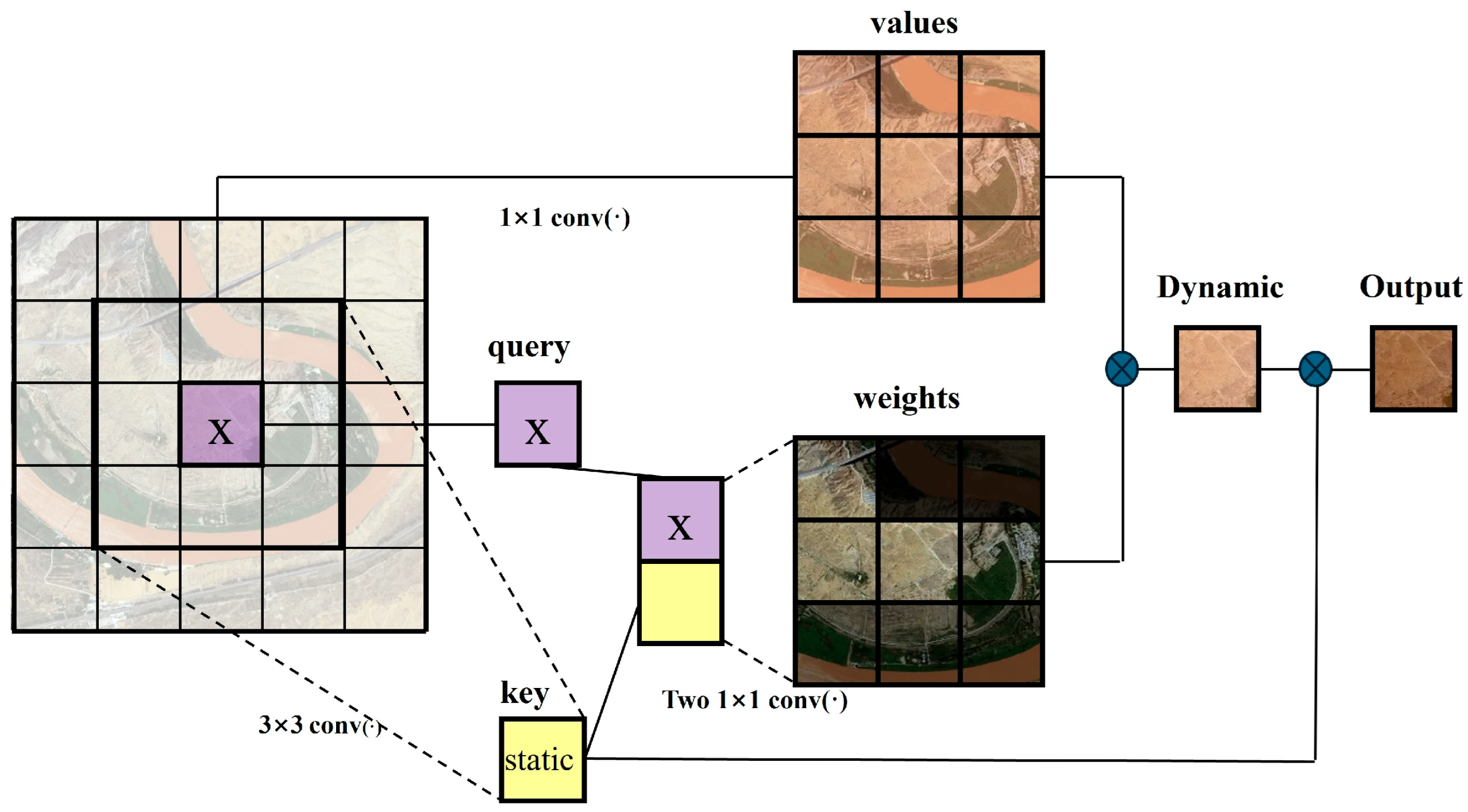
In regional groundwater change analysis, dynamics are governed by both temporal dynamics and spatial contextual dependencies from surrounding regions. To address this, a Dynamic–Static Feature Fusion (DSFF) is designed in this paper based on the COT Attention framework, integrating contextual mining and self-attention learning into a unified architecture. This approach leverages static key–value relationships while exploring dynamic feature interactions, enabling the model to capture both local temporal patterns and global spatial dependencies in time series data.

The module first extracts static contextual relationships between keys via a 3 × 3 convolution layer, followed by two successive 1 × 1 convolutional operations for self-attention computation based on queries and context keys to generate dynamic context. The static and dynamic contexts are then fused to produce the final output (Figure 6). In time series prediction tasks, the simultaneous capture of local and global sequence features is critical. As a novel attention mechanism, this module enhances the Transformer model’s feature extraction capability for time series by integrating convolutional operations with dynamic attention weight calculations.

4.

Integrated Transformer model

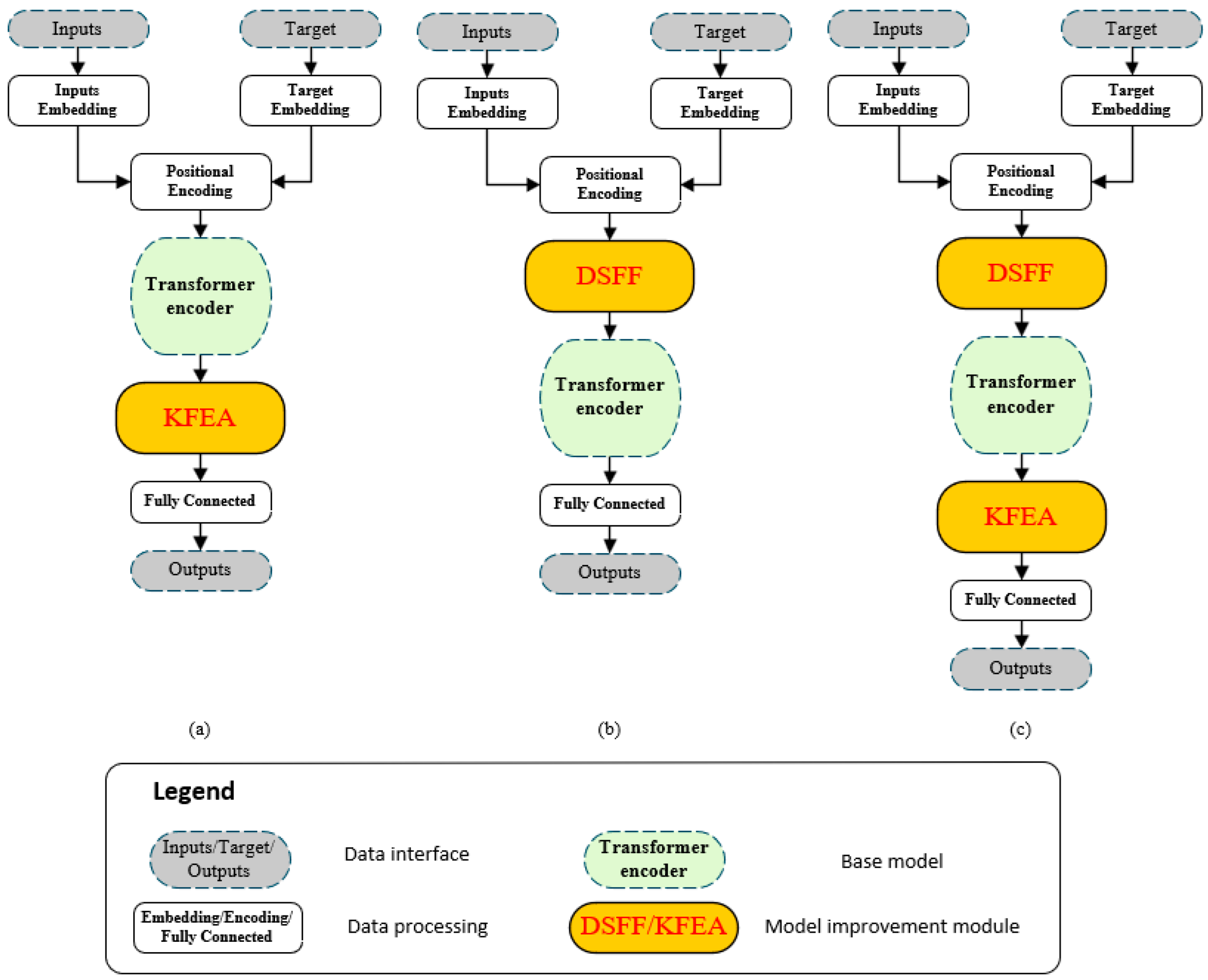
In time series tasks, SEnet exhibits specific adaptability for capturing key information in sequential data. Through its squeeze-and-excitation mechanism, SEnet effectively enhances the weights of informative features while suppressing irrelevant ones. Conversely, the COT framework’s output pattern integrating dynamic and static contexts enables comprehensive acquisition of local and global information. Therefore, in addition to independent computations using the Transformer model, this paper performs comparative analyses on combinations of DSFF, KFEA structures, and the Transformer model. The comparative analysis framework evaluates the synergistic effects of DSFF and KFEA within the Transformer architecture. The structures of the three types of variants are shown in Figure 7.

The improved models are referred to as Transformer-KFEA (a), DSFF-Transformer (b), and DSFF-Transformer-KFEA (c). In the Transformer-KFEA model, the SEnet structure is introduced at the end of the Transformer encoder, allowing the model to learn the importance weights of each channel through global average pooling and fully connected layers. This enhances the features of important channels while suppressing those of less important ones. This mechanism helps the model focus on feature dimensions with more informative content, thereby improving time series estimation accuracy. In the DSFF-Transformer model, the DSFF structure is integrated into the Transformer encoder, capturing local static context information through convolution operations and dynamically generating attention key–value pairs based on input features. This aids in better capturing both global and local information in time series estimation. The DSFF-Transformer- KFEA model combines both methods to investigate whether their combined use can jointly improve model performance.

5.

LSTM

The LSTM model, a specialized variant of recurrent neural networks (RNNs), is widely employed in sequence data analysis owing to its capability to capture long-term temporal dependencies, demonstrating notable achievements in diverse time series prediction tasks. By leveraging memory cells and gating mechanisms, LSTM exhibits significant efficacy in simulating complex temporal patterns and resolving dynamic groundwater variations over time. However, when processing extremely long sequences, LSTM may encounter challenges associated with vanishing or exploding gradient issues, which arise from the inherent limitations in propagating error signals through extended temporal steps. The gating mechanism of LSTM comprises three primary components: the forget gate, which regulates information retention; the input gate, which controls new information integration; and the output gate, which modulates state information exposure.

$${\mathrm{f}}_{\mathrm{t}}=\mathsf{\sigma }\left({\mathrm{W}}_{\mathrm{f}}\text{⋅}\right[{\mathrm{h}}_{\mathrm{t}-1},{\mathrm{x}}_{\mathrm{t}}]+{\mathrm{b}}_{\mathrm{f}})$$

(9)

$${\mathrm{i}}_{\mathrm{t}}=\mathsf{\sigma }\left({\mathrm{W}}_{\mathrm{i}}\text{⋅}\right[{\mathrm{h}}_{\mathrm{t}-1},{\mathrm{x}}_{\mathrm{t}}]+{\mathrm{b}}_{\mathrm{i}})$$

(10)

$${\mathrm{C}}_{\mathrm{t}}={\mathrm{f}}_{\mathrm{t}}\text{⊙}{\mathrm{C}}_{\mathrm{t}-1}+{\mathrm{i}}_{\mathrm{t}}\text{⊙}\tan \mathrm{h}\left({\mathrm{W}}_{\mathrm{C}}\text{⋅}\right[{\mathrm{h}}_{\mathrm{t}-1},{\mathrm{x}}_{\mathrm{t}}]+{\mathrm{b}}_{\mathrm{C}})$$

(11)

$${\mathrm{o}}_{\mathrm{t}}=\mathsf{\sigma }\left({\mathrm{W}}_{\mathrm{o}}\text{⋅}\right[{\mathrm{h}}_{\mathrm{t}-1},{\mathrm{x}}_{\mathrm{t}}]+{\mathrm{b}}_{\mathrm{o}})$$

(12)

$${\mathrm{h}}_{\mathrm{t}}={\mathrm{o}}_{\mathrm{t}}\text{⊙}\tan \mathrm{h}\left({\mathrm{C}}_{\mathrm{t}}\right)$$

(13)

In this context, $f_t$ represents the activation value of the forget gate, i_t denotes the activation value of the input gate, $C_t$ refers to the cell state, $o_t$ indicates the activation value of the output gate, and $h_t$ represents the hidden state.

As a model that also focuses on long-range dependencies and positional information, this study attempts to utilize LSTM to perform the same task and outputs the results for comparative analysis with the Transformer model and its variants.

2.3.4. Core Metrics and Hyperparameter Configuration

This study employed three core metrics—Root Mean Square Error (RMSE), Mean Absolute Error (MAE), and the Coefficient of Determination (R²). During the model training period, the information contained within each pixel was divided into an 80% training set and a 20% test set, thereby obtaining these metrics. RMSE is a metric for quantifying prediction error, calculated by averaging the squared differences between predicted and actual values, followed by taking the square root of the result. RMSE emphasizes larger prediction errors, making it more sensitive to outliers, with smaller RMSE values indicating predictions that are closer to the true values. MAE is another quantitative measure of prediction error, computed as the average of the absolute differences between predicted values and actual observations. MAE directly reflects the average magnitude of prediction errors, with smaller values indicating more accurate predictions. Unlike RMSE, MAE penalizes large errors less severely, making it more robust to outliers. R² represents the proportion of variance in the observed values that is explained by the model, with values ranging from 0 to 1. The closer R² is to 1, the higher the goodness of fit of the model.

$$\mathrm{RMSE}=\sqrt{{\displaystyle \frac{1}{\mathrm{n}}}{\sum }_{\mathrm{i}=1}^{\mathrm{n}}{({\mathrm{y}}_{\mathrm{i}}-{\widehat{\mathrm{y}}}_{\mathrm{i}})}^2}$$

(14)

$$\mathrm{MAE}={\displaystyle \frac{1}{\mathrm{n}}}{\sum }_{\mathrm{i}=1}^{\mathrm{n}}\left|y_i-{\widehat{y}}_i\right|$$

(15)

$${\mathrm{R}}^2=1-{\displaystyle \frac{{\sum }_{\mathrm{i}=1}^{\mathrm{n}}{({\mathrm{y}}_{\mathrm{i}}-{\widehat{\mathrm{y}}}_{\mathrm{i}})}^2}{{\sum }_{\mathrm{i}=1}^{\mathrm{n}}{({\mathrm{y}}_{\mathrm{i}}-\stackrel{\mathrm{-}}{\mathrm{y}})}^2}}$$

(16)

In this context, $y_i$ represents the true value of the i -the observation, ${\widehat{y}}_i$ denotes the predicted value of the i -the observation, and n refers to the number of samples.

Hyperparameter configuration (see

Table 1. Hyperparameter configuration.

Model Name	Epochs/ Patience	Learning Rate (Adam)	Dim	Self-Attention Heads	Encoder Layers	COT Convolution Kernel	SEnet Channel Compression Ratio
Transformer	200/75	0.0001	128	4	4	-	-
Transformer-KFEA	200/75	0.00005	128	4	4	-	16
DSFF-Transformer	200/75	0.0001	128	4	4	3 × 3	-
DSFF-Transformer-KFEA	200/75	0.0001	128	4	4	3 × 3	16
LSTM	200/75	0.002	-	-	-	-	-

) significantly impacts the performance and prediction accuracy of the algorithm during the model training period. For instance, insufficient iterations may lead to the results not converging to the optimal value, while excessive iterations may cause overfitting and degrade performance, thereby affecting prediction accuracy. To prevent overfitting while ensuring fitting accuracy, an early stopping mechanism is implemented in the model. Training will be terminated when the validation loss (val-loss) does not improve for a specified number of epochs, as determined by the patience parameter. By analyzing the performance of R² achieved under different iteration counts during the model training period, the training performance for each iteration configuration was determined. Consequently, the maximum number of iterations was set to 200, with a patience value of 75. Other hyperparameters were determined in a similar manner. Potential effective hyperparameter options were identified by preliminary experimental results and reviewing relevant studies [41,42]. For the Transformer and its variants, potential optimal selections were obtained for parameters such as learning rate, dimension, self-attention heads, and encoder layers, and the optimal combination with the highest R² was determined through grid search testing on the test set (A partial illustration of the Transformer model prototype is shown in

Table 2. Results of hyperparameter optimization via grid search (evaluated by test set R²).

Model Name	Epochs/ Patience	Learning Rate (Adam)	Dim	Self-Attention Heads	Encoder Layers	Test Set R2
Transformer	200/75	0.0001	32	4	4	0.59
Transformer	200/75	0.00005	32	4	4	0.52
Transformer	200/75	0.00001	32	4	4	0.5
Transformer	200/75	0.0001	64	4	4	0.62
Transformer	200/75	0.00005	64	4	4	0.54
Transformer	200/75	0.00001	64	4	4	0.53
Transformer	200/75	0.0001	128	4	4	0.68
…	…	…	…	…	…	…

). For model variants incorporating the DSFF module, with other parameters fixed, combinations of COT Convolution Kernel sizes of 3 × 3 and 5 × 5 were tested, respectively. The 5 × 5 kernel showed significantly poorer R² performance than the 3 × 3 kernel across almost all pixels in the test set. For model variants incorporating the KFEA module, the SENet Channel Compression Ratio was tested in a similar manner, with 16 being selected as it yielded the best R² performance among the tested values of 8, 16, and 32. The specific hyperparameter configurations are as follows.

3. Results

3.1. Comparison of Estimation Performance of Various Machine Learning Models

This study employed various machine learning models to estimate groundwater levels in the Yellow River Basin. During the model training period, well groundwater level data were converted into areal datasets using inverse distance weighting (IDW) and Kriging interpolation methods. These datasets were then resampled to match 0.25° × 0.25° resolution remote sensing pixels, thereby obtaining paired data of well groundwater levels and remote sensing-derived groundwater storage. Subsequently, time series estimations were performed for groundwater levels across all 1277 pixels.

3.1.1. Influence of Spatial Interpolation Method on Model Estimation

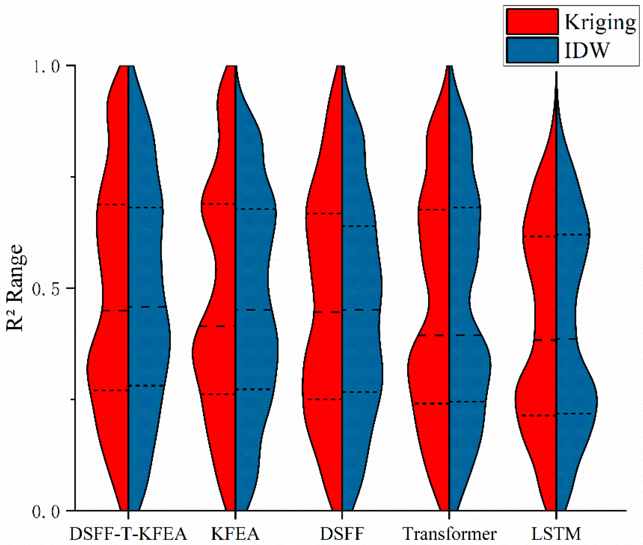
The two interpolation schemes exhibit differential impacts on the model architectures: negligible influence on the baseline LSTM and Transformer models, moderate effect on the KFEA-integrated variant, and more pronounced impact on the DSFF module-incorporated architecture. Under the IDW scheme, the DSFF-Transformer model demonstrates a 10.7% reduction in R² variance compared to the baseline Transformer, whereas the DSFF-Transformer-KFEA model shows only a 0.5% variance decrease.

This phenomenon can be attributed to the DSFF model’s reliance on surrounding data for static information acquisition, where different interpolation schemes cause variations in peripheral data to exert influence. The DSFF model’s behavior of collecting relatively large-scale data and employing time series estimation introduces additional information into the estimation process. This approach helps reduce sensitivity to outliers but may simultaneously introduce new noise. Consequently, the number of samples decreases in high and low R² zones while increasing in intermediate R² zones, as shown in Figure 8.

The RMSE values for the five models under the dual interpolation scheme across the entire region are 0.292, 0.299, 0.311, 0.317, and 0.331, respectively, with corresponding MAE values of 0.227, 0.227, 0.241, 0.240, and 0.250 (

Table 3. R², RMSE, and MAE of each model.

Index	Interpolation Scheme	DSFF-Transformer-KFEA	Transformer-KFEA	DSFF- Transformer	Transformer	LSTM
R2	Kriging	0.478	0.468	0.461	0.450	0.404
	IDW	0.476	0.464	0.451	0.453	0.408
RMSE	Kriging	0.467	0.479	0.494	0.494	0.534
	IDW	0.759	0.778	0.805	0.811	0.865
MAE	Kriging	0.362	0.369	0.376	0.380	0.408
	IDW	0.589	0.596	0.617	0.620	0.658

). The results show that Kriging method yields lower error metrics compared to the IDW method. The IDW method assigns weights solely based on distance, which may lead to the “bull’s-eye effect” where excessive weight is placed on nearby data points, causing concentric variations in the interpolation surface. In regions with uneven distribution of monitoring points (such as dense urban areas) or spatial correlation features (such as directionality or anisotropy), the distance-based weight distribution of IDW may result in non-uniform interpolation outcomes.

3.1.2. Influence of Machine Learning Model on Estimation

Significant differences in predictive performance exist across the 1277 sample regions for the same model structure, with the percentage of samples for which the models fail to produce valid predictions (R² < 0) shown in the table. The results indicate that the use of different spatial interpolation schemes has a certain impact on data availability.

Under the Transformer model’s core architecture, the IDW method yields fewer unusable points. Among the model variants, the Transformer-KFEA demonstrates the highest data adaptability, with the lowest percentages of unusable points under both spatial interpolation schemes (5.40% and 5.87%, respectively). In contrast, the DSFF-Transformer model exhibits the lowest data adaptability (12.37% and 11.12%), as shown in

Table 4. Proportion of invalid samples (R² < 0) in each model.

Model	DSFF-Transformer-KFEA	Transformer-KFEA	DSFF-Transformer	Transformer	LSTM
Kriging	9.08%	5.40%	12.37%	8.61%	9.40%
IDW	8.07%	5.87%	11.12%	8.93%	10.18%

, a phenomenon likely attributed to the DSFF module’s reliance on structured data inputs during the 3 × 3 convolution step. This dependency may limit its predictive efficacy in regions with pronounced anomalies, as the module requires coherent spatial context for optimal feature extraction. The KFEA module’s channel-wise weighting mechanism appears to mitigate sensitivity to data irregularities, contributing to the Transformer-KFEA model’s enhanced robustness across interpolation schemes.

After excluding samples with ineffective predictions, Figure 8 (the dashed line represents the quartiles and median) presents the distribution of R² values for samples obtained using different machine learning models through five sets of paired violin plots, where each pixel is treated as a sample. Within each set, the left violin plot corresponds to Kriging interpolation results, while the right represents IDW results. The R² values of the five models primarily cluster within the range of 0.3 to 0.7, illustrating that time series forecasting models are substantially influenced by the volatility of real-world data. In regions with distinct data characteristics, the models effectively capture trend patterns, whereas in areas with obscure data features or anomalous fluctuations (such as extreme hydrological events), the models’ learning capacity is notably compromised, leading to a sharp decline in R² values. This results in a distribution roughly resembling a “dumbbell” shape.

After excluding a small subset of non-representative samples, the table presents the R², RMSE, and MAE metrics for the five models under two spatial interpolation schemes. The average RMSE values across the entire region for the dual interpolation scheme are 0.613, 0.629, 0.650, 0.653, and 0.699 for the five models, with corresponding MAE values of 0.476, 0.483, 0.497, 0.500, and 0.533. The results demonstrate that the Transformer model exhibits reduced prediction volatility and higher accuracy compared to the LSTM model.

Since our model primarily improves upon existing frameworks, the traditional Diebold–Mariano (DM) test tends to be conservative—often failing to reject the null hypothesis that new and old models exhibit no significant difference. Therefore, this study employs the Clark–West (CW) test for significance testing, a method designed for comparing nested models. In CW tests of the enhanced models, the DSFF-Transformer-KFEA demonstrated statistically significant improvements over both the Transformer prototype and LSTM model in approximately 56.2% and 57.4% of the 1277 pixel-based samples, respectively.

Furthermore, the accuracy improvement conferred by the DSFF module is found to be limited, potentially due to the module introducing additional information that propagates the influence of short-term significant fluctuations in local data caused by extreme hydrological events in the original dataset. In contrast, the KFEA structure effectively filters the new information introduced by the DSFF module, assigning preferential weights to informative channels. As a result, the model integrating both KFEA and DSFF modules demonstrates a notable accuracy enhancement relative to the baseline model and single-module configurations. These findings highlight the synergistic effect of channel-wise feature weighting (via KFEA) and contextual–temporal attention (via DSFF) in mitigating interpolation-induced noise and improving predictive robustness.

The regional average of the deviation from long-term mean groundwater level between model estimates and well groundwater level across the Yellow River Basin is visualized in Figure 9, demonstrating the propagation of model estimates from more recent years toward older years, depicting the prediction performance across the entire study area. The correlation coefficients between the estimated groundwater levels obtained by the Transformer model and its variants and the actual well groundwater level from ground-based wells are 0.829, 0.822, 0.847, and 0.838, respectively. During periods of relatively stable hydrological changes, all models effectively capture and fit the trends of groundwater variations. Analysis of well measured data and GRACE-derived signals indicates that the models can accurately resolve annual periodic fluctuations and long-term trends in groundwater storage.

Notably, the Transformer model exhibits certain limitations in learning local extrema, leading to systematic overestimation of low values and underestimation of high values. Among the model variants, the Transformer-KFEA demonstrates superior trend simulation, achieving the highest correlation coefficient. This performance advantage is likely related to the KFEA module’s capability to prioritize critical components in long-term time series information, enabling enhanced trend fitting across the Yellow River Basin. The module’s channel-wise weighting mechanism may enhance the model’s sensitivity to dominant hydrological signals, thereby mitigating the impact of noise in extreme value regions.

3.2. Spatial Representation of Estimation Results

The R² values of the five models across the upper, middle, and lower reaches of the Yellow River are tabulated (

Table 5. Models R² for different basins.

Basin	Interpolation Scheme	DSFF-Transformer -KFEA	Transformer -KFEA	DSFF- Transformer	Transformer	LSTM
Upstream	Kriging	0.446	0.430	0.425	0.441	0.387
	IDW	0.496	0.445	0.471	0.489	0.405
midstream	Kriging	0.495	0.498	0.490	0.435	0.413
	IDW	0.445	0.461	0.419	0.410	0.396
downstream	Kriging	0.880	0.875	0.783	0.796	0.637
	IDW	0.785	0.777	0.800	0.804	0.650

). Under Kriging interpolation, the average R² values for the five models in the upper, middle, and lower reaches are 0.426, 0.466, and 0.793, respectively, whereas IDW yields corresponding values of 0.461, 0.426, and 0.763. Both interpolation methods show the highest estimation accuracy in the lower reach, primarily due to the significantly higher density of monitoring wells in this region. This dense monitoring network enables comprehensive spatial coverage of groundwater conditions. Conversely, the upper reach exhibits lower accuracy owing to sparse well distribution and extremely limited monitoring points.

Notably, Kriging outperforms IDW in the relatively data-rich middle reach, while IDW demonstrates slightly better performance in the data-sparse upper reach. This discrepancy may be linked to Kriging’s underlying assumptions of stationarity and isotropy, which are more susceptible to violation in areas with sparse sampling. In contrast, IDW’s simpler distance-based weighting mechanism does not rely on such strict statistical assumptions, potentially conferring greater robustness in regions with limited well observational data.

The results demonstrate that the DSFF module’s incorporation of peripheral data provides fundamental support for upstream areas lacking well-measured data. Simultaneously, in the middle reaches affected by soil erosion, broader data collection mitigates adverse impacts from systematic anomalies in gravity satellite observations. However, introducing additional data may propagate deficiencies from other regions to adjacent pixels. Consequently, standalone application of the DSFF module yields limited accuracy improvements. After implementing the KFEA module’s screening mechanism—which filters incorporated data—this limitation is effectively overcome. The integrated dual-module model consequently achieves the highest accuracy in both data-sparse upstream regions and data-deficient middle reach areas.

The overall performance of different models in the Yellow River Basin is visualized in Figure 10, showing that the high and low accuracy areas of each model exhibit similar spatial distributions: lower accuracy in the central and western regions, and higher accuracy in the northeastern regions. This pattern is likely associated with the fact that a significant portion of the central and western regions are in mountainous areas and the Loess Plateau, which are characterized by complex geological structures, substantial fluctuations in surface water flow, and the impact of soil erosion. The heterogeneous geological structures in these regions may diminish the representativeness of monitoring points in reflecting the actual groundwater conditions of their surrounding areas. Long-term soil erosion can also lead to surface mass migration, thereby affecting the gravity readings of GRACE satellites and indirectly impacting on estimation accuracy. The accuracy in the source region of the Yellow River is also relatively limited. While geological structural changes in this area may exert some influence on gravity satellite readings, the associated mass variations are not significant when compared to the systematic mass transfer from soil erosion in the middle reaches of the Yellow River. Therefore, the primary cause of the poorer accuracy performance in the source region does not lie in this factor, but rather in the lower density of monitoring wells, as shown in Figure 1.

In the eastern part of the Yellow River (i.e., the middle and lower reaches), regions with intensive human activities typically feature a denser network of monitoring wells, which enhances the ability of monitoring point data to reflect the groundwater conditions of adjacent areas, contributing to improved estimation accuracy in these regions. The results highlight the combined influence of geological heterogeneity and anthropogenic factors on the spatial distribution of model performance in hydrological estimation.

The spatial distribution of high and low accuracy regions under data distribution constraints exhibits similar patterns across all models, though the proportions of regions with R² > 0.7 differ significantly: 30.2%, 25.8%, 30.0%, 26.2%, and 19.5% for the five models, respectively. The DSFF-Transformer-KFEA and DSFF-Transformer models show the highest proportions of high-value regions, while the LSTM model exhibits the lowest. This indicates that the DSFF module’s capability to capture both dynamic and static features enhances the Transformer model’s regional estimation stability, effectively expanding the area with relatively higher accuracy. In contrast, the LSTM model lacks such a mechanism, leading to more limited estimation accuracy.

Notably, the Transformer-KFEA model displays a lower proportion of high-value regions than the baseline Transformer model, suggesting that applying squeeze-and-excitation operations to sequence features may, in certain contexts, impact the model’s fitting performance. The results highlight the trade-off between channel-wise feature weighting (via KFEA) and contextual feature integration (via DSFF) in modulating spatial prediction accuracy, underscoring the importance of architectural design in aligning with data distribution characteristics.

The annual groundwater level change rates derived from different estimation models are −2.65, −2.15, −2.19, −1.90, and −2.26 mm/month, exhibiting a consistent west-high, east-low spatial distribution trend, as show in Figure 11. The western basin shows relatively minor groundwater level declines, whereas several northeastern areas exhibit more pronounced groundwater level declines. This pattern is primarily attributed to the western region serving as the Yellow River’s headwater area, characterized by sparse population density and limited anthropogenic water consumption. Additionally, upstream glacial meltwater has increased slightly due to global warming, contributing to groundwater recharge. In contrast, the northeastern basin—marked by higher population density and flat topography—experiences intensive groundwater extraction for agricultural and industrial activities, leading to sustained declines in groundwater levels.

Subplot (f) of Figure 11 displays the average change rate of remote sensing-derived groundwater storage over the 20-year period. This reflects groundwater trends obtained solely from remote sensing data, exhibiting a general pattern of higher values in the west and lower values in the east. This spatial distribution remains broadly consistent with results derived from machine learning models incorporating well groundwater data. Comparison with the other five that while remote sensing data alone can provide an approximate understanding of regional groundwater changes during the study period, they fail to reflect differences in groundwater level responses when identical storage changes occur at different locations. Concurrently, Transformer models and their variants not only consider current monthly groundwater storage changes but also incorporate historical information and spatial context. This approach facilitates more accurate conversion of groundwater storage data into groundwater level estimates without requiring high-precision specific yield information across the entire region.

4. Discussion

In this study, four Transformer model variants and an LSTM model were employed for groundwater level estimation. Experimental results indicate that the Transformer model integrating a dynamic-static fusion perception mechanism and KFEA outperforms the traditional LSTM model, with R² improvements ranging from 16.7% to 18.3%. This performance advantage stems from the model’s ability to mitigate critical limitations of conventional time series estimation methods in groundwater prediction: unclear long-term dependency modeling, insufficient spatiotemporal information integration, and suboptimal key feature weighting.

4.1. Application of Self-Attention Mechanism in Estimation

The Transformer model, by virtue of its unique self-attention mechanism, enables direct modeling of temporal dependencies over arbitrary distances. Through this global dependency modeling framework, it significantly mitigates the issue of ambiguous long-term dependencies in traditional LSTM/GRU models, which arises from gradient vanishing in long time series sequences. This advantage is corroborated by numerous studies. For instance, Azad Deihim [43] applied the Transformer encoder to capture latent spatiotemporal dependencies in multivariate time series for Beijing PM2.5 prediction and metro interstate traffic volume forecasting, demonstrating a 20.6% reduction in RMSE compared to LSTM, which aligns with our findings. Siying Zhu [44] leveraged the Transformer’s attention mechanism to resolve long-term trends in meteorological datasets, incorporating a time series clustering framework for unsupervised learning. In meteorological applications, this approach yielded a 13.6% reduction in MAE relative to DLinear, further validating the Transformer’s superiority in capturing temporal dynamics. These results highlight the potential of Transformer models in resolving long-term temporal variations in groundwater levels, offering promising prospects for enhancing estimation accuracy and interpretability in hydrological modeling.

4.2. Application of Spatial Information

By integrating the DSFF module into the Transformer framework, this study presents a hybrid modeling approach that aligns closely with hydrological realities for groundwater level estimation while preserving the model’s inherent characteristics. This is achieved through the introduction of a DSFF mechanism and a combined “spatial convolution + temporal attention” design, which significantly mitigates the issue of insufficient spatiotemporal information integration. These findings are corroborated by complementary research efforts. For instance, Lingtong Min [45] demonstrated in remote sensing small target detection that mixed modeling of spatial context and temporal channel information substantially reduces the likelihood of valuable information being obfuscated or overlooked. By introducing COT into the decoupling head, their model achieved a 0.4% increase in mAP@0.5:0.95. Similarly, Deli Zhu [46] employed a DSFF module in post-fire forest restoration studies to enhance the model’s capacity for exploring spatial context in complex environments, resulting in a 3.26% improvement in mean intersection over union (mIoU) relative to ResNet. These results highlight that groundwater level prediction requires the consideration of both temporal features within pixels and spatial features between pixels. The introduction of the DSFF module effectively expands feature acquisition pathways, which is conducive to improving the accuracy of large-scale groundwater temporal estimation using remote sensing data. This approach underscores the importance of integrating contextual–temporal attention mechanisms in hydrological modeling to better resolve the spatiotemporal complexity of groundwater systems.

4.3. Application of Feature Filtering

The Transformer variant with the KFEA, by introducing a channel feature adaptive weighting mechanism while preserving the original model characteristics, coupled with a compression–excitation operation after the encoder output, is capable of automatically assigning weights to different channel features. This improves the issue of inaccurate key element weight allocation. Numerous research findings support this perspective. Chen Liu’s research [47] in the domain of multi-dimensional time series classification, extracted features across the time, variance, and channel dimensions of multi-dimensional time series data, guiding the features into the channel interactions within a squeeze-and-excitation network. This successfully enhanced the model’s representation ability. Compared to the baseline model ResNet, the model achieved a 3.31% improvement in weighted average accuracy, further validating our viewpoint.

4.4. Application of Improved Model

The dual-module coupling model integrates the two modules, fully leveraging the advantages of both. The DSFF module introduces additional information at the encoder’s front end, while the KFEA processes this information via adaptive weighting at the encoder output stage. This design ensures a reasonable weight distribution between the introduced static information and the dynamic information captured by the Transformer model through the temporal attention mechanism. Experimental results show that the coupled model achieves an R² improvement of approximately 5.1% to 6.2% compared to the Transformer prototype.

This analysis reveals that prior studies utilizing GRACE terrestrial water storage for groundwater estimation predominantly focused on temporal sequence variations at specific locations, with limited consideration of multi-source information weighting and long-term temporal dependencies. Our findings indicate that incorporating surrounding contextual information, rationally assigning channel weights to input data, and accounting for long-term correlations during single-pixel estimation processes can facilitate a clearer and more accurate characterization of long-term groundwater variation patterns. This approach addresses the limitations of conventional methods by integrating spatial contextual cues and temporal dependency modeling, thereby enhancing the interpretability of groundwater dynamics at both local and regional scales.

4.5. Deficiencies and Prospects

In the upper reaches of the Yellow River, sparse well observational data points hinder robust estimation, while in the middle reaches’ loss plateau region, long-term soil–water erosion impacts GRACE-derived gravity measurements. This study demonstrates that integrating surrounding pixel information during groundwater estimation alleviates these effects. However, systematic supplementation of in situ observations and quantification of erosion-induced mass transfer lie beyond the current scope but represent promising directions for future research.

5. Conclusions

This study investigates groundwater level time series estimation in the Yellow River Basin using five deep learning algorithms: Transformer, Transformer-KFEA, DSFF-Transformer, DSFF-Transformer-KFEA, and LSTM. The key conclusions are as follows: (1) The Transformer-based estimation model effectively captures long-range temporal dependencies in groundwater time series, demonstrating significantly higher accuracy than the LSTM model. (2) The dynamic–static fusion perception mechanism and KFEA address critical limitations of conventional estimation methods, including neglect of spatial contextual information and ambiguous feature weighting. These innovations enhance estimation accuracy without substantial increases in computational complexity. (3) IDW exhibits poorer performance than Kriging in regions with sparse data, indicating that distance-based interpolation schemes lack flexibility for low-quality datasets. (4) Groundwater levels in the Yellow River Basin show a fluctuating downward trend during our research period (2003–2024), which downward trend increases from upstream to downstream. The self-attention estimation model proposed herein demonstrates potential for application in other basins. It is noted that this research focuses on satellite pixel-scale analysis (0.25° × 0.25°), where topographic, geomorphic, and geological heterogeneities within pixels may compromise estimation precision. Future studies will investigate finer-resolution groundwater distributions and incorporate additional hydrological parameters to enhance model fidelity.

References

1. van der Gun, J. Groundwater and Global Change; United Nations Educational, Scientific and Cultural Organization (UNESCO): Paris, France, 2012; pp. 1–42+44. [Google Scholar]
2. Siebert, S.; Burke, J.; Faures, J.M.; Frenken, K.; Hoogeveen, J.; Döll, P.; Portmann, F.T. Groundwater use for irrigation—A global inventory. Hydrol. Earth Syst. Sci. 2010, 14, 1863–1880. [Google Scholar] [CrossRef]
3. Vorosmarty, C.J.; Green, P.; Salisbury, J.E.; Lammers, R.B. Global Water Resources:Vulnerability from Climate Change and Population Growth. Science 2000, 289, 284–288. [Google Scholar] [CrossRef]
4. Jasechko, S.; Perrone, D. Global groundwater wells at risk of running dry. Science 2021, 372, 418–421. [Google Scholar] [CrossRef]
5. Shin, Y.S. On the “Groundwater”. Logging Landslides 1976, 13, 16–21. [Google Scholar] [CrossRef]
6. Ding, K.; Zhao, X.; Cheng, J.; Yu, Y.; Couchot, J.; Zheng, K.; Lin, Y.; Wang, Y. GRACE/ML-based analysis of the spatiotemporal variations of groundwater storage in Africa. J. Hydrol. 2025, 647, 132336. [Google Scholar] [CrossRef]
7. Peng, M.; Lu, Z.; Zhao, C.; Motagh, M.; Bai, L.; Conway, B.D.; Chen, H. Mapping land subsidence and aquifer system properties of the Willcox Basin, Arizona, from InSAR observations and independent component analysis. Remote Sens. Environ. 2022, 271, 112894. [Google Scholar] [CrossRef]
8. Ma, R.; Chen, K.; Andrews, C.B. Methods for Quantifying Interactions Between Groundwater and Surface Water. Annu. Rev. Environ. Resour. 2024, 49, 623–653. [Google Scholar] [CrossRef]
9. Noorduijn, S.L.; Harrington, G.A.; Cook, P.G. The representative stream length for estimating surface water–groundwater exchange using Darcy’s Law. J. Hydrol. 2014, 513, 353–361. [Google Scholar] [CrossRef]
10. Thanh, N.N.; Thunyawatcharakul, P.; Ngu, N.H.; Chotpantarat, S. Global review of groundwater potential models in the last decade: Parameters, model techniques, and validation. J. Hydrol. 2022, 614, 128501. [Google Scholar] [CrossRef]
11. Yang, M.; Liu, H.; Meng, W. An analytical solution of the tide-induced groundwater table overheight under a three-dimensional kinematic boundary condition. J. Hydrol. 2021, 595, 125986. [Google Scholar] [CrossRef]
12. Islam, Z.; Abdel-Aty, M.; Mahmoud, N. Using CNN-LSTM to predict signal phasing and timing aided by High-Resolution detector data. Transp. Res. Part C Emerg. Technol. 2022, 141, 103742. [Google Scholar] [CrossRef]
13. Alabdulkreem, E.; Alruwais, N.; Mahgoub, H.; Dutta, A.K.; Khalid, M.; Marzouk, R.; Motwakel, A.; Drar, S. Sustainable groundwater management using stacked LSTM with deep neural network. Urban Clim. 2023, 49, 101469. [Google Scholar] [CrossRef]
14. Turkoglu, M.O.; Stefano, A.; Wegner, J.D.; Schindler, K. Gating Revisited: Deep Multi-layer RNNs That Can Be Trained. IEEE Trans. Pattern Anal. Mach. Intell. 2021, 44, 4081–4092. [Google Scholar] [CrossRef]
15. Choudhary, A.; Arora, A. Assessment of bidirectional transformer encoder model and attention based bidirectional LSTM language models for fake news detection. J. Retail. Consum. Serv. 2024, 76, 103545. [Google Scholar] [CrossRef]
16. Zhang, H.; Shafiq, M.O. Survey of transformers and towards ensemble learning using transformers for natural language processing. J. Big Data 2024, 11, 25. [Google Scholar] [CrossRef]
17. Su, L.; Zuo, X.; Li, R.; Wang, X.; Zhao, H.; Huang, B. A systematic review for transformer-based long-term series forecasting. Artif. Intell. Rev. 2025, 58, 80. [Google Scholar] [CrossRef]
18. Subhadarsini, S.; Kumar, D.N.; Govindaraju, R.S. Enhancing Hydro-climatic and land parameter forecasting using Transformer networks. J. Hydrol. 2025, 655, 132906. [Google Scholar] [CrossRef]
19. Xiong, Z.; Zhang, Z.; Gui, H. A Meteorology-Driven Transformer Network to Predict Soil Moisture for Agriculture Drought Forecasting. IEEE Trans. Geosci. Remote Sens. 2025, 63, 4405818. [Google Scholar] [CrossRef]
20. Zhang, D.; Madsen, H.; Ridler, M.E.; Kidmose, J.; Jensen, K.H.; Refsgaard, J.C. Multivariate hydrological data assimilation of soil moisture and groundwaterhead. Hydrol. Earth Syst. Sci. 2016, 20, 4341–4357. [Google Scholar] [CrossRef]
21. Boo, K.B.W.; El-Shafie, A.; Othman, F.; Khan, M.H.; Birima, A.H.; Ahmed, A.N. Groundwater level forecasting with machine learning models: A review. Water Res. 2024, 252, 121249. [Google Scholar] [CrossRef]
22. Kostić, S.; Stojković, M.; Guranov, I.; Vasović, N. Revealing the background of groundwater level dynamics: Contributing factors, complex modeling and engineering applications. Chaos Solitons Fractals 2019, 127, 408–421. [Google Scholar] [CrossRef]
23. Sabzehee, F.; Amiri-Simkooei, A.; Iran-Pour, S.; Vishwakarma, B.; Kerachian, R. Enhancing spatial resolution of GRACE-derived groundwater storage anomalies in Urmia catchment using machine learning downscaling methods. J. Environ. Manag. 2023, 330, 117180. [Google Scholar] [CrossRef]
24. Wang, Y.; Sun, L.; Li, H. Monthly 8-km Gridded Meteorological Dataset for the Upper and Middle Reaches of the Yellow River Basin (1980–2015). J. Glob. Change Data Discov. 2022, 6, 25–36, 184–195. [Google Scholar]
25. Akl, M.; Thomas, B.F. Challenges in applying water budget framework for estimating groundwater storage changes from GRACE observations. J. Hydrol. 2024, 639, 131600. [Google Scholar] [CrossRef]
26. Shi, Z.; Zhu, X.; Tang, Y. Analysis of Terrestrial Water Storage Changes and Influencing Factors in China Based on GRACE Satellite Data. Arid. Land Geogr. 2023, 46, 1397–1406. [Google Scholar]
27. Castellazzi, P.; Ransley, T.; McPherson, A.; Slatter, E.; Frost, A.; Shokri, A.; Wallace, L.; Crosbie, R.; Janardhanan, S.; Kilgour, P.; et al. Assessing Groundwater Storage Change in the Great Artesian Basin Using GRACE and Groundwater Budgets. Water Resour. Res. 2024, 60, e2024WR037334. [Google Scholar] [CrossRef]
28. Zhang, L.; Ke, P.; Zhang, L. Study on Spatiotemporal Variation of Groundwater Storage in China Based on GRACE Data. J. Hydroecol. Ecol. 2024, 9–17. [Google Scholar]
29. Gong, H.; Pan, Y.; Zheng, L.; Li, X.; Zhu, L.; Zhang, C.; Huang, Z.; Li, Z.; Wang, H.; Zhou, C. Long-term groundwater storage changes and land subsidence development in the North China Plain (1971–2015). Hydrogeol. J. 2018, 26, 1417–1427. [Google Scholar] [CrossRef]
30. Castellazzi, P.; Martel, R.; Rivera, A.; Huang, J.; Pavlic, G.; Calderhead, A.I.; Chaussard, E.; Garfias, J.; Salas, J. Groundwater depletion in Central Mexico: Use of GRACE and InSAR to support water resources management. Water Resour. Res. 2016, 52, 5985–6003. [Google Scholar] [CrossRef]
31. Diego-Alejandro, S.-A.; Alexandra, S.; Luiz-Carlos, F. Characterization of groundwater storage changes in the Amazon River Basin based on downscaling of GRACE/GRACE-FO data with machine learning models. Sci. Total Environ. 2024, 912, 168958. [Google Scholar]
32. Hellwig, J.; de Graaf, I.E.M.; Weiler, M.; Stahl, K. Large-scale assessment of delayed groundwater responses to drought. Water Resour. Res. 2020, 56, e2019WR025441. [Google Scholar] [CrossRef]
33. Lu, F.; You, W.; Fan, D. Inversion of Water Storage and Ocean Mass Changes in Mainland China over the Last Decade from GRACE RL05 Data. Acta Geod. Cartogr. Sin. 2015, 44, 160–167. [Google Scholar]
34. Frappart, F.; Ramillien, G. Monitoring Groundwater Storage Changes Using the Gravity Recovery and Climate Experiment (GRACE) Satellite Mission: A Review. Remote Sens. 2018, 10, 829. [Google Scholar] [CrossRef]
35. Chen, J.L.; Wilson, C.R.; Tapley, B.D.; Yang, Z.L.; Niu, G.Y. 2005 drought event in the Amazon River basin as measured by GRACE and estimated by climate models. J. Geophys. Res. 2009, 114, B05404. [Google Scholar] [CrossRef]
36. Long, D.; Yang, W.; Sun, Z. Satellite Gravimetry Inversion and Basin Water Balance for Groundwater Storage Changes in the Haihe Plain. J. Hydraul. Eng. 2023, 54, 255–267. [Google Scholar]
37. Kang, X.; Li, L.; Sun, C. Sustainability Study of Groundwater in the Gansu Section of the Yellow River Basin Based on GRACE and GLDAS Data. J. Desert Res. 2024, 44, 196–206. [Google Scholar]
38. UNESCO. The United Nations World Water Development Report 2022: Groundwater: Making the Invisible Visible. 2022. Available online: https://www.unwater.org/publications/un-world-water-development-report-2022 (accessed on 24 July 2024).
39. Cao, J.; Xiao, Y.; Long, D. Monitoring Groundwater Storage Changes in the North China Plain by Combining Satellite Gravimetry and Well Data. Geomat. Inf. Sci. Wuhan Univ. 2024, 5, 805–818. [Google Scholar]
40. Zhu, X.-H.; Li, K.-R.; Deng, Y.-J.; Long, C.-F.; Wang, W.-Y.; Tan, S.-Q. Center-Highlighted Multiscale CNN for Classifcation of Hyperspectral Images. Remote Sens. 2024, 16, 4055. [Google Scholar] [CrossRef]
41. Huang, J.; Yan, H.; Chen, Q.; Liu, Y. Multi-Granularity Temporal Embedding Transformer Network for Traffc Flow Forecasting. Sensors 2024, 24, 8106. [Google Scholar] [CrossRef]
42. Vasan, V.; Sridharan, N.V.; Vaithiyanathan, S.; Aghaei, M. Detection and classification of surface de-fects on hot-rolled steel using vision transformers. Heliyon 2024, 10, e38498. [Google Scholar] [CrossRef]
43. Deihim, A.; Alonso, E.; Apostolopoulou, D. STTRE: A Spatio-Temporal Transformer with Relative Embeddings for multivariate time series forecasting. Neural Netw. 2023, 168, 549–559. [Google Scholar] [CrossRef] [PubMed]
44. Wang, Y.; Wu, X.; Zhang, J.; Wang, W.; Zheng, L.; Shang, J. Series clustering and dynamic periodic patching-based transformer for multivariate time series forecasting. Appl. Soft Comput. 2025, 174, 112980. [Google Scholar] [CrossRef]
45. Min, L.; Fan, Z.; Lv, Q.; Reda, M.; Shen, L.; Wang, B. YOLO-DCTI: Small Object Detection in Remote Sensing Base on Contextual Transformer Enhancement. Remote Sens. 2023, 15, 3970. [Google Scholar] [CrossRef]
46. Zhu, D.; Yang, P. Study on the Evolutionary Characteristics of Post-Fire Forest Recovery Using Unmanned Aerial Vehicle Imagery and Deep Learning: A Case Study of Jinyun Mountain in Chongqing, China. Sustainability 2024, 16, 9717. [Google Scholar] [CrossRef]
47. Liu, C.; Wei, Z.; Zhou, L.; Shao, Y. Multidimensional time series classification with multiple attention mechanism. Complex Intell. Syst. 2025, 11, 14. [Google Scholar] [CrossRef]
Figure 1. Distribution of groundwater monitoring wells in the Yellow River Basin.
Water 17 02318 g001
Figure 2. Time series prediction Transformer model structure.
Water 17 02318 g002
Figure 3. Multi-head attention parallel layers.
Water 17 02318 g003
Figure 4. (a) Self-attention estimation, (b) tend to learn recent months, (c) tend to learn similar months (schematic only), and (d) tend to learn from near to far.
Water 17 02318 g004
Figure 5. Distribution of attention scores at different layers.
Water 17 02318 g005
Figure 6. Schematic diagram of COTAttention.
Water 17 02318 g006
Figure 7. Transformer model variants: (a) Transformer-KFEA (b) DSFF-Transformer (c) DSFF-Transformer-KFEA.
Water 17 02318 g007
Figure 8. R2 distribution of each model.
Water 17 02318 g008
Figure 9. Comparison between the well groundwater level and models.
Water 17 02318 g009
Figure 10. R2 distribution under Kriging method.
Water 17 02318 g010
Figure 11. (ae) Groundwater level change rate under different models (f) Remote sensing of groundwater storage change rate.
Water 17 02318 g011