Article

Comparative Assessment Using Different Topographic Change Detection Algorithms for Gravity Erosion Quantification Based on Multi-Source Remote Sensing Data

College of Geomatics, Xi’an University of Science and Technology, Xi’an 710054, China
*
Author to whom correspondence should be addressed.
Water 2025, 17(15), 2309; https://doi.org/10.3390/w17152309
Submission received: 2 July 2025 / Revised: 29 July 2025 / Accepted: 1 August 2025 / Published: 3 August 2025
(This article belongs to the Special Issue Applications of Remote Sensing and GISs in River Basin Ecosystems)

Abstract

Gravity erosion is one of the main physical processes of soil erosion and sediment sources in catchments, and its spatiotemporal patterns and driving mechanisms are seriously understudied, mainly due to the the great difficulties in monitoring and quantifying. This study obtained gravity erosion amounts by runoff scouring experiments on the field slope of the hilly–gully region of the Chinese Loess Plateau. The terrain point cloud before and after gravity erosion was obtained based on the TLS, SfM and the fusion of single-scan TLS and SfM, and then the gravity erosion was estimated by four terrain change detection algorithms (DoD, C2C, C2M and M3C2). Results showed that the M3C2 algorithm plus fused data had the highest quantization accuracy among all the algorithms and data sources, with a relative error of 14.71%. The fused data combined with M3C2 algorithm performed much better than other algorithms and data sources for the different gravity erosion magnitudes (mean relative error < 17.00%). The DoD algorithm plus TLS data were preferable for collapse areas, while the M3C2 algorithm plus TLS was suitable for the alcove area. This study provides a useful reference for the monitor and quantitative research of gravity erosion in complex topographic areas.

1. Introduction

Gravity erosion (e.g., landslide, rockfall, avalanche and debris flow) refers to the processes in which rock and soil masses lose balance and move under the influence of gravity [1,2]. Gravity erosion is widely distributed globally [3,4,5,6], and its frequency and scale may sharply increase under the background of global climate change [7]. However, gravity erosion is difficult to monitor due to the fact that it mostly occurs in steep slope areas with complex terrain, leading to the research on its precise quantification and driving mechanism still being in its infancy [8,9]. Therefore, it is crucial to investigate the accuracy and applicability of different monitoring technologies and detecting algorithms.
The monitoring technologies for gravity erosion include traditional technologies and remote sensing technologies. Traditional monitoring technologies mainly include isotope tracers [10,11,12], tape measurement [13,14,15], field investigations [16,17,18] and erosion pins [19,20,21]. However, although the above-mentioned method can obtain the temporal changes in gravity erosion in the slope–gully system to a certain extent, it lacks detailed spatial distribution information of gravity erosion and erosion morphological characteristics [8,22]. Furthermore, traditional monitoring methods such as the erosion pins require manual measurement, which may introduce relatively large human deviations [23]. Therefore, to gain a deeper understanding of gravity erosion types, occurrence processes and mechanisms, more refined research on gravity erosion is needed. With the wide application of modern high-precision monitoring technologies (e.g., three-dimensional laser scanning and close-range photogrammetry) in the field of erosion, the study of gravity erosion has gradually entered the stage of precise measurement and visualization [24,25,26]. Close-range photogrammetry is a passive remote sensing technology. It can instantly obtain a large amount of geometric and physical information of the measured area by producing rather dense point clouds, which can be employed to extract high-precision surface morphology information [27]. This method has the advantages of high accuracy and low cost [28]. However, it easily influenced by the external environment (such as ambient light conditions, wind, etc.) during data acquisition and unable to penetrate the vegetation [29]. The 3D laser scanner is an active remote sensing technology which is not affected by visible light and is capable of penetrating vegetation partly [30,31]. This technology can obtain high-resolution point cloud data of the underlying surface quickly and accurately [32,33]. In addition, the fusion of laser scanning data and photogrammetry data has also been applied to topographic change monitoring, especially for the complex terrain area [33,34]. Then, based on the high-precision point cloud data, the terrain characteristics and erosion amount can be achieved by constructing the high-precision DEM or comparing the point cloud before and after erosion. Thus, the 3D laser scanner, photogrammetry and the corresponding fused data can provide effective approaches for the quantitative research of gravity erosion [18,35,36].
The topographic change detection algorithms are the key to the terrain change detection and subsequent gravity erosion quantification [37]. Several common terrain change detection algorithms mainly include the cloud-to-cloud comparison with closest point technique (C2C) [38], cloud-to-mesh distance or cloud-to-model distance (C2M) [39], DEM of difference (DoD) [40], and multiple model-to-model cloud comparison (M3C2) [41]. The C2C algorithm is conducted by quantifying the distances between points in the reference point cloud and the comparison point cloud, while the C2M algorithm calculates the distances between the meshes generated by the reference point cloud and points from the comparison point cloud. The calculation processes of the two algorithms take a relatively short time, and are typically used to quickly identify the location and extent of terrain changes. The M3C2 algorithm measures the difference in terrain changes by using the orthogonal distance between the reference point cloud and the comparison point cloud [42]. The DoD algorithm is one of the most commonly used algorithms for large-scale terrain change monitoring [43]. This algorithm constructs a DEM using multiple terrain point cloud datasets and quantifies terrain changes through DEM differences. Previous studies have compared qualitatively the accuracy of these algorithms on topographic and volumetric changes in channel sedimentation based on 3D laser scanning [44,45]. However, the quantification accuracy and applicability of different algorithms for small-scale gravity erosion monitoring in complex terrain areas has been rarely assessed [46].
Gravity erosion is one of the dominant soil erosion processes in the hilly–gully loess plateau. The occurrence processes of gravity erosion are of a stochastic nature, which makes field observation difficult. Field experiments (e.g., rainfall or scouring simulations) of a natural slope–gully system are able to replicate the terrain development characteristic and gravity erosion processes, and thus facilitate an effective monitoring and quantification. Therefore, the scouring experiment was conducted in a typical catchment of the hilly–gully loess plateau (i.e, Xindiangou catchment) to simulate the topographic features of gravity erosion occurring. Three data sources (TLS, SfM and fused data) and four algorithms (C2C, C2M, DoD and M3C2) were used to quantify the gravity erosion amount. Based on this, we aimed to (1) quantify the gravity erosion using different data sources and various change detection algorithms at the slope scale, and (2) assess the accuracy of the combination of different data sources and change detection on gravity erosion qualification under different magnitudes and geomorphic units.

2. Materials and Methods

2.1. Study Site

The study area is located in the Xindiangou watershed, Suide County, Yulin City, Shaanxi Province, China. The geographical coordinates of the watershed are 110°16′45″ E to 110°20′00″ E and 37°29′00″ N to 37°31′00″ N (Figure 1a). The region is characterized by a northwest–southeast orientation and a typical loess gully landform. With a watershed area of 1.44 km2, it is a representative exemplar of the hilly–gully region of the loess plateau. The elevation of the study area ranges from 820 to 1010 m, with a significant relative relief of up to 190 m. The mean annual temperature is approximately 10.20 °C, and the mean annual precipitation is 476 mm [5]. The precipitation is unevenly distributed, with over 60% concentrated between June and September [47]. The predominant soil type in the watershed is Calcaric Regosol (commonly referred to as loess-like soil or huangmian-tu), which is characterized by its deep profile, loose texture, and low resistance to erosion. These soil properties contribute to severe gravity erosion and soil and water loss. Consequently, the region exhibits a high gully density, deeply incised valleys, steep gully slopes, and intense headward erosion at the gully heads.

2.2. Design of Experimental Runoff Plots

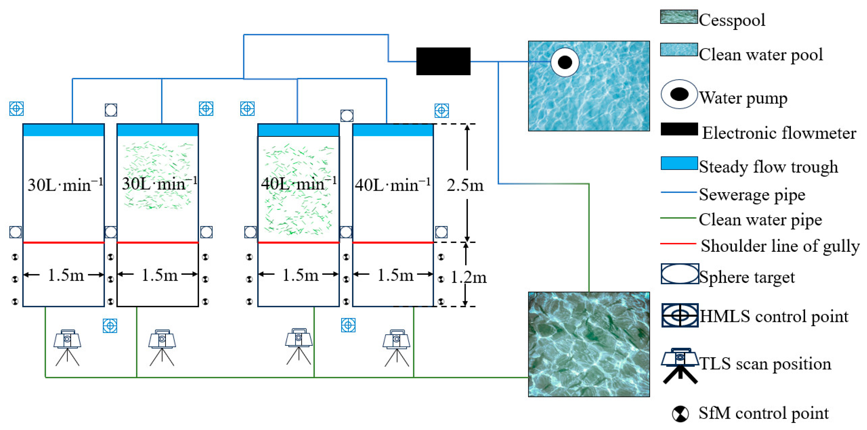
The experimental area consisted of four runoff plots, a clean water reservoir, and a wastewater collection tank. The clean water reservoir was connected to a headbox at the top of the slope via flexible pipes. An electromagnetic flowmeter was integrated into the system to precisely control the flow rate, thereby providing a stable water supply to the experimental slopes to simulate natural rainfall or runoff conditions. Each experimental plot comprised a hill slope section measuring 2.5 m in length and 1.5 m in width, and a gully slope measuring 1.2 m in height and 1.5 m in width. The original topographic characteristics of the inter-gully slope were preserved, with a gradient of 20° (±3°). The plots were bordered on both sides by iron sheets, which protruded 0.1 m above the ground surface (Figure 1d). The gully wall within each plot was manually excavated to form a vertical face of 90° (±3°).
To ensure a controlled and stable inflow, a headbox was installed at the top of the slope. A flexible pipe connected the clean water reservoir to the headbox, and the flow rate was regulated by an electromagnetic flowmeter to meet the stringent hydraulic requirements of the experiment. The four experimental plots were designated as Plot A, Plot B, Plot C and Plot D (Figure 1c). To simulate different ground cover conditions, vegetation was removed from Plots A and D. In contrast, vegetation was retained in Plots B and C to serve as a comparative basis for studying the effects of vegetation on flow dynamics (Figure 2). In this study, different flow rates and slope characteristics (vegetation or non-vegetation plot) were designed in our experiment plots. This is primarily intended to simulate different initial morphology where gravitational erosion occurred under various natural conditions.

2.3. Experimental Procedure

Prior to the formal simulated gravity erosion experiment, the terrain of the runoff plot was first flushed with water to bring it to a critical state for gravity erosion. Based on local rainfall conditions and the morphology of the hill slope within the runoff plot, flow rates were confirmed for the flushing process based on formulaic calculations as follows.
F = W D I A cos θ
where F is the discharge flow rate (L/min), W is the width of the experimental plot (m), D is the width of the upstream (m), I is the rainfall intensity (mm/min), A is the upstream area (m2), θ is the gradient of the hillslope (°), is the run-off coefficient. Considering the specifics of the experiment, W , D , I , A were set as 1.5 m, 5 m, 0.3–1.2 mm/min, 300–400 m2, θ was set 16°, was set 0.32–0.57. According to the results of the calculations, the input flow rates for Plot A and Plot C were set to 40 L/min, which represented the surface runoff rate under large rainfall conditions. The input flow rates for Plot B and Plot D were set to 30 L/min, which represented the surface runoff rate under conventional rainfall conditions (Figure 2).
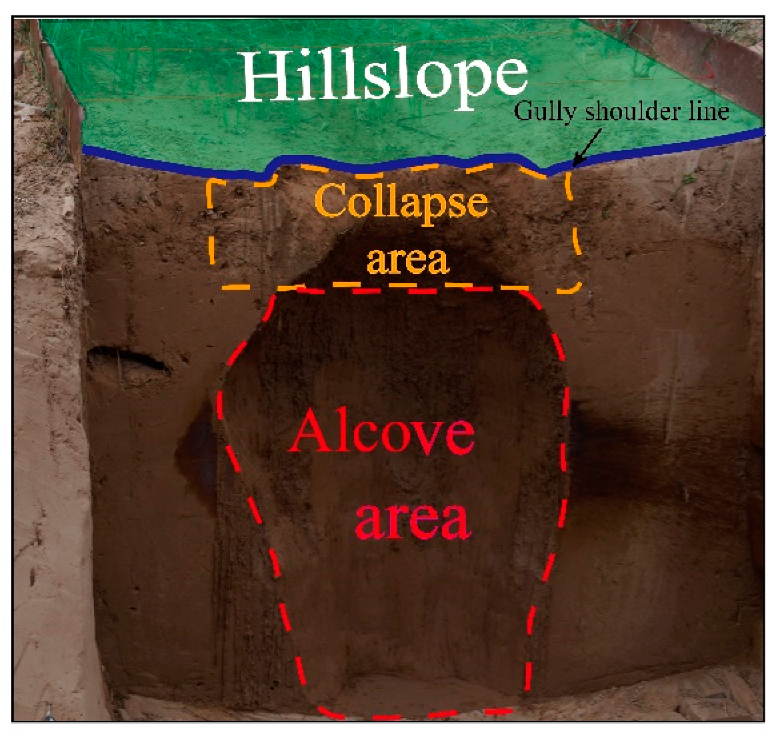
The resulting topography after scouring experiment was shown in Figure 3. The upper part of the gully slope was found to be susceptible to mass movement, which primarily manifested as collapse; this area was subsequently defined as the collapse area. Meanwhile, the lower part of the gully slope was often undercut by hydraulic erosion, leading to the formation of an inward-hollowed cavity. This region was defined as the alcove area (Figure 3).
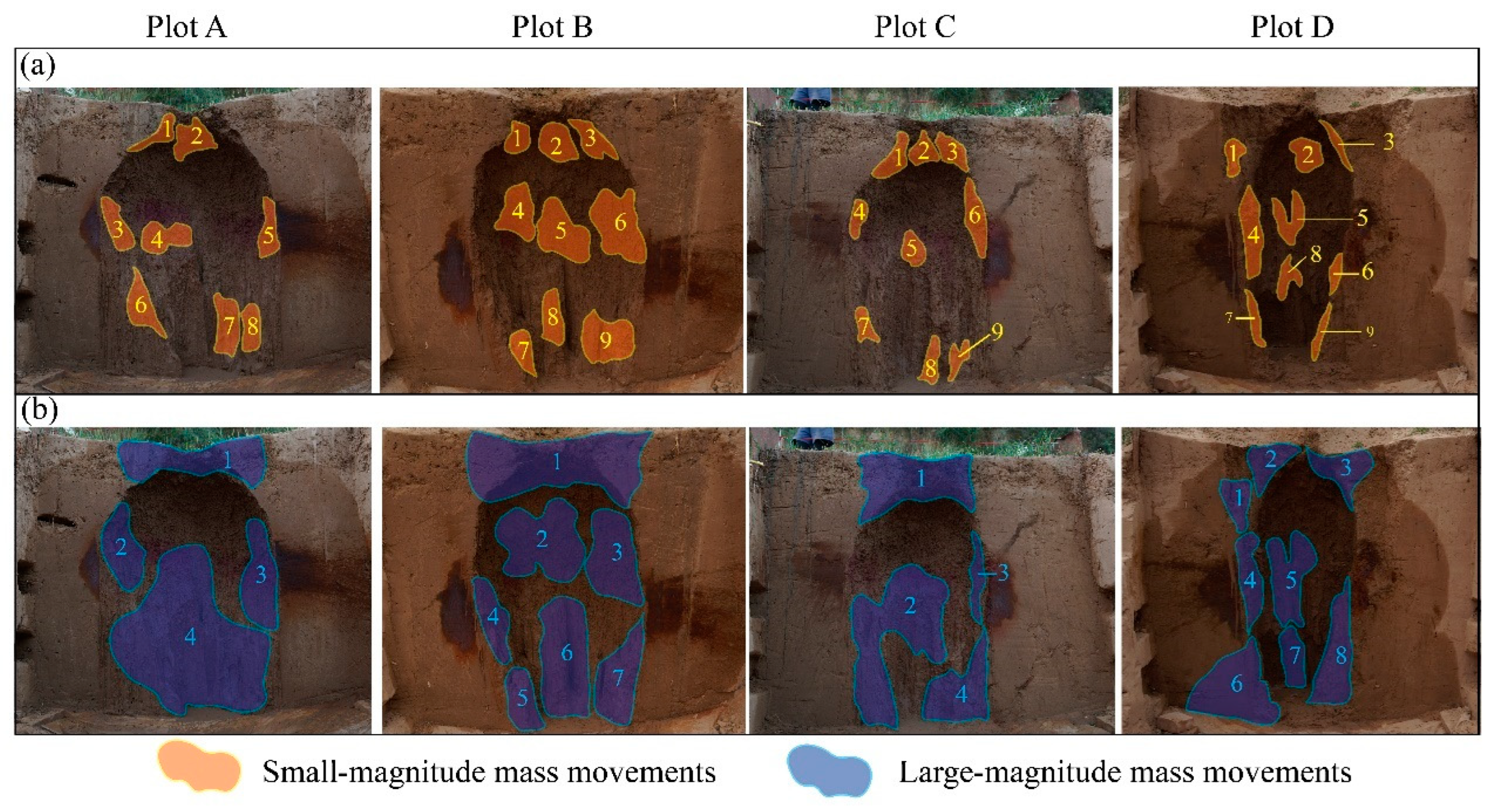
After the terrain was flushed to a suitable state, the runoff plot was left to stand for 24 h to ensure a relatively uniform soil moisture content throughout the plot. Subsequently, a number of gravity erosion samples were collected from the areas on the gully slope identified as susceptible to gravity erosion. Each sample was carefully and completely collected into a sample bag. The simulated gravity erosion experiment involved sample collection in two batches. The first batch of samples was intended to simulate small-magnitude gravity erosion events, with each sample volume controlled to be under 500 cm3. The second batch aimed to simulate large-magnitude events, with sample volumes ranging from 500 cm3 to 9000 cm3. In total, this experiment collected 35 small-magnitude gravity erosion samples and 23 large-magnitude gravity erosion samples (Figure 4).

2.4. Point Cloud Data Acquisition and Processing

2.4.1. Point Cloud Data Acquisition

Four sets of stone piers were installed in the upper, lower, left and right positions of two adjacent runoff plots, respectively, to serve as mounts for the target spheres (Figure 2). The terrestrial laser scanning (Leica ScanStation C10, Leica Geosystems, Heerbrugg, Switzerland) was used in this study to acquire the three-dimensional terrain point cloud. It operates with a green laser at a wavelength of 532 nm, achieving a point spacing of less than 1 mm at a scanning range of up to 50 m. The scanner has a vertical and horizontal field of view of 270° and 360°, respectively, resulting in a blind spot within a 45° cone directly beneath the instrument’s nadir. To avoid occlusion between the target spheres during the scanning process, the four stone piers were set up to be non-coplanar. Furthermore, care was taken to ensure that the 3D laser scanner was not positioned to be collinear with any two target spheres. To capture the 3D terrain point cloud data as completely as possible, the scanner’s station positions were strategically placed at various angles relative to the gully slope during the scanning process. Typically, the number of scan positions was 4 to 6. The scanning range was defined as the area between 0.5 m and 2 m from the gully slope. The scanning angle was between 80° and 120°.
Structure from Motion (SfM) was employed to reconstruct a high-resolution 3D model of the gully slope topography using high-definition imagery acquired with a digital camera (Sony ILCE7RM3 camera, Sony Corporation, Tokyo, Japan). To mitigate potential anomalies in the reconstructed 3D terrain data due to topographic shadows, SfM data acquisition was conducted between 2 PM and 6 PM. During the photography process, it was crucial to ensure that the ground control points (GCPs) were clearly visible in the images, maintaining an image overlap of at least 80%. Photography was carried out following a defined flight path or shooting trajectory. The gully slope terrain photographs were taken to include as many GCPs as possible. For areas with topographic occlusions, additional supplementary photographs were taken as needed.

2.4.2. Point Cloud Data Processing

The raw point cloud data must undergo processes such as stitching, registration and filtering to obtain a complete topographic dataset of the gully slope. The data processing workflow primarily includes the following steps. Based on the Leica Cyclone software version 7.4.1 (https://leica-geosystems.com/products/laser-scanners/software/leica-cyclone/leica-cyclone-register-360 (accessed on 2 August 2025)), the raw point clouds from individual stations were registered with each other by referencing the target spheres that were in place during the scanning process. Then the spatial alignment was performed between different scan sets (i.e., data from different experimental sessions) using the target spheres as a common reference in the CloudCompare software version 2.1 (https://www.danielgm.net/cc/ (accessed on 2 August 2025)). This step ensures that all point cloud data of the gully slope topography reside within a single, unified coordinate system. Finally, using TerraSolid version 08.11.09.292 (https://terrasolid.com/software-downloads/ (accessed on 2 August 2025)), noise points and non-ground points (e.g., vegetation) within the gully slope data were manually removed from the point cloud.
The processing of the SfM point cloud data involved the following steps. Any blurry photographs were manually identified and removed from the dataset. The feature points were detected and matched across the images using ContextCapture software Version 4.4.10 (https://www.bentley.com/software/itwin-capture-modeler/ (accessed on 2 August 2025)). Subsequently, the position and orientation (pose) of the camera for each photograph were calculated. The 3D coordinates of the ground control points (GCPs), derived from the TLS point cloud data, were used as a reference. These GCP coordinates were then imported and assigned to their corresponding locations in the photographs to perform a georeferenced 3D reconstruction. The generated point cloud was then processed using TerraSolid tools, where noise points and non-ground points (e.g., vegetation) on the gully slope were manually removed.
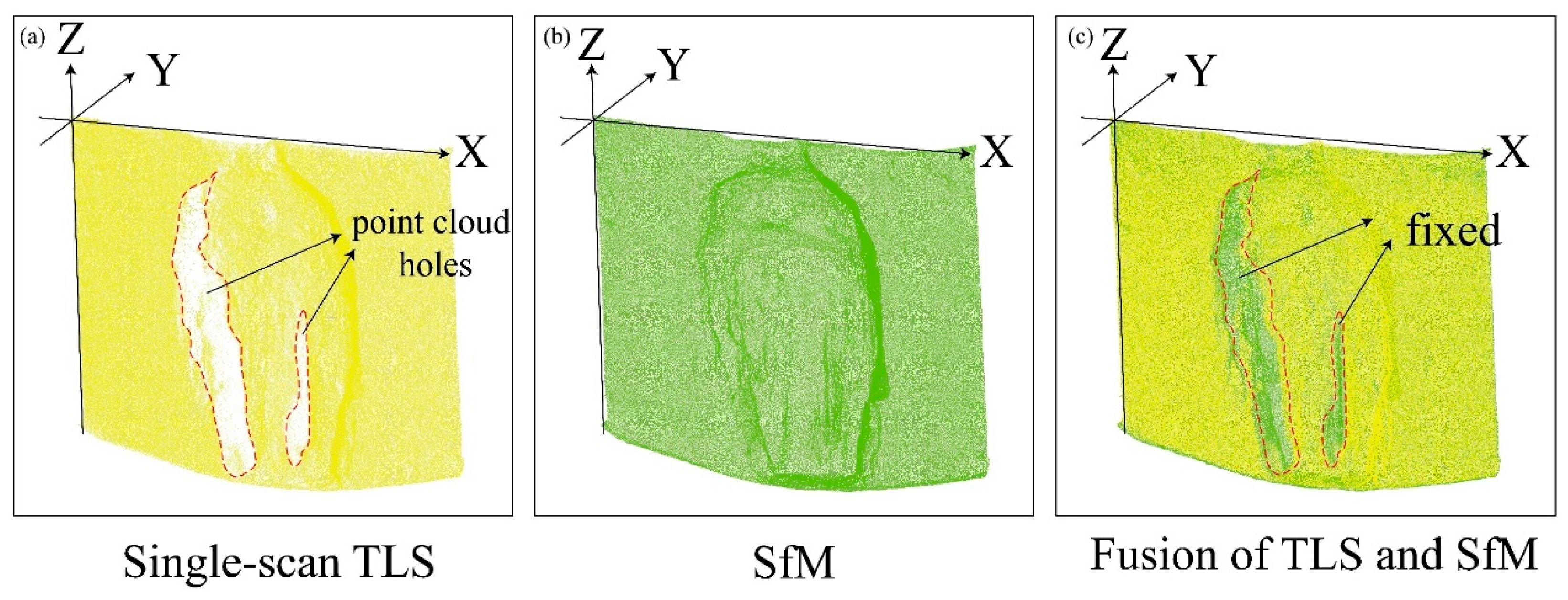
The TLS point cloud data from the station positioned directly facing the gully slope was used as the reference baseline (Figure 2) for fusion with the SfM data. This fusion process primarily involved two steps: coarse registration and fine registration. The TLS point cloud from a single station and the SfM point cloud had already been approximately aligned into the same coordinate system, completing the coarse registration step. At this stage, the two datasets were roughly overlapping. For the fine registration between them, the Iterative Closest Point (ICP) algorithm was employed [48]. The examples of a single-source point cloud and a fused point cloud appeared as shown in Figure 5.

2.5. Data Processing

2.5.1. Sample-Based Gravity Erosion Quantization

At the conclusion of the entire experiment, the soil bulk density was measured at the upper, middle and lower sections of the gully slope in each runoff plot using the cutting ring method. The formula is as follows:
ρ = M i V
where ρ is the soil bulk density (g·cm−3), M i is the mass of the soil sample (g), V is the volume of the ring cutter (cm3). The actual volume of each gravity erosion sample was calculated by dividing the sample’s mass by the soil bulk density of its corresponding location.

2.5.2. Gravity Erosion Quantization Based on Point Cloud Data

The volume of gravity erosion was calculated by applying four different change detection methods—Cloud-to-Cloud (C2C), Cloud-to-Mesh (C2M), DEM of Difference (DoD), and Multiscale Model-to-Model Cloud Comparison (M3C2)—to the TLS, SfM, and fused single-station TLS and SfM datasets, respectively.
(1)
C2C Algorithm:
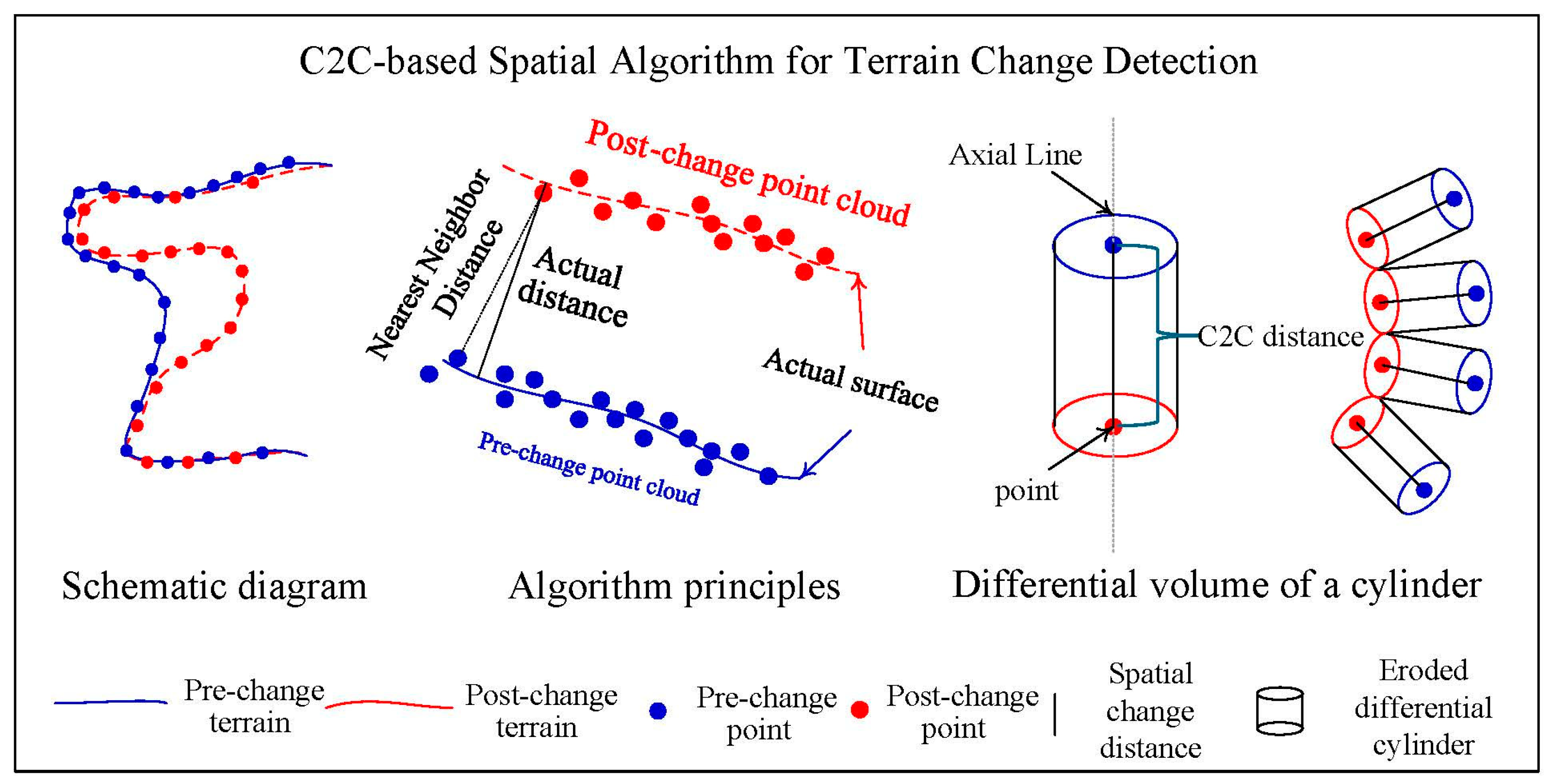
The Cloud-to-Cloud (C2C) algorithm enables rapid calculation of distances between point clouds by directly comparing two point cloud datasets, allowing for a fast and straightforward analysis [49,50]. It employs nearest neighbor search methods, such as the Hausdorff distance and k-d trees, to find the closest point in the reference point cloud for each point in the compared cloud (Figure 6). The core concept is to discretize the volume of change between the reference and compared point clouds into numerous small cylinders, with each cylinder containing only a single point from the target cloud. The C2C distance for a target point, which is an unsigned value (i.e., absolute distance), is defined as the height of its corresponding cylinder. The base area of this cylinder is defined as the reciprocal of the local point cloud surface density. The final formula for the volume of change is then derived from Equation (3):
V = Σ i = 1 n s i × D C 2 C i
where i is the index of a given point in the point cloud, s i is the reciprocal of the surface density at the i-th point, D C 2 C i is the C2C distance at that point.
(2)
C2M Algorithm:
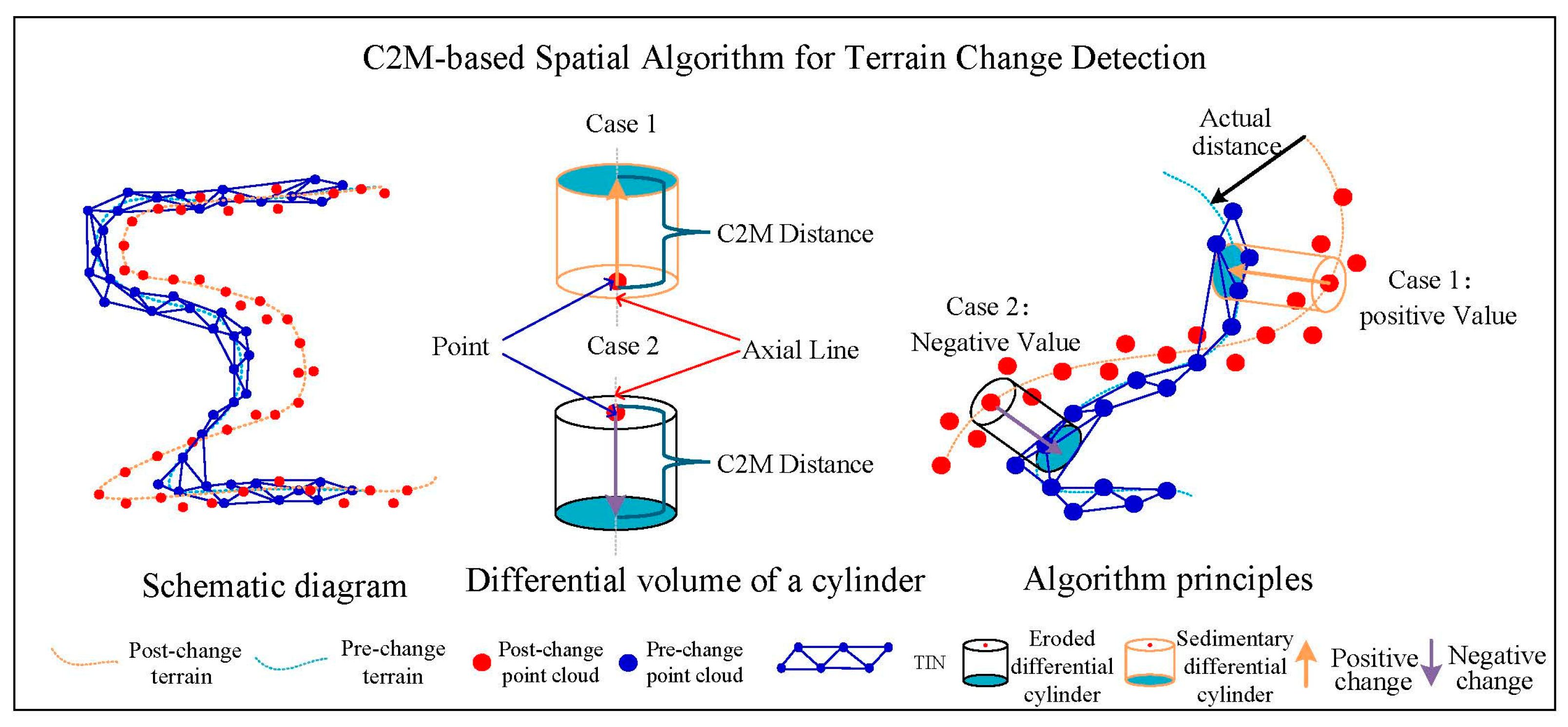
The Cloud-to-Mesh (C2M) algorithm is currently one of the most commonly used algorithms for topographic change detection [51]. Unlike the C2C algorithm, C2M calculates the spatial distance by comparing each point in a point cloud to the nearest triangle in a reference mesh/model (Figure 7). The distance between the point cloud and the mesh is derived from Equation (4):
d = A i x i + B i y i + C i z i + D i A i 2 + B i 2 + C i 2 ¯
where (xi, yi, zi) are the coordinates of an arbitrary point p in the point cloud, A i x i + B i y i + C i z i + D i = 0 is the plane equation of the nearest mesh triangle to that point. Erosion and deposition are then calculated according to Equation (3).
(3)
DoD Algorithm
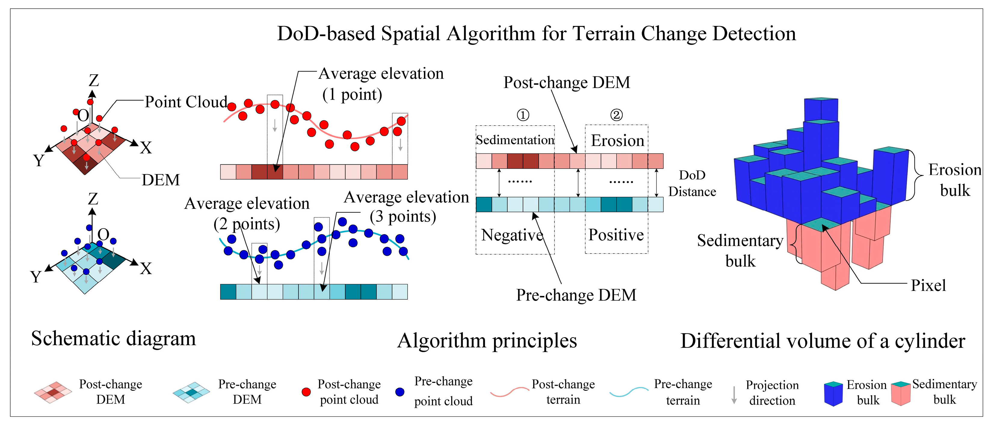
The DEM of Difference (DoD) algorithm was first applied to the field of topographic change detection by Lane et al. [52]. Its core principle involves interpolating the reference and target point clouds into separate DEMs and then calculating the difference between the two DEMs on a cell-by-cell basis (Figure 8). The volume of change is derived from Equation (5):
V = Δ z i × S C e l l × d i r
where V is volume of change (cm3), Δ z i is the vertical distance of the i-th pixel (cm), S C e l l is the area of a single grid cell (cm2), d i r is the direction of change, numerically equal to ±1.
In this study, prior to the computation of the DEM of Difference (DoD), all point clouds corresponding to gravitational erosion features were rotated to an optimal orientation. Specifically, the point clouds representing features in the central portion of the gully slope were rotated about the x-axis, whereas those on the lateral slopes of the gully were rotated about the y-axis. This procedure ensures the vertical alignment of the post-event terrain point cloud directly above the pre-event terrain point cloud. Furthermore, a grid size of 0.005 m was utilized for the analysis.
(4)
M3C2 Algorithm
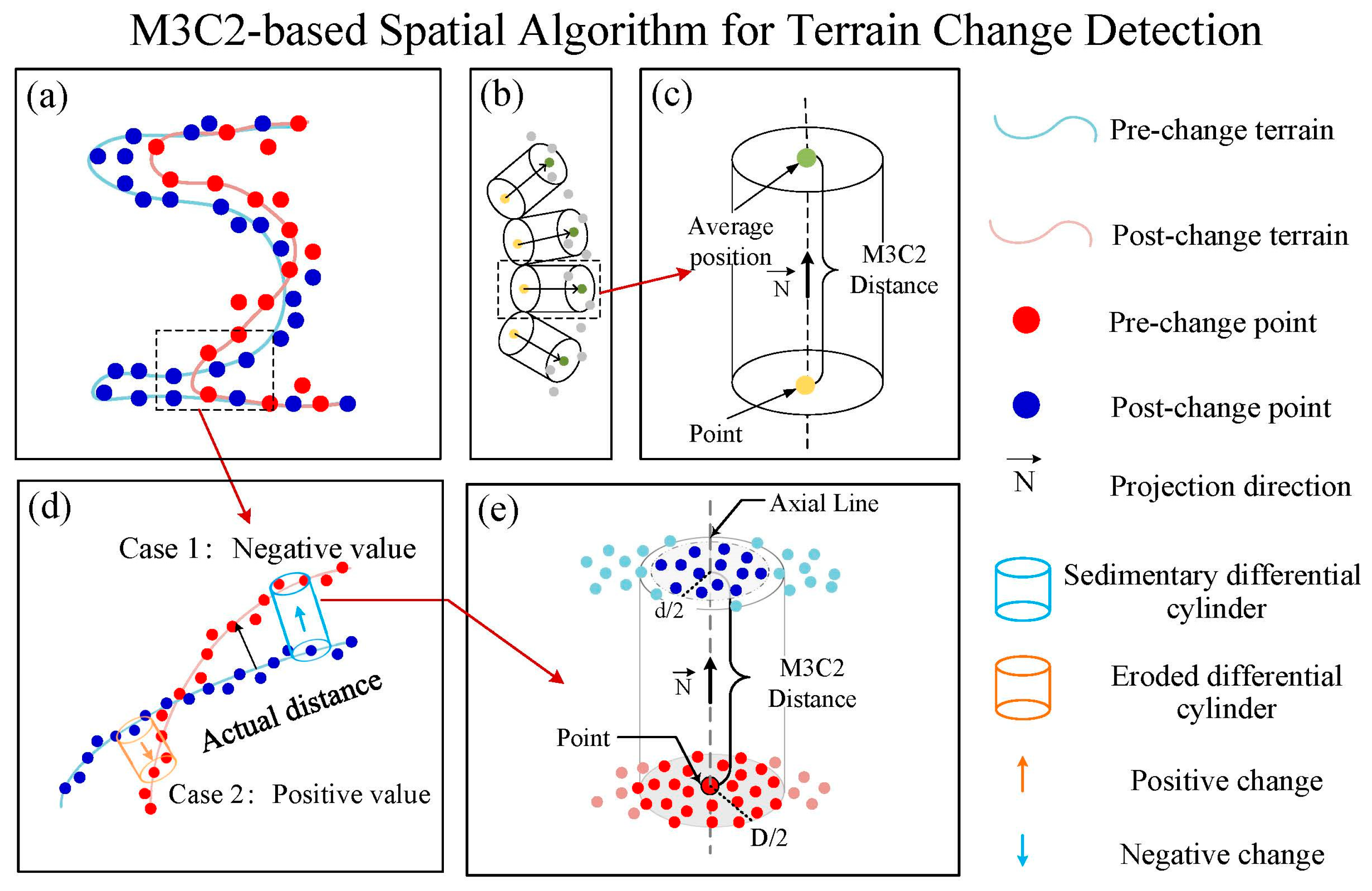
The Multiscale Model-to-Model Cloud Comparison (M3C2) algorithm, proposed by Lague [42], is a robust algorithm based on direct point cloud comparison. The algorithm incorporates two key parameters: D (normal scale) and d (projection scale). The algorithm first fits a plane to the neighborhood of each point i in the reference point cloud, defined by a radius of D/2. The normal vector of this plane is then calculated. Subsequently, a cylinder with a radius of d/2 is created, oriented along the direction of this normal vector and passing through the point i. This defined cylinder intersects with both point clouds, generating two subsets of points, n1 and n2. Each subset is then projected onto the cylinder’s axis, resulting in two distance distributions. The mean value of each distribution is calculated to determine the average positions of the point clouds along the normal vector, denoted as i1 and i2. The distance between i1 and i2 along this axis is then considered the topographic change at that point (Figure 9). Furthermore, in the M3C2 method, the level of detection (LoD) was used to distinguish the true (significant) topographic changes based on registration errors and local roughness. After removing the LoD from the distance between i1 and i2, the M3C2 distance could be obtained to calculate the corresponding erosion and deposition by Equation (3).

2.5.3. Accuracy Assessment

The absolute error (AE) and relative error (RE) were used to assess the quantification accuracy of different algorithms, which were calculated as follows:
A E = x μ
R E = x μ μ
where x is the volume of change quantified by the different topographic change detection algorithms, μ is the true value of the volume of change.
In this study, the indicators of underestimation (UE) rate, overestimation (OE) ratio and consistent estimation (CE) ratio were used to assess the quantization accuracy of different algorithms for each single sample based on the relative error. Specifically, the samples with relative error lower than −5% were defined as underestimated. Conversely, samples with relative error higher than +5% were defined as overestimated. The samples with relative error ranging from −5% to +5% were considered as consistent estimation t, indicating a relatively small deviation from the true value.

3. Results

3.1. Spatial Differences of Various Algorithms in Topographic Change Quantification

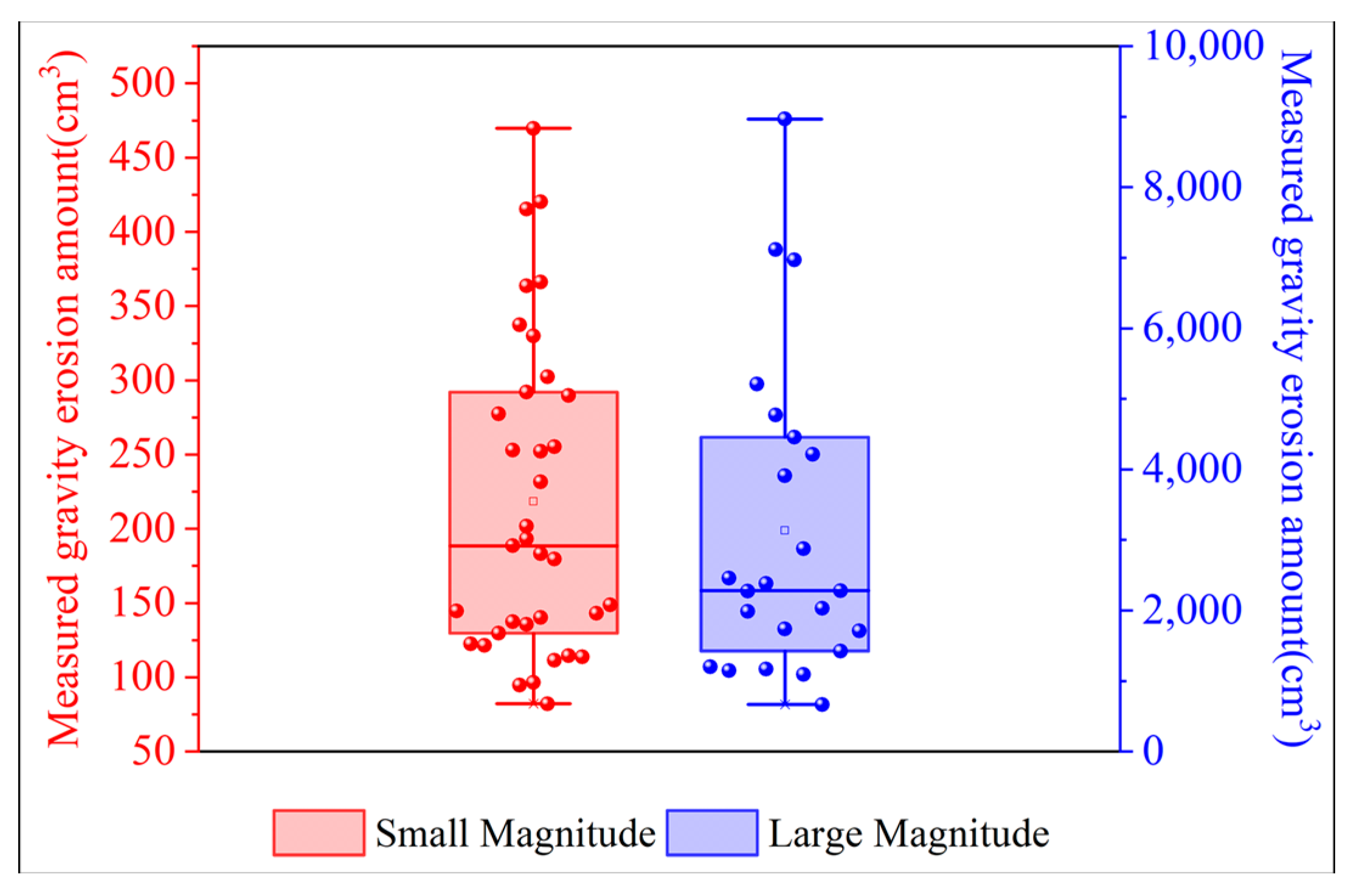
A total of 58 gravity erosion samples were collected from the four experimental plots. The number of large and small gravity erosion samples were 23 and 35, respectively (Figure 10). For the small-magnitude gravity erosion samples, the maximum and minimum values were 469.7 cm3 and 82.1 cm3, respectively, with a mean value of 218.2 cm3. For the large-magnitude samples, the maximum and minimum values were 8967.7 cm3 and 666.0 cm3, respectively, with a mean value of 3132.8 cm3.
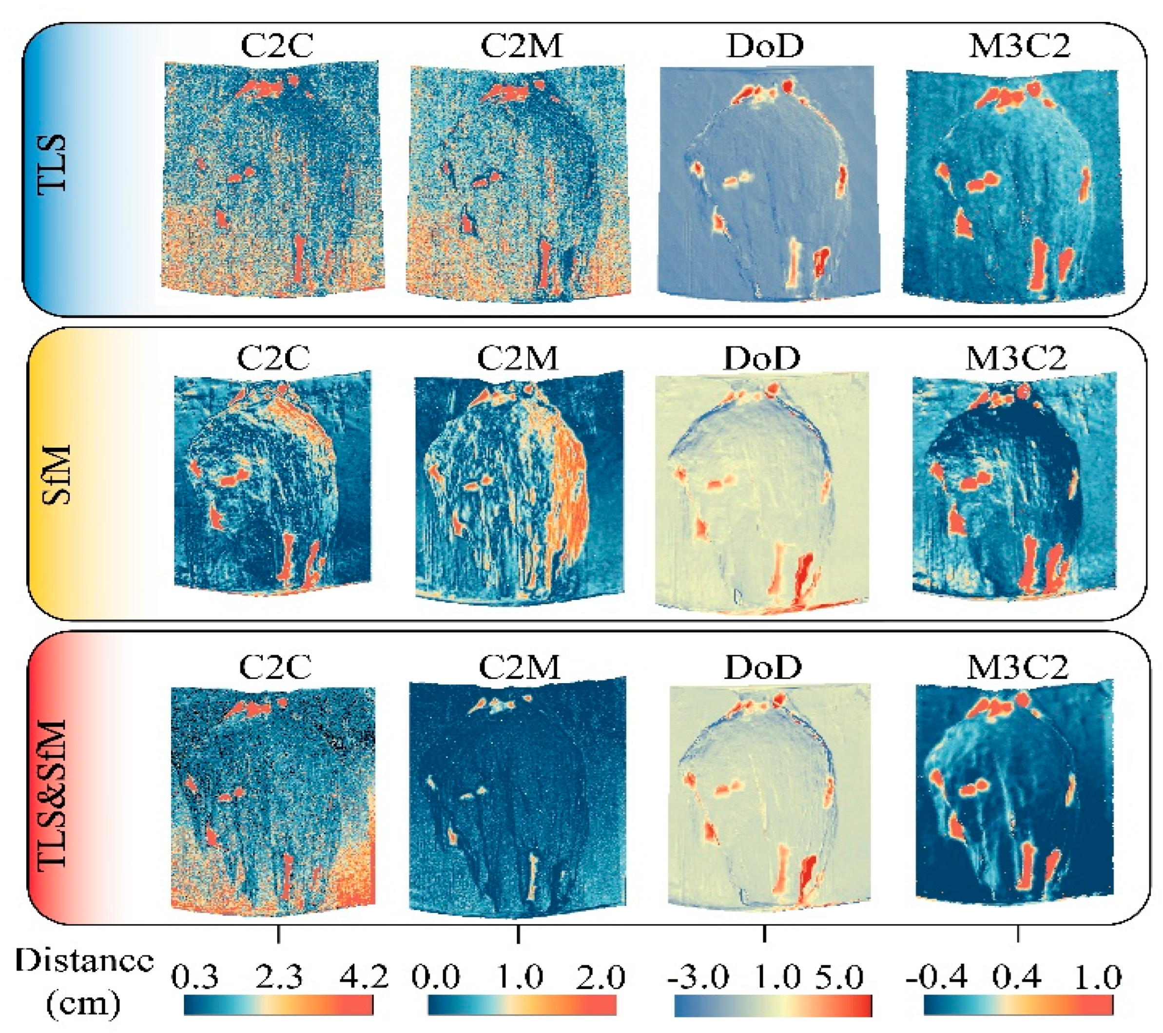
In this study, Plot A was selected as a representative to present the spatial pattern of topographic change on gully slope under the four algorithms (C2C, C2M, DoD and M3C2) (Figure 11). These algorithms could all characterize the distribution information of gravity erosion to a certain extent, but there were certain differences in the boundary of the gravity erosion ranges and the quantification accuracy of terrain changes for different algorithms and various point cloud data. The wider-range high terrain change regions on the sides of the collapse area and the alcove area could be detected in the calculated results of the C2C algorithm and C2M algorithm based on the data derived from SfM. In addition, the boundary of the gravity erosion area is also rather ambiguous, indicating that these two algorithms could not accurately reflect the locations where gravity erosion occurs from the SfM data. The DoD and M3C2 algorithms, by contrast, could display the boundary of the gravity erosion range relatively clearly based on the SfM data. For the data derived from TLS, the C2C algorithm and C2M algorithm had a certain overestimation of terrain changes at the bottom of gully slopes. The DoD and M3C2 algorithms could clearly depict the gravity erosion range, and the quantification accuracy of the terrain change is relatively high on the entire gully slope. The gravity erosion range calculated by the C2C algorithm based on the fused data was relatively clearer in the collapse area than those of the TLS and SfM. However, for the bottom area of the trench, its accuracy was worse than the results from SfM. The range of gravity erosion were also be misclassified by the C2M algorithm plus fused data, and some locations of gravity erosion could not even be identified. In contrast, the boundary of the gravity erosion area calculated by the remaining three algorithms is clear. Especially for the M3C2 algorithm, the of gravity erosion range was clear in the collapse area and the alcove area, and the overall quantification accuracy of gully slope was relatively high.

3.2. Accuracy Comparison of Different Algorithms on Gravity Erosion Quantification

The overall gravity erosion estimated by the four algorithms present obvious differences in quantification accuracy of gravity erosion under the three point cloud data types. For the TLS data, the order of quantification accuracy from low to high for the four detection algorithms was C2C < C2M < DoD < M3C2 in sequence. In particular, the accuracy of the C2C algorithm was much lower than that of the other three algorithms, with the average relative and absolute errors of 2473.16 cm3 and 154.71%, respectively (Table 1). By contrast, the accuracies of the DoD and M3C2 algorithms were close enough to each other, and much higher than that of the other algorithms in gravity erosion quantization, with the mean absolute errors/relative errors of 242.80 cm3 (23.02%) and 427.81 cm3 (22.91%), respectively. For the SfM data, the M3C2 algorithm still had the highest quantification accuracy, while the difference in accuracy from other algorithms was not as obvious as that from the TLS data. The C2M algorithm comes second, with an average relative error of 27.20%. The accuracies of the C2C and M3C2 algorithms were higher based on the fused data of TLS and SfM compared with the accuracy of single-source data. Especially for the C2C algorithm, the relative error was even reduced from 154.71% (C2C algorithm plus TLS) to 29.44% based on fused data. The mean relative error of the M3C2 algorithm plus fused data was even reduced to 14.71%, which was the most accurate among all the algorithms and data sources.
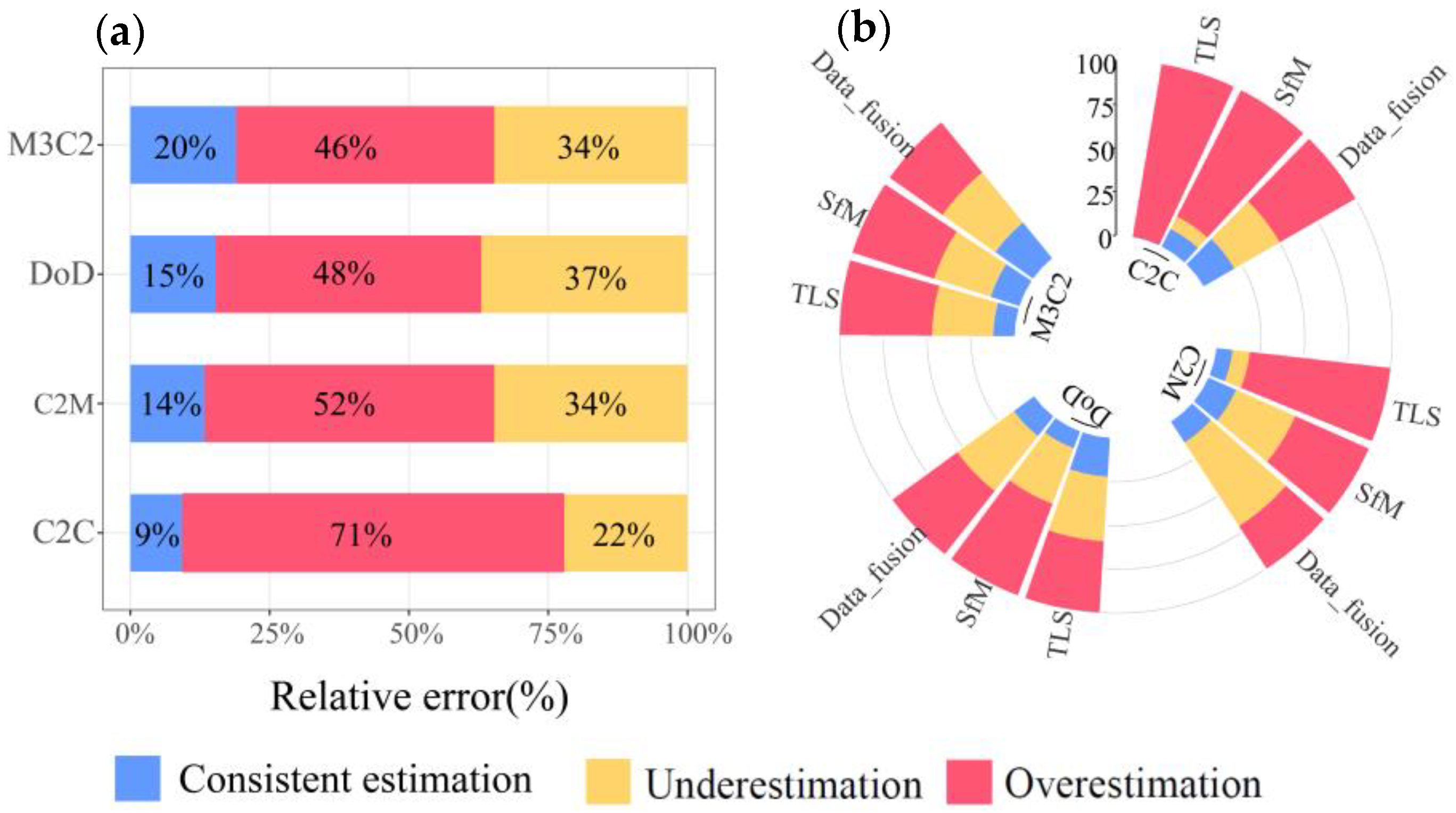
The consistency estimation results of gravity erosion samples by the four algorithms are determined based on relative error (Figure 12a). The results show that the overestimation (OE) ratio, underestimation (UE) ratio and consistent estimation (CE) ratio of various algorithms exhibited differences. The CE ratio of gravity erosion samples quantification based on the M3C2 algorithm is obviously better than that of the remaining three algorithms, reaching 20%. In contrast, the accuracy rate of the C2C algorithm showed the lowest percentage of 9%. The four algorithms all tended to overestimate the gravity erosion amount. Specially, the overestimation (OE) ratio of the C2C algorithm even reached 71%. The underestimation proportion of the four algorithms was between 22% and 37%.
The proportion of consistent estimation, overestimation and underestimation samples was further assessed under different data sources (Figure 12b). For the M3C2 algorithm, the proportion of CE rate by fused TLS and SfM data was larger than that of the single-source TLS and SfM, reaching 26%. While the TLS had the lowest CE ratio using the same algorithm, accounting for 12%. Similarly, the CE rate of the C2C algorithm based on fused TLS and SfM data was also higher than those of the other data sources. The CE ratio of the C2C algorithm using TLS was almost zero, and the proportion of the OE rate was almost 100%. In contrast, the CE ratio (22%) of the gravity erosion amount calculated by the DoD algorithm based on TLS were obviously higher than that of the SfM data (10%) and fused TLS and SfM data (14%). The CE ratio of the C2M algorithm using the data derived from SfM was 17%, which was higher that the CE ratios of TLS data and fused TLS and SfM data. Additionally, the C2C algorithm combined with the data derived from SfM and TLS, as well as the C2M algorithm plus TLS data, mainly overestimated the gravity erosion amount, whereas the C2M algorithm combined with fused TLS and SfM data had the highest UE ratio of all the algorithms and data sources.

3.3. Accuracy Assessment of Different Gravity Erosion Magnitudes

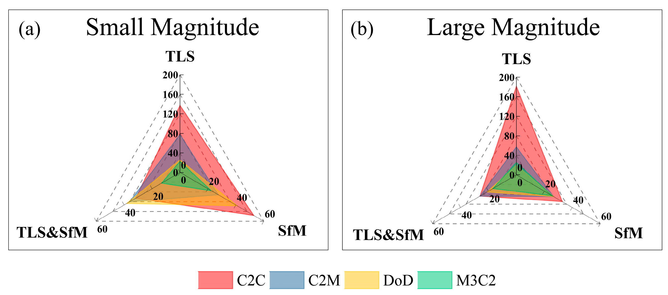
For the small-magnitude gravity erosion samples, the quantification accuracy of the M3C2 algorithm performed the best among different data sources (Figure 13). Among these, the fused TLS and SfM data was the most precise one in the three data sources, with mean relative errors of 13.32%. The calculation accuracy of the four algorithms using the fused TLS and SfM data for the large-magnitude gravity erosion were all relatively high, with the mean relative error ranging from 13.32% to 38.17%. The quantization accuracy of the M3C2 algorithm was basically similar under the two types of magnitudes and obviously larger than that of the other algorithms. By contrast, the mean relative error of the C2C algorithm using the TLS data was the largest for small-magnitude samples (137.28%) and large-magnitude samples (181.25%), while the error is reduced to 31.67% and 26.05% by point cloud fusion, respectively. In addition, the difference in quantitative accuracy of large-magnitude gravity erosion for the C2M, DoD and M3C2 algorithms was relatively small under different data sources. However, there are obvious differences in the quantization accuracy of small-magnitude gravity erosion among different algorithms. Overall, the fused TLS and SfM data combined with the M3C2 algorithm presented good monitoring accuracy on the two magnitudes of gravity erosion.
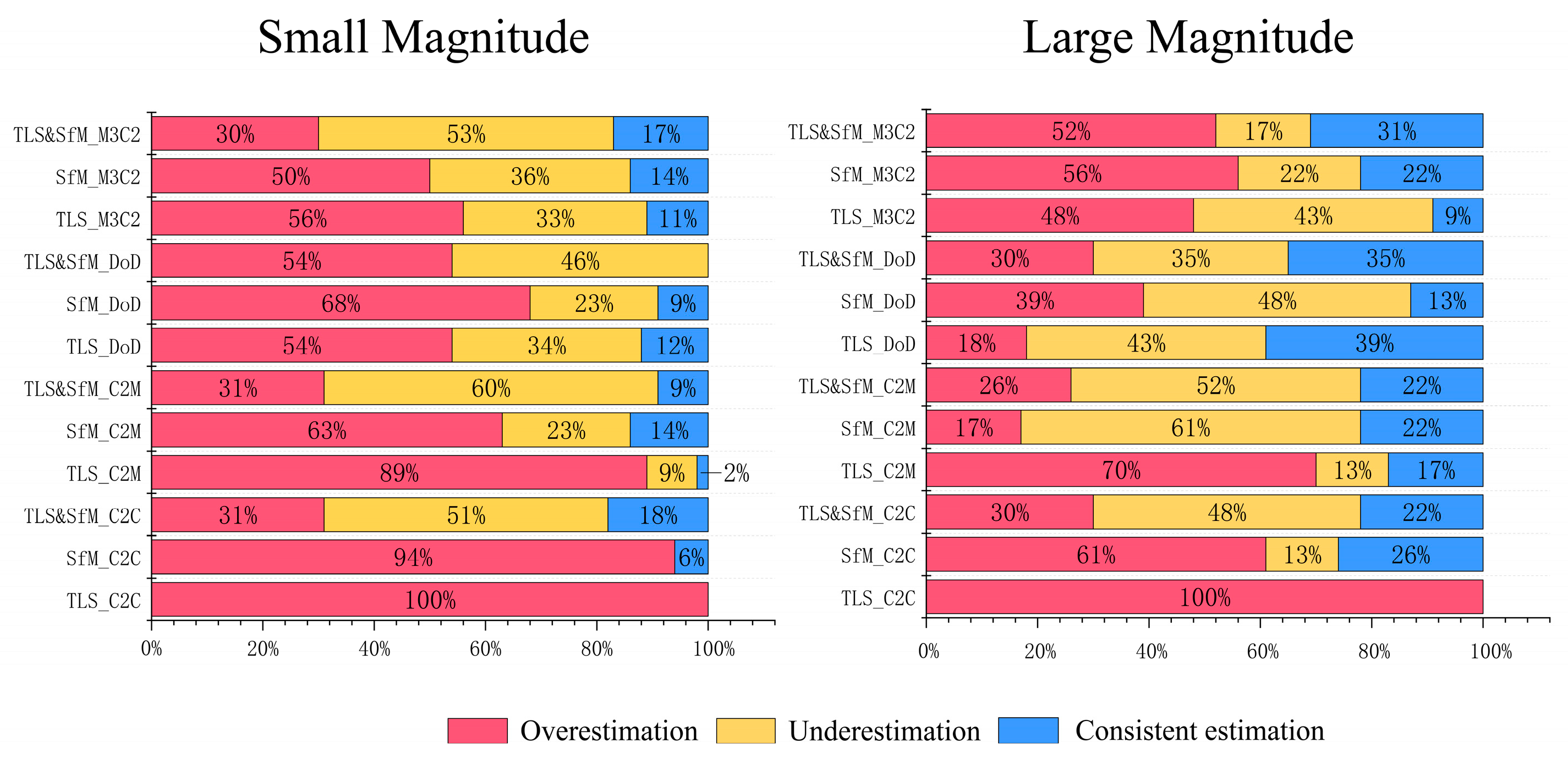
The consistent estimation (CE) rate of large-magnitude samples by different algorithms was generally higher than that of the small-magnitude samples based on the same data sources (Figure 14). For the small-magnitude samples, the CE rate (17%) was the highest using fused TLS and SfM data and M3C2 algorithm. The CE rate of the C2C algorithm was 0% using the single-source data (TLS and SfM), which rises to 17% by data fusion. The CE rate (14%) of gravity erosion quantification based on the C2M algorithm and SfM data was much higher than the other data, while the combination of DoD algorithm and TLS data showed the larger CE rate at 11%. Moreover, the C2C (51% of the samples were underestimated), C2M (60% of the samples were underestimated) and M3C2 (53% of the samples were underestimated) combined fused data tended to underestimate gravity erosion amount, while the combination of the remaining data types and algorithms tended to overestimate erosion volume. Especially, a combination of C2C and TLS data/SfM data produced the highest percentage of overestimation (100% and 94%, respectively). For the large-magnitude samples, the C2C plus TLS data/SfM data also yielded the relatively high overestimation rates of 100% and 61%, respectively. The M3C2 algorithm plus TLS data yielded the highest CE rate (39%) among all the algorithms at the large magnitude, which even exceeds the CE ratio of corresponding fused data. Similarly, the accuracy of C2C algorithms and SfM also exceeded the accuracy of C2C plus fused data. In contrast, the CE ratios (31%) of M3C2 algorithm combined with fused data was higher than that of SfM data (22%) and TLS data (9%). Moreover, the C2M algorithm plus SfM data/fused data tended to seriously underestimate the gravity erosion, with underestimated samples accounting for 61% and 52% of the total, respectively, whereas the C2M algorithm plus TLS tended to overestimate erosion volume, with underestimated samples accounting for 70% of the total.

3.4. Quantification Accuracy of Different Algorithms on Gravity Erosion Under Different Geomorphic Units

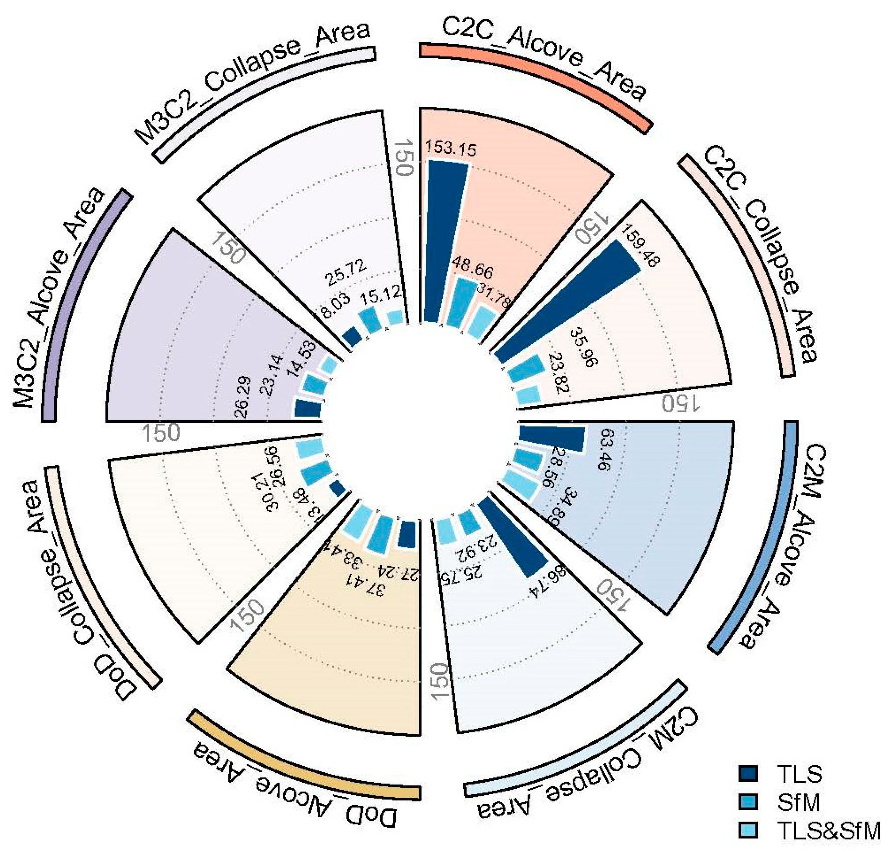
The quantization accuracy of DoD algorithm based on the data derived by TLS perform best in the collapse area, with a mean relative error of 13.48% (Figure 15). The C2C plus TLS data yielded the largest mean relative error (159.48%). In contrast, the C2C plus fused data presented had a relatively low mean relative error (23.82%), which was much lower than that of C2C plus TLS data/SfM data. For the alcove area, the highest accuracy was achieved by the M3C2 algorithm plus fused data, the relative error reached 14.53%. Similarly to the collapse area, the C2C plus TLS data gave the worst quantification accuracy, with a mean relative error of 153.15%. Additionally, the mean relative error of C2M plus TLS data was all relatively high in both the collapse area (86.74%) and the alcove area (63.46%). This were apparently higher than that of the C2M plus SfM data/fused data. Overall, the M3C2/DoD method and various data sources could produce relatively higher quantification accuracy than other strategies under different geomorphic units. Specifically, the DoD algorithm plus TLS data was suitable for quantifying gravity erosion in collapse areas, while the M3C2 algorithm plus TLS data performed better in alcove area.

4. Discussion

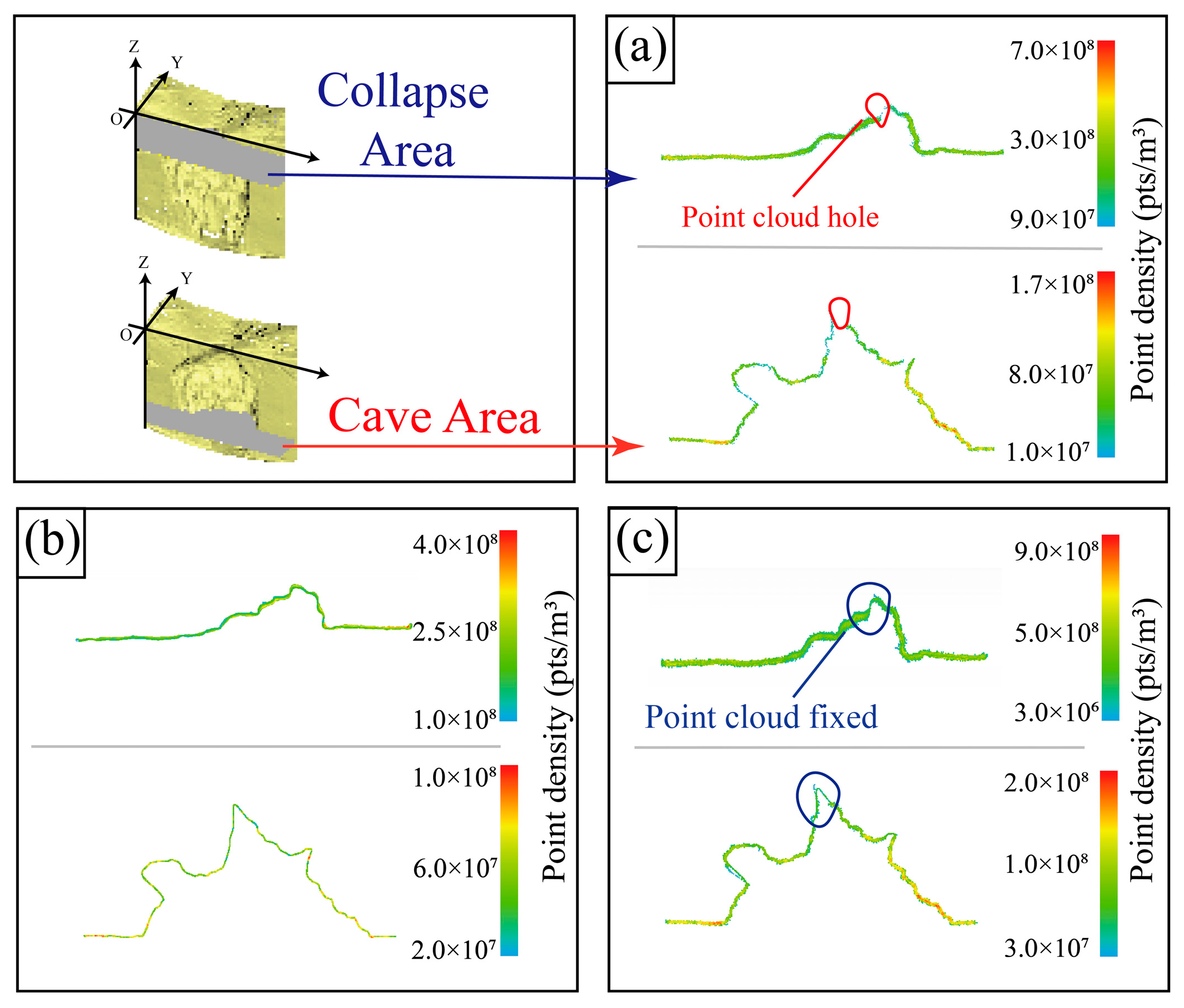
Our study found that the accuracy of most of the fused data was generally higher than that of the single-source data (Table 1). This is because the blocking of vegetation or terrain as well as the light factor will affect the accuracy of single data source, especially for the complex terrain areas [53,54]. This will inevitably produce holes or sparse point cloud areas (Figure 16), thereby affecting the quantization accuracy of the different algorithms. The fused point cloud data can compensate to some extent for the sparse or empty areas in the single-source point cloud data [55]. Moreover, the increase in point cloud density resulting from data fusion is also an important factor affecting the calculation accuracy of gravity erosion. Some other studies also found that the fused data of LiDAR and photogrammetry performed much better in gravity erosion quantization than single-source data based on the field survey results [55,56]. This is consistent with our findings. In addition, the discrepancy in quantization accuracy of gravity erosion was detected between the four algorithms for different terrain units of the gully slope (i.e., collapse areas and caves areas). The DoD algorithm plus TLS was subject to the lowest mean relative errors (13.48%) in the collapse area. In contrast, the quantification accuracy of the M3C2 algorithm in the alcove area was higher than that of DoD, which is inconsistent with the accuracy results of the collapse area. Compared with alcove areas (characterized by terrain mutation areas and complex terrain areas such as both sides of the collapse area), the terrain of the collapse area is relatively simple. Previous researchers showed that the DoD algorithm worked poorly in complex terrain because the problem of elevation overlap cannot be completely avoided [57,58,59], whereas the M3C2 algorithm effectively avoids the repetitive projection issue of the DoD algorithm [60]. Hence, the accuracy of this algorithm is slightly higher than that of the DoD in the alcove area.
In this study, the four change detection algorithms could all detect the locations where gravity erosion occurred partly (Figure 11). Among these, the C2C and C2M could hardly clearly determine the spatial location of gravity erosion in areas with abrupt terrain changes (e.g., collapse area in Figure 11) in comparison. This is because the two algorithms need to detect the closest points in the comparison cloud to the points/triangles in the reference cloud. However, the determined nearest point may not be consistent with the actual direction of change due to the drastically changing erosive terrain on the gully slope, thereby leading to a misjudgment of terrain changes [44,56,61]. Thus, the two methods may not suitable for the terrain changes monitoring that undergo dramatic change on the small scale. The DoD algorithm is one of the most commonly used algorithms for the terrain changes monitoring in geospatial studies. Quantifying the terrain change volume using the DoD algorithm is relatively simple. However, there are limitations when dealing with complex terrain due to the issue of projection overlap and terrain detail blur problems [59]. In contrast, the M3C2 algorithm is used to monitor subtle terrain changes and is suitable for relatively complex terrain [60]. This is consistent with our findings that the distribution range of gravity erosion and the terrain change characteristics derived from M3C2 were superior to those of the other algorithms. Especially for the relatively flat area of the gully area, the detection accuracy of terrain change based on the M3C2 and DoD algorithms was obviously higher. Similarly, our results demonstrated that the M3C2 and DoD algorithms can relatively well quantify the gravity erosion amount under different data sources. The mean relative error was even reduced to 16.66% based on the M3C2 algorithms plus fused data. This is consistent with the findings of some previous studies [42,60], which showed that M3C2 is more suitable for small-scale gravity erosion monitoring on areas with complex terrain. In addition, extremely poor quantification results on gravity erosion were produced by the C2C based on the single-source data (i.e., TLS and SfM), the mean relative error even reached 155.04% based on the TLS data. However, the accuracy of quantitative results was sharply enhanced when fused data was adopted, even surpassing the C2M and DoD algorithm. This might be attributed to the fact that the C2C algorithm was relatively sensitive to the density of the point cloud [62]. With the fusion of the point clouds, the density of point clouds increases greatly (Figure 16), and the quantization accuracy also rises accordingly.

5. Conclusions

In this study, runoff scouring experiments were conducted to obtain the critical terrain where gravity erosion occurs on runoff plots of a natural slope–gully system. Then, the gravity erosion at different locations of the gully slope was removed artificially, and accurate weighing was carried out as the true value. The gravity erosion amount was estimated using four terrain change detection algorithms (DoD, C2C, C2M and M3C2) based on the high-precision topographic data (TLS, SfM and the fusion of single-scan TLS and SfM). Finally, the quantification results of different data sources and change detection algorithms were compared under different terrain features and different magnitudes. The results showed that the M3C2 algorithm could better identify the contour information of the gravity erosion area under different types of point cloud data. Meanwhile, the overall quantification accuracy of the M3C2 algorithm plus fused data was the highest among all the algorithms and data sources, with the mean relative and absolute error being 14.71% and 273.83 cm3, respectively. The fused TLS and SfM data combined with the M3C2 algorithm yielded a good monitoring accuracy on the two magnitudes of gravity erosion. The DoD algorithm plus TLS data might be suitable for quantifying gravity erosion in collapse areas, while the M3C2 algorithm plus TLS data performed better in the alcove area. Our study provides technical support for gravity erosion monitoring on slopes with complex terrain as well as for facilitating gully erosion control.

Author Contributions

Conceptualization, J.H. and P.L.; methodology, J.H.; validation, J.H. and P.L.; formal analysis, H.F.; investigation, J.H., H.F. and J.W.; resources, L.Y. and J.W.; data curation, J.H. and P.L.; writing—original draft preparation, J.H., H.F.; writing—review and editing, J.H. and P.L.; visualization, H.F.; supervision, P.L.; project administration, P.L.; funding acquisition, P.L. All authors have read and agreed to the published version of the manuscript.

Funding

This research was funded by the National Natural Science Foundation of China (U2243211).

Data Availability Statement

Please contact Pengfei Li (pengfeili@xust.edu.cn) for access to the data.

Conflicts of Interest

The authors declare no conflicts of interest.

References

  1. Xu, X.-Z.; Liu, Z.-Y.; Xiao, P.-Q.; Guo, W.-Z.; Zhang, H.-W.; Zhao, C.; Yan, Q. Gravity erosion on the steep loess slope: Behavior, trigger and sensitivity. CATENA 2015, 135, 231–239. [Google Scholar] [CrossRef]
  2. Xu, X.-Z.; Zhang, H.-W.; Wang, W.-L.; Zhao, C.; Yan, Q. Quantitative monitoring of gravity erosion using a novel 3D surface measuring technique: Validation and case study. Nat. Hazards 2015, 75, 1927–1939. [Google Scholar] [CrossRef]
  3. Kuhn, C.E.S.; Reis, F.A.G.V.; Zarfl, C.; Grathwohl, P.J.N.H. Ravines and gullies, a review about impact valuation. Nat. Hazards 2023, 117, 597–624. [Google Scholar] [CrossRef]
  4. Larsen, I.J.; Montgomery, D.R.; Korup, O. Landslide erosion controlled by hillslope material. Nat. Geosci. 2010, 3, 247–251. [Google Scholar] [CrossRef]
  5. Borrelli, P.; Robinson, D.A.; Panagos, P.; Lugato, E.; Yang, J.E.; Alewell, C.; Wuepper, D.; Montanarella, L.; Ballabio, C. Land use and climate change impacts on global soil erosion by water (2015–2070). Proc. Natl. Acad. Sci. USA 2020, 117, 21994–22001. [Google Scholar] [CrossRef] [PubMed]
  6. Peñuela, A.; Hayas, A.; Infante-Amate, J.; Ruiz-Montes, P.; Temme, A.; Reimann, T.; Peña-Acevedo, A.; Vanwalleghem, T. A multi-millennial reconstruction of gully erosion in two contrasting Mediterranean catchments. CATENA 2023, 220, 106709. [Google Scholar] [CrossRef]
  7. Gariano, S.L.; Guzzetti, F. Landslides in a changing climate. Earth-Sci. Rev. 2016, 162, 227–252. [Google Scholar] [CrossRef]
  8. Li, L.; Nearing, M.A.; Nichols, M.H.; Polyakov, V.O.; Cavanaugh, M.L. Using terrestrial LiDAR to measure water erosion on stony plots under simulated rainfall. Earth Surf. Proc. Land. 2020, 45, 484–495. [Google Scholar] [CrossRef]
  9. Mouyen, M.; Masson, F.; Hwang, C.; Cheng, C.-C.; Le Moigne, N.; Lee, C.W.; Kao, R.; Hsieh, W.-C. Erosion effects assessed by repeated gravity measurements in southern Taiwan. Geophys. J. Int. 2013, 192, 113–136. [Google Scholar] [CrossRef]
  10. Slee, A.J.; McIntosh, P.D.; Barrows, T.T. Using 36Cl exposure dating to date mass movement and assess land stability on the Nicholas Range, Tasmania. Landslides 2017, 14, 2147–2154. [Google Scholar] [CrossRef]
  11. Unkel, I.; Ehret, D.; Rohn, J. Recurrence analysis of the mass movement activity at Stambach (Austria) based on radiocarbon dating. Geomorphology 2013, 190, 103–111. [Google Scholar] [CrossRef]
  12. Zhang, N.; Yang, J.; Xing, W.; Liu, X.; Sheng, F.; Zhao, W.; Zhang, Z.; Tian, Z.; Chen, R. Isotope tracer study of soil erosion in a typical sub-watershed in the eastern Tianshan Mountains, China. J. Environ. Radioact. 2025, 285, 107667. [Google Scholar] [CrossRef]
  13. Zhu, T. Gully and tunnel erosion in the hilly Loess Plateau region, China. Geomorphology 2012, 153, 144–155. [Google Scholar] [CrossRef]
  14. Abedini, M.; Said, M.A.M.; Ahmad, F. Effectiveness of check dam to control soil erosion in a tropical catchment (The Ulu Kinta Basin). CATENA 2012, 97, 63–70. [Google Scholar] [CrossRef]
  15. Rieke-Zapp, D.H.; Nearing, M.A. Digital close range photogrammetry for measurement of soil erosion. Photogramm. Rec. 2005, 20, 69–87. [Google Scholar] [CrossRef]
  16. Zhu, T.; Xu, X.; Zhu, A. Spatial variation in the frequency and magnitude of mass movement in a semiarid, complex-terrain agricultural watershed on the Loess Plateau of China. Land. Degrad. Dev. 2019, 30, 1095–1106. [Google Scholar] [CrossRef]
  17. Di Stefano, C.; Ferro, V.; Pampalone, V.; Sanzone, F. Field investigation of rill and ephemeral gully erosion in the Sparacia experimental area, South Italy. CATENA 2013, 101, 226–234. [Google Scholar] [CrossRef]
  18. Xia, J.; Zhang, L.; Huang, X.; Lu, X.; Ge, P.; Wei, Y.; Cai, C. Photogrammetric Technique-Based Quantitative Measuring of Gravity Erosion on Steep Slopes in Laboratory: Accuracy and Application. Water 2023, 15, 2584. [Google Scholar] [CrossRef]
  19. Barnes, N.; Luffman, I.; Nandi, A. Gully erosion and freeze-thaw processes in clay-rich soils, northeast Tennessee, USA. GeoResJ 2016, 9, 67–76. [Google Scholar] [CrossRef]
  20. Vandekerckhove, L.; Poesen, J.; Wijdenes, D.O.; Gyssels, G. Short-term bank gully retreat rates in Mediterranean environments. CATENA 2001, 44, 133–161. [Google Scholar] [CrossRef]
  21. Gholami, V.; Sahour, H.; Amri, M.A.H. Soil erosion modeling using erosion pins and artificial neural networks. CATENA 2021, 196, 104902. [Google Scholar] [CrossRef]
  22. Nouwakpo, S.K.; Weltz, M.A.; McGwire, K. Assessing the performance of structure-from-motion photogrammetry and terrestrial LiDAR for reconstructing soil surface microtopography of naturally vegetated plots. Earth Surf. Proc. Land. 2016, 41, 308–322. [Google Scholar] [CrossRef]
  23. Betts, H.D.; Trustrum, N.A.; Rose, R.C.D. Geomorphic changes in a complex gully system measured from sequential digital elevation models, and implications for management. Earth Surf. Proc. Land. 2003, 28, 1043–1058. [Google Scholar] [CrossRef]
  24. Zhang, S.; Wang, X.; Xiao, Z.; Qu, F.; Wang, X.; Li, Y.; Aurangzeib, M.; Zhang, X.; Liu, X. Quantitative studies of gully slope erosion and soil physiochemical properties during freeze-thaw cycling in a Mollisol region. Sci. Total Environ. 2020, 707, 136191. [Google Scholar] [CrossRef]
  25. Chico, G.; Clutterbuck, B.; Midgley, N.; Labadz, J. Application of terrestrial laser scanning to quantify surface changes in restored and degraded blanket bogs. Mires Peat 2019, 24, 14. [Google Scholar]
  26. Song, W.; Liu, P.; Yang, M.; Xue, Y. Using REE Tracers to Measure Sheet Erosion Changing to Rill Erosion. J. Rare Earth 2003, 21, 587–590. [Google Scholar]
  27. Webster, C.; Westoby, M.; Rutter, N.; Jonas, T. Three-dimensional thermal characterization of forest canopies using UAV photogrammetry. Remote Sens. Environ. 2018, 209, 835–847. [Google Scholar] [CrossRef]
  28. Jiang, Y.; Shi, H.; Wen, Z.; Guo, M.; Zhao, J.; Cao, X.; Fan, Y.; Zheng, C. The dynamic process of slope rill erosion analyzed with a digital close range photogrammetry observation system under laboratory conditions. Geomorphology 2020, 350, 106893. [Google Scholar] [CrossRef]
  29. Iglhaut, J.; Cabo, C.; Puliti, S.; Piermattei, L.; O’Connor, J.; Rosette, J. Structure from motion photogrammetry in forestry: A review. Curr. For. Rep. 2019, 5, 155–168. [Google Scholar] [CrossRef]
  30. Chen, G.; Ozelkan, E.; Singh, K.K.; Zhou, J.; Brown, M.R.; Meentemeyer, R.K. Uncertainties in mapping forest carbon in urban ecosystems. J. Environ. Manag. 2017, 187, 229–238. [Google Scholar] [CrossRef] [PubMed]
  31. Okyay, U.; Telling, J.; Glennie, C.L.; Dietrich, W.E. Airborne lidar change detection: An overview of Earth sciences applications. Earth-Sci. Rev. 2019, 198, 102929. [Google Scholar] [CrossRef]
  32. Pfeiffer, J.; Zieher, T.; Rutzinger, M.; Bremer, M.; Wichmann, V. Comparison and time series analysis of landslide displacement mapped by airborne, terrestrial and unmanned aerial vehicle based platforms. ISPRS Ann. Photogramm. Remote Sens. Spat. Inf. Sci. 2019, 4, 421–428. [Google Scholar] [CrossRef]
  33. Kenner, R.; Bühler, Y.; Delaloye, R.; Ginzler, C.; Phillips, M. Monitoring of high alpine mass movements combining laser scanning with digital airborne photogrammetry. Geomorphology 2014, 206, 492–504. [Google Scholar] [CrossRef]
  34. Bitelli, G.; Dubbini, M.; Zanutta, A. Terrestrial laser scanning and digital photogrammetry techniques to monitor landslide bodies. Int. Arch. Photogramm. Remote Sens. Spat. Inf. Sci. 2004, 35, 246–251. [Google Scholar]
  35. Salvini, R.; Francioni, M.; Riccucci, S.; Bonciani, F.; Callegari, I. Photogrammetry and laser scanning for analyzing slope stability and rock fall runout along the Domodossola–Iselle railway, the Italian Alps. Geomorphology 2013, 185, 110–122. [Google Scholar] [CrossRef]
  36. Sestras, P.; Bilașco, Ș.; Roșca, S.; Veres, I.; Ilies, N.; Hysa, A.; Spalević, V.; Cîmpeanu, S.M. Multi-instrumental approach to slope failure monitoring in a landslide susceptible newly built-up area: Topo-Geodetic survey, UAV 3D modelling and ground-penetrating radar. Remote Sens. 2022, 14, 5822. [Google Scholar] [CrossRef]
  37. Stumpf, A.; Malet, J.-P.; Allemand, P.; Pierrot-Deseilligny, M.; Skupinski, G. Ground-based multi-view photogrammetry for the monitoring of landslide deformation and erosion. Geomorphology 2015, 231, 130–145. [Google Scholar] [CrossRef]
  38. Girardeau-Montaut, D.; Roux, M.; Marc, R.; Thibault, G. Change detection on points cloud data acquired with a ground laser scanner. Int. Arch. Photogramm. Remote Sens. Spat. Inf. Sci. 2005, 36, W19. [Google Scholar]
  39. Martínez-Espejo Zaragoza, I.; Caroti, G.; Piemonte, A.; Riedel, B.; Tengen, D.; Niemeier, W. Structure from motion (SfM) processing of UAV images and combination with terrestrial laser scanning, applied for a 3D-documentation in a hazardous situation. Geomat. Nat. Haz. Risk 2017, 8, 1492–1504. [Google Scholar] [CrossRef]
  40. Williams, R. DEMs of difference. Geomorphol. Tech. 2012, 2, 1–17. [Google Scholar]
  41. Abdelazeem, M.; Elamin, A.; Afifi, A.; El-Rabbany, A. Multi-sensor point cloud data fusion for precise 3D mapping. Egypt. J. Remote Sens. Space Sci. 2021, 24, 835–844. [Google Scholar] [CrossRef]
  42. Lague, D.; Brodu, N.; Leroux, J. Accurate 3D comparison of complex topography with terrestrial laser scanner: Application to the Rangitikei canyon (NZ). Isprs J. Photogramm. 2013, 82, 10–26. [Google Scholar] [CrossRef]
  43. Wheaton, J.M.; Brasington, J.; Darby, S.E.; Sear, D.A. Accounting for uncertainty in DEMs from repeat topographic surveys: Improved sediment budgets. Earth Surf. Proc. Land. 2010, 35, 136–156. [Google Scholar] [CrossRef]
  44. Nourbakhshbeidokhti, S.; Kinoshita, A.M.; Chin, A.; Florsheim, J.L. A workflow to estimate topographic and volumetric changes and errors in channel sedimentation after disturbance. Remote Sens. 2019, 11, 586. [Google Scholar] [CrossRef]
  45. Mukupa, W.; Roberts, G.W.; Hancock, C.M.; Al-Manasir, K. A review of the use of terrestrial laser scanning application for change detection and deformation monitoring of structures. Surv. Rev. 2017, 49, 99–116. [Google Scholar] [CrossRef]
  46. Palmeri, V.; Di Stefano, C.; Guida, G.; Nicosia, A.; Ferro, V. Monitoring the temporal evolution of a Sicilian badland area by unmanned aerial vehicles. Geomorphology 2024, 466, 109443. [Google Scholar] [CrossRef]
  47. Shi, P.; Zhang, Y.; Zhang, Y.; Yu, Y.; Li, P.; Li, Z.; Xiao, L.; Xu, G.; Zhu, T. Land-use types and slope topography affect the soil labile carbon fractions in the Loess hilly-gully area of Shaanxi, China. Arch. Agron. Soil Sci. 2020, 66, 638–650. [Google Scholar] [CrossRef]
  48. Zhang, Z. Iterative Closest Point (ICP). In Computer Vision: A Reference Guide; Springer: Berlin/Heidelberg, Germany, 2021; pp. 718–720. [Google Scholar]
  49. Sui, H.; Asaba, K.; Sakai, K.; Miyanaga, S.; Cui, Y. Assessment of C2C-based point cloud comparison errors based on distribution characteristics of tunnel point clouds. Int. J. Remote Sens. 2025, 46, 2646–2664. [Google Scholar] [CrossRef]
  50. Cook, K.L. An evaluation of the effectiveness of low-cost UAVs and structure from motion for geomorphic change detection. Geomorphology 2017, 278, 195–208. [Google Scholar] [CrossRef]
  51. Seo, H.; Zhao, Y.; Chen, C. Displacement estimation error in laser scanning monitoring of retaining structures considering roughness. Sensors 2021, 21, 7370. [Google Scholar] [CrossRef]
  52. Lane, S.N.; Westaway, R.M.; Murray Hicks, D. Estimation of erosion and deposition volumes in a large, gravel-bed, braided river using synoptic remote sensing. Earth Surf. Proc. Land. 2003, 28, 249–271. [Google Scholar] [CrossRef]
  53. Su, J.; Bork, E. Influence of vegetation, slope, and lidar sampling angle on DEM accuracy. Photogramm. Eng. Remote Sens. 2006, 72, 1265–1274. [Google Scholar] [CrossRef]
  54. Zhang, R.; Schneider, D.; Strauß, B. Generation and comparison of TLS and SFM based 3d models of solid shapes in hydromechanic research. Int. Arch. Photogramm. Remote Sens. Spat. Inf. Sci. 2016, 41, 925–929. [Google Scholar] [CrossRef]
  55. Ji, H.; Luo, X. 3D scene reconstruction of landslide topography based on data fusion between laser point cloud and UAV image. Environ. Earth Sci. 2019, 78, 534. [Google Scholar] [CrossRef]
  56. Yan, L.; Li, P.; Hu, J.; Li, D.; Dan, Y.; Bai, X.; Liu, L.; Gao, J.; Dang, T.; Dang, W. Monitoring small-scale mass movement using unmanned aerial vehicle remote sensing techniques. CATENA 2024, 238, 107885. [Google Scholar] [CrossRef]
  57. Croke, J.; Todd, P.; Thompson, C.; Watson, F.; Denham, R.; Khanal, G. The use of multi temporal LiDAR to assess basin-scale erosion and deposition following the catastrophic January 2011 Lockyer flood, SE Queensland, Australia. Geomorphology 2013, 184, 111–126. [Google Scholar] [CrossRef]
  58. Le Mauff, B.; Juigner, M.; Ba, A.; Robin, M.; Launeau, P.; Fattal, P. Coastal monitoring solutions of the geomorphological response of beach-dune systems using multi-temporal LiDAR datasets (Vendée coast, France). Geomorphology 2018, 304, 121–140. [Google Scholar] [CrossRef]
  59. Yang, X.; Hu, J.; Li, P.; Gao, C.; Latifi, H.; Bai, X.; Gao, J.; Dang, T.; Tang, F. SCCD: A slicing algorithm for detecting geomorphic changes on topographically complex areas based on 3D point clouds. Remote Sens. Environ. 2024, 303, 114022. [Google Scholar] [CrossRef]
  60. Gao, C.; Li, P.; Hu, J.; Yan, L.; Latifi, H.; Yao, W.; Hao, M.; Gao, J.; Dang, T.; Zhang, S. Development of gully erosion processes: A 3D investigation based on field scouring experiments and laser scanning. Remote Sens. Environ. 2021, 265, 112683. [Google Scholar] [CrossRef]
  61. Jafari, B.; Khaloo, A.; Lattanzi, D. Deformation tracking in 3D point clouds via statistical sampling of direct cloud-to-cloud distances. J. Nondestruct. Eval. 2017, 36, 65. [Google Scholar] [CrossRef]
  62. Meinen, B.U.; Robinson, D.T. Mapping erosion and deposition in an agricultural landscape: Optimization of UAV image acquisition schemes for SfM-MVS. Remote Sens. Environ. 2020, 239, 111666. [Google Scholar] [CrossRef]
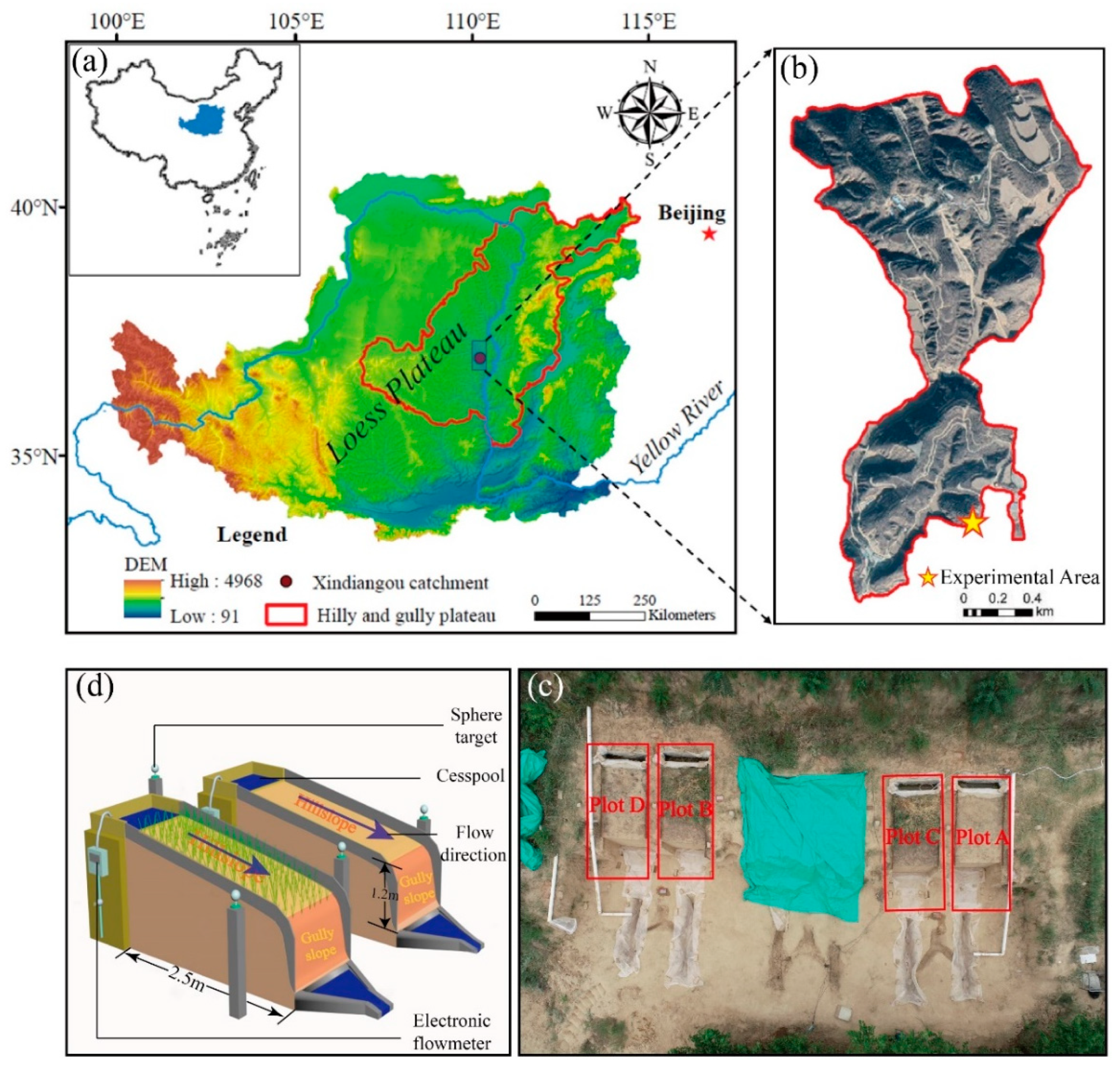
Figure 1. Study site and the experimental design. (a) Geographical location of the hilly–gully area on the loess plateau; (b) Schematic map of the Xindiangou watershed; (c) Top view of the experimental plot; (d) Three-dimensional schematic of the experimental plot.
Water 17 02309 g001
Figure 2. Layout of experimental area.
Water 17 02309 g002
Figure 3. The illustration of collapse area and alcove area on the gully slope.
Water 17 02309 g003
Figure 4. Locations of gravity erosion during the simulation experiments. (a) Small-magnitude gravity erosion; (b) Large-magnitude gravity erosion. (Note: The numbers in the figure represent the locations of different gravity erosion samples).
Water 17 02309 g004
Figure 5. Different types of point cloud data. (a) Single scan TLS point cloud; (b) SfM point cloud; (c) Fused data of Single scan TLS and SfM.
Water 17 02309 g005
Figure 6. Illustration of the C2C algorithm.
Water 17 02309 g006
Figure 7. Illustration of the C2M algorithm.
Water 17 02309 g007
Figure 8. Illustration of DoD algorithm.
Water 17 02309 g008
Figure 9. Illustration of M3C2 algorithm. (a) Reference point cloud and comparison point cloud; (b) Cylinder creating; (c) Distance calculation; (d) positive and negative terrain changes determining; (e) M3C2 distance.
Water 17 02309 g009
Figure 10. The statistical distribution of measured gravitational erosion amounts.
Water 17 02309 g010
Figure 11. The spatial pattern of topographic change on the gully slope.
Water 17 02309 g011
Figure 12. Percentage of consistent estimation, overestimation or underestimation of gravity erosion. (a) Overall relative error; (b) Relative error of different algorithms and data sources.
Water 17 02309 g012
Figure 13. Relative errors of estimated gravity erosion amount under different magnitudes. (a) Small magnitude; (b) Large magnitude.
Water 17 02309 g013
Figure 14. Percentage of overestimation, underestimation, and consistent estimation of gravity erosion at different magnitudes.
Water 17 02309 g014
Figure 15. The relative error of gravity erosion samples in different terrain units.
Water 17 02309 g015
Figure 16. The spatial characteristics of point cloud under different terrain units. (a) TLS point cloud data. (b) SfM point cloud data. (c) Fused TLS and SfM data.
Water 17 02309 g016
Table 1. Accuracy comparison of gravity erosion quantification based on different algorithms and data sources.
AlgorithmData SourceAbsolute Error (cm3)Relative Error (%)
MaxMinMeanMaxMinMean
C2CTLS18209.3551.962473.16342.9716.69154.71
SfM3345.047.05358.90140.370.1444.94
TLS and SfM2274.660.67257.67208.360.5229.44
C2MTLS5621.161.36666.69272.930.7769.68
SfM2778.891.09328.39103.800.8127.20
TLS and SfM2261.472.41266.71207.150.1132.21
DoDTLS1974.611.36242.80135.070.6123.02
SfM1515.842.53275.38115.750.9035.30
TLS and SfM2881.186.54263.61133.430.2731.40
M3C2TLS5611.000.20427.8181.090.0122.91
SfM4726.900.40354.54102.780.1623.85
TLS and SfM3306.201.85273.8365.330.0914.71
Disclaimer/Publisher’s Note: The statements, opinions and data contained in all publications are solely those of the individual author(s) and contributor(s) and not of MDPI and/or the editor(s). MDPI and/or the editor(s) disclaim responsibility for any injury to people or property resulting from any ideas, methods, instructions or products referred to in the content.