Article

Integrated Flushing and Corrosion Control Measures to Reduce Lead Exposure in Households with Lead Service Lines †

1
Industrial Chair in Drinking Water, Department of Civil, Geological and Mining Engineering, Polytechnique Montreal, Montreal, QC H3C 3A7, Canada
2
KWR Water Research Institute, Groningenhaven 7, 3433 PE Nieuwegein, The Netherlands
3
Delft University of Technology, P.O. Box 5, 2600 AA Delft, The Netherlands
*
Author to whom correspondence should be addressed.
This paper is an extended version of our paper published in Hatam, F.; Blokker, E.; Prévost, M. Evaluation of flushing and corrosion control to lower lead levels at the taps in households with lead service lines. In Proceedings of 19th Computing and Control for the Water Industry Conference (CCWI), Leicester, UK, 4–7 September 2023.
Water 2025, 17(15), 2297; https://doi.org/10.3390/w17152297 (registering DOI)
Submission received: 11 June 2025 / Revised: 25 July 2025 / Accepted: 30 July 2025 / Published: 2 August 2025

Abstract

The quality of water in households can be affected by plumbing design and materials, water usage patterns, and source water quality characteristics. These factors influence stagnation duration, disinfection residuals, metal release, and microbial activity. In particular, stagnation can degrade water quality and increase lead release from lead service lines. This study employs numerical modeling to assess how combined corrosion control and flushing strategies affect lead levels in household taps with lead service lines under reduced water use. To estimate potential health risks, the U.S. EPA model is used to predict the percentage of children likely to exceed safe blood lead levels. Lead exceedances are assessed based on various regulatory requirements. Results show that exceedances at the kitchen tap range from 3 to 74% of usage time for the 5 µg/L standard, and from 0 to 49% for the 10 µg/L threshold, across different scenarios. Implementing corrosion control treatment in combination with periodic flushing proves effective in lowering lead levels under the studied low-consumption scenarios. Under these conditions, the combined strategy limits lead exceedances above 5 µg/L to only 3% of usage time, with none above 10 µg/L. This demonstrates its value as a practical short-term strategy for households awaiting full pipe replacement. Targeted flushing before peak water use reduces the median time that water remains stagnant in household pipes from 8 to 3 h at the kitchen tap under low-demand conditions. Finally, the risk model indicates that the combined approach can reduce the predicted percentage of children with blood lead levels exceeding 5 μg/dL from 61 to 6% under low water demand.

1. Introduction

Lead sources and public health risks. Lead in drinking water can originate from various sources such as solders, taps, pipe fittings, brass fixtures, and lead service lines [1]. Lead service lines (LSLs) were commonly installed in buildings in many countries including Canada until 1975 [2]. Although their use was banned by then, many of these buildings still have pipes in place. While there is agreement that all lead service lines should be replaced [3], the process remains slow and challenging due to high costs. When present, LSLs can be considered as dominant sources of lead in taps. The harmful effects of lead exposure primarily target the developing brain and nervous systems, posing an increased risk for young children [4]. Lead is a neurotoxin, especially harmful to young children, and even low-level exposure has been associated with higher cardiovascular disease mortality rates in the United States [5]. This is why standards and guidelines for lead in drinking have been improved over time. A new standard of 5 μg/L as the maximum acceptable concentration for total lead in drinking water is now proposed by Health Canada [1] and to be implemented in European countries by 2036 [6].
Conservation and stagnation challenges. Furthermore, water stagnation within buildings can increase by water consumption reduction strategies, contributing to increased lead leaching [7]. Water conservation strategies are increasing in response to regulatory mandates that aim to lower environmental impact, preserving aquatic environments and mitigate water scarcity [8,9,10]. While fully replacing all LSLs can be a time-consuming process and with water conservation programs in place, corrosion control or other mitigation strategies such as flushing are required to reduce the potential risk of exposure to elevated lead levels. Proctor et al. [11] reviewed preventative and remedial strategies to address water quality issues during prolonged stagnation in large buildings due to fully or partially shutdown. The study highlights the health risks associated with stagnant water, including chemical contaminants like lead and copper, as well as microbiological risks from opportunistic pathogens. Salehi et al. [12] investigated seasonal and spatial variations in water quality within a net-zero energy residential building through sampling events and online monitoring records. They identified seasonal and spatial differences in water quality at the service line and across fixtures. Major differences in pH, chlorine residual, organic carbon, total trihalomethanes, select heavy metals, and nitrogen compounds across fixtures were found. Their study emphasized the necessity for models to predict drinking water chemical characteristics at building fixtures and emphasizes the need for innovations in building water sensor technologies.
Modeling lead mitigation under water conservation. Numerical approaches can be useful tools for estimating the typical lead exposure level at the household level, which can then be used as the basis to assess compliance and implement necessary remedial measures. While many studies have utilized numerical tools to assess water quality in distribution systems, some specifically focusing on the performance of these systems in adopting conservation strategies [13,14,15], relatively less research haves used hydraulic models to simulate water quality within buildings. Recently, however, interest has grown in modeling premise plumbing systems, with several studies using EPANET to estimate variation in dissolved lead concentrations in taps [16,17,18,19]. For example, Hatam et al. [19] evaluated the impact of water conservation strategies on dissolved lead concentrations and potential blood lead levels (BLLs) in children, considering various water qualities and lead service lines lengths. However, none of these studies examined the combined effects of flushing and corrosion control treatments on the spatial–temporal variation in lead concentrations, a key novelty of this study.
Water quality modeling under stagnation and flushing conditions. Vizanko et al. [20] employed a hydraulic model to investigate the impact of social distancing measures on spatial changes in water demand and consequently water age within urban water distribution systems during the COVID-19 pandemic. Burkhardt et al. [21] used a Python-based premise plumbing modeling framework to simulate relative water age in single-family homes. The authors showed that increasing pipe diameter or hot water heater volume or using lower flow fixtures can lead to higher relative water ages. Clements et al. [22] quantified the impact of purging on relative water age in premise plumbing systems, demonstrating that larger purge volumes lead to lower water ages, while even small volumes can have a significant effect on age. Despite widespread recommendations for flushing to maintain water quality in buildings, there remains lack of modeling studies assessing its effectiveness under low water usage conditions, particularly in systems with lead service lines, where balancing water conservation and lead exposure presents a critical challenge.
Integrated Exposure Uptake Biokinetic (IEUBK) modeling. Lead is a well-known neurotoxin linked to cardiovascular disease, with children being particularly vulnerable due to their higher gastrointestinal uptake rates compared to adults [23,24]. Children are particularly vulnerable due to their higher uptake rates compared to adults [25,26]. Several recent studies have highlighted the significant role of drinking water in children’s lead exposure. Levallois et al. [27] conducted a controlled LSL epidemiological study reported that dust, water, and paint all significantly contributed to elevated BLLs in 306 children aged 1–5 years in targeted areas of Montreal. More importantly, modeled BLLs using IEUBK were consistent with measured BLLs [28]. Further analysis of the data led to actionable recommendations of flushing as the percentage of children exceeding 5 μg/dL during the warmer summer period could be limited by flushing water at least 5 min before consumption [29]. More recently, Stanek et al. [30] used a combined SHEDS–IEUBK framework with data from 15 U.S. cities and found that residential drinking water contributed approximately 10% to 80% of total lead exposure, with the highest values in formula-fed infants in homes with lead service lines and no corrosion control.
Study scope. Modeling techniques can assist in better defining targeted and effective strategies for mitigating lead exposure risks and conducting compliance evaluations. The combined influence of flushing and corrosion control on spatial and temporal variations in lead levels within premise plumbing systems remains insufficiently explored. To address these challenges, this study used modeling techniques to evaluate the combined effectiveness of flushing and corrosion control measures in reducing lead exposure in households with lead service lines. A simple household drinking water system was simulated, using a stochastic water demand model and a calibrated lead dissolution model based on existing field data in the literature. The analysis focuses on how these interventions influence lead concentrations and relative water age under low water consumption scenarios. Simulated lead levels at the kitchen tap are assessed against various drinking water standards to evaluate the frequency and severity of exceedances under different demand conditions and remedial measures. Finally, the IEUBK model was used to estimate the percentage of children aged 0–84 months predicted to have BLLs exceeding 5 μg/dL.

2. Materials and Methods

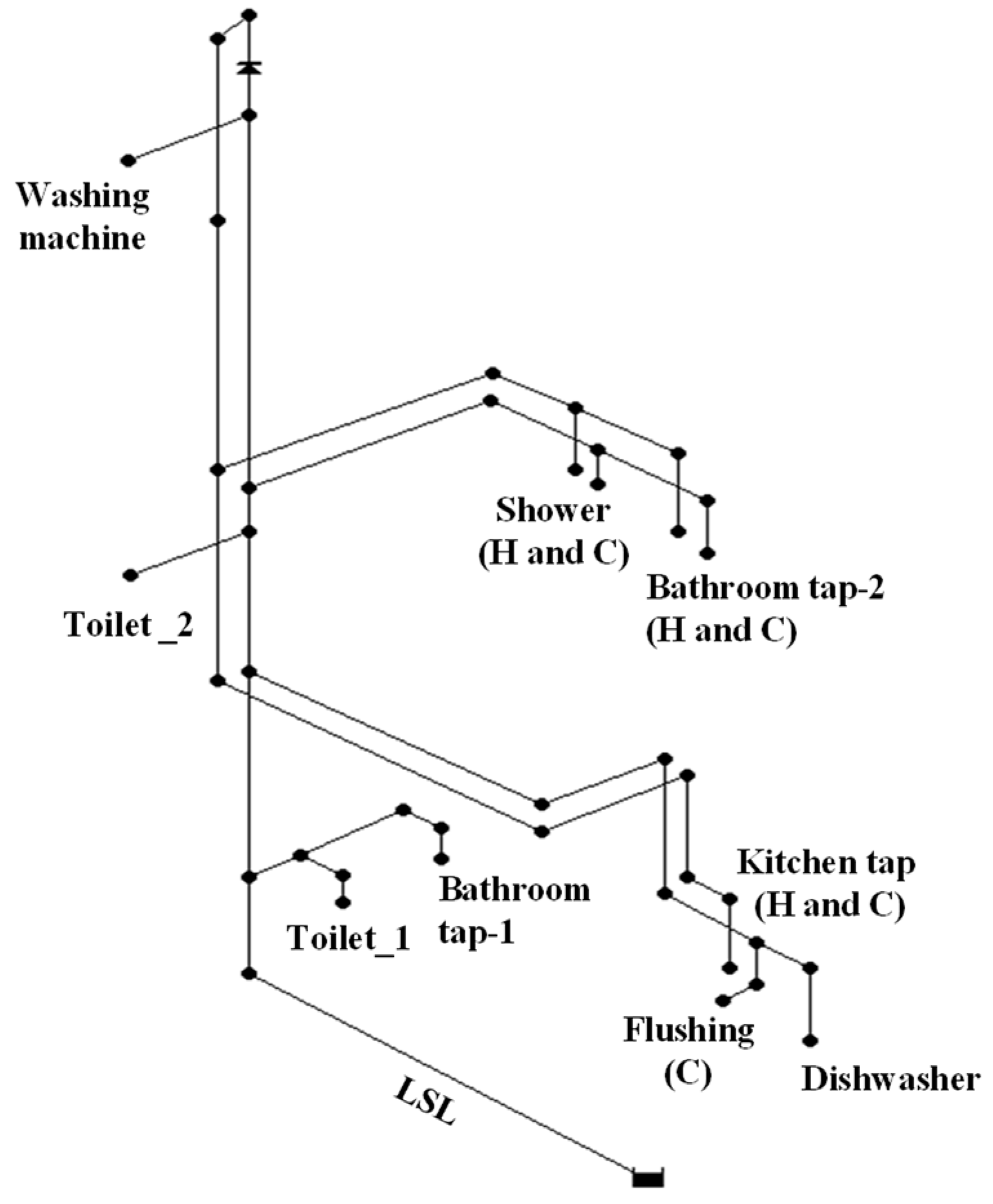
2.1. Plumbing Network Layout and Simulation Approach

Despite numerous influencing factors that determine lead levels in consumer taps during field studies, a reliable modeling approach can allow selective parameter adjustment to evaluate their impact. This study examines the combined impact of flushing and corrosion control treatments, along with diverse water consumption patterns, on spatial and temporal variations in water quality within building systems. For this investigation, a lead service line of 14 m with a diameter of 25.6 mm was introduced as the sole lead source in the plumbing system. The simulation assessed both relative water age (i.e., the duration water had spent in a household system) and dissolved lead contamination across various tap locations within a simple domestic water supply system, as shown in Figure 1. To address EPANET’s limitation of minimum time steps of one second, which can introduce inaccuracies for short pipe lengths [17], slight modifications were made to the network layout adapted from Moerman et al. [31]. Specifically, nodes with no demand were removed, reducing the number of short pipes by six. This adjustment minimized potential inaccuracies while preserving the overall network configuration.
Water consumption simulations generated using the SIMDEUM model [32] were incorporated into the EPANET (version 2.2) hydraulic and water quality network model. One week of SIMDEUM patterns per tap was generated using 10 s time steps, providing an effective way to capture the variability in consumers’ behavior. This approach captured the variability in water use throughout the day and accounted for differences between weekdays and weekends. To simulate water quality dynamics within the studied network, an extended period simulation (EPS) was conducted using EPANET over a two-week duration. This simulation period enabled the system to attain equilibrium conditions for water quality, with data from the second week used for analysis. Equilibrium was confirmed by simulating relative water age over three weeks, with fluctuations stabilizing between the second and third weeks. Lead dissolution was modeled using a first-order saturation kinetics equation, while relative water age was simulated using a zero-order reaction model. This study modeled only dissolved lead; however, particulate lead, though not included, can also contribute to higher exposure in taps. As with most EPANET-based studies, full mixing and dispersion effects were not included. Hydraulic computations were conducted with 10 s time steps, whereas water quality calculations were performed with 1 s time steps to improve temporal resolution and capture short-term variations.

2.2. Water Quality and Demand Scenarios with Flushing Strategies

This study uses two residential water demand scenarios from Hatam et al. [19] as a basis for comparison to evaluate the added impact of flushing, integrated with corrosion control measures, on lead levels under varying consumption conditions, building on a concept first presented at the 19th Computing and Control for the Water Industry Conference [33]. The total weekly average water demands are 369 lpd and 188 lpd for two inhabitants, corresponding to 184 and 94 L per capita per day (LCD) for the high-demand scenario (DH) and low-demand scenario (DL), respectively. Next to assess the impact of flushing on lead concentrations, three flushing strategies were evaluated based on both flushing volume and time. To simulate flushing demand, a node was connected to the kitchen cold-water tap via a short pipe in the model. Flushing was simulated as a one-minute event, performed either once per day (DLF0), representing 5% of total daily water use in the low-demand scenario, or three times a day (16% of total daily water use in low-demand scenario). For the three-times-per-day approach, two timing options were tested: (I) flushing every eight hours starting at midnight without aligning to usage patterns (Timing I, DLF1) or (II) flushing just before typical high-use periods during the simulated week for the kitchen tap (cold water), occurring at 6:30, 11:00, and 19:00 (Timing II, DLF2). The average weekly water demand per household for all demand scenarios and flushing strategies is summarized in Table 1. Simulations were conducted under two water quality conditions: without and with corrosion control treatment (i.e., addition of 1 mg P/L orthophosphate and pH adjustment to 7.9). The parameters for the first-order saturation kinetics equation used in the lead dissolution model were estimated based on data from a previous pilot study [34], as described in Hatam et al. [19]. Prior to modification, the water entering the pilot setup [34,35] had mean values of a pH of 7.9, alkalinity of 90 mg CaCO3/L, and DIC of 20 mg C/L at 20 °C; under the corrosion control condition, orthophosphate was added at 1 mg P/L with pH restabilization to 7.9.
The USEPA IEUBK model (version 2.0 Build 1.66) was used to estimate potential BLLs in children aged 0–84 months, based on the 90th percentile and median weekly concentrations of dissolved lead at the kitchen tap. The default IEUBK model values for input parameters, including those for soil, dust, air, diet, and drinking water intake (L/day), were used [36]. This modeling approach aligns with previous studies varying only water lead concentrations while keeping other exposure media at default levels to evaluate the impact of drinking water on BLLs. [28,29,37,38,39].

3. Results and Discussion

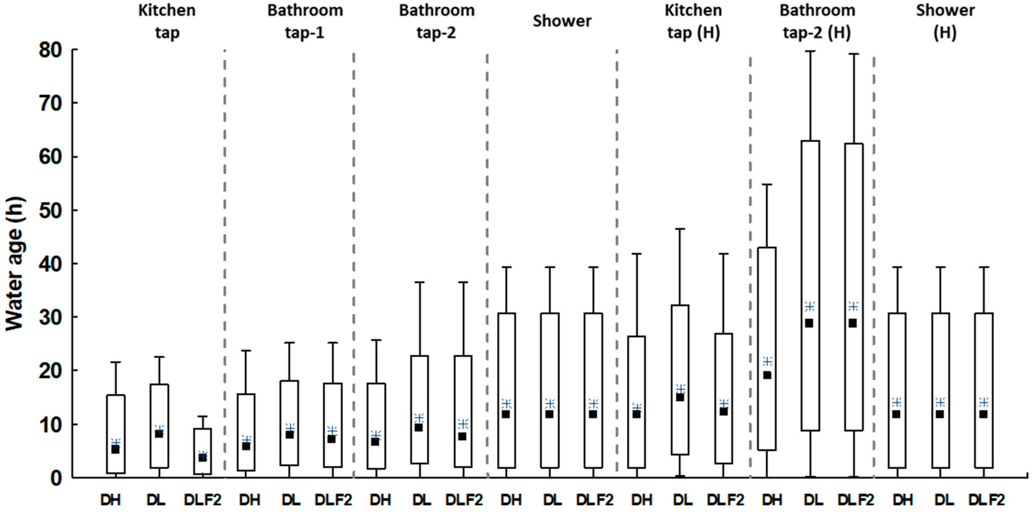
3.1. Influence of Flushing and Conservation Measures on Water Age

Figure 2 shows the distribution of relative water age across various taps over a one-week simulation, including periods of no use, comparing high- and low-demand scenarios and one of the flushing strategies (16%, Timing II). Relative water age results are illustrated over the course of one week at all times, with data being reported at 10 s intervals. The results show that the median relative water age at the kitchen tap (cold water) increased from 5 h in the high-demand to 8 h in the low-demand scenario and decreased to 3 h in the flushing scenario (DLF2) including periods of no use. The relative water age values were generally higher for the hot water, which could go up to 80 h at the bathroom tap, even without accounting the capacity of the boiler tank in the model (Figure 2). For the shower, water age was nearly identical for both hot and cold lines, which can be explained by the fact that hot and cold water are typically used simultaneously (297 L cold vs. 377 L hot over a week). In contrast, at bathroom tap-2, the usage was more uneven (22 L cold vs. 67 L hot), leading to greater differences in water age between the two lines. In the data shown in Figure 2, flushing reduced the relative water age at the kitchen tap (cold water), with minimal impact on the relative water age at other taps. This can be explained by the fact that flushing occurred near the kitchen cold tap and was timed before periods of high usage at the kitchen tap (DLF2). Furthermore, flushing reduced the variability in water ages from 22.5 to 11.5 h at the kitchen cold tap. These results are consistent with findings from Clements et al. [22], showing that purging decreased the median water age from 24.5 h to as low as 10 h for the shower (cold water), under the same building layout, with variations depending on the timing and frequency of flushing.

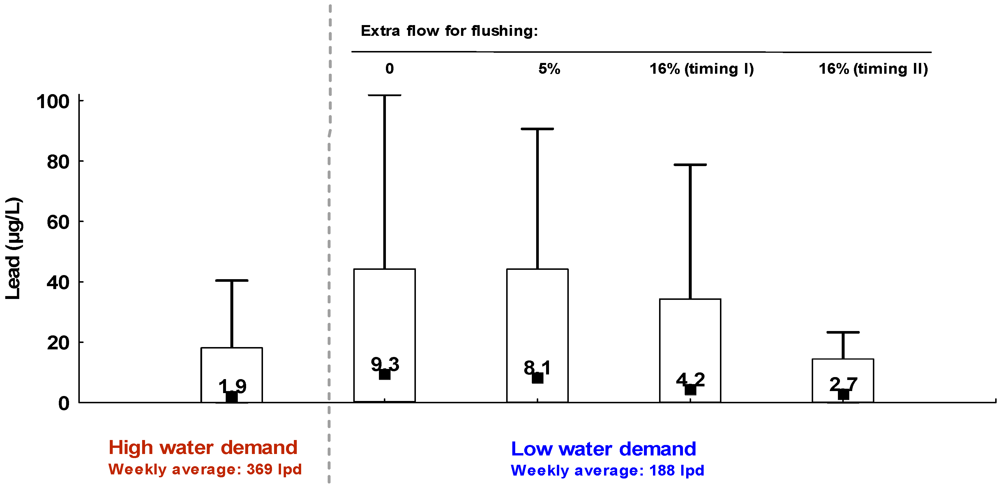
3.2. Effects of Flushing Frequency and Timing on Lead Levels

Figure 3 presents the distribution of dissolved lead concentration at the kitchen tap during usage under three flushing strategies, all applied during low-demand conditions. The high-demand scenario, based on Hatam et al. [19], is included as a reference for comparison, and all simulations were conducted without corrosion control measures. This comparison shows how different flushing strategies can reduce concentration in drinking water during periods of low water consumption. Without any flushing, the low-demand scenario resulted in median lead concentrations of 9.3 µg/L, significantly higher than the 1.9 µg/L observed under the high-demand scenario. An extra 5% of total consumption was used for flushing once a day for 1 min. In contrast, flushing three times per day (one minute per event) increased the total daily water usage by 16% in the low-demand scenario. Figure 3 illustrates that flushing every eight hours, without considering usage patterns (Timing I, DLF1), leads to higher lead levels (median 4.2 µg/L) compared to flushing before typical high-use periods (6:30, 11:00, and 19:00) at the kitchen tap with the same frequency and volume (Timing II, DLF2, median 2.7 µg/L). These findings further reinforce the emphasis by Clements et al. [22] on scheduling purging around occupancy patterns, such as before occupants wake up or return from work, to effectively minimize water age. Importantly, the range of values to which the consumer may be exposed at a given consumption time decreases by a factor of 3.4. The trend observed here with lead levels aligns with findings from Clements et al. [22] on the impact of flushing on water age, where higher purging frequency and volume resulted in lower water ages.

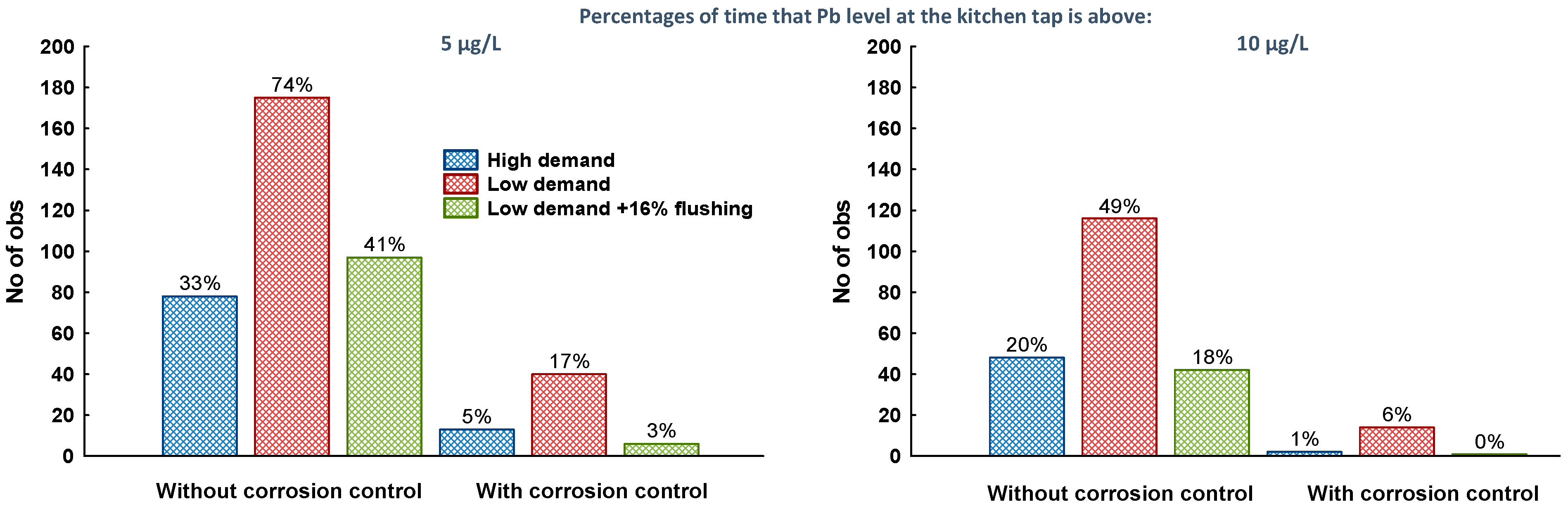
3.3. Combined Effect of Flushing and Corrosion Control Measures

Understanding the variation in and evolution of water quality standards and guidelines across countries is crucial, as these differences can influence decisions regarding recommended remedial actions. Figure 4 compares the durations of periods over a week during which lead concentrations at the kitchen tap exceeded 5 µg/L and 10 µg/L, based on simulations using 10 s interval data. Three demand and flushing scenarios were modeled, each with and without corrosion control. The occurrence of lead exceedances at the kitchen tap varied widely across different scenarios: from 74% to 3% of usage time for the 5 µg/L threshold and from 49% to 0% for the 10 µg/L threshold. In the high-demand scenario without corrosion control measures, the occurrence of lead level exceedance at the kitchen tap was 33% (>5 µg/L) and 20% of usage time (>10 µg/L). Under the lower-demand scenario, these increased sharply to 74% and 49%, respectively. However, implementing one-minute flushing three times a day (Timing II) considerably reduced exceedance to 41% (>5 µg/L) and 18% (>10 µg/L). Adding orthophosphate as a corrosion control treatment decreased the exceedances from 33% to 5% in the high- and from 74% to 17% in the low-demand scenarios. These findings indicate that, particularly under low-water-demand conditions and in the presence of LSLs, orthophosphate dosing alone (1 mg P/L) may not always be sufficient to meet the regulatory thresholds. Notably, the combined use of flushing and corrosion control measures under the low-demand scenario reduced exceedances to only 3% of usage time for the 5 µg/L threshold (an 82% reduction compared to those under corrosion control alone which were 17%), with no concentrations exceeding 10 µg/L threshold. While flushing may appear to contradict water conservation efforts, the additional water required for flushing was evaluated and should be minimized while improving water quality. In the simulated scenarios, a 16% increase in water consumption due to flushing resulted in an overall consumption of 219 lpd per household under the low-demand scenario, which was still 41% lower than that in the high-demand scenario (369 lpd). These findings suggest that a moderate increase in water use, particularly when combined with corrosion control, can yield substantial reductions in lead exposure, while maintaining overall household consumption below that of high-demand conditions.

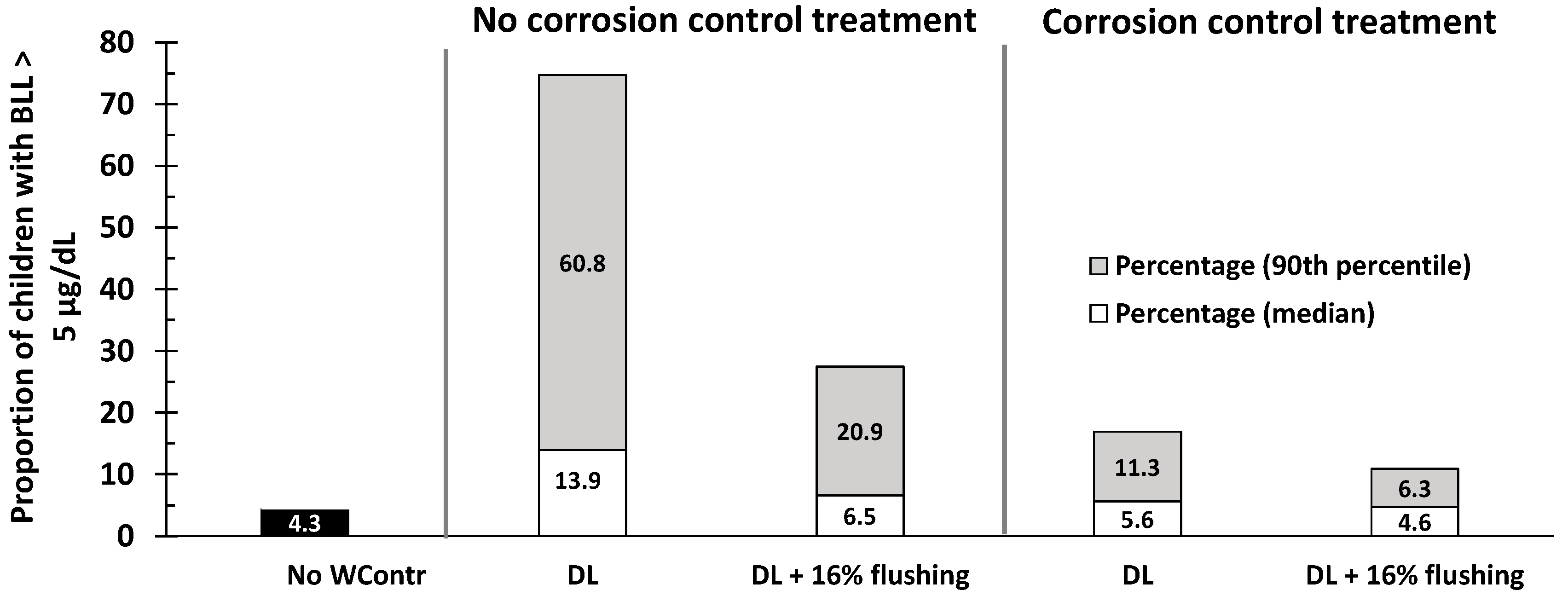
3.4. Potential Blood Lead Level Impact

The simulated lead concentrations at the kitchen tap were subsequently used as inputs for the IEUBK model to estimate the percentage of children aged 0 to 84 months with BLL exceeding 5 μg/dL. This approach enabled us to quantify how flushing may lead to potential reductions in the prevalence of elevated blood lead levels among young children. Figure 5 illustrates the effect of various mitigation strategies under low-demand conditions on the estimated percentage of children with elevated BLLs. This analysis considers both the median and the 90th percentile of lead levels at the kitchen tap during usage. When using 90th-percentile kitchen tap lead concentrations, the percentage of children exceeding the CDC’s BLL reference level of 5 μg/dL [40] increased sharply: from 4.3% with no tap water contribution to 60.8% under the low-demand scenario (DL) without any corrosion control. Under corrosion control alone, the percentage of children with elevated BLLs was 11.3%, as previously shown in Hatam et al. [19]. This outcome improved further when corrosion control was combined with a flushing program (resulting in a 16% rise in overall consumption), reducing the estimated percentage of BLL exceedances to 6.3%, based on the 90th-percentile lead levels (Figure 5). These findings show the major impact that lower water use can have on children’s lead exposure and emphasize the importance of implementing combined strategies, enhanced corrosion control treatment, and targeted flushing, especially while LSLs remain in place.

3.5. Implications for Utilities

Integrating advanced modeling techniques can improve the precision of predictions and deepen understanding of how lead behaves and migrates through water systems over time. Hydraulic models can be used to predict the impact of water-conservation strategies, water chemistry, and preventive or corrective actions on drinking water quality in both water distribution networks and buildings. These models also offer valuable insights into managing lead exposure risks in drinking water systems. When combined with stochastic demand models, hydraulic simulations can support the development of optimized regulatory sampling protocols for lead and enhance assessment of lead exposure risks; ultimately leading to more targeted and effective mitigation strategies. This study demonstrates the application of numerical tools to assess additional preventive and corrective measures for controlling lead levels in buildings with lead service lines, particularly under conditions of reduced water demand.
These results highlight the limitations of corrosion control at low orthophosphate dosages (1 mg P/L) in the presence of low demand, where exceedances (>5 µg/L) reached 17%, compared to 5% under high demand. Improved performance of corrosion control could potentially be achieved through higher orthophosphate dosing, though this would incur additional costs. A well-designed flushing strategy, which considers factors such as volume and timing, can further reduce exposure. Considering the 5 µg/L standard, the results indicate that flushing can offer greater benefits in reducing lead levels in low-consumption scenarios when combined with corrosion control. However, in the absence of corrosion control, more intensive flushing before periods of consumption may be necessary to limit exposure, albeit at the expense of increased water usage and reduced alignment with conservation goals.
Water managers should take multiple factors into account when developing effective sampling and flushing protocols. These includes the characteristics and locations of lead sources, water usage and consumption patterns, building hydraulics, and key water quality parameters. For more effective risk reduction, remedial measures can be combined with usage protocols, for example, using only water for drinking from a flushed tap, typically the kitchen tap, and avoiding water from bathroom taps. Users should also avoid filling glasses for consumption overnight to minimize potential lead exposure.
However, flushing should be viewed as short-term mitigation measures, with limited long-term efficacy and notable water wastage. As manual flushing can be tedious and may not be implemented correctly by the user, an automated flushing system installed adjacent to the kitchen tap or simply the use of an automatic flushing faucet could be considered. Even when corrosion control is implemented, it is now recognized that managers should plan to replace LSLs as it is the only long-term solution to reduce lead exposure risks in taps from LSLs [3].

3.6. Limitations and Future Work

Enhanced hydraulic and water quality modeling tools, particularly when combined with stochastic demand models such as SIMDEUM and calibrated against field data, can support future research aimed at maintaining water quality in building plumbing systems. These integrated approaches offer valuable opportunities to advance understanding of the complex effects that emerging water conservation strategies may have on water quality. Advanced modeling techniques can also enable the simultaneous consideration of multiple interacting factors, including increased stagnation, biofilm formation, disinfectant depletion, lead leaching from lead sources, proliferation of opportunistic pathogens, and temperature variations.
While modeling serves as a valuable tool for managing building water systems to estimate true exposure to reduce public health risks, further research is needed to more accurately simulate real-world phenomena such as dispersion and mixing dynamics. These aspects were not accounted in the current study and require further investigation to enhance predictive accuracy and inform effective mitigation strategies. Particulate lead, though not considered in this model, can also contribute to significant exposure at the tap. The release of particulate lead is highly site-specific, reflecting hydraulics, use patterns, and materials, and interestingly flushing has been shown to decrease exposure to particulate in some systems [34,38]. Abokifa and Biswas [41] simulated the release of both particulate and dissolved lead under normal household usage. However, modeling the detachment and transport of particulate lead is challenging and simplified models fail to capture the truly random nature of particulate lead and further investigation is recommended for better simulating the random nature of particulate lead release [16].
Moreover, the modeling approach here could be extended to a broader range of water quality parameters and building topologies with varying occupancy patterns. This study focused specifically on decreased flow intensity as a representation of water conservation, without incorporating variability in usage duration. Future research should also involve assessing the effectiveness of flushing in reducing lead contamination from other internal sources like leaded brass, solders, or distal plumbing components, an area that could benefit from the methodology presented in this study. Finally, future work should explore the implications of temperature changes caused by climate changes or seasonal variations as these can drastically increase lead release from LSLs.

4. Conclusions

Despite the complexity of real-world conditions influencing lead levels at consumer taps, this study shows that a modeling approach can enable targeted adjustment of key parameters, offering valuable insights into their individual and combined effects. This modeling-based evaluation contributes to a better understanding of short-term lead control strategies in water-conserving households and their potential health implications, particularly where immediate LSL replacement is not feasible. First, flushing significantly reduced the relative water age at the kitchen tap (cold water) under low-demand conditions, from 8 to 3 h including periods of no use, while having minimal effect on other taps. Under the studied water conservation scenario, the results indicate that a combination of corrosion control treatment and a targeted flushing plan as a short-term action can significantly lower lead levels. In low-water-consumption conditions, flushing alone reduced exceedances from 74% to 41% (>5 µg/L), while orthophosphate alone brought them down to 17%. Combined, these measures lowered exceedances to only 3% (>5 µg/L) of usage time and eliminated exceedances above 10 µg/L threshold. Although increasing water use through flushing may conflict with water conservation goals, a modest 16% rise over the low-demand scenario resulted in an 82% reduction in lead exceedances compared to corrosion control alone. Despite this increase, total household consumption remained 41% lower than that in high-demand scenarios, suggesting that the combined approach may serve as a viable short-term mitigation strategy in low-consumption settings. Furthermore, under low-demand conditions, the combined targeted flushing and corrosion control strategy reduced the predicted percentage of children aged 0–84 months with BLLs exceeding 5 μg/dL from 61% to 6%, based on IEUBK model estimates using 90th percentile of lead concentrations at the kitchen tap. This modeling-based evaluation contributes to a better understanding of short-term lead control strategies in water-conserving households and their potential health implications. It can apply to any water quality type and materials with known reaction rates, allowing the assessment of the impact of varying demand and occupation patterns across different building layouts and the evaluation of the effectiveness of preventative interventions.

Author Contributions

Conceptualization, F.H., M.B. and M.P.; Methodology, F.H., M.B. and M.P.; Software, F.H. and M.B.; Investigation, F.H. and M.P.; Writing—original draft, F.H.; Writing—review & editing, M.B. and M.P. All authors have read and agreed to the published version of the manuscript.

Funding

This research was funded by the Industrial Chair on Drinking Water at Polytechnique Montréal grant number NSERC-ALLRP 560764–20.

Data Availability Statement

The data presented in this study are available on request from the corresponding author.

Acknowledgments

The authors acknowledge the financial support provided by the Industrial Chair on Drinking Water at Polytechnique Montréal, which is funded by NSERC and its industrial partners: the City of Montréal, Veolia Water Technologies Canada, the City of Laval, the City of Longueuil, the City of Repentigny, the City of Joliette, and the City of L’Assomption.

Conflicts of Interest

The authors declare no conflict of interest.

References

  1. Health Canada. Guidelines for Canadian Drinking Water Quality Guideline Technical Document. Lead; Government of Canada: Ottawa, ON, Canada, 2019; p. 113. [Google Scholar]
  2. Health Canada; Federal-Provincial-Territorial Committee on Drinking Water. Lead in Drinking Water; Health Canada: Ottawa, ON, Canada, 2017; p. 107. [Google Scholar]
  3. United States Environmental Protection Agency (USEPA). National Primary Drinking Water Regulations: Lead and Copper Rule Revisions, 2021; Federal Register: Washington, DC, USA, 2021; Volume 86.
  4. World Health Organization (WHO). Childhood Lead Poisoning; World Health Organization: Geneva, Switzerland, 2010; p. 74. [Google Scholar]
  5. Lanphear, B.P.; Hornung, R.; Khoury, J.; Yolton, K.; Baghurst, P.; Bellinger, D.C.; Canfield, R.L.; Dietrich, K.N.; Bornschein, R.; Greene, T.; et al. Low-level environmental lead exposure and children’s intellectual function: An international pooled analysis. Environ. Health Perspect. 2005, 113, 894–899. [Google Scholar] [CrossRef] [PubMed]
  6. Dettori, M.; Arghittu, A.; Deiana, G.; Castiglia, P.; Azara, A. The revised European Directive 2020/2184 on the quality of water intended for human consumption. A step forward in risk assessment, consumer safety and informative communication. Environ. Res. 2022, 209, 112773. [Google Scholar] [CrossRef]
  7. Elfland, C.; Scardina, P.; Edwards, M. Lead-contaminated water from brass plumbing devices in new buildings. J. Am. Water Work Assoc. 2010, 102, 66–76. [Google Scholar] [CrossRef]
  8. UNESCO; UN-Water. Water and Climate Change; UNESCO: Paris, France, 2020. [Google Scholar]
  9. Ministère du Développement durable, de l’Environnement et de la Lutte contre les changements climatiques (MDDELCC). 2018–2030 Québec Water Strategy; Communications Branch of MDDELCC: Québec, QC, Canada, 2018.
  10. United States Environmental Protection Agency (USEPA). WaterSence at Work. Best Management Practices for Commercial and Institutional Facilities; EPA 832-F-12-034; EPA WaterSence: Washington, DC, USA, 2012; p. 308.
  11. Proctor, C.; Rhoads, W.J.; Keane, T.; Salehi, M.; Hamilton, K.; Pieper, K.J.; Cwiertny, D.M.; Prévost, M.; Whelton, A. Considerations for large building water quality after extended stagnation. AWWA Water Sci. 2020, 2, e1186. [Google Scholar] [CrossRef]
  12. Salehi, M.; Odimayomi, T.; Ra, K.; Ley, C.; Julien, R.; Nejadhashemi, A.P.; Hernandez-Suarez, J.S.; Mitchell, J.; Shah, A.D.; Whelton, A. An investigation of spatial and temporal drinking water quality variation in green residential plumbing (sumbitted). Build. Environ. 2020, 169, 106566. [Google Scholar] [CrossRef]
  13. Hatam, F.; Ebacher, G.; Prévost, M. Stringency of water conservation determines drinking water quality trade-offs: Lessons learned from a full-scale water distribution system. Water 2021, 13, 2579. [Google Scholar] [CrossRef]
  14. Agudelo-Vera, C.; Blokker, M.; Vreeburg, J.; Vogelaar, H.; Hillegers, S.; van der Hoek Jan, P. Testing the robustness of two water distribution system layouts under changing drinking water demand. J. Water Resour. Plann. Manag. 2016, 142, 05016003. [Google Scholar] [CrossRef]
  15. Zhuang, J.; Sela, L. Impact of emerging water savings scenarios on performance of urban water networks. J. Water Resour. Plann. Manag. 2020, 146, 04019063. [Google Scholar] [CrossRef]
  16. Burkhardt, J.B.; Woo, H.; Mason, J.; Shang, F.; Triantafyllidou, S.; Schock Michael, R.; Lytle, D.; Murray, R. Framework for modeling lead in premise plumbing systems using EPANET. J. Water Resour. Plann. Manag. 2020, 146, 04020094. [Google Scholar] [CrossRef]
  17. Dash, A.; van Steen, J.; Blokker, M. Robustness of Profile Sampling in Detecting Dissolved Lead in Houshold Drinking Water. In Proceedings of the 2nd International Joint Conference on Water Distribution Systems Analysis & Computing and Control in the Water Industry, Valencia, Spain, 18–22 July 2022. [Google Scholar]
  18. Maheshwari, A.; Abokifa, A.A.; Biswas, P.; Gudi, R.D. Framework for evaluating the impact of water chemistry changes in full-scale drinking water distribution networks on lead concentrations at the tap. J. Environ. Eng. 2020, 146, 04020051. [Google Scholar] [CrossRef]
  19. Hatam, F.; Blokker, M.; Doré, E.; Prévost, M. Reduction in water consumption in premise plumbing systems: Impacts on lead concentration under different water qualities. Sci. Total Environ. 2023, 879, 162975. [Google Scholar] [CrossRef] [PubMed]
  20. Vizanko, B.; Kadinski, L.; Ostfeld, A.; Berglund, E.Z. Social distancing, water demand changes, and quality of drinking water during the COVID-19 pandemic. Sustain. Cities Soc. 2024, 102, 105210. [Google Scholar] [CrossRef]
  21. Burkhardt, J.B.; Minor, J.; Platten, W.E.; Shang, F.; Murray, R. Relative water age in premise plumbing systems using an agent-based modeling framework. J. Water Resour. Plann. Manag. 2023, 149, 04023007. [Google Scholar] [CrossRef] [PubMed]
  22. Clements, E.; Irwin, C.; Taflanidis, A.; Bibby, K.; Nerenberg, R. Impact of fixture purging on water age and excess water usage, considering stochastic water demands. Water Res. 2023, 245, 120643. [Google Scholar] [CrossRef]
  23. Lanphear, B.P.; Rauch, S.; Auinger, P.; Allen, R.W.; Hornung, R.W. Low-level lead exposure and mortality in US adults: A population-based cohort study. Lancet Public Health 2018, 3, e177–e184. [Google Scholar] [CrossRef]
  24. Lustberg, M.; Silbergeld, E. Blood lead levels and mortality. Arch. Intern. Med. 2002, 162, 2443–2449. [Google Scholar] [CrossRef] [PubMed]
  25. Ziegler, E.E.; Edwards, B.B.; Jensen, R.L.; Mahaffey, K.R.; Fomon, S.J. Absorption and retention of lead by infants. Pediatr. Res. 1978, 12, 29–34. [Google Scholar] [CrossRef]
  26. Manton, W.I.; Angle, C.R.; Stanek, K.L.; Reese, Y.R.; Kuehnemann, T.J. Acquisition and retention of lead by young children. Environ. Res. 2000, 82, 60–80. [Google Scholar] [CrossRef]
  27. Levallois, P.; St-Laurent, J.; Gauvin, D.; Courteau, M.; Prévost, M.; Campagna, C.; Lemieux, F.; Nour, S.; D’Amour, M.; Rasmussen, P.E. The impact of drinking water, indoor dust and paint on blood lead levels of children aged 1–5 years in Montreal (Québec, Canada). J. Expo. Sci. Environ. Epidemiol. 2013, 24, 185–191. [Google Scholar] [CrossRef]
  28. Deshommes, E.; Prévost, M.; Levallois, P.; Lemieux, F.; Nour, S. Application of lead monitoring results to predict 0–7 year old children’s exposure at the tap. Water Res. 2013, 7, 2409–2420. [Google Scholar] [CrossRef]
  29. Ngueta, G.; Prévost, M.; Deshommes, E.; Abdous, B.; Gauvin, D.; Levallois, P. Exposure of young children to household water lead in the Montreal area (Canada): The potential influence of winter-to-summer changes in water lead levels on children’s Blood lead concentration. Environ. Int. 2014, 73, 57–65. [Google Scholar] [CrossRef]
  30. Stanek, L.W.; Xue, J.; Lay, C.R.; Helm, E.C.; Schock, M.; Lytle, D.A.; Speth, T.F.; Zartarian, V.G. Modeled impacts of drinking water Pb reduction scenarios on children’s exposures and blood lead levels. Environ. Sci. Technol. 2020, 54, 9474–9482. [Google Scholar] [CrossRef]
  31. Moerman, A.; Blokker, M.; Vreeburg, J.; van der Hoek, J.P. Drinking Water Temperature Modelling in Domestic Systems. In Proceedings of the 16th Water Distribution System Analysis Conference, WDSA2014, Bari, Italy, 14–17 July 2014; pp. 143–150. [Google Scholar]
  32. Blokker, E.J.M.; Vreeburg, J.H.G.; van Dijk, J.C. Simulating residential water demand with a stochastic end-use model. J. Water Resour. Plan. Manag. ASCE 2010, 136, 19–26. [Google Scholar] [CrossRef]
  33. Hatam, F.; Blokker, E.; Prévost, M. Evaluation of flushing and corrosion control to lower lead levels at the taps in households with lead service lines. In Proceedings of the 19th Computing and Control for the Water Industry Conference (CCWI), Leicester, UK, 4–7 September 2023. [Google Scholar]
  34. Doré, E.; Deshommes, E.; Laroche, L.; Nour, S.; Prévost, M. Lead and copper release from full and partially replaced harvested lead service lines: Impact of stagnation time prior to sampling and water quality. Water Res. 2019, 150, 380–391. [Google Scholar] [CrossRef] [PubMed]
  35. Doré, E.; Deshommes, E.; Laroche, L.; Nour, S.; Prévost, M. Study of the long-term impacts of treatments on lead release from full and partially replaced harvested lead service lines. Water Res. 2019, 149, 566–577. [Google Scholar] [CrossRef]
  36. United States Environmental Protection Agency (USEPA). User’s Guide for the Integrated Exposure Uptake Biokinetic Model for Lead in Children (IEUBK); Version 2.0; United States Environmental Protection Agency: Washington, DC, USA, 2021.
  37. Deshommes, E.; Andrews, R.C.; Gagnon, G.; McCluskey, T.; McIlwain, B.; Dore, E.; Nour, S.; Prevost, M. Evaluation of exposure to lead from drinking water in large buildings. Water Res. 2016, 99, 46–55. [Google Scholar] [CrossRef]
  38. Doré, E.; Deshommes, E.; Andrews, R.C.; Nour, S.; Prévost, M. Sampling in schools and large institutional buildings: Implications for regulations, exposure and management of lead and copper. Water Res. 2018, 140, 110–122. [Google Scholar] [CrossRef]
  39. Keeley, S.; Dorevitch, S.; Kelly, W.; Jacobs, D.E.; Geiger, S.D. IEUBK Modeling of Children’s Blood Lead Levels in Homes Served by Private Domestic Wells in Three Illinois Counties. Int. J. Environ. Res. Public Health 2024, 21, 337. [Google Scholar] [CrossRef] [PubMed]
  40. Centers for Disease Control and Prevention (CDC). Response to Advisory Committee on Childhood Lead Poisoning Prevention Recommendations in “Low Level Lead Exposure Harms Children: A Renewed Call of Primary Prevention”; Centers for Disease Control and Prevention: Atlanta, GA, USA, 2012.
  41. Abokifa, A.A.; Biswas, P. Modeling soluble and particulate lead release into drinking water from full and partially replaced lead service lines. Environ. Sci. Technol. 2017, 51, 3318–3326. [Google Scholar] [CrossRef]
Figure 1. The network layout is derived from Moerman et al. (2014) [31] with minor adjustments. The network includes several taps. The labels ‘H’ and ‘C’ indicate hot and cold water, respectively. A node is linked to the cold kitchen tap via a short pipe for modeling flushing demand.
Water 17 02297 g001
Figure 2. Distribution of relative water age at various taps over an entire week under high demand (DH), low demand (DL), and low demand with flushing (DLF2; 16%, Timing II), including periods of no use. Square: median; star: mean; box: 10–90%; whisker: min-max.
Water 17 02297 g002
Figure 3. Distribution of simulated dissolved lead concentrations at kitchen tap (cold water) during usage, without any corrosion control, under high- and low-water-demand scenarios. For the low-demand scenario, three flushing strategies were tested: once daily (5% of use in low-demand scenario) and three times daily (16%) using two different timing schemes (Timing I and II). Square: median lead concentration; box: 10–90%; whisker: non-outlier range.
Water 17 02297 g003
Figure 4. Percentage of time lead levels at the kitchen tap exceed 5 and 10 µg/L during usage time (based on a 10 s reporting interval). Scenarios include high demand, low demand, and low demand with one minute flushing three times daily (Timing II), each modeled with and without corrosion control.
Water 17 02297 g004
Figure 5. Proportion of children with blood lead levels (BLLs) >5 μg/dL under the low-demand scenario, showing the impact of flushing (16%, Timing II) and corrosion control. Results are shown using both the median and 90th percentile of lead levels at the kitchen tap during usage. No WContr = no tap water contribution; DL = low-demand scenario.
Water 17 02297 g005
Table 1. Summary of total average weekly water demand per household for all the demand scenarios and flushing strategies, with percentage increase relative to DL.
ScenariosAverage Weekly Demand Per Household (lpd)% of Increase
High demand (DH)368.996
Low demand (DL)188.30
Flushing once a day (DLF0)198.55
Flushing three times a day (DLF1), (Timing I)218.616
Flushing three times a day (DLF2), (Timing II)218.616
Disclaimer/Publisher’s Note: The statements, opinions and data contained in all publications are solely those of the individual author(s) and contributor(s) and not of MDPI and/or the editor(s). MDPI and/or the editor(s) disclaim responsibility for any injury to people or property resulting from any ideas, methods, instructions or products referred to in the content.

