Research on Startup Characteristics of Parallel Axial-Flow Pump Systems

Abstract

This study takes four parallel axial-flow pumps (three in operation + one on standby) as the research object. Using a 1D–3D coupling method, it explores the flow characteristics of axial-flow pumps under different startup strategies during multi-pump parallel operation. Through comparative analysis, the following conclusions are drawn: when all three pumps start simultaneously, the internal pressure exceeds the rated head by 23.43%, and the reverse flow reaches 10.57% of the rated flow. When starting the pumps sequentially with 5 s intervals, the pressure can be reduced to 11.41% above the rated head, but the reverse flow increases to 13.87%. Further extending the startup interval to 15 s results in only minimal improvements compared to 5 s intervals: the maximum internal pressure and maximum reverse flow decrease by just 0.97% and 0.05%, respectively. When valve coordination is added to the 5 s sequential startup strategy (pre-opening the valve to 60% before pump startup), the pressure exceeds the rated head by 10.49%, and the reverse flow exceeds the rated flow by 6.04%. In this scenario, the high-pressure areas and high-turbulence zones on the blade back surfaces are significantly reduced, achieving optimal flow stability. Therefore, the parallel system startup should adopt a coordinated strategy combining moderate time intervals with 60% valve pre-opening. This approach can both avoid excessive pressure impact and effectively control reverse flow phenomena, providing an important basis for optimizing the startup of multi-pump parallel systems.

1. Introduction

In China, large-capacity pumping stations employ diverse pump types, including axial-flow, mixed-flow, tubular-flow, and centrifugal pumps. Among these, vertical axial-flow pumps have gained predominant adoption due to their space-saving design, low-lift operation, high discharge capacity, operational stability, and convenient installation/maintenance features [1]. These pumping systems play a critical role in national infrastructure, serving vital functions in flood control, agricultural water management, field drainage, and inter-basin water diversion projects [2]. The transient startup phase of axial-flow pumps involves significant variations in operational parameters such as rotational speed, hydraulic head, and flow rate [3]. The starting methodology employed substantially influences system safety, operational stability, and energy efficiency. Different startup techniques demonstrate distinct characteristics in terms of dynamic response, power consumption, and mechanical stress distribution. Comprehensive investigation of various startup approaches facilitates process optimization, minimizes hydraulic and mechanical impacts on pumping systems, enhances equipment durability, and improves overall operational performance.

When the flow rate of a single axial-flow pump cannot meet user requirements, two or more pumps can be operated in parallel to increase the flow rate and satisfy actual demand. Parallel operation not only achieves a significantly higher flow rate but also serves as an effective regulation method. In parallel-operated pump units, the inlet and outlet pressures of the pumps are equal, while the total flow rate is the sum of the flow rates of each individual pump. Recent years have witnessed significant advancements in parallel pump-system research across multiple domains, including performance evaluation, control optimization, dynamic characteristic analysis, structural innovation, and renewable-energy applications. In the field of performance assessment and testing methodologies, Meng et al. [4] innovatively proposed a cost-effective yet high-precision testing and evaluation approach for large-scale vacuum pump parallel systems, which enables an accurate assessment of the pumping performance in multi-pump parallel configurations. Cui et al. [5] conducted an in-depth analysis of a multi-pump parallel system in a pumping station, investigating its output characteristics and pump selection methodology, while proposing targeted retrofit solutions to optimize the parallel system configuration and design. In the domain of control strategies and operational optimization, Xingcheng Gan et al. [6] innovatively enhanced the control scheme for a quadruple-pump parallel system through the integration of machine learning models with improved swarm intelligence algorithms. Concurrently, Zhao et al. [7] focused on variable-frequency water supply systems with parallel pumps, significantly improving the reliability of constant-pressure parallel pump units by implementing reliability zoning and optimized pump sequencing logic. Wei Cong et al. [8] developed a water resources optimization model for parallel reservoir-pump station irrigation systems and proposed a multilevel decomposition-aggregation dynamic programming (MDADP) algorithm. Subsequently, Hou Shuai et al. [9] introduced an enhanced mayfly algorithm to optimize the operation of parallel chilled water pumps, while Wang Gang et al. [10] established a comprehensive energy model based on similarity laws and Kirchhoff’s principles to improve parallel pump system efficiency. In parallel, Guo Tuanhui et al. [11] conducted fundamental research on large aircraft multi-pump hydraulic systems, developing a theoretical model that systematically accounts for pressure, flow rate, and temperature effects to analyze casing return flow interference phenomena. Abdol Mahdi Behroozi et al. [12] employed a MacCormack-based second-order time-marching finite difference scheme to discretize and solve the governing equations, investigating transient behaviors and water hammer phenomena induced by operational changes in parallel pump units. Complementing this work, Zhida Yang et al. [13] combined dynamic mesh technology with fundamental fluid dynamics to elucidate the inherent damping mechanism of check valves during reverse flow conditions and their water hammer suppression capabilities. Concurrently, Özkayar Gürhan et al. [14] developed a multiphase rectification method to mitigate flow fluctuations under low-flow conditions, subsequently deriving an analytical equation to quantify the influence of parallel pump quantity on fluid pulsation factors. In the domain of innovative pump design and applications, Ding Tian et al. [15] proposed a novel pump architecture capable of high-flow operation across multiple working conditions, featuring configurable series/parallel operation modes with demonstrated performance enhancement through optimization. Within renewable energy-driven systems, Carricondo Antón J.M. et al. [16] systematically investigated the impact of parallel pump quantity on both water delivery capacity and photovoltaic array sizing under solar power generation constraints, while Gasque María et al. [17] developed an advanced power allocation strategy that significantly improved the energy conversion efficiency (by 12–15% in field tests) and the overall utilization rate of photovoltaic pumping systems. Oh Heekyong et al. [18] implemented a real-time thermodynamic monitoring system incorporating intelligent temperature/pressure sensors, low-power wireless data communication modules, and advanced pump data analytics algorithms. In parallel developments, Baranidharan Manickavel et al. [19] pioneered a multi-parallel pump combined variable-speed technology for pumping stations, with comprehensive system validation conducted through Matlab Simulink R2025a simulations of the multi-pump drive system.

Regarding axial-flow pumps, Wang Yuxin [20] et al. conducted numerical simulations using CFD technology for five different operational configurations of a pumping station equipped with five axial-flow pumps, concluding that the designed head difference between parallel-operating pumps should not be excessively large in engineering applications. Building upon iterative methods for solving pump unit operating parameters, Zhou Longcai [21] subsequently established a dynamic programming model to determine the optimal startup combination for multiple parallel pump units.

Parallel pump operation is widely implemented in pumping stations, and existing studies have comprehensively investigated critical technical aspects including performance testing, control algorithms, dynamic characteristics, structural design, and renewable energy applications from multiple perspectives, providing substantial theoretical and technical support for parallel pump system design and optimization across industrial, aeronautical, and hydraulic engineering domains. However, current research on axial-flow pump parallel systems predominantly focuses on unit selection and system optimization, with limited investigation into transient processes during parallel pump startup—a significant knowledge gap given that improper pump–valve coordination in practical applications can induce water hammer effects and pressure pulsations that compromise system safety. Addressing this research void, the present study employs a 1D–3D coupling methodology to simulate and optimize pump–valve coordination strategies during the parallel startup of multiple axial-flow pump units, thereby enhancing the safety and stability of pumping systems during initialization.

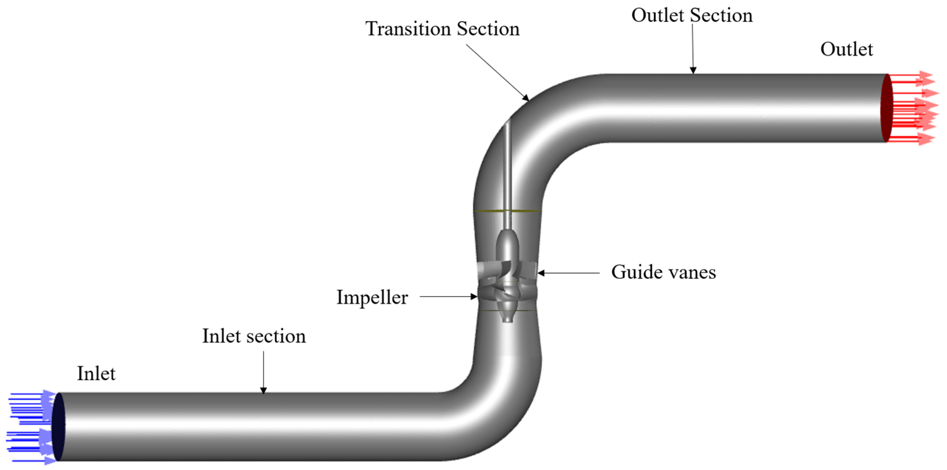
2. Physical Model and Numerical Methods

2.1. Model Parameters

The three-dimensional fluid domain of the vertical axial-flow pump was modeled using Cero 8.0 software. The model domain consists of four parts: the inlet section, impeller, guide vane, and outlet section. The main parameters are shown in

Table 1. Main parameters of the axial pump.

Parameter Name	Symbols	Values
Impeller outer diameter	D2 (mm)	350
Impeller blades	Zimp	4
GV blades	Zgui	9
Rotation speed	n (rpm)	750
Flow rate	Q (m3/s)	2.46
Head	H (m)	10.2

, the three-dimensional fluid domain model is shown in Figure 1, and the parallel system schematic of the axial-flow pump is shown in Figure 2.

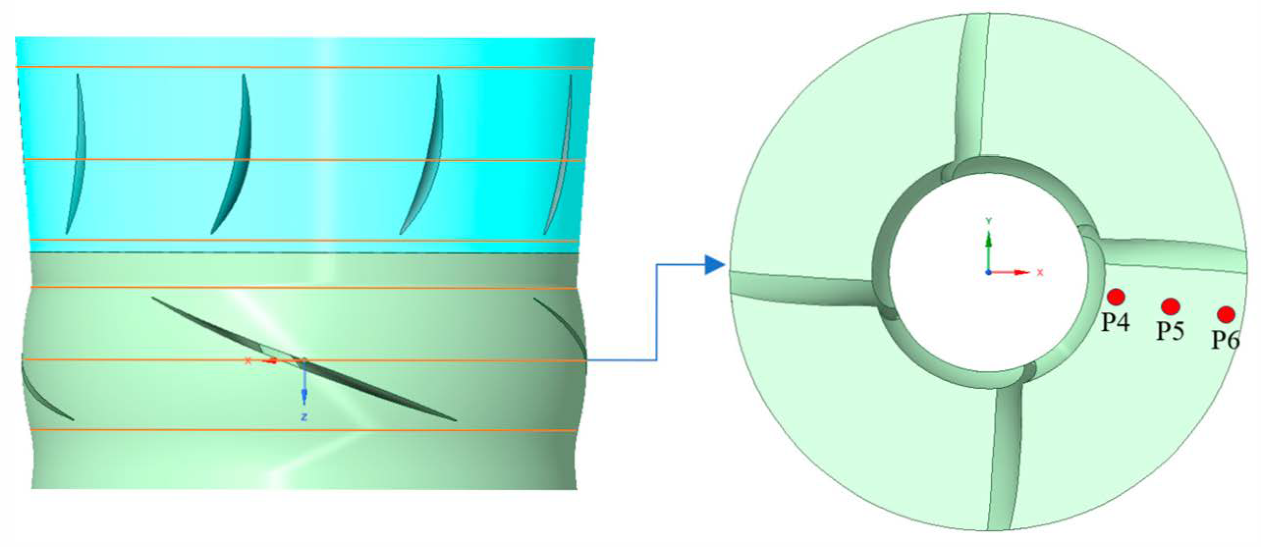
2.2. Mesh Generation

The numerical simulation accuracy was ensured through polyhedral meshing of the axial-flow pump’s fluid domain using ANSYS 19.2 Fluent Meshing. Particular attention was given to boundary layer refinement on both the impeller blade and diffuser vane surfaces. Figure 3 illustrates the computational grid distribution for key pump components.

A comprehensive mesh independence study was conducted, evaluating seven distinct grid resolutions. As shown in Figure 4, the head variation became negligible when the total cell count reached 2,846,130, which was consequently selected as the optimal mesh size for subsequent simulations.

2.3. Numerical Computation Methods and Boundary Conditions

2.3.1. Numerical Computation Methods

The internal flow dynamics in axial-flow pumps are characterized by turbulent flow regimes. The governing equations for numerical flow-field analysis are derived from the fundamental conservation laws of mass, momentum, and energy. In the present study, the working fluid is treated as incompressible (ambient-temperature clean water), reducing the governing equation system to the continuity and momentum equations.

To achieve mathematical closure of the turbulence modeling, the RNG k-ε two-equation turbulence model was employed. This model utilizes renormalization group theory to reformulate the Navier–Stokes equations, incorporating modifications to turbulent viscosity. The enhanced formulation enables accurate prediction of complex turbulent diffusion phenomena, particularly in flows exhibiting strong rotational effects, significant curvature, and high strain rates. The governing equations are expressed as follows:

Mass Conservation Equation:

$${\displaystyle \frac{\mathsf{\partial }\rho }{\mathsf{\partial }t}}+{\displaystyle \frac{\mathsf{\partial }(\rho u_i)}{\mathsf{\partial }{x}_i}}=0$$

(1)

Momentum Conservation Equation:

$${\displaystyle \frac{\mathsf{\partial }(\rho u)}{\mathsf{\partial }t}}+div(\rho uu)=div(ugrad u)-{\displaystyle \frac{\mathsf{\partial }\rho }{\mathsf{\partial }x}}$$

(2)

$${\displaystyle \frac{\mathsf{\partial }(\rho v)}{\mathsf{\partial }t}}+div(\rho vu)=div(ugrad v)-{\displaystyle \frac{\mathsf{\partial }\rho }{\mathsf{\partial }x}}$$

(3)

$${\displaystyle \frac{\mathsf{\partial }(\rho w)}{\mathsf{\partial }t}}+div(\rho wv)=div(ugrad w)-{\displaystyle \frac{\mathsf{\partial }\rho }{\mathsf{\partial }x}}$$

(4)

Turbulent Kinetic Energy (k) Equation:

$${\displaystyle \frac{\mathsf{\partial }(\rho k)}{\mathsf{\partial }t}}+{\displaystyle \frac{\mathsf{\partial }(\rho k{u}_i)}{\mathsf{\partial }{x}_i}}={\displaystyle \frac{\mathsf{\partial }}{\mathsf{\partial }{x}_j}}\left({\alpha }_k{\mu }_{eff}{\displaystyle \frac{\mathsf{\partial }k}{\mathsf{\partial }{x}_j}}\right)+G_k+\rho \epsilon$$

(5)

Turbulent Kinetic Energy Dissipation Rate (ε) Equation:

$${\displaystyle \frac{\mathsf{\partial }(\rho \epsilon )}{\mathsf{\partial }t}}+{\displaystyle \frac{\mathsf{\partial }(\rho \epsilon u_i)}{\mathsf{\partial }{x}_i}}={\displaystyle \frac{\mathsf{\partial }}{\mathsf{\partial }{x}_j}}\left({\alpha }_{\epsilon }{\mu }_{eff}{\displaystyle \frac{\mathsf{\partial }\epsilon }{\mathsf{\partial }{x}_j}}\right)+{C_{1\epsilon }}^{*}{\displaystyle \frac{\epsilon }{k}}{G}_k-C_{2\epsilon }\rho {\displaystyle \frac{{\epsilon }^2}{k}}$$

(6)

In the equation, $G_k$ can be expressed as $G_k={\mu }_t\left({\displaystyle \frac{\mathsf{\partial }{u}_i}{\mathsf{\partial }{x}_j}}+{\displaystyle \frac{\mathsf{\partial }{u}_j}{\mathsf{\partial }{x}_i}}\right){\displaystyle \frac{\mathsf{\partial }{u}_i}{\mathsf{\partial }{x}_j}}$; ${\mu }_{eff}=\mu +{\mu }_t$; ${\mu }_t={\displaystyle \frac{\rho C_{\mu }{k}^2}{\epsilon }}$, which represents the generation term of turbulent kinetic energy k; $C_{\mu }=0.0845$; α_ε and α_k are the Prandtl numbers associated with dissipation rate ε and turbulent kinetic energy k, respectively. ${\alpha }_k=1.39$, ${\alpha }_{\epsilon }=1.39$; ${C_{1\epsilon }}^{*}=C_{1\epsilon }-{\displaystyle \frac{\eta (1-\frac{\eta }{{\eta }_0})}{1+\beta {\eta }^3}}$. Empirical constants: $C_{1\xi }=1.42$, $C_{2\xi }=1.68$; $\eta ={\left(2E_{ij}\times E_{ij}\right)}^{{\displaystyle \frac{1}{2}}}{\displaystyle \frac{k}{\epsilon }}$, $E_{ij}={\displaystyle \frac{1}{2}}\left({\displaystyle \frac{\mathsf{\partial }{u}_i}{\mathsf{\partial }{x}_j}}+{\displaystyle \frac{\mathsf{\partial }{u}_j}{\mathsf{\partial }{x}_i}}\right)$, ${\eta }_0=4.377$, $\beta =0.012$.

2.3.2. Method of Characteristics

The one-dimensional equations can be divided into the continuity equation and the momentum equation. These equations comprehensively reflect the variation patterns of transient flow in pipelines and represent one form of expression for one-dimensional wave equations. Through discretization and derivation, these equations can be expressed as a system of two partial differential equations [22].

$$g{\displaystyle \frac{\mathsf{\partial }H}{\mathsf{\partial }x}}+V{\displaystyle \frac{\mathsf{\partial }V}{\mathsf{\partial }x}}+{\displaystyle \frac{\mathsf{\partial }V}{\mathsf{\partial }t}}+{\displaystyle \frac{fV\left|V\right|}{2D}}=0$$

(7)

$$V{\displaystyle \frac{\mathsf{\partial }H}{\mathsf{\partial }x}}+{\displaystyle \frac{\mathsf{\partial }H}{\mathsf{\partial }t}}-V\sin \alpha +{\displaystyle \frac{a^2}{g}}{\displaystyle \frac{\mathsf{\partial }V}{\mathsf{\partial }x}}=0$$

(8)

where H is the instantaneous piezometric head (unit: m); g is the gravitational acceleration (unit: m/s²); x is the axial distance along the pipeline (unit: m); V is the instantaneous flow velocity (unit: m/s); a is the wave speed (unit: m/s); t is time (unit: s); $\alpha$ is the inclination angle between the pipeline axis and horizontal line (unit: rad); D is the pipeline diameter (unit: m); f is the Darcy–Weisbach friction factor.

To facilitate the solution, certain minor terms in the equations are neglected in this study. The one-dimensional method of characteristics (MOC) is employed for solving the equations, which is a standard approach for transient flow calculations. This approach converts the pair of partial differential governing equations into a characteristic formulation of ordinary differential equation systems. Through further transformation of these ordinary differential equations, finite difference equations suitable for numerical simulation can be obtained. Through implementation of the method of characteristics (MOC), the governing equations are transformed into dual characteristic compatibility formulations (denoted as C₊ and C₋). In this context, the positive characteristic (C₊) corresponds to pressure wave transmission in the flow direction (upstream to downstream), while the negative characteristic (C₋) describes reverse wave propagation (downstream to upstream). Through additional integration processing on the time–space grid, computationally tractable finite difference equations are derived.

$$C_{+}:H_P^{(n+1)}=H_S^{(n)}-B^{+}(Q_P^{(n+1)}-Q_S^{(n)})$$

(9)

$$C_{-}:H_P^{(n+1)}=H_M^{(n)}-B^{-}(Q_P^{(n+1)}-Q_M^{(n)})$$

(10)

2.3.3. Boundary Conditions

To accurately capture the transient characteristics during pump startup, this study implements a coupled 1D–3D numerical approach with dynamic data synchronization based on rotational speed evolution. Using a 0.5 s time interval, the 1D calculation process is divided into 101 time nodes, whose computational results provide essential boundary conditions for subsequent 3D simulations. The three-dimensional numerical model incorporates a pressure-inlet (Pa) and mass-flow-outlet (kg/s) boundary configuration. A second-order upwind scheme is employed for interpolation, and the SIMPLEC algorithm is adopted for solution. Within the computational domain, only the impeller region is designated as a rotating reference frame while maintaining stationary conditions elsewhere, with all governing equations solved to a stringent convergence criterion of residuals below 10⁻⁵. The comprehensive numerical methodology is schematically presented in Figure 5.

3. Numerical Computation and Results Analysis

3.1. Experimental Validation

A comprehensive validation study was performed to verify the numerical model’s accuracy through combined experimental and computational analysis of the axial-flow pump system. The investigation examined seven distinct operational points, comparing physical test data with simulation results. As illustrated in Figure 6, the experimental apparatus and performance comparison plots demonstrate close correlation between measured and predicted values. With a geometric scaling factor of 1:5 between model and prototype, the maximum observed deviations were limited to 4.25% in head prediction and 2.5% in efficiency estimation across the operating range. These minor discrepancies confirm excellent agreement between experimental measurements and numerical predictions, validating the computational methodology’s reliability for this research application.

3.2. Analysis of Different Pump-Starting Methods in Parallel Systems

Four axial-flow pumps of identical model were selected as the research objects, adopting a “three operational + one standby” configuration. For the pump-starting process in the parallel pump system, a 1D–3D coupled computational method was employed to investigate the effects of different starting methods on flow rate, torque parameters and internal flow field characteristics of each unit. The overall research scheme is presented in

Table 2. Pump valve starting modes.

Scheme	Valve	Axial-Flow Pump (3 Operational + 1 Standby)
1	Fully open in initial state	Pump 1 Startup: 0–10 s
		Pump 2 Startup: 0–10 s
		Pump 3 Startup: 0–10 s
2	Fully open in initial state	Pump 1 Startup: 0–10 s
		Pump 2 Startup: 5–15 s
		Pump 3 Startup: 10–20 s
3	Fully open in initial state	Pump 1 Startup: 0–10 s
		Pump 2 Startup: 15–25 s
		Pump 3 Startup: 30–40 s
4	60% Pre-opening	Pump 1 Startup: 0–10 s
		Pump 2 Startup: 5–15 s
		Pump 3 Startup: 10–20 s

.

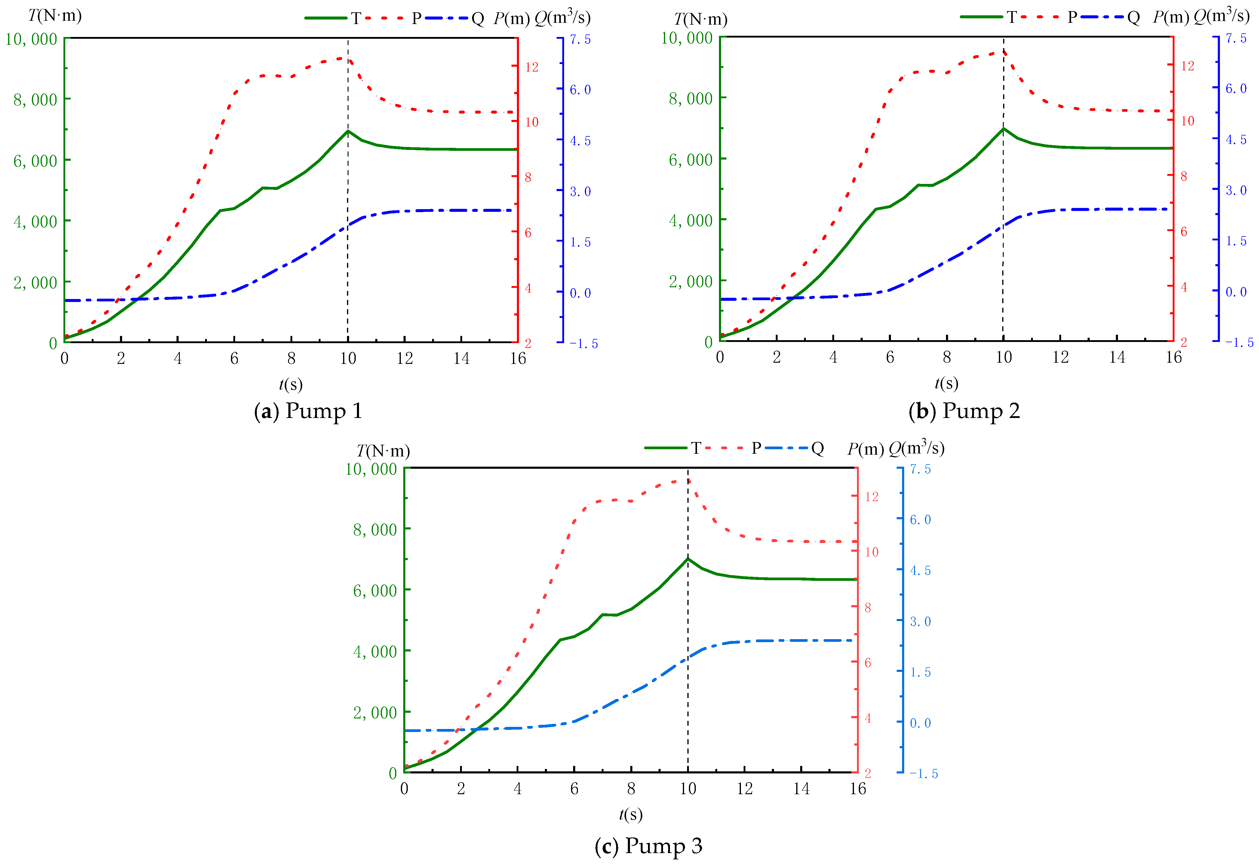
3.2.1. Simultaneous Pump Starting for Unit Set

When the valve is fully open, three operating units start linearly within 0–10 s simultaneously. The simulation results of pressure, flow rate, and torque variations with time for the three pumps are shown in Figure 7.

As shown in Figure 7, when three axial-flow pumps start simultaneously, the variation trends in torque, pressure, and flow rate in each pump during the startup process are essentially consistent. The head gradually increases before each pump reaches its rated speed, peaking at the moment of attaining rated speed with a maximum head of 12.59 m (23.43% above the rated head), while the torque also reaches its maximum value at this point. During simultaneous startup, reverse flow within the pumps progressively diminishes, being most severe during the initial startup phase with a maximum reverse flow of 0.26 m³/s (10.57% of the pump’s rated flow). These results demonstrate that the simultaneous startup of three pumps causes both pressure and reverse flow to exceed acceptable ranges. The pressure in particular surpasses the rated head by up to 23.43%, which explains why multi-pump simultaneous startup is generally avoided in practice. Such operation may induce excessive internal pressure, subjecting both pipelines and pumps to high-load impacts that could cause damage.

3.2.2. Unit Set Start-Up at 5 s Intervals Sequentially

When the valve is fully opened, the three operating units are linearly started at 5 s intervals, with the starting sequence as detailed in

Table 3. Pump valve starting modes.

Pump Valve Serial Number	Valve	Axial-Flow Pump
1	Fully open	Linear starting within 0–10 s
2		Linear starting within 5–15 s
3		Linear starting within 10–20 s

. Simulation calculations were performed, and the resulting pressure, flow rate, and torque variations of the three pumps over time are shown in Figure 8.

As can be seen from Figure 8, when the three units are started sequentially, the trends of head, flow rate, and torque of the three pumps are consistent. The maximum head occurs when the third pump reaches its rated speed, with an internal pump head of 11.36 m, exceeding the rated head by 11.41%. The first pump reaches its maximum head (11.10 m) upon attaining rated speed, after which it gradually decreases. A slight increase occurs at the 15 s mark when the second pump reaches its rated speed, followed by a second minor increase when the third pump reaches its rated speed, before stabilizing near the rated head. Similarly, the second pump exhibits a slight head increase when the third pump reaches rated speed, then decreases to near the rated head. The third pump only shows a peak head at the instant it reaches rated speed before gradually declining to near the rated head. The torque variation trend aligns with that of pressure. Similarly, the maximum reverse flow also occurs in the third pump. Severe reverse flow is observed during the initial pump start-up phase but diminishes as the pumps gradually stabilize. The maximum reverse flow reaches 0.34 m³/s, accounting for 13.87% of the pump’s rated flow. In summary, during the sequential start-up of the pumps at 5 s intervals, although the head decreases by 12.02% compared to simultaneous start-up, the maximum reverse flow increases by 3.30%.

3.2.3. Unit Set Start-Up at 15 s Intervals Sequentially

To further investigate the influence of sequential pump-start intervals on performance during parallel operation, the three units were started successively with the valve fully open. Pump 1 was initiated first, followed by Pump 2 after a 5 s delay upon completion of Pump 1’s start-up process, and so forth, resulting in a 15 s interval between each pump’s activation, as detailed in

Table 4. Pump valve starting modes.

Pump Valve Serial Number	Valve	Axial-Flow Pump
1	Fully open	Linear starting within 0–10 s
2		Linear starting within 15–25 s
3		Linear starting within 30–40 s

. This study examines the effects of start-up intervals on internal pump pressure, reverse flow, and internal flow field characteristics. The calculated variations in head, flow rate, and torque over time for each pump are presented in Figure 9.

As shown in Figure 9, when Pump 1 reaches its rated speed and stabilizes before starting Pump 2, its internal pressure and flow rate are still affected during the startup of other pumps. At the moments when Pump 2 and Pump 3 reach their rated speeds, Pump 1 experiences minor pressure fluctuations, while significant reverse flow persists—a phenomenon consistent with the 5 s interval startup scenario. Similarly, the maximum internal pressure (11.26 m) occurs during Pump 3’s startup, exceeding the rated head by 10.44%. This represents merely a 1% reduction compared to the 5 s interval scheme. The maximum reverse flow remains at 0.34 m³/s, showing no substantial improvement over the 5 s interval approach. These results demonstrate that extending the startup interval between pumps does not necessarily yield better performance.

3.2.4. Pump–Valve Coordination

When parallel-operating pump units adopt a “three-operating plus one-standby” configuration, initiating pump startup with the valve fully open may result in reverse flow reaching up to 13.87% of the pump’s rated flow capacity. Therefore, it is not advisable to fully open the valve prior to pump startup. Building upon previous research [23], this study proposes a 60% pre-opening valve design for parallel pump systems to investigate the effects of different valve opening strategies on internal pump pressure and flow characteristics. The specific valve opening schemes are detailed in

Table 5. Pump–valve starting modes.

Pump Valve Serial Number	Valve	Axial-Flow Pump
1	Initial opening degree: 0.6, fully opened from 0 to 10 s.	Linear starting within 0–10 s
2	Initial opening degree: 0.6, fully opened from 5 to 15 s.	Linear starting within 5–15 s
3	Initial opening degree: 0.6, fully opened from 10 to 20 s.	Linear starting within 10–20 s

and illustrated in Figure 10.

Numerical simulations were conducted for the aforementioned scheme, with the resulting variations in pressure, flow rate, and torque over time presented in Figure 10.

Figure 10 demonstrates that when implementing the valve opening strategy combining a 60% pre-opening with sequential pump startup (based on previous computational results), the three pumps exhibit nearly identical trends in head and torque variations over time. The maximum head (11.27 m) occurs when the third pump reaches rated speed, exceeding the rated head by 10.49%. For Pump 1, the peak head (11.03 m, 8.13% above rated) appears at its rated speed attainment, then gradually decreases until a minor increase to 10.83 m (6.16% above rated) occurs at 15 s when Pump 2 reaches rated speed. A second slight increase follows when Pump 3 attains rated speed, after which the head stabilizes near the rated value. Pump 2 shows similar behavior, with its head rising to 10.83 m during Pump 3’s speed synchronization before settling near the rated head. Pump 3’s head peaks only at its own rated speed attainment before gradually approaching the rated head. The torque variation closely follows the head fluctuation pattern. The maximum reverse flow (0.15 m³/s, 6.04% of rated flow) occurs during Pump 3’s initial startup phase, representing a 7.83% reduction compared to the non-pre-opened valve scenario, demonstrating significant improvement.

To further investigate the internal flow characteristics during the pump startup process, a comparative analysis was conducted on the flow patterns at the radial coefficient r = 0.5 of the impeller for three scenarios: (1) the instant of each pump’s startup, and (2) stable operation after all three pumps were fully started. The schematic diagram of the impeller cross-section at radial coefficient r = 0.5 is shown in Figure 11, while the corresponding internal flow patterns are presented in Figure 12.

Figure 12a–c illustrates the internal flow characteristics at the impeller’s radial coefficient r = 0.5 for Pump 1 under four operational conditions: (1) at the instant of reaching rated speed during startup (10 s), (2) when Pumps 2 and 3 attain rated speed during their startups (15 s and 20 s, respectively), and (3) during stable operation after all three pumps are fully started (25 s), with consideration of valve effects. The results demonstrate that when Pump 2 is started 5 s after Pump 1’s initiation, Pump 1’s internal flow characteristics during subsequent pump startups remain consistent with those observed during its own startup. The pressure distribution shows relative uniformity, with localized high-pressure zones appearing near the discharge side of the blade’s back surface at the instant of rated speed attainment. During the rated speed attainment of Pumps 2 and 3, Pump 1’s flow field experiences disturbances, manifesting as small high-pressure zones on the blade’s back surface and localized high turbulent kinetic energy regions near the trailing edge. These flow instabilities diminish after Pumps 2 and 3 complete their startups. The maximum flow velocity (normalized value: 0.9823) and turbulent kinetic energy (0.9022 m²/s²) occur during Pump 1’s startup phase, representing reductions of 3.69% and 10.27%, respectively, compared to the non-pre-opened valve scenario. The peak pressure also decreases by 2.65%, collectively demonstrating enhanced flow stability within the pump.

Figure 12d–f show the internal flow characteristics at the radial coefficient r = 0.5 of the impeller blades for Pump 2 at the moment when it reaches the rated speed (15 s), Pump 3 at the moment when it reaches the rated speed (20 s), and when all three pumps are started and operating stably (25 s). It can be seen from the figure that the internal flow condition of Pump 2 when Pump 3 starts and reaches the rated speed is consistent with that when it starts and reaches the rated speed. Compared with stable operation, the internal pressure gradient is larger. At the moment when Pump 2 starts and reaches the rated speed, there is a high-pressure area on the back of the impeller blades, and the non-dimensional pressure extreme value reaches 1.6798. At this time, the pressure difference of the impeller is large, and the stress on the blades is large. Compared with the internal flow condition of Pump 2 during stable operation, the internal flow state of the impeller is worse. There is a small area of high turbulent kinetic energy at the tail of the impeller blades, and slight flow separation occurs. At the moment when Pump 3 starts and reaches the rated speed at 20 s, a small high-speed area appears in Pump 2, and the maximum non-dimensional flow velocity is 0.9622. As Pump 3 completes the start-up, the internal flow condition of the pump returns to stability. Compared with the pump starting mode without pre-opening the valve, when the valve is pre-opened to 60% open, the pressure fluctuation in the pump is less, the high-pressure area and high-speed area are also less. The maximum pressure decreases by 3.70%, the flow velocity decreases by 1.26%, and the overall situation is improved.

Figure 12g–i illustrate the internal flow characteristics at the radial coefficient r = 0.5 of the impeller blades for Pump 3 at the moment when it reaches the rated speed (20 s) and when all three pumps are started and operating stably (25 s). As shown in the figure, compared with stable operation, the internal pressure gradient of Pump 3 is larger when it starts and reaches the rated speed. The high-pressure area is concentrated at the outlet end of the impeller on the back of the blades. At this time, the internal flow of the impeller is relatively unstable, and the internal flow state of the impeller is worse than that during stable operation. There is a small area of high turbulent kinetic energy at the tail end of the impeller blades, where slight flow separation occurs. Combined with

Table 6. Extreme values of non-dimensional pressure, non-dimensional velocity, non-dimensional turbulent kinetic energy at impeller radial coefficient r = 0.5 during start-up and stable operation of each pump.

Parameter	Pump	Start-Up of Pump 1 (10 s)	Start-Up of Pump 2 (25 s)	Start-Up of Pump 3 (40 s)	Stable Operation (45 s)
Pressure	Pump 1	1.7728	1.7152	1.7736	1.7741
	Pump 2	-	1.6798	1.6939	1.7501
	Pump 3	-	-	1.7249	1.6906
Velocity	Pump 1	0.9823	0.9460	0.9574	0.9540
	Pump 2	-	0.9718	0.9622	0.9158
	Pump 3	-	-	0.9867	0.9096
Turbulent Kinetic Energy	Pump 1	0.9022	0.9070	0.9103	0.9619
	Pump 2	-	1.0240	0.9207	1.0931
	Pump 3	-	-	1.0786	0.9422

, it can be seen that the maximum non-dimensional pressure of Pump 3 reaches 1.7249. At the moment when Pump 3 reaches the rated speed, the maximum pressure in the pump is also higher than that when all three pumps are stably operating. The maximum flow velocity in the impeller reaches 27.123 m/s, but as Pump 3 completes the start-up, the internal flow condition of the pump returns to stability. Compared with the pump-starting mode without pre-opening the valve, when the valve is pre-opened to 60% open, the pressure fluctuation in the pump is less, the high-pressure area and high-speed area are also less, and the internal flow condition of the pump is more stable.

To further analyze the variation in pressure pulsation characteristics in the internal flow field of the axial-flow pump during the coordinated start-up of the unit and valve, the internal flow characteristics at the impeller r = 0.5 are selected for pressure pulsation acquisition at the moment when the pump starts and reaches the rated speed, the moment when other pumps reach the rated speed, and during stable operation. The rotational speed of the axial-flow pump at rated speed is 750 rpm. The pressure distribution characteristics at every 2° during the impeller rotation are collected with a sampling time step of 0.000444 s. The analysis samples are the pressure data after the pump rotates steadily for 4 cycles. To monitor the pressure pulsation in the pump, monitoring points P1–P3, P4–P6, P5–P9, P10–P12, P13–P15, and P16–P18 are radially arranged on the sections of the impeller inlet, impeller mid-span, impeller outlet, guide vane inlet, guide vane mid-span, and guide vane outlet of the axial-flow pump, respectively. The distribution of monitoring points is shown in Figure 13.

$$C_p={\displaystyle \frac{P-\overline{P}}{0.5\rho u_2^2}}$$

(11)

$$u_2={\displaystyle \frac{n\pi D_2}{60}}$$

(12)

Figure 14a–d shows the pressure pulsation variations at the impeller internal detection points of Pump 1 at the moment when it reaches the rated speed (10 s), when Pumps 2 and 3 reach the rated speed (15 s and 20 s), and during stable operation (25 s).

Table 7. Statistical table of pressure pulsation characteristics at different monitoring points in impeller of Pump 1.

	Monitoring Point	Dominant Frequency	Amplitude	Secondary Frequency	Amplitude
10 s	P4	12.5	0.0058	25.0	0.0016
	P5	12.5	0.0058	25.0	0.0015
	P6	12.5	0.0058	25.0	0.0016
15 s	P4	12.5	0.0028	25.0	0.0021
	P5	12.5	0.0027	25.0	0.0020
	P6	12.5	0.0032	25.0	0.0022
20 s	P4	12.5	0.0028	25.0	0.0021
	P5	12.5	0.0027	25.0	0.0020
	P6	12.5	0.0032	25.0	0.0022
25 s	P4	12.5	0.0010	25.0	0.0004
	P5	12.5	0.0010	25.0	0.0004
	P6	12.5	0.0011	25.0	0.0005

presents the statistical data of pressure pulsation at different monitoring points in the impeller of Pump 1. Combining Figure 14a–d and Table 7, it can be seen that the dominant frequency of pressure pulsation at each point is the rotation frequency, and the secondary frequency is twice the rotation frequency, indicating that the pressure fluctuations in the system are mainly caused by impeller rotation. The amplitude at the monitoring points during stable operation of the pump is the smallest, only 0.001. At the moment when Pump 1 reaches the rated speed at 10 s, the amplitude of pressure pulsation in the pump is greater than that during stable operation, but only exceeds it by about 0.0048. At the moment of pump start-up, the amplitudes of pressure pulsation at each point are basically equal, indicating that the pressure fluctuations are relatively uniform on this plane. Combining with the pressure nephogram and velocity nephogram, it can be seen that there is a small high-pressure area at the outlet end of the impeller on the back of the blades at this time. At the moments when Pumps 2 and 3 start and reach the rated speed at 15 s and 20 s, the amplitudes in the pump are also slightly larger than the pressure amplitudes during stable operation of the pump, only exceeding by 0.002, which corresponds to the pressure field, velocity field, and turbulent kinetic energy nephograms in the pump. At this time, the pressure distribution in the pump is relatively uniform. After all parallel units are started up at 25 s, the amplitude in the pump stabilizes at about 0.001. Combining with the nephograms, it can be seen that the pressure and velocity distributions in the pump are uniform at this time, and the small high-turbulent kinetic energy area at the tail end of the impeller blades also disappears, so the internal flow condition of the pump is more stable.

Figure 14e–g show the pressure pulsation variations at the impeller internal detection points of Pump 2 at the moment when it reaches the rated speed (15 s), when Pump 3 reaches the rated speed (20 s), and during stable operation (25 s).

Table 8. Statistical table of pressure pulsation characteristics at different monitoring points in impeller of Pump 2.

	Monitoring Point	Dominant Frequency	Amplitude	Secondary Frequency	Amplitude
15 s	P4	12.5	0.0018	25.0	0.0007
	P5	12.5	0.0012	25.0	0.0008
	P6	25.0	0.0011	12.5	0.0008
20 s	P4	12.5	0.0043	25.0	0.0022
	P5	12.5	0.0041	25.0	0.0021
	P6	12.5	0.0045	25.0	0.0023
25 s	P4	12.5	0.0010	25.0	0.0004
	P5	12.5	0.0010	25.0	0.0004
	P6	12.5	0.0011	25.0	0.0005

presents the statistical data of pressure pulsation at different monitoring points in the impeller of Pump 2. Combining Figure 14e–g and Table 8, it can be seen that the dominant frequency of pressure pulsation at each point is the rotation frequency, except that P6 at 20 s is the 2× frequency, and the secondary frequency is the 2× rotation frequency, except that P6 at 20 s is the rotation frequency, indicating that the pressure fluctuations in the system are mainly caused by impeller rotation. The amplitude at the monitoring points during stable operation of the pump is the smallest, only 0.001, the same as that of Pump 1. At the moment when Pump 2 reaches the rated speed at 15 s, the amplitude of pressure pulsation in the pump is greater than that during stable operation, but only exceeds it by about 0.0008. At the moment of pump start-up, the amplitudes of pressure pulsation at each point are basically equal, indicating that the pressure fluctuations are relatively uniform on this plane. Combined with the pressure nephogram and velocity nephogram, it can be seen that there is a small high-pressure area at the outlet end of the impeller on the back of the blades at this time. At the moment when Pump 3 starts and reaches the rated speed at 20 s, the amplitude in the pump is also slightly larger than the pressure amplitude during stable operation of the pump, only exceeding it by 0.003, which corresponds to the pressure field, velocity field, and turbulent kinetic energy nephograms in the pump. At this time, the pressure distribution in the pump is relatively uniform. After all parallel units are started up at 25 s, the amplitude in the pump stabilizes at about 0.001. Combining with the nephograms, it can be seen that the pressure and velocity distributions in the pump are uniform at this time, and the small high-turbulent kinetic energy area at the tail end of the impeller blades also disappears, so the internal flow condition of the pump is more stable.

Figure 14h–i show the pressure pulsation variations at the impeller internal detection points of Pump 3 at the moment when it reaches the rated speed (20 s) and during stable operation (25 s).

Table 9. Statistical table of pressure pulsation characteristics at different monitoring points in impeller of Pump 3.

	Monitoring Point	Dominant Frequency	Amplitude	Secondary Frequency	Amplitude
20 s	P4	25.0	0.0030	12.5	0.0020
	P5	25.0	0.0026	12.5	0.0022
	P6	12.5	0.0026	25.0	0.0021
25 s	P4	12.5	0.0010	25.0	0.0004
	P5	12.5	0.0010	25.0	0.0004
	P6	12.5	0.0012	25.0	0.0005

presents the statistical data of pressure pulsation at different monitoring points in the impeller of Pump 2. Combining Figure 14h–i and Table 9, it can be seen that the dominant frequency of pressure pulsation at each point is the rotation frequency, except that P4 and P5 at 20 s are the 2× frequency, and the secondary frequency is the 2× rotation frequency, except that P4 and P5 at 20 s are the rotation frequency, indicating that the pressure fluctuations in the system are mainly caused by impeller rotation. The amplitude at the monitoring points during stable operation of the pump is the smallest, only 0.001, the same as that of Pumps 1 and 2. At the moment when Pump 3 reaches the rated speed at 20 s, the amplitude of pressure pulsation in the pump is greater than that during stable operation, but only exceeds it by about 0.001. At the moment of pump start-up, the amplitudes of pressure pulsation at each point are basically equal, indicating that the pressure fluctuations are relatively uniform on this plane. Combining with the pressure nephogram and velocity nephogram, it can be seen that there is a small high-pressure area at the outlet end of the impeller on the back of the blades at this time. After all parallel units are started up at 25 s, the amplitude in the pump stabilizes at about 0.001. Combining with the nephograms, it can be seen that the pressure and velocity distributions in the pump are uniform at this time, and the small high-turbulent kinetic energy area at the tail end of the impeller blades also disappears, so the internal flow condition of the pump is more stable.

When the parallel operation unit is started in conjunction with the valve and each pump is started sequentially at an interval of 5 s with the connected valve opening pre-opened to 60%, the pressure in the pump exceeds 10.49% of the rated head of the pump, which is 0.92% lower than the scheme of starting at the same time without matching the valve. The maximum backflow reaches 6.04% of the rated flow of the pump, which is 7.83% lower than the scheme of starting the pump at the same time without matching the valve. Studies have shown that the influence of the pre-opening degree of the valve on the internal and external characteristics of the pump still exists when the pumps are in parallel operation. When the valve is pre-opened to 60% during the parallel operation of each pump, the backflow in the pump is significantly improved. Comprehensive analysis of internal flow characteristics such as pressure, velocity, and turbulent kinetic energy shows that the high-pressure area on the back of the blade is significantly improved; the backflow phenomenon no longer occurs at the outlet end of the impeller at the tail of the blade, and the high turbulent kinetic energy area is significantly reduced. Combined with the pressure pulsation, it is found that the pressure distribution in the pump is relatively uniform and the flow in the pump is more stable. Therefore, when starting the pump in parallel operation of the unit, it is also recommended to pre-open the valve behind the pump to 60% open before starting the pumps one by one. Under the same conditions, the interval time for starting the pumps one by one is not as long as possible, and the starting time can be shortened as much as possible without affecting the pressure in the pump.

4. Conclusions

This paper adopts a 1D–3D coupling method to investigate the effects of pump start-up on internal pressure, flow rate, etc., of four axial-flow pumps in parallel operation under the condition of “three units in operation and one unit on standby”. The start-up scenarios include four cases: simultaneous start-up of three operating pumps, start-up with 5 s intervals, start-up with 15 s intervals, and start-up with 5 s intervals in conjunction with valve coordination. By observing the internal pressure field, velocity field, and turbulent kinetic energy nephograms of the pumps, monitoring the pressure pulsation in the impellers, and combining with 1D simulation, the following conclusions are drawn:

(1) When the parallel operation units are started simultaneously, large pressure and backflow occur in the pumps. The maximum pressure exceeds 23.43% of the rated head of the pump, and the maximum backflow reaches 10.57% of the rated flow of the pump. Both the internal pressure and backflow of the pump exceed the reasonable range. Therefore, the method of starting multiple units simultaneously is usually not adopted in practical applications, as it is prone to cause excessive pressure in the pump, resulting in high-load impact on the pipeline and pump, and causing damage.

(2) When the parallel operation units are started simultaneously, large pressure and backflow occur in the pumps. The maximum pressure exceeds 23.43% of the rated head of the pump, and the maximum backflow reaches 10.57% of the rated flow of the pump. Both the internal pressure and backflow of the pump exceed the reasonable range. Therefore, the method of starting multiple units simultaneously is usually not adopted in practical applications, as it is prone to cause excessive pressure in the pump, resulting in high-load impact on the pipeline and pump causing damage.

(3) When the parallel operation units are started in conjunction with the valve pre-opened to 60%, the internal pressure of the pump exceeds 10.49% of the rated head, which is 0.92% lower than the scheme without valve coordination, and the maximum backflow decreases by 7.83%. Studies show that the backflow in the pump is significantly improved. According to the internal flow characteristics, the high-pressure area on the back of the blade is obviously alleviated, and the high turbulent kinetic energy region is significantly reduced. Combined with the pressure pulsation, it is found that the internal pressure distribution of the pump is relatively uniform and the flow condition is more stable. Therefore, when starting up parallel operation units, it is recommended to pre-open the valve behind the pump to 60% open before starting the pumps one by one. Under the same conditions, the interval time for sequential start-up should not be too long, and the start-up time can be shortened as much as possible without affecting the internal pressure of the pump.

References

1. Meng, F.; Qin, Z.J.; Li, Y.J.; Chen, J. Investigation of Transient Characteristics of a Vertical Axial-Flow Pump with Non-Uniform Suction Flow. Machines 2022, 10, 855. [Google Scholar] [CrossRef]
2. Jing, R.; He, X.J. Overview of Axial Flow Pumps and Their Applications. Gen. Mach. 2014, 4, 86–89. [Google Scholar]
3. Fu, S.; Zheng, Y.; Kan, K.; Chen, H.; Han, X.; Liang, X.; Liu, H.; Tian, X. Numerical simulation and experimental study of transient characteristics in an axial flow pump during start-up. Renew. Energy 2020, 146, 1879–1887. [Google Scholar] [CrossRef]
4. Meng, S.; Sun, C.; Li, Y.; Zhang, Y.; Pang, X. Research on the Evaluation Method for Pumping Performance of Large-Scale Parallel Vacuum Systems. Vacuum 2025, 3, 1–7. [Google Scholar]
5. Cui, Y.; Wang, Z. Engineering Practice for Achieving High-Efficiency Operation of Multi-Pump Parallel Systems. Gas Heat 2024, 44, 14–23. [Google Scholar]
6. Gan, X.; Gong, X.; Pei, J.; Pavesi, G.; Yuan, S. Machine Learning Approaches for Enhancing Energy Efficiency and Stability in Parallel Pumping Systems. Water Resour. Manag. 2024, 39, 1719–1746. [Google Scholar] [CrossRef]
7. Zhao, K.; Wang, T.; Shang, Y.; Song, J.; Chen, J.; Liu, L. Reliability-Based Optimization Study on Pump Addition/Cutback in Parallel Pump Systems. Water Resour. Power 2024, 42, 149–153. [Google Scholar]
8. Cong, W.; Ge, H.; Cheng, J.; Zhang, S. Optimal allocation model and method for parallel ‘reservoir and pumping station’ irrigation system under insufficient irrigation conditions. Appl. Water Sci. 2023, 13, 199. [Google Scholar] [CrossRef]
9. Hou, S.; Yu, J.; Su, Y.; Liu, Z.; Dai, J. Flow distribution optimization of parallel pumps based on improved mayfly algorithm. J. Intell. Fuzzy Syst. 2023, 44, 2065–2083. [Google Scholar] [CrossRef]
10. Wang, G.; Ghoddousi, S.; Wang, Z.; Song, L. Development, validation and application of an energy model for energy efficient operation of parallel pump systems. J. Build. Eng. 2022, 59, 105098. [Google Scholar] [CrossRef]
11. Guo, T.; Xiao, W.; Liu, J.; Fu, Y. Research on Oil Return Interference in the Casing of Multi-Pump Parallel Hydraulic Systems for Large Aircraft. Adv. Aeronaut. Sci. Eng. 2025, 1–13. [Google Scholar]
12. Behroozi, M.A.; Vaghefi, M. Numerical Investigation of Water Hammer due to Transient in Parallel Pumps. Int. J. Civ. Eng. 2021, 19, 1415–1425. [Google Scholar] [CrossRef]
13. Yang, Z.; Zhou, L.; Dou, H.; Lu, C.; Luan, X. Water hammer analysis when switching of parallel pumps based on contra-motion check valve. Ann. Nucl. Energy 2020, 139, 107275. [Google Scholar] [CrossRef]
14. Özkayar, G.; Wang, Z.; Lötters, J.; Tichem, M.; Ghatkesar, M.K. Flow Ripple Reduction in Reciprocating Pumps by Multi-Phase Rectification. Sensors 2023, 23, 6967. [Google Scholar] [CrossRef]
15. Tian, D.; Si, Q.; Liang, K.; Zhang, Y.; Ju, Y.; Yuan, J. Study on the Internal Flow Characteristics of High Flowrate Emergency Drainage Series-parallel Pump. J. Phys. Conf. Ser. 2024, 2854, 12062. [Google Scholar] [CrossRef]
16. Carricondo-Antón, J.M.; Jiménez-Bello, M.A.; Juárez, J.M.; Tomas, A.R.; González-Altozano, P. Optimization of an isolated photovoltaic water pumping system with technical–economic criteria in a water users association. Irrig. Sci. 2023, 41, 817–834. [Google Scholar] [CrossRef]
17. Gasque, M.; González-Altozano, P.; Gutiérrez-Colomer, R.P.; García-Marí, E. Comparative evaluation of two photovoltaic multi-pump parallel system configurations for optimal distribution of the generated power. Sustain. Energy Technol. Assess. 2021, 48, 101634. [Google Scholar] [CrossRef]
18. Oh, H.; Guk, I.; Chung, S.; Lee, Y. Energy saving through modifications of the parallel pump schedule at a pumping station: A case study. J. Water Process Eng. 2023, 54, 104035. [Google Scholar] [CrossRef]
19. Manickavel, B.; Raja, R.S. AI Energy Optimal Strategy on Variable Speed Drives for Multi-Parallel Aqua Pumping System. Energies 2022, 15, 4343. [Google Scholar] [CrossRef]
20. Wang, Y.; Li, S. Analysis of Parallel Operation of Axial Flow Pumps. Pump Technol. 2022, 4, 5–8. [Google Scholar]
21. Zhou, L. Operation Optimization of Pumping Stations with Multiple Parallel Pumps. J. Irrig. Drain. 2014, 33, 96–99. [Google Scholar]
22. Song, Y. Investigation on Transient Flow Mechanism in Pump-Turbine Units Based on 1D-3D Coupling Method. Harbin Inst. Technol. 2022. [Google Scholar]
23. Fu, Y.; Deng, L. The Influence of Pre-Lift Gate Opening on the Internal and External Flow Characteristics During the Startup Process of an Axial Flow Pump. Processes 2024, 12, 1984. [Google Scholar] [CrossRef]
Figure 1. Schematic diagram of the axial-flow pump water model.
Water 17 02285 g001
Figure 2. Schematic diagram of pump units in parallel operation.
Water 17 02285 g002
Figure 3. The mesh for main components.
Water 17 02285 g003
Figure 4. Mesh independence verification.
Water 17 02285 g004
Figure 5. Schematic diagram of mesh independence verification.
Water 17 02285 g005
Figure 6. Experimental validation of the model pump. (a) Schematic diagram of axial-flow pump experiment setup. (b) Comparison of calculated and experimental values.
Water 17 02285 g006
Figure 7. Time–variation graphs of pressure, flow rate and torque.
Water 17 02285 g007
Figure 8. Time–variation graphs of pressure, flow rate and torque.
Water 17 02285 g008
Figure 9. Time–variation graphs of pressure, flow rate and torque.
Water 17 02285 g009
Figure 10. Time–variation graphs of pressure, flow rate and torque.
Water 17 02285 g010
Figure 11. At the radial coefficient r = 0.5 of the impeller.
Water 17 02285 g011
Figure 12. Internal flow characteristics at impeller r = 0.5 of Pump 1, Pump 2, Pump3.
Water 17 02285 g012
Figure 13. Distribution of monitoring points.
Water 17 02285 g013
Figure 14. Frequency domain diagrams of pressure pulsation in impeller of Pump 1, Pump 2, Pump 3.
Water 17 02285 g014aWater 17 02285 g014b