Article

Laboratory Assessment for Determining Microplastics in Freshwater Systems—Characterization and Identification along the Somesul Mic River

by
Stefania Gheorghe
1,*,†,
Catalina Stoica
1,†,
Anca Maria Harabagiu
1,
Dorian-Gabriel Neidoni
2,
Emanuel Daniel Mighiu
1,
Costel Bumbac
1,
Ioana Alexandra Ionescu
1,
Aida Pantazi
3,
Laura-Bianca Enache
3 and
Marius Enachescu
3
1
Control Pollution Department, National Research and Development Institute for Industrial Ecology—ECOIND 57-73 Drumul Podu Dambovitei, Sector 6, 060652 Bucharest, Romania
2
National Research and Development Institute for Industrial Ecology—ECOIND, Bujorilor Street, 115, Timis District, 300431 Timisoasa, Romania
3
Center for Surface Science and Nanotechnology, National University of Science and Technology Polytechnic Bucharest, 313 Splaiul Independentei, AN031, District 6, 060042 Bucharest, Romania
*
Author to whom correspondence should be addressed.
These authors contributed equally to this work.
Water 2024, 16(2), 233; https://doi.org/10.3390/w16020233
Submission received: 29 November 2023 / Revised: 19 December 2023 / Accepted: 26 December 2023 / Published: 9 January 2024
(This article belongs to the Section Water Quality and Contamination)

Abstract

:
Microplastics (MPs) pollution has become a persisting problem over the last decades and is a critical issue for environmental protection and human health. In this context, scientific data able to reveal MPs presence and improve the characterization and identification of this pollution via different systems are valuable. The aim of this paper is to assess available techniques for determining MPs in real freshwater samples and subsequently to highlight the occurrence and type of MPs in the study case area (Somesul Mic River). The MPs sampling was performed from fresh water and sediment using planktonic nets and sieves with different mesh sizes (from 20 to 500 µm). Using both classical microscopic techniques as well as scanning electron microscopy (SEM), large (1–5 mm) and small (1 µm to 1 mm) MPs were observed in the shape of fibers, fragments, foam, foils and spheres in various colors (red, green, blue, purple, pink, white, black, transparent, and opaque). Raman and FT-IR spectroscopic methods were used for MPs identification. The presence of polyethylene (PE), polypropylene (PP), and polystyrene (PS) was registered for all sampling points. The MPs laboratory investigations have raised some issues regarding the identification of MPs particles smaller than 500 µm, these being characterized especially under microscope. Some small MPs particles were identified using micro-Raman spectroscopy that highlighted the same type of polymers. No differences were registered between the sampling points due to the widespread presence of MPs. The sediment samples presented a greater abundance as compared to the water samples. Overall, it is necessary to continue the optimization of MPs separation protocol and identification according to the complexity of samples, mainly due to the limitation and lack of spectral databases.

1. Introduction

Plastic pollution is considered one of the main problems of our century as it is a worldwide concern [1,2]. According to ISO/DIS 24187:2021(E), plastics represent a material that contains, as an essential ingredient, a high polymer and which, at some stage in its processing into finished products, can be shaped by flow [3]. Due to the large utility of plastics and poor waste management, they can lead to the contamination of most environmental systems [4,5,6,7]. Aquatic systems are the most affected ones. Research media and global organizations have raised alarm signals concerning the accumulation of plastics in the oceans, seas, and freshwater systems. The results of plastic degradation in the environment or in wastewater treatment systems are classified in terms of the longest distance of the particle: macroplastics (above 5 cm), small macroplastics (5 mm to 5 cm), large microplastics (1 mm to 5 mm), microplastics (1 µm to 1 mm), and nanoplastics (less than 1 µm) [3]. They represent any solid plastic insoluble in water and are found in various shapes. The principal sources of MPs are: the breakdown of plastic products such as packaging materials, the microspheres in personal care products (detergents, exfoliants, toothpaste, sunscreens, etc.), fibers from synthetic textiles, tire wear microparticles, city dust (resulted from plastic litter fragmentation), electrical and electronics materials, building and construction sector debris, and agriculture processes. Other sources are the municipal/industrial sewage sectors because even wastewater treatment plants (WWTP) are not designed to properly retain microplastics [8,9].
The occurences of plastic pollution tend to escalate, and even if plastic use was stopped immediately, the pollution would continue to persist due to the very low capacity of environmental factors and microbiomes to biodegrade these polymers (for example, polyethylene needs between <400 and >800 years to degrade [10]). The problem has become even more critical with the increase of plastics use due to our urge to cope with the protection requirements imposed by the COVID-19 pandemic (gloves, gowns, masks, glasses, etc.). The International Solid Waste Association estimated 250–300% more consumption of single-use plastic materials during the pandemic, and the World Health Organization (WHO) estimated a consumption of 89 million medical masks per month [11]. It was estimated that the global annual leakage of macroplastics will increase from 19.4 mt in 2019 to 38.4 mt in 2060, while the leakage of microplastics will double, to reach 5.8 mt in 2060 [12]. In Europe, the production of plastics has reached almost 58 million tons [13].
Pollution with plastic/microplastic materials has often been reported in rivers worldwide (Rhine, Danube, Elbe, the Yellow River, the Amazon, etc.) [14,15,16,17,18] as well as other freshwater systems that are used as drinking water sources [19,20,21]. The abundance of MPs in freshwater systems has been reported to vary, depending on sample sources, from 10−3 to 103 particles/L [22] or to over 104 particles per liter, with a particle size distribution of 95% in the size range of 6.5 and 100 µm [23] to absolute concentrations of 0.008 mg/L to 0.039 mg/L [24]. The abundance of MPs in sediments has been reported to be less than 87 particles kg−1 in the Danube River: Iron Gate, from 87 to 165 particles kg−1 in the Danube Delta, and 630 particles kg−1 in the marine sediment of the Black Sea [25,26]. Some prospective studies showed that, in certain conditions of low-flow and sandy sediment, MPs build up in concentrations of 3.6 to 10.7 particle/L in water and 360 to 1320 items/Kg in sediment; higher concentrations have been registered in the samples collected from sites neighboring densely populated areas or extensive agricultural planting areas [27].
According to the PlaticsEurope statistics (2022), in 2021, polypropylene (PP) and polyethylene (PE) were the most-demanded polymer types. Approximately 19.3% was PP, more than 20% was PE (low- and high-density), 5.3% was PS (polystyrene), and 6.3% was PET (polyethylene terephthalate). These plastics were predominantly used in diverse activities, especially in packaging and construction activities. However, only 10% of these plastics were recycled, and only 1.5% bio-based plastics were produced [28].
Most studies have reported the occurrence of common synthetic polymers such as PE and PS, among others, in surface waters [16,29,30,31]. The composition of microplastic pollution can vary in terms of polymer types, colors, and additives used in plastics, and, of course, depends on the sources and local factors. For example, in urban areas, microplastics from personal care products and synthetic textiles may be more prevalent, while in coastal regions, microplastics from degraded fishing nets and maritime debris can be significant contributors [32,33]. For almost 10 years, even in apparently non-polluted areas far from the civilization, scientific reports have revealed the occurrence of PP, PE, and PS as the most prevalent MPs in the surface water or sediment [34,35].
In the Danube River, the most important river in Romania, PP and PE have been reported as the main MP pollutants, probably due to their various applications, especially in the packaging industry [26].
Recent studies focusing on the assessment of MPs effects and impact on living organisms, including humans, showed that the main hazards with microplastics for the environment, especially in aquatic ecosystems, are as follows: physical effects, bioaccumulation, desorption and toxicity of pollutants, leaching and toxicity of additives and monomers, and transport of invasive species [21]. Moreover, if we consider the absorption potential of the MPs surface area, the concern regarding potential environmental and health impacts increases as the MPs would become carriers of other, potentially more harmful pollutants. A series of polluting chemical compounds such as metals, pesticides, or pharmaceutical substances can be absorbed on their surfaces, thus increasing their toxic effects [13].
Some statistical studies have reported the presence of MPs in different food sources like meat, seafood, bottled and tap drinking water, beverages, sugar, salt, honey, and milk [8,21,36].
The small size and diversity of MPs’ physical and chemical properties raise problems regarding their characterization and detection in environmental samples and biota. Currently, the recommended techniques for the morphological characterization of MPs are visual analysis, classical microscopic investigation (especially for large particles 1–5 mm), and SEM-scanning electron microscopy analysis (applied for small particles <1 mm). For the MPs identification spectroscopy investigations can be applied even for ≤1 mm particle size. According to the literature, these MPs detection methods have advantages and limitations, and some are time- and cost-consuming. There is a lack of harmonized procedures from sampling and sample preparation to detection analyses. Other inconveniences include human error and lack of expertise. Micro-Raman or FT-IR spectroscopy, although expensive, are automated systems that are recognized as being more reliable and precise and could contribute to reducing both analysis time and human error [37,38,39]. Also, the literature report other suitable techniques for characterizing the presence of microplastic in freshwater ecosystems such as biomonitoring studies using DNA metabarcoding [40], the employment of single-molecule techniques [41], and computer simulation approaches [42]. However, these techniques also include inconveniences, such as the limitation of biomarker availability, the complexity of calibration steps prior to data acquisition, and the need for large datasets linked to computational cost resources.
The aim of the present study is to assess available techniques for MPs detection and to reveal the presence and type of MPs in the freshwater systems of Romania (study case Somesul Mic River, section Floresti-Cluj-Napoca).

2. Material and Methods

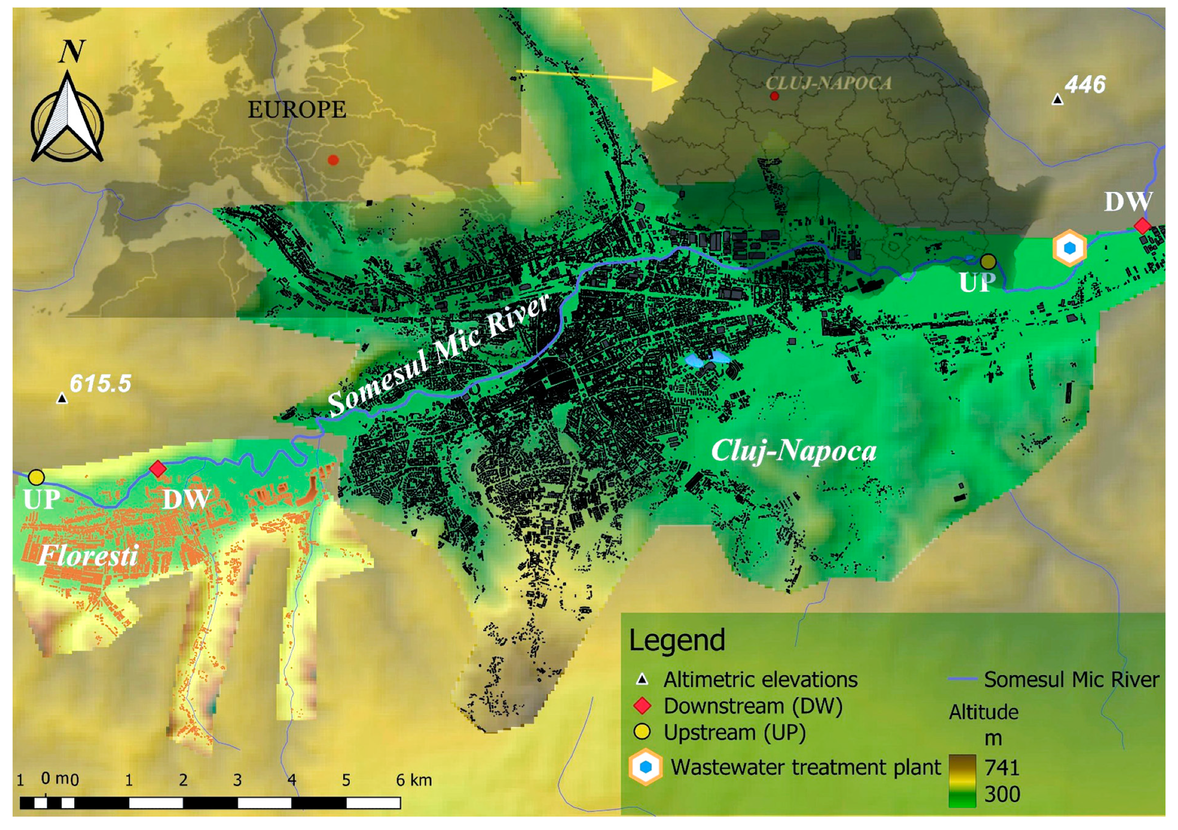
2.1. Experimental Design

To highlight MPs contamination in freshwater, a sampling campaign was initiated in the Northwest area of Romania in September 2022 for 1 day. The Somesul Mic River runs through the city of Cluj-Napoca and its outskirts, including the town of Floresti. Four sampling points were selected along the river: upstream (UP) and downstream (DW) of Floresti (sampling point codes: UP Floresti and DW Floresti), and upstream and downstream of the Cluj-Napoca Wastewater Treatment Plant (sampling point codes: UP Cluj-Napoca WWTP and DW Cluj-Napoca WWTP) (Figure 1).
The Somesul Mic River has an average flow rate of 21.2 m2/s, passes through densely populated areas, and flows into the Mures River, which is an important cross-border water body with a route to Hungary that discharges into the Tisa River. The investigated area represents an urban environment with industrial, zoological, technical, and tourist activities. The city of Cluj-Napoca (46°46′0″ N 23°35′0″ E) covers an area of 179.5 km2 and has a population of 324,576 inhabitants, while the metropolitan area includes 410,766 inhabitants. Cluj-Napoca was chosen as the study area based on both its ranking in terms of quality of life (Cluj-Napoca ranked 43rd out of 91 European cities studied at the beginning of 2021) and the dynamics of the city’s economy as compared to the national level. Floresti (46°44′52″ N 23°29′27″ E) covers an area of 61 km2, with a population of approximately 50,000 inhabitants, a population that is growing due to expansion as it is a suburb of Cluj-Napoca that is experiencing ongoing real estate development. Potential sources of plastic pollution in these areas include construction sites, household waste, and economic activities, as well as improperly stored household waste and the Cluj-Napoca wastewater treatment plant (https://ro.wikipedia.org, accessed on 10 March 2023).
The sampling sites were chosen along the river’s flow direction, as this is geomorphologically favorable for sediment deposition. Additionally, the sampling point selections were based on inspections of the left bank of the river (depending on the area accessibility) and possible sources of contamination with plastic materials. Visual inspections of the riverbanks revealed the presence of plastic waste in the selected areas, which was mostly of household or construction origin (Figure S2).

2.2. Sampling Technique

The EPA Microplastics Sampling Protocol [39], the Rocha International Sampling Guide [43], and other review studies on the sampling, pretreatment, and analysis of MPs [6,44,45] were consulted for the organization of the sampling campaign. The sampling protocol was also adapted based on the requirements of ISO/DIS 24187:2022 [7].
For each sampling site, three different sample units of surface water and sediment were collected.
The surface water samples were collected directly from the river and concentrated by filtration using two methods: (1) by passing approximately 100 L of water using a 10 L bucket through plankton nets with mesh sizes of 20 and 200 µm, respectively, (Pokorny Site, Nitex, Czech Republic) and then individually collecting the samples in 100 mL glass vials; and (2) by placing the nets against the direction of river flow for 30–40 min depending on the field’s accessibility (estimated passing volume being about 120 L/s considering the river flow rate, the time of execution, and the nets volume) and afterward collecting the samples in 100 mL glass vials.
Sediment samples were collected from five random points along the bank from a quadrat measuring 30 × 30 cm and 5 cm deep, with the aid of a shovel, after which they were passed through granulometric sieves (40, 250 and 500 µm), and washed to remove mud, stones, and plants. The materials retained on the sieves were then collected individually in glass containers (about 200 g per sample). The sieved sediment was subsequently washed again in the laboratory.
In addition, samples of floating and visible MPs were collected from a perimeter of 1 × 1 m square in order to be characterized (Table 1). The square area was established according to accessibility and also included the bank. The visible floating plastics were collected from the flowing river as well as from the bank. The small fragments (<30 mm) were transported to the laboratory.
The same sampling methods (water and sediment) were applied in parallel for all locations. The sampling time allocated for each point was 1–1.5 h, which included all sampling procedures. These activities were carried out in order to capture MPs less than 5 mm as best as possible.
All necessary measures were taken to prevent possible contamination from the equipment and tools used for sampling. To eliminate contamination, the use of textiles or other plastic materials was avoided as much as possible, distilled water was used for washing, and the samples were immediately covered and transported at 4 °C.

2.3. Laboratory Materials and Methods

The laboratory processing of the samples collected from the field during the stage of MPs separation involved the use of conventional laboratory glassware made of glass or aluminum, sterile ester cellulose filter membranes measuring 0.45 µm (Merck KGaA, Darmsadt, Germany), separation funnels, Petri dishes, an oven (Binder ED 115, Roth, Karlsruhe, Germany), a vacuum/pressure pump (Millipore, Guyancourt, France), a heated stirrer (Daihan Labtech Co, Gyeonggi-do, South Korea), and distilled water. The reagents included the following: hydrogen peroxide H2O2 30%, NaCl sodium chloride, FeSO4·7H2O iron sulfate heptahydrate, KH2PO4 potassium phosphate monobasic (dehydrated at 105 °C for 30 min), and 96% sulfuric acid (all purchased from Sigma-Aldrich, Saint Louis, MO, USA).
The standard polymers included: polyethylene (PE) CAS 9002-88-4, white color, particles size 1 mm and 40–48 µm, density 0.92 g/mL; polypropylene (PP) (CAS 9003-07-0, colorless, particle size 3 mm, density 0.9 g/mL; and polystyrene (PS) CAS 9003-53-6, colorless beads, particle size 3 mm, density 1.06 g/mL (provided by Sigma-Aldrich, Saint Louis, MO, USA).
To avoid complementary contamination with MPs, the handling of the samples was carried out in an exhaust hood, and the samples were covered and kept in glass Petri dishes. Blank samples of the filter membrane, ambient air, and distilled water were performed. The tests did not reveal background contamination suspected to be MPs; thus, the field data did not take the blank into consideration.

2.3.1. Method of Plastic Particles Separation

The first stage of the MPs laboratory investigation was the separation of the particles from the water and sediment samples by digestion and the adjustment of the liquid density with NaCl. The method was adapted from the work procedure “Laboratory methods for the analysis of microplastics in the marine environment. Recommendations for the quantification of synthetic particles in water and sediment” [46]. This method involves the digestion of organic matter using wet peroxide oxidation (Fenton reaction) in the presence of the Fe(II) catalyst. After digestion, the MPs from the mixture were separated with NaCl by flotation. Floating particles were isolated, either by using separator funnels or by vacuum filtration. According to the literature reports, this method does not affect the structure of plastic particles and can be successfully used to prepare samples for further determination of polyethylene, polypropylene, polystyrene, and polyvinyl chloride [47,48]. The microscopic analysis of standard PE, PS, and PP treated in the same conditions with 30% H2O2 revealed that the particles are not affected by the oxidizing treatment.
The water samples (200–500 mL) were subjected to evaporation for 24 h at 90 °C in a drying oven. After complete cooling, they were treated with 20 mL of 0.05 M FeSO4·7H2O (7.5 g, 278.02 g/mole in 500 mL of distilled water and 3 mL of 96% sulfuric acid).
The wet sediment samples (400 g) were again washed with distilled water and sieved to remove detritus and mud, and the floating MPs were retained. Next, they were subjected to evaporation. The collected sediment was treated with 400 mL of KO3P (oven-dried beforehand, 5.5 g per KO3P per liter distilled water), stirring for 1 h and addition of 20 mL of 0.05 M FeSO4·7H2O. Depending on sample complexity, sieving (40 and 250 µm pore size) was required once more.
In the cases of both matrices (water and sediment), 20 mL of 30% H2O2 was added, followed by thermic treatment at 75 °C for 5 min. If the organic matter persists, the step was repeated by adding another 20 mL of 30% H2O2. Supplementation was necessary only in the case of the sediment samples. The resulting mixture was opaque brown in color.
After the H2O2 treatment, NaCl (6 g per 20 mL mixture, concentration 5 M) was added to increase the density of the aqueous solution. Each obtained mixture was transferred to separation funnels, or to a laboratory funnel, or was filtered on filter membranes (0.45 µm) after settling for 24 h. The separation was completed by taking the supernatant in glass ampoules or by filtering the supernatant on filter membranes. The filters were transferred to Petri dishes at room temperature. Afterward, the samples were subjected to microscopic examination.
Depending on the complexity of the samples, the separation also involved the following additional stages: washing the filters with plenty of distilled water to reduce the formation of salt crystals, washing and centrifugation to concentrate the particles from the aqueous solutions, and collecting visible MPs.
Using the same method, two samples of waste water from the Cluj Napoca WWTP were analyzed without concentration (because greater incidences of MPs were expected), in order to highlight the contribution of the treatment plant to the contamination with the MPs.

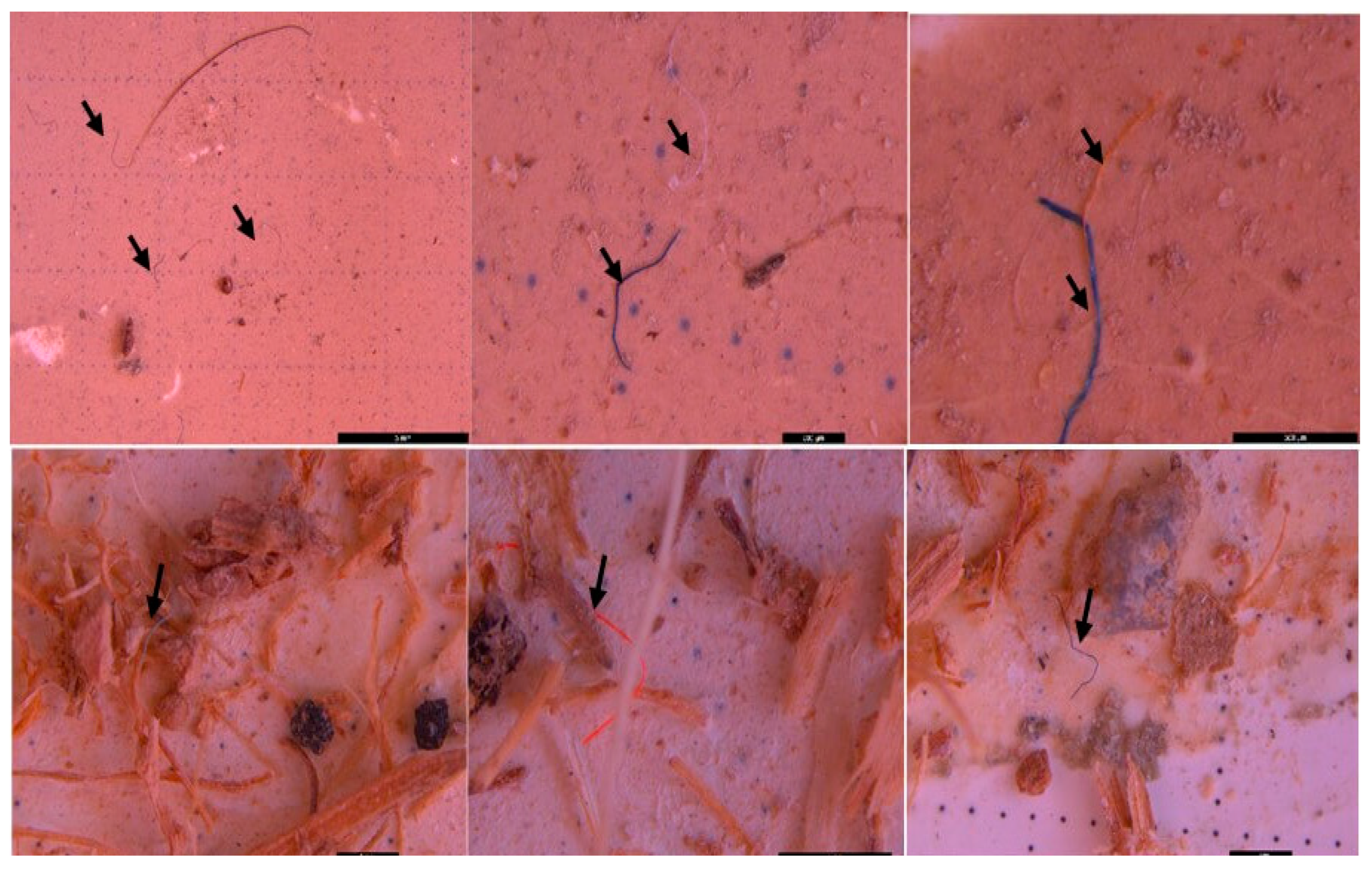
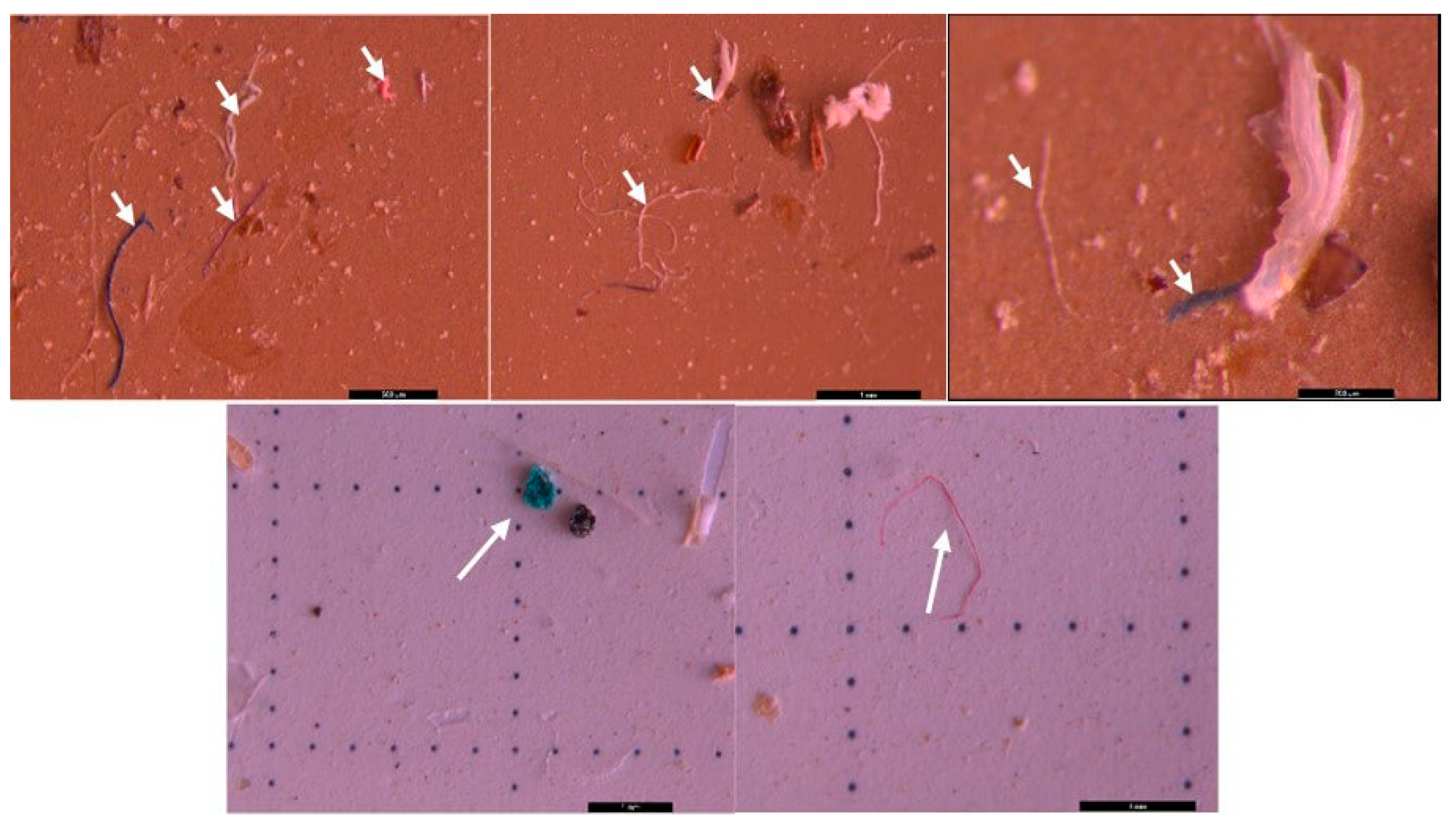
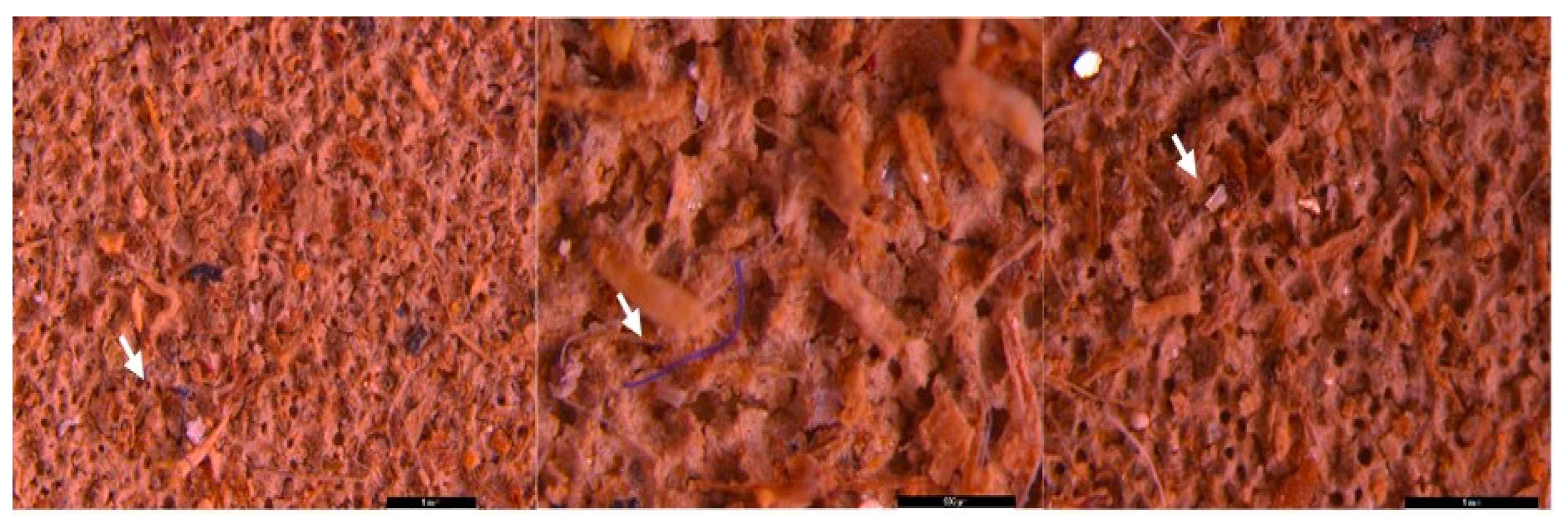
2.3.2. Microscopic Investigations of MPs

The second stage involved microscopic characterization. Classical microscopic analysis (Motic optical microscope, 10× and 40× objectives) (Motic, Germany) of the MPs samples highlighted particles suspected to be microplastics. In addition, a Leica M205FA stereomicroscope (Wetzlar, Germany) was used for the macro/microplastics observations. The presence and physical characteristics of the MPs (colors, shapes, and sizes) were acquired with Leica Application Suite V4.12 image software.
The SEM-scanning electron microscopy analysis (SEM Quanta FEG 250, Thermo Fisher Scientific, Waltham, MA, USA) was used to evaluate the size and morphological characteristics of the microplastics. All samples were analyzed in LoVac (low vacuum) mode. In this type of working mode, water vapors are pumped into the microscope chamber in order to preserve the samples. Additionally, the SEM investigations were carried out using an Everhart–Thornley Large Field Detector (LFD). This type of detector is ideal for general imaging due to the fact that it contains BSE (backscattered electrons) and SE (secondary electrons). All the filter membranes containing the investigated samples were cut into small square pieces with approximate sizes of 1 × 1 cm2. After that, the samples were mounted on stab holders which were previously covered with double-sided conductive adhesive carbon tape. All of the samples were analyzed under the same conditions with an electron acceleration voltage of 20.00 KV. No contrast agent was used during the analysis. The samples were not coated with any electrically conducting metals.

2.3.3. Methods for MPs Identification

The MPs identification was made using two complementary spectrometric techniques, Raman and FT-IR, using different available equipment. Because there was no polymers database available, for the identification of MPs spectra we used three reference polymers (those most frequently found in surface waters: PE CAS 9002-88-4, PP CAS 9003-07-0, and PS CAS 9003-53-6) or the literature data.
  • Raman analysis—Raman-HR-TEC-785 Spectrometer
The samples were analyzed on a Raman-HR-TEC-785 Spectrometer (StrellarNet Inc., Carlson Circle Tampa, FL, USA) equipped with the Raman Probe-785 featuring integrated optical fibers and a laser excitation system with a wavelength of 785 nm. The wavelength range is 200–2700 cm−1. The optical resolution is 4 cm−1. The diffraction grating is 1200 g/mm with gold coating. Data processing and obtaining spectra were carried out with the help of SpectraWIZ Software v5.33 and 6.32, SpectraWiz-ID, LabView 8-2, Spectroscopy Pro-tools v1.2.15.
2.
Raman analysis—NRS-7200 Raman Spectrometer
Polymer particles isolated on filter membranes were analyzed using the system NRS-7200 Raman Spectrometer B000461423 with a microscope (JASCO INTERNATIONAL CO., LTD., Tokyo, Japan). Information for the Raman spectrometer is as follows: resolution 0.7 cm−1, detector 4-Stage Peltier Cooled CCD Detector (UV-NIR range, 1024 × 255 pixel), spectral range: 5 to 8000 cm−1. General measurement information: exposure time 30 s; accumulation 10, 20; laser wavelengths 785 and 530 nm; laser power 5.6 and 56.6; objective lens 10×. The spectra were collected using JASCO Canvas Program.
3.
µRaman analysis—LabRam HR800 system
The µRaman analysis was performed for the samples filtered on gridded cellulose ester membrane after the separation process. The Raman studies of MPs samples were conducted at room temperature by confocal µRaman Spectroscopy using a LabRam HR800 system (Horiba, Kyoto, Japan). All the Raman spectra were generated within a 100–4000 cm−1 spectral range by exposing the specimens for ~200 s (in total, a 40 s/spectral window) to a 2 mW, 632 nm wavelength red excitation laser using a 50× long working distance objective. The signals emitted by the samples were dispersed onto a cooled CCD detector down to −70 °C, using a 600 lines/mm grating with a spectral resolution of 0.6 cm−1. All Raman spectra were collected using the LabSpec software v.5.
4.
FT-IR—Cary 630 FT-IR Spectrophotometer
The infrared spectra were recorded with a Cary 630 FT-IR Spectrophotometer (Agilent Technologies, Santa Carla, CA, USA) based on the pellets’ formation with KBr (2 mg sample + 200 mg KBr, pelletized with a hydraulic press of 7–9 tons, vacuum 2 min) in the range of 400–4000 cm−1. Standard spectra were obtained for polyethylene and polystyrene using MicroLab Pharma Software v.5.6.
5.
ATR—FTIR measurements—Perkin—Elmer Spectrum Two IR spectrometer
The ATR—FTIR measurements of the samples were conducted under ambient conditions using a Perkin—Elmer Spectrum (v.10.5.1) Two IR spectrometer (Spectrum TWO DTGS 102,767 series). All spectra were recorded in the wavenumber range between 400 and 4000 cm−1 at room temperature using a DTGS detector. Each ATR—FTIR spectrum is the average over 10 scans, using air as reference, and 2 cm−1 as the nominal spectral resolution (PerkinElmer, Shelton, CT, USA).

3. Results and Discussion

3.1. Characterization of Floating Plastics Particles

In accordance with the specialized literature [45] we noticed that most of the plastics collected in the field, analyzed visually, are included in the group of mesoplastics < macroplastics < large microplastics (Table 1). No quantitative method was applied due to the short execution time. Table 1, referring to field data, includes the visual characterization of floating plastics (>5 mm) and other wastes (found in the established perimeter or in the washed sediment), in order to reveal the source of MPs.
The visual analysis of the filtered samples highlights the presence of particles of various sizes, possibly MPs (Figure S3). In all the analyzed samples, fragments of different colors (red, blue, and white), fibers, and spheres of polystyrene-type foam were highlighted. The most visible particles were highlighted in the cases of sediments determined on the 250 and 500 µm sieves. MPs less than 5 mm, such as fragments and spheres, were cleaned with ethyl alcohol and distilled water to remove impurities for the SEM and Raman analyses.
Depending on the type, the MPs exhibited regulated and unregulated shapes such as pellets, fragments, fibers, foam, and spheres. Fragment and foam types were frequently observed in the collected samples. Regarding coloration, the MPs varied as follows: white, transparent, black, red, brown, green, gray, and blue. The most prevalent were the white foam spheres, which are suspected to be PS.
In the wastewater influent from the local WWTP, a visual abundance of MPs particles <5 mm was observed (Figure S4). Consequently, the urban wastewater discharges contain polymers that reached into the aquatic environment. The polymer contamination depended on the retention capacity of the wastewater treatment processes. Some studies reported the presence of MPs in WWTP influents and effluents, with removal rates ranging from 20% to 90%. The size of the MPs ranged from 1 µm to 2000 µm and appeared in various forms (mainly fibers and fragments) and colors (predominantly white, blue, green, black, red, yellow, and transparent). Similar results were also reported by other studies [49].
These MPs were identified as PE, PET, PS, PVC, Polyamide, and Polycarbonate [50].

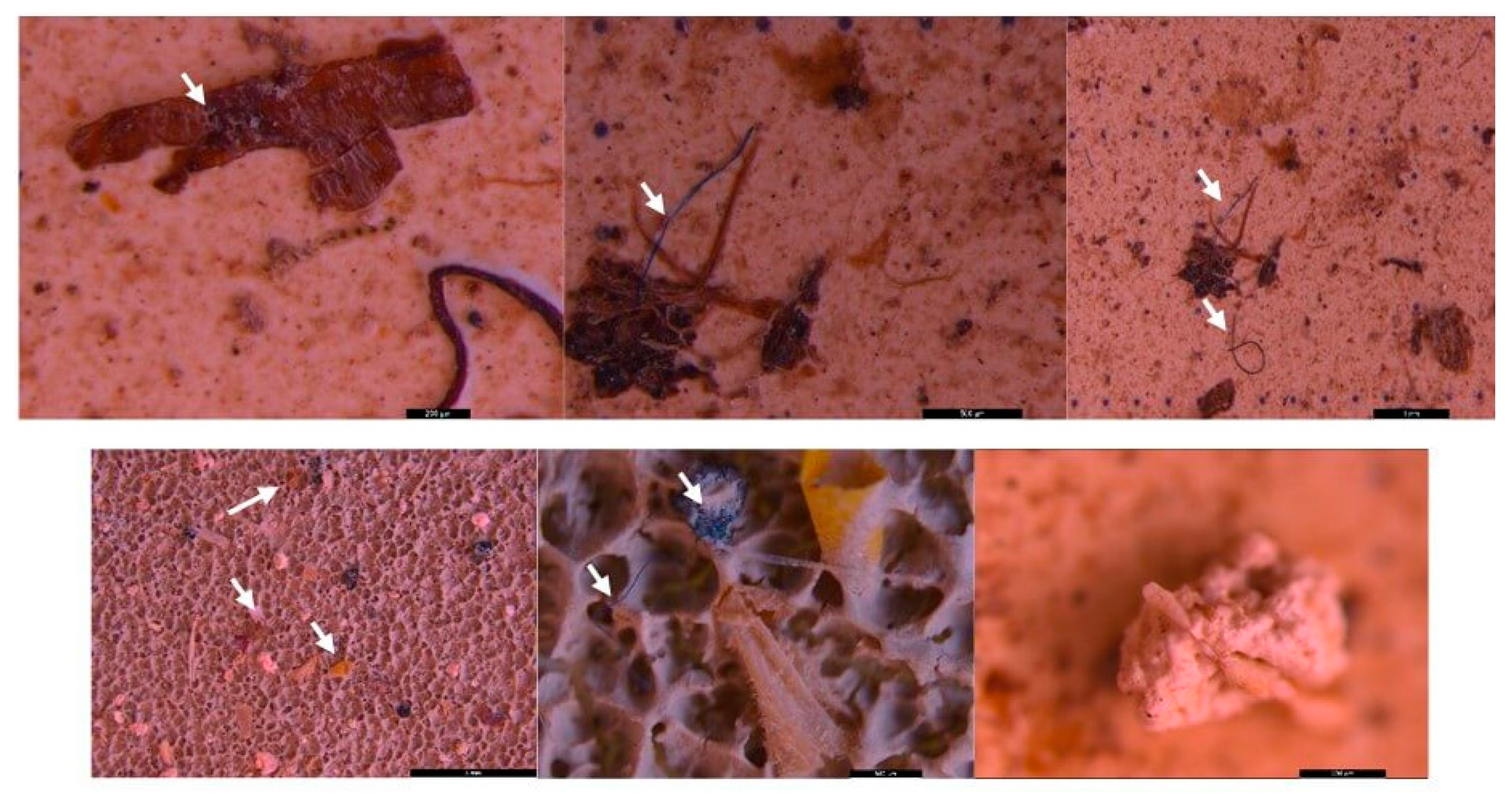
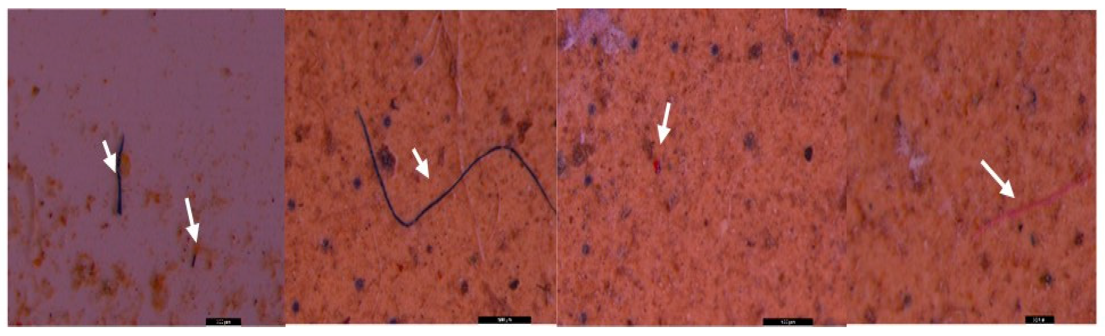
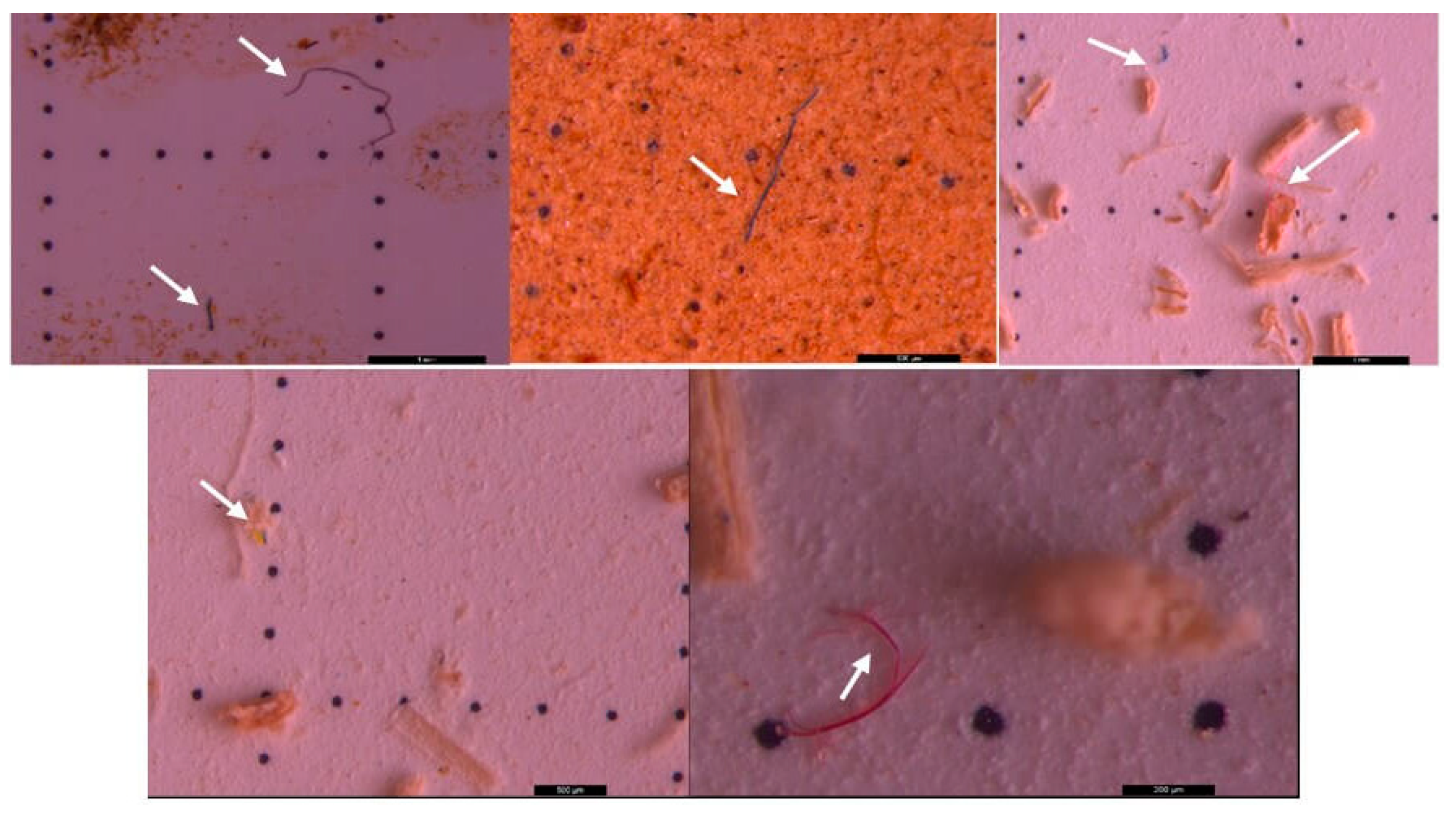
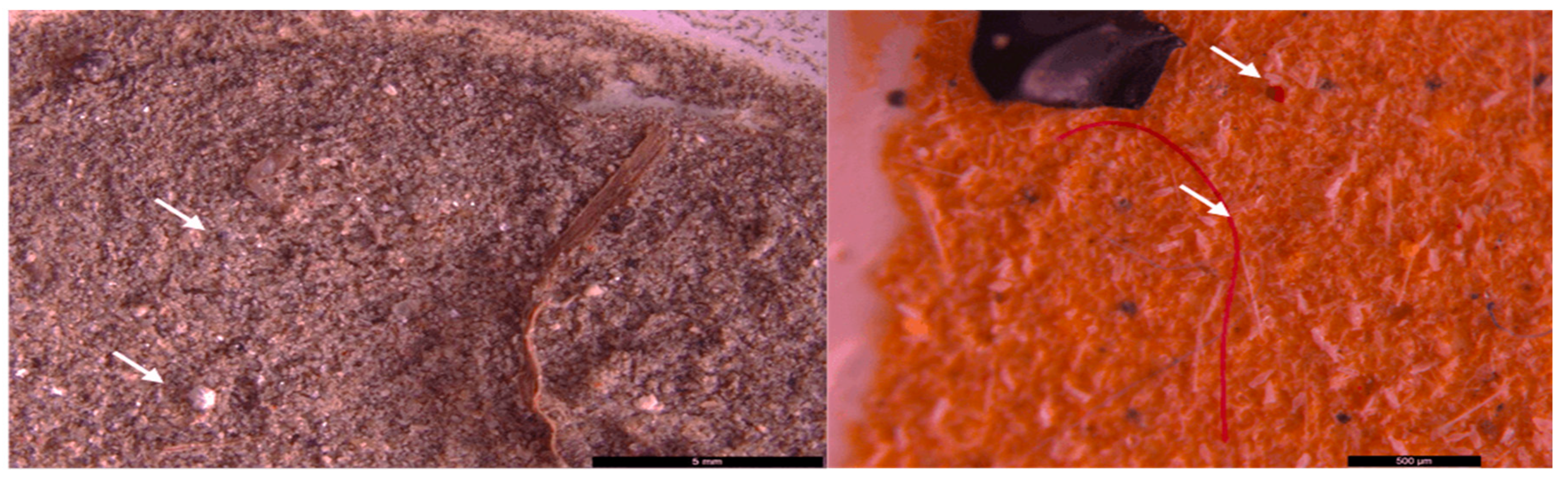
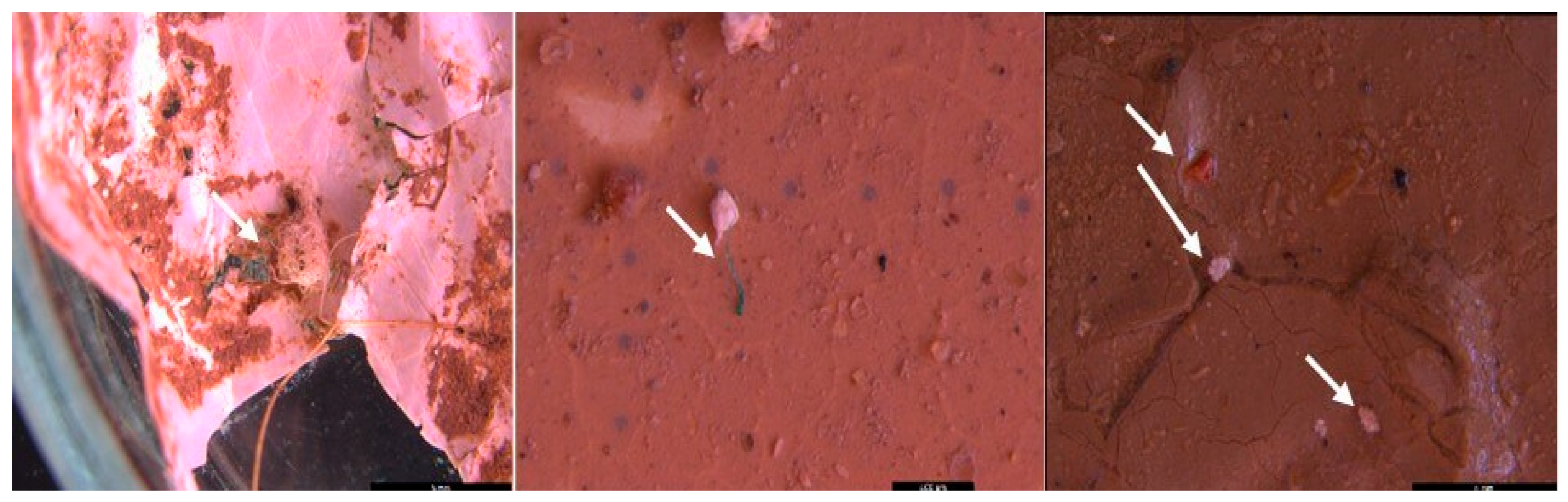
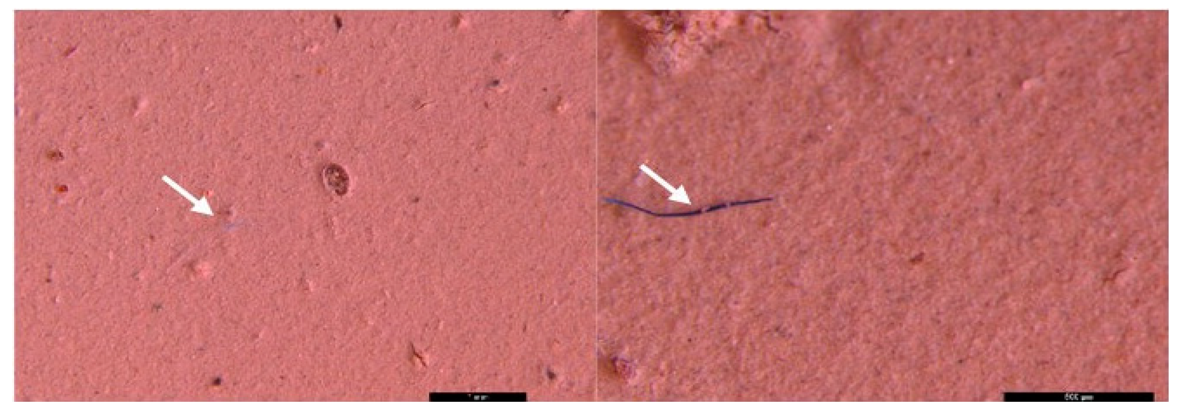
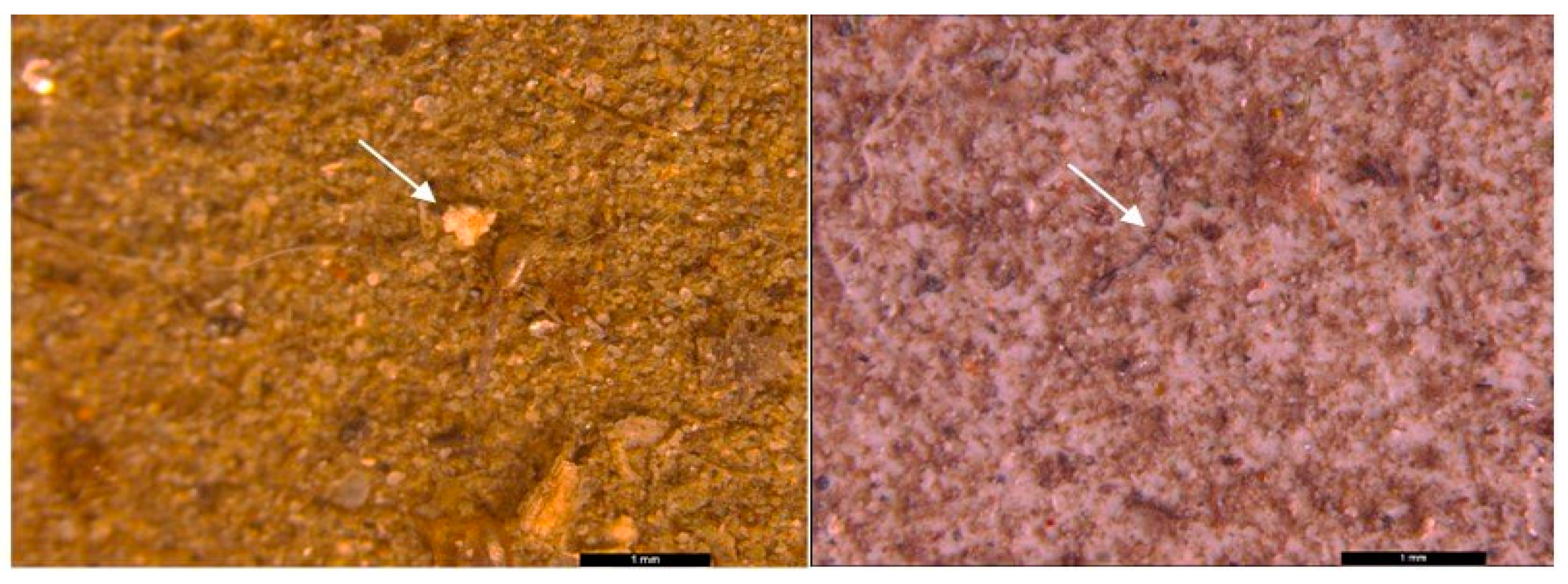
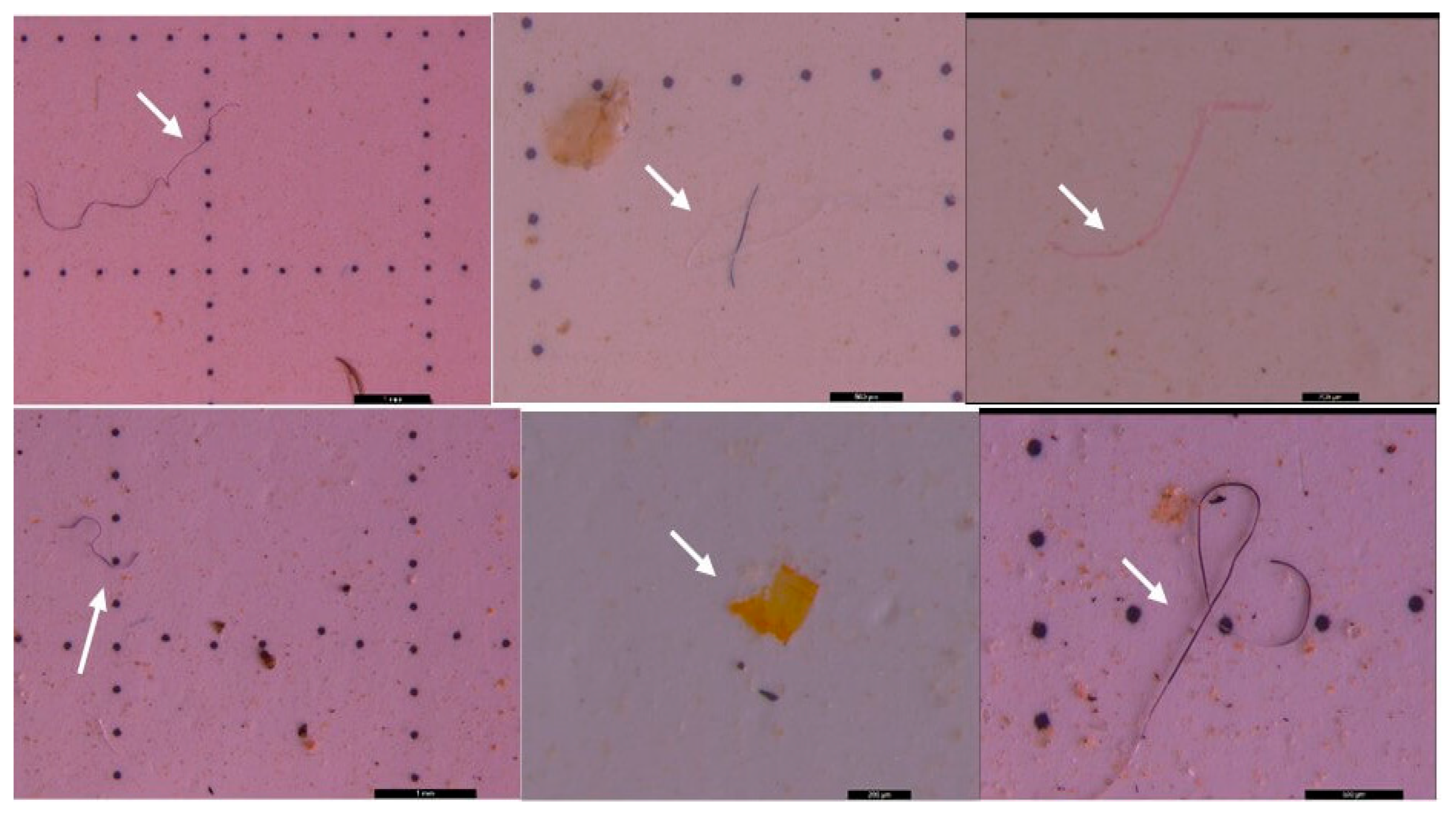
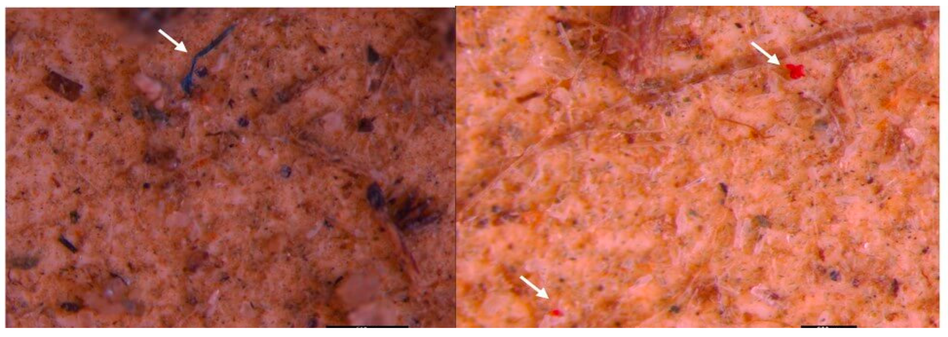
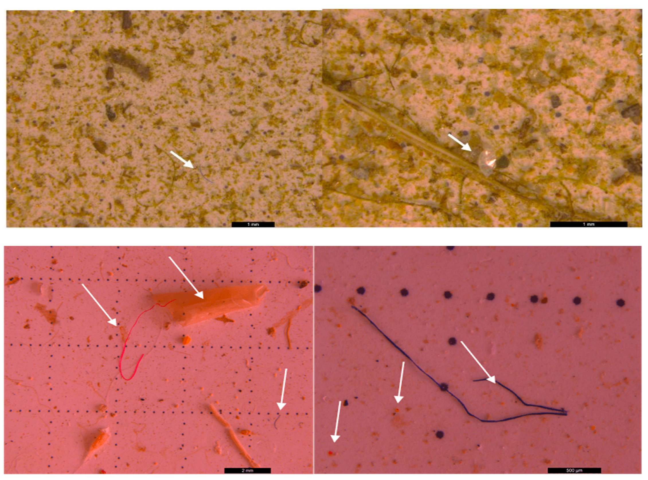
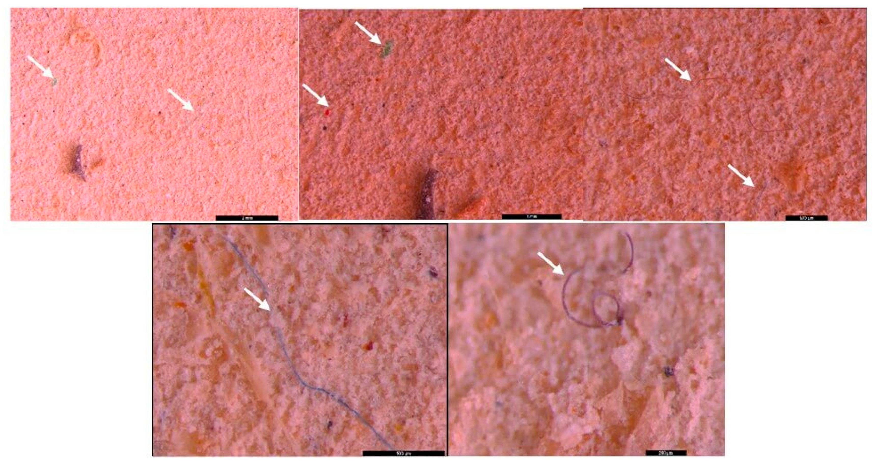
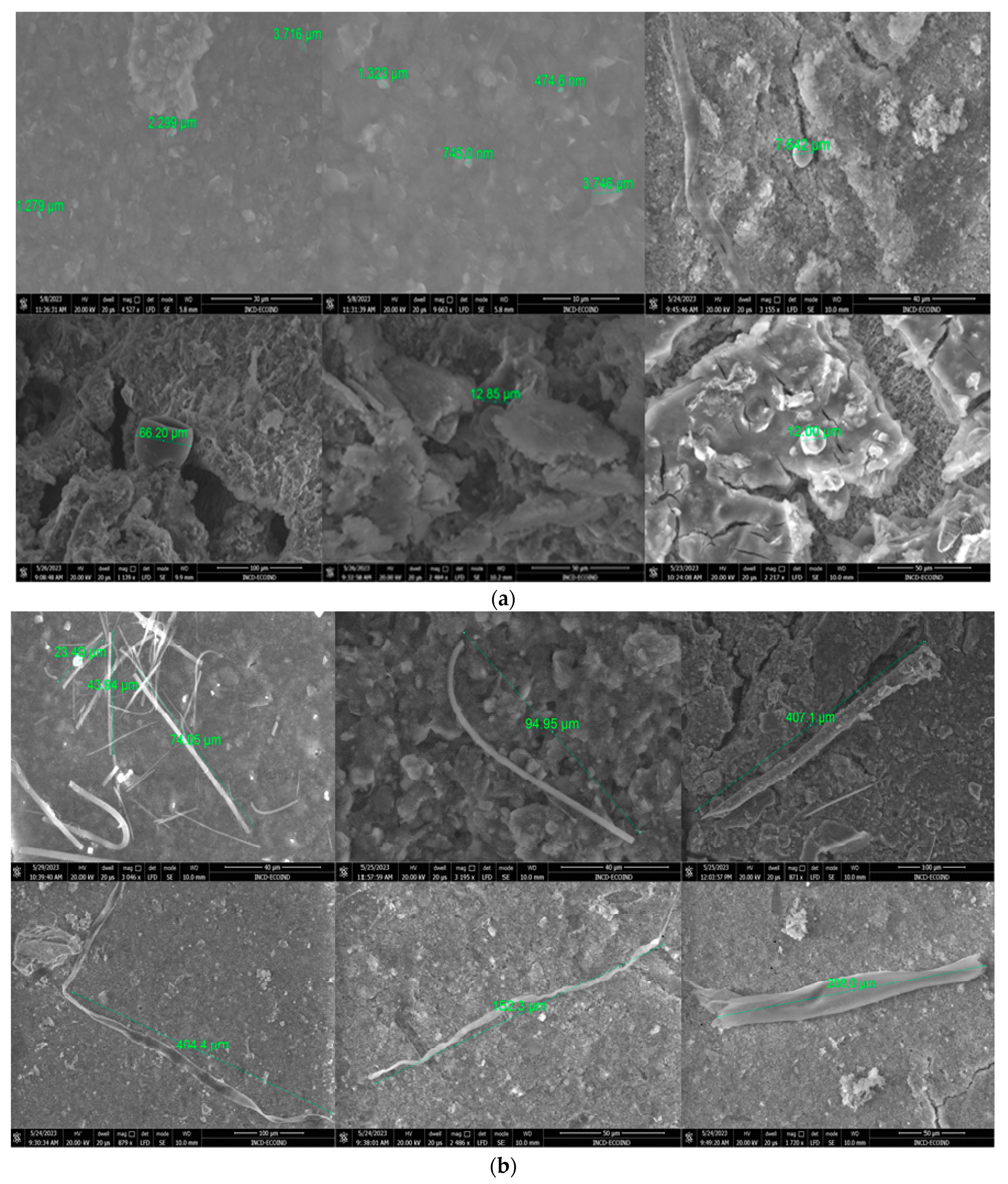
3.2. Microscopic Analysis of Separated MPs

While using the optical microscope (10×–40× objective), particles suspected to be MPs in the form of fragments and fibers were observed. It was found that the polymers are integrated in the aquatic system, attached to organic waste or filamentous algae, and were easily confused with the carcasses/remains of organisms (especially in the case of the transparent fragments) (Figure 2). Therefore, their characterization and identification require stages of organic matter removal and separation of the polymers.
The laboratory experiments revealed that oxidation with 30% H2O2 completely destroyed the organic matter. The applied method was robust and suitable for large MPs particles. Some tests performed on the reference MPs highlighted the fact that the particles can be separated but were no longer found in the same amounts at the end of the analysis because some were lost during the transfer stages, a fact also confirmed by the literature [51]. A better recovery was observed in the case of direct transfer to the filter membrane without using another intermediate glassware. Another interference was caused by NaCl crystals, which can be eliminated by successive washings with distilled water. When filtering via the filter membrane, issues arise with detritus and residues of oxidized matter that make the visibility of transparent MPs particles confusing and difficult. Through the classic microscopy method, the MPs particles less than 1 mm were separated and subsequently microscopically characterized and identified.
In all analyzed samples (sediment, surface water, and wastewater) the stereomicroscopic analysis (Leica M205FA stereomicroscope) revealed the presence of MPs in different shapes, colors, and sizes (Figure 3, Figure 4, Figure 5, Figure 6, Figure 7, Figure 8, Figure 9, Figure 10, Figure 11, Figure 12, Figure 13, Figure 14, Figure 15, Figure 16, Figure 17 and Figure 18). The most common types of MPs were the fibers (e.g., Figure 3), which appeared in a range of colors including white, blue, purple, pink, orange, and black. These fibers measured from 100 µm to over 5 mm and were more abundant in the sediment samples. These fibers, with their low densities, were associated with materials such as polyester, nylon, rayon, or polypropylene. The prevalence of the fibers aligns with observations made by other authors [52] using the stereomicroscope, who found similar fibers in sizes less than 2 mm from synthetic textiles as possible sources. It is supposed that the fibers are more dangerous for aquatic animals because they are more difficult to be eliminate from digestive tracts as compared to the fragments or spherical MPs, which leads to prolonged exposure [53].
The second type of MPs was fragments of hard polymers or foils in different colors and shapes, which result from the environmental degradation of large pieces of plastic (e.g., Figure 4, Figure 7, and Figure 14). Transparent or opaque, red, yellow, blue, pink, or green fragments were identified. Their sizes varied between <100 µm and 2 mm with a higher density in the sediment samples.
Another frequently encountered category in the samples taken from the Somesul Mic River consisted of fragments and spheres of PS foam (e.g., Figure 6 and Figure 7), which were generally white or gray-white, making them very easy to notice. PS has a low density and was frequently observed even in unconcentrated surface water as well as floating on the surface of the water. The prevalence of PS is likely linked to uncontrolled construction waste storage.
The sizes of the particles were determined microscopically and some of them correspond to the physical characteristics of PS, which were between 500 µm, 1 mm, and ≥3 mm, but there is a possibility of the presence of smaller fragments < 500 µm which were the result of the pressure of biological processes, sunlight, or purification processes. The results are comparable with the findings in the national literature, which indicate that PP, PS, and PE are the most frequently encountered polymers in water bodies such as the Danube River and the Black Sea. Their low density allows them to float and to be easily collected from the surface water [26].
The microscopic analysis highlighted the fact that most of the particles were identified as being polymeric in nature (plastic); they were large MPs with sizes that ranged between 1 mm and ≤5 mm (fibers, fragments, foam, and spheres), as well as small MPs ≤1000 µm, such as the fragments.
The literature confirms that 90% of MPs are represented by fibers and, in a smaller proportion, by fragments, clumps, and spheres [26]. In this case, the fibers are most easily identified based on their specific forms and colors. The fragments are more challenging to identify due to their diverse and unregulated shapes, as well as their transparency.
The types and shapes of the observed MPs in the sediment and surface water were also identified in the wastewater effluents; notably, PS foam was poorly represented. In this case, the most abundant types were the fragments and fibers.
We cannot ascertain a significant difference in the MPs load in terms of the sampling points, because all the samples showed the omnipresence of MPs. However, it can be seen that the Cluj–Napoca WWTP can be a source of small MPs (Figure 18), because the large ones are retained in the mechanical stage and in the activated sludge.
The abundance of MPs of various sizes and shapes leads us to the hypothesis that the most important source of the water body’s contamination is the improperly stored waste on the banks of the river, a phenomenon also observed on the field. The washing of the banks by the river and the environmental conditions inevitably contribute to the destruction and degradation of macroplastics into MPs and to their being carried along the body of water until they are discharged. Sediments represent storage reservoirs for MPs, as well as for numerous chemical pollutants.
Due to the fact that the MPs could be separated based on their density in NaCl, it can be seen that the microscopically observed MPs can be part of the class of low-density polymers such as polyethylene, polypropylenes, polystyrene, ethylene-vinyl acetates, and polyamides.
The analysis of the unused sterile-filter control membranes used in the takeover of the MPs for microscopic analysis did not reveal the presence of impurities or types of MPs that would contribute to or interfere with their identification in the environmental samples.
The obstacle of the microscopic method was the identification of transparent fragments less than 100 µm, which are difficult to observe and characterize. The literature estimates that 20–70% of these fragments can be identified using other, more advanced methods [54]. The density of the sample sediment on the filter membrane and the presence of impurities that cannot be eliminated by digestion (such as insect carcasses, natural fibers, etc.) were impediments during the microscopic observations.
SEM microscopic analysis revealed the morphological surface structure of the MPs. Compared with the classical microscopy method, the SEM technique revealed the small MPs particles ranging from less than 1 µm to 500 µm (Figure 19). Additionally, a better morphological characterization of the MPs could be highlighted using this method. The surfaces of the fragmented polymer materials were irregular. The fibers have smooth surfaces and linear shapes, while the foam exhibits rounder shapes. The sizes of the MPs influence their bioavailability to organisms: the smaller they are, the more negative their effects can be [55].
Additionally, it was possible to highlight the structure of some aging particles larger than 1 mm (Figures S5 and S6). Other particles were observed in the wastewater without being subjected to the oxidizing digestion treatment. They have the shape of elongated transparent films with sizes greater than 500 µm, while others are fragments of ≤50 µm (Figure S6).

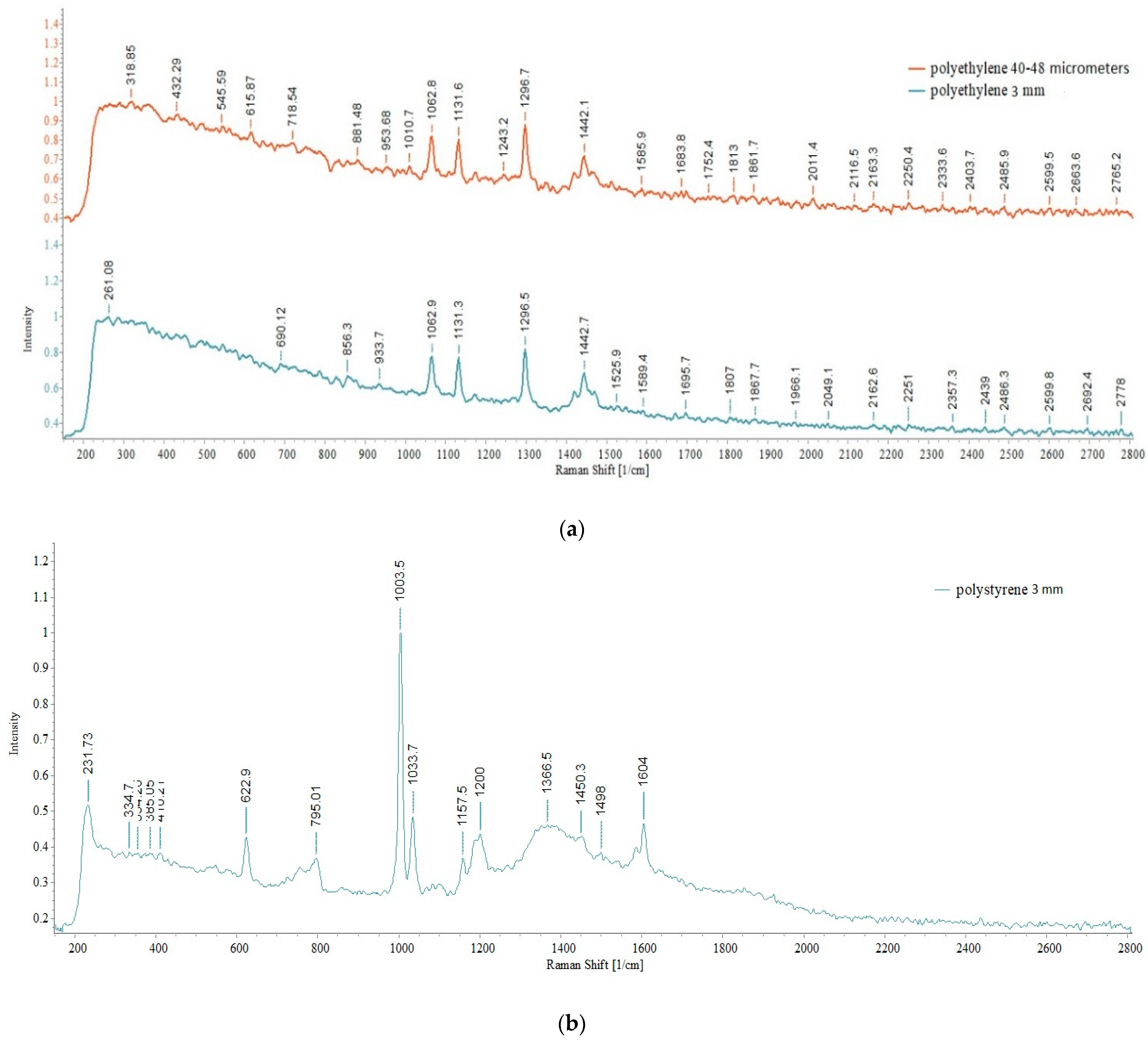
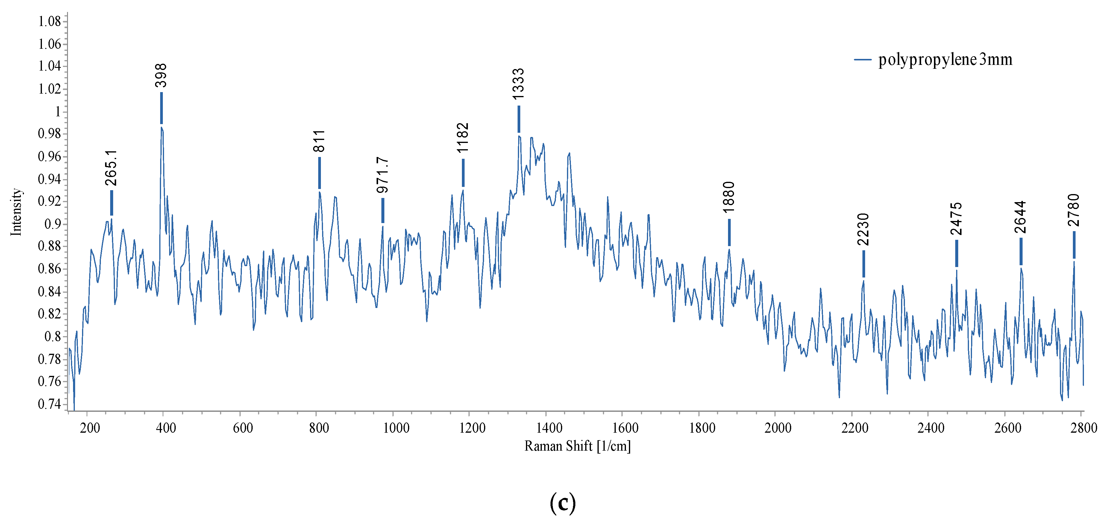
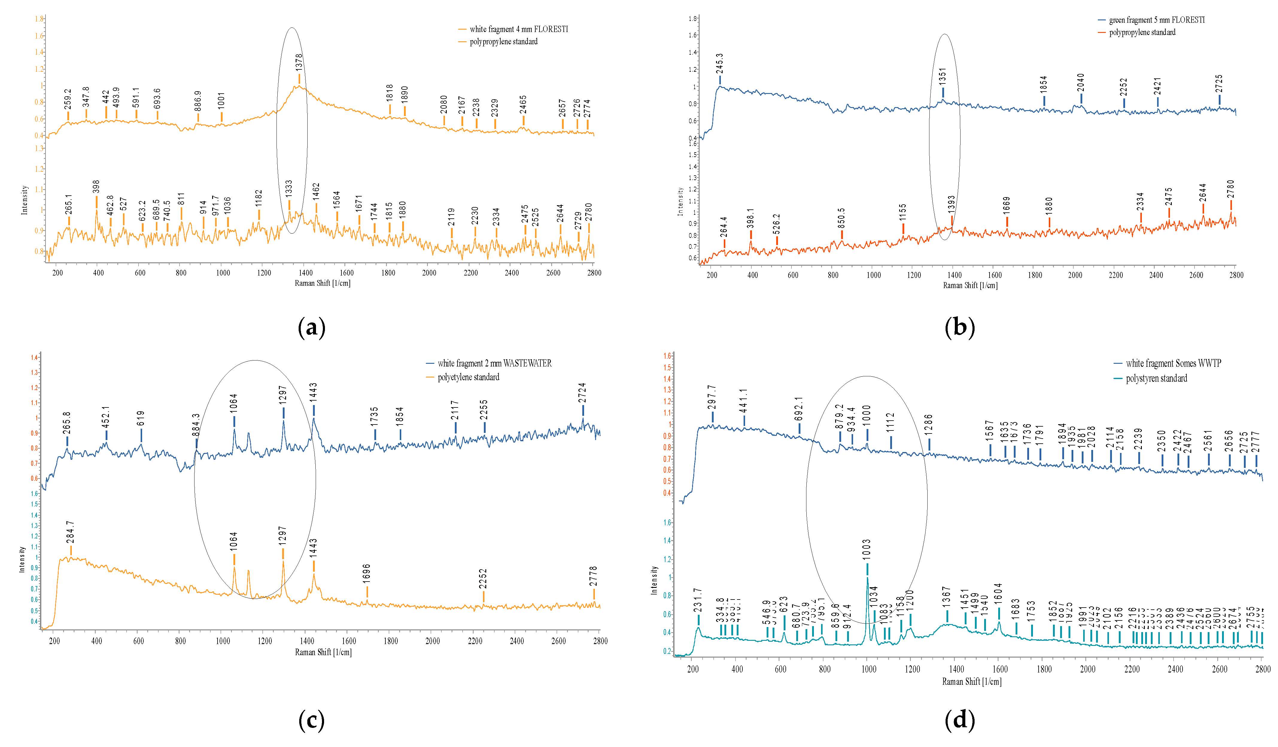
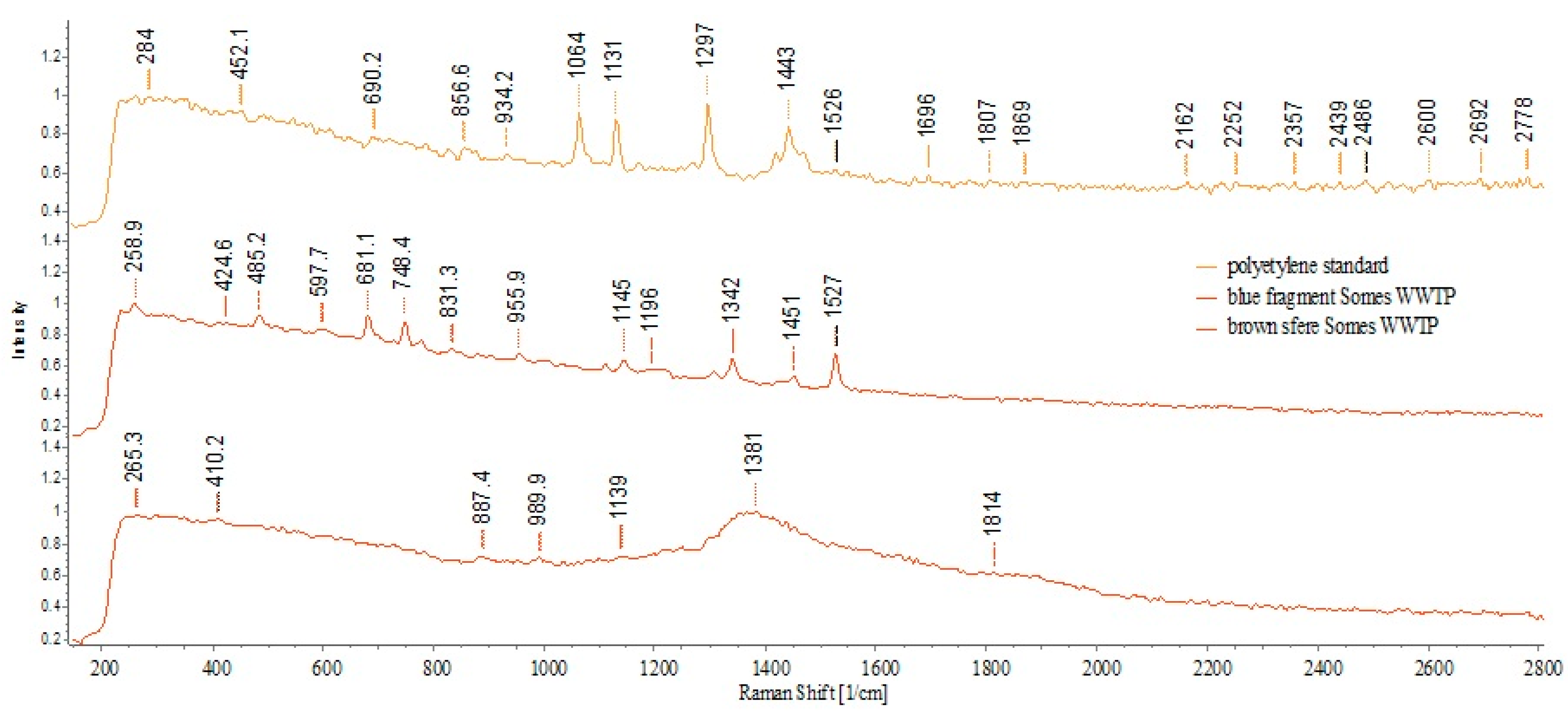
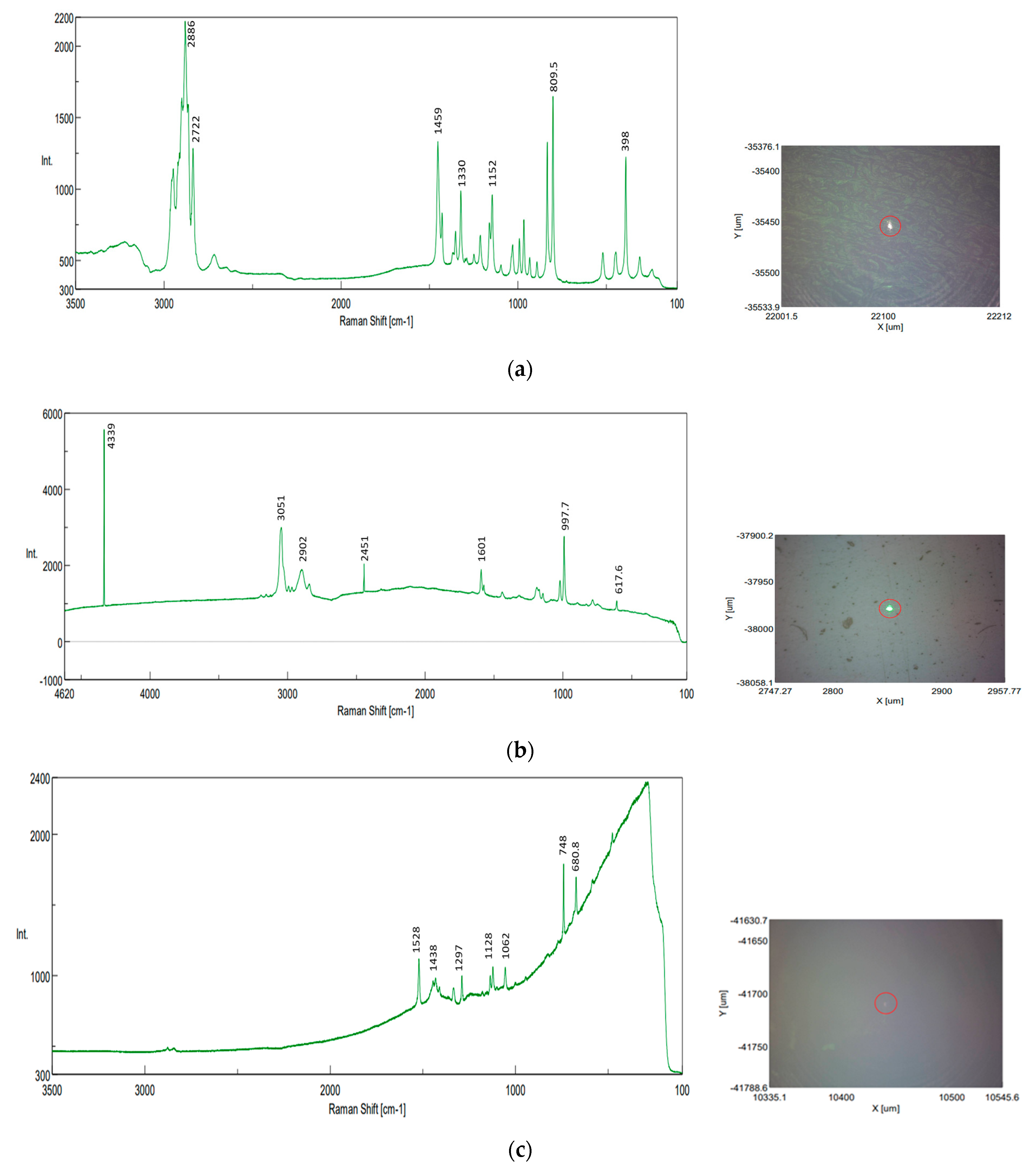
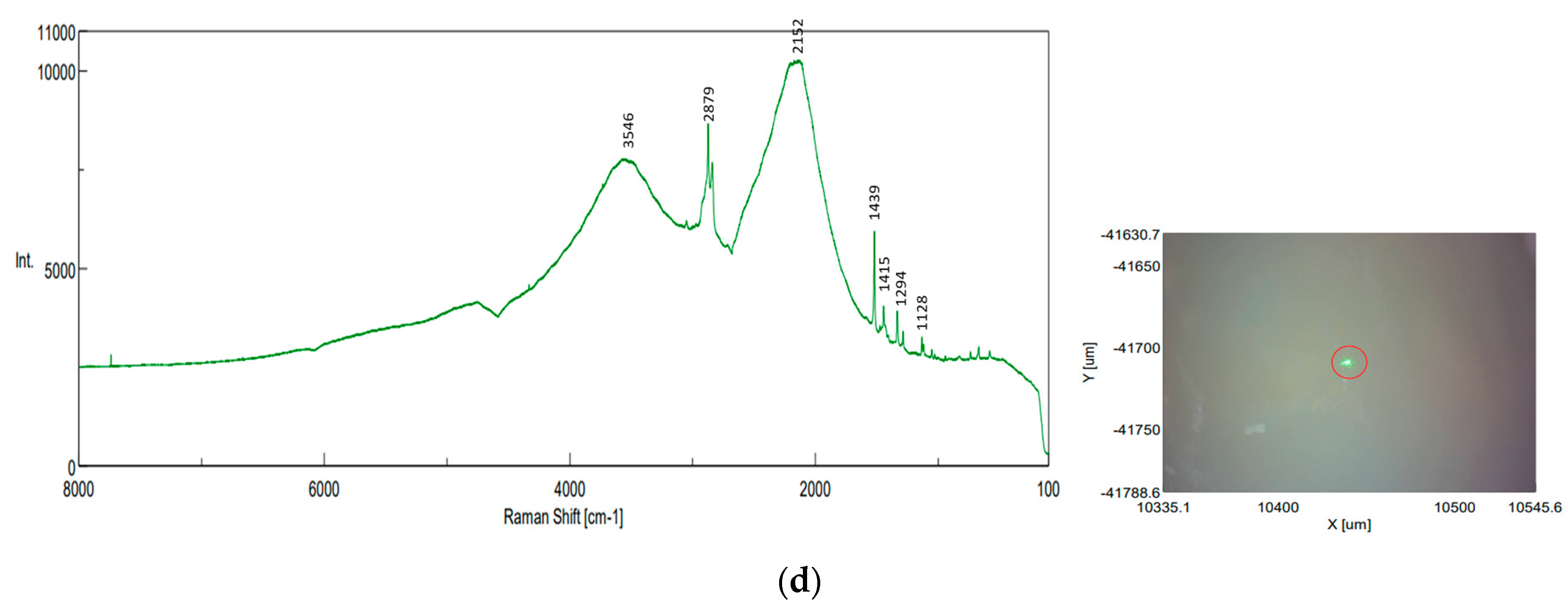
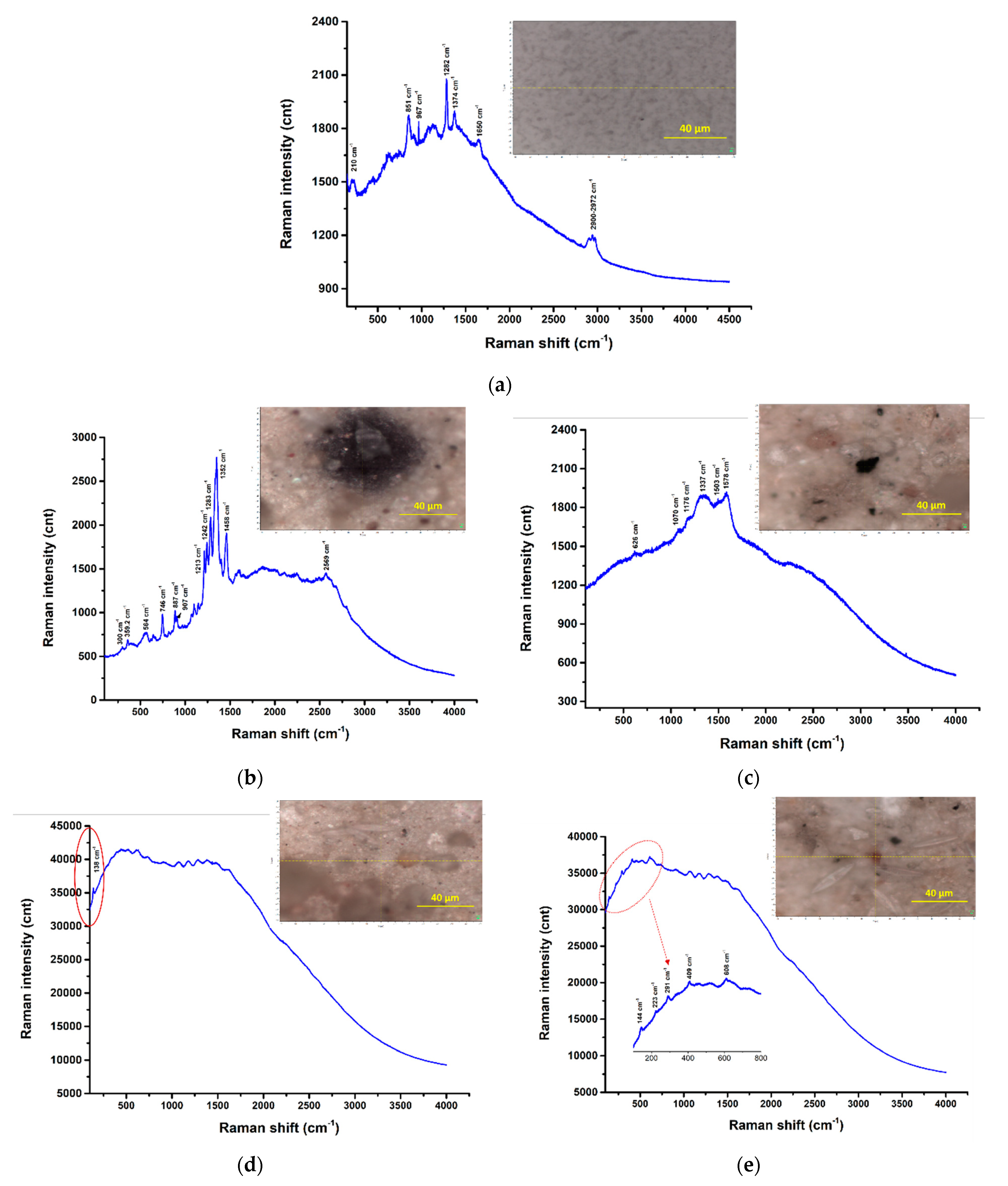
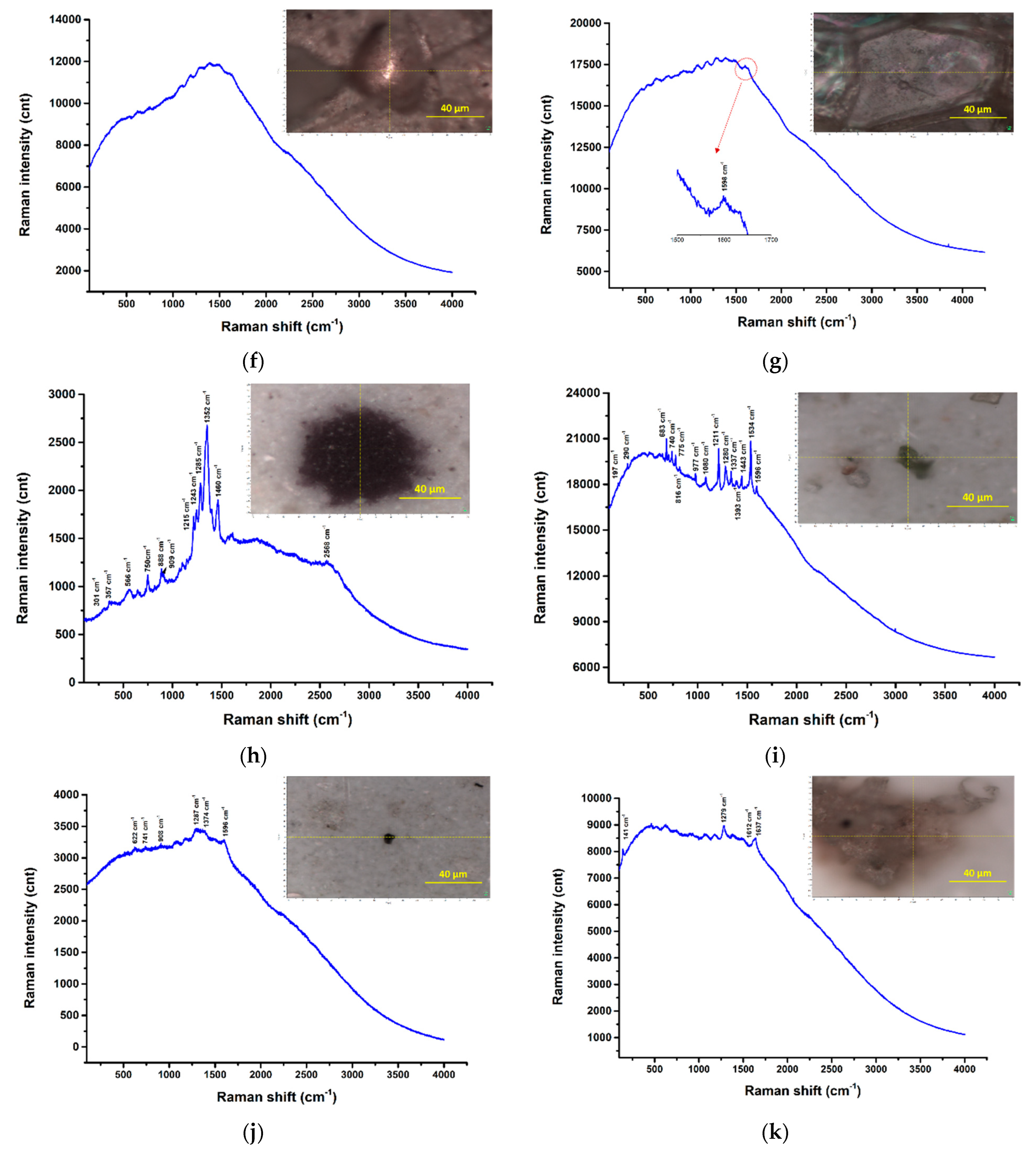
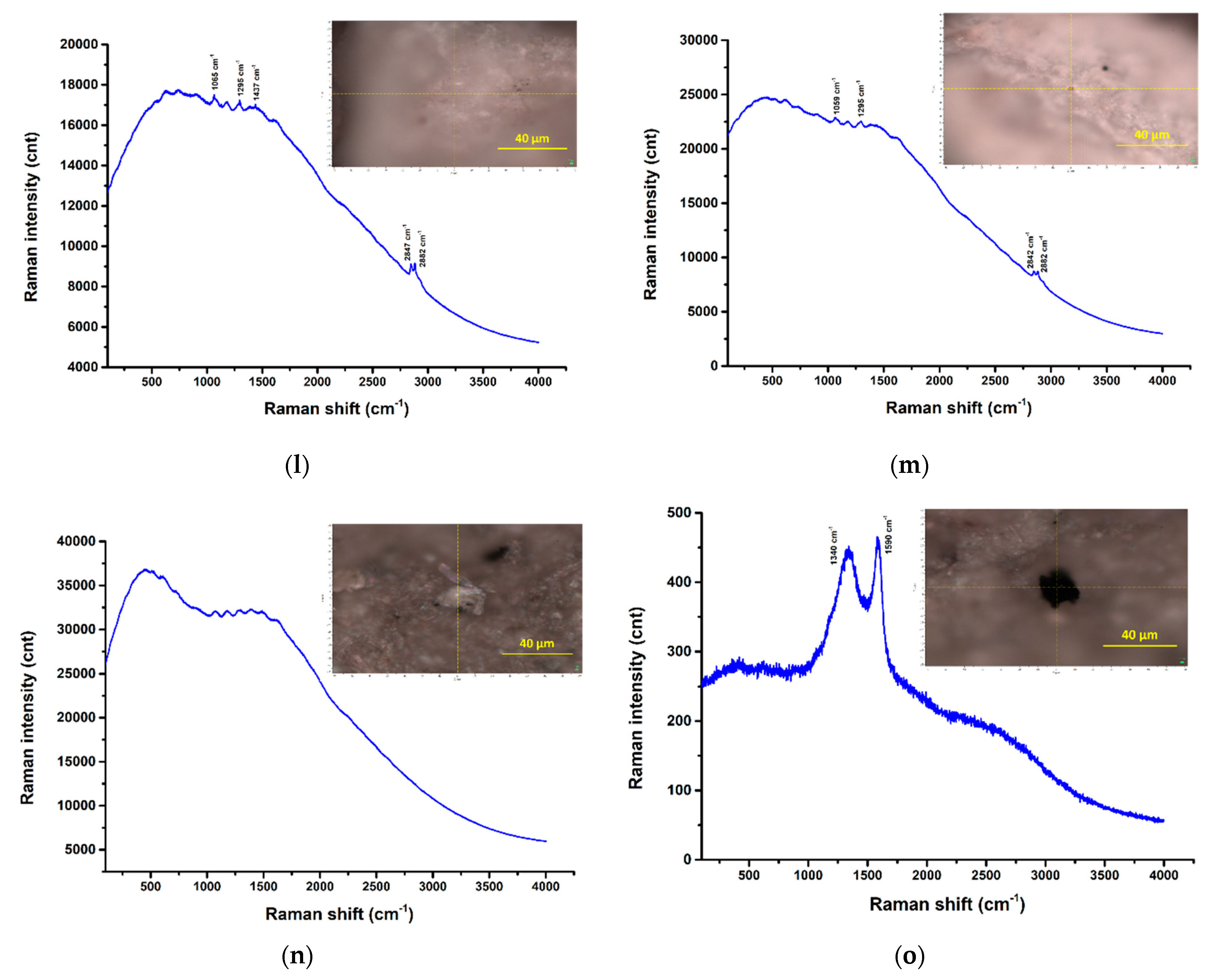
3.3. Raman Investigation

The obtained results of the Raman-HR-TEC-785 applied on large particles (>500 µm) and based on the reference spectra of PE, PS, and PP (Figure 20) showed the following estimation of identifications: PP (white and green fragments 4–5 mm) in the sediment UP Floresti (Figure 21a,b); PE (white fragment, 2 mm) in the wastewater influent of Cluj-Napoca WWTP (Figure 21c) and in the sediment of UP Cluj-Napoca WWTP (colorless fragments 1, 3, and 4 mm (Figure 21e), and brown sphere 2 mm (Figure 22)). The obtained spectra are comparable to those obtained by [56]. The identification of fragments smaller than 500 µm was not possible (Figure 21d).
This analysis has some limitations: (i) the presence of organic or inorganic impurities can interfere; (ii) an obscure ambient environment must be ensured because light induces fluorescence; (iii) the color of the MPs, additives, and their transparency can interfere with obtaining of spectra; (iv) regarding the size of the MPs, the spectra were obtained for particle sizes >1 mm while the particles <1 mm can be destroyed by the laser light or cannot emit sufficient signals to obtain spectra. Even so, the Raman technique using the Raman-HR-TEC-785 Spectrometer allowed for the identification of PE and PP polymers using particles sizes of ≥1 mm, taking in to consideration the standard spectra (Figure 20a–c). Because the analyses feature limitations and interferences, the results of identification are not clear.
The NRS-7200 Raman Spectrometer obtained good results that confirmed the presence of PP, PE, PS, and, additionally, polycarbonate (PC) in sediment samples (Figure 23). Even so, the method encountered challenges in identifying the MPs trapped in the sediments or organic matter residues in filter membranes.
The size of the MPs and the absence of databases for polymer spectra also contribute to difficulties in analysis and interpretation. According to the literature, the ranges of Raman vibration frequencies for the main common plastic polymers are as follows: PE is in the range 1062–2883 cm−1, PS is in the range of 621–3054 cm−1, and PP is in the ranges of 809–1458 cm−1, 2883–2952 cm−1 [1]. The obtained spectra revealed the following peaks: CH starting with 2886 cm−1 to 809 cm−1 characteristic of PP; 997, 1601, 2451, 2902, and 3051 cm−1 for PS; 680 cm−1 to 1528 cm−1 for polycarbonate; and 1128, 1439, and 2879 for PE, almost similar to [56].
The µRaman study using the LabRam HR800 system was performed in several areas of the MPs samples, using the integrated optical microscope for identification. Some representative spectra for the investigated samples (filtered surface water) are shown in Figure 24b–o. Only a few investigated regions showed clear Raman bands; the others only showed significant fluorescence and a series of broad bands of low intensity that can be attributed to potential organic degradation which could have been induced also by laser exposure. Figure 24a presents the Raman signature exhibited by the filter paper used in sample preparation.
As can be seen, the Raman signature of the DW Cluj-Napoca WWTP 200 µm sample (Figure 24l,m) consists of the following Raman bands: 2882 cm−1, 2849 cm−1, 1441 cm−1, 1294 cm−1, which can clearly be assigned to PE. These are the only Raman spectra from the Horiba LabRam-based experiments that were clearly attributed to the detection of MPs.
There are regions where multi-peak Raman profiles were detected with clear/sharp bands, but these were extremely difficult, unclear assignments, such as the ones shown in Figure 24b (UP Cluj-Napoca WWTP 20 µm) and Figure 24h,i (DW Cluj-Napoca WWTP 20 µm). In all of these cases, some of the bands, e.g., 1351 cm−1, 1462 cm−1, can be attributed to PP, and thus the presence of this polymer can be confirmed, even if these bands are not the most intense/main for this plastic. It should be noted that additives and/or dyes or pigments are usually used in these plastics, and their presences can cover the main bands or even the entire specific set of polymer bands. However, the other bands, except those assigned to PP, could not be identified. On the other hand, for some regions of the UP Cluj-Napoca WWTP 20 µm sample (Figure 24d,e), the detected bands were attributed to pigment residues such as TiO2 (anatase phase), white pigment; and α-Fe2O3/FeO(OH)nH2O, red pigment, respectively, which were probably used to color some polymers (not detected in these cases).
The Raman spectra shown in Figure 24c,j and o reveal the presence of D and G bands at approximately 1137 cm−1 and 1578 cm−1, respectively, which are specific for carbonaceous materials. This may either confirm the presence of C-forms in the wastewater samples or may be the result of the real-time degradation of the organic components in the samples as a result of their exposure to the laser beam.
Raman spectroscopy was commonly used for MPs detection in water, sediment, and biota systems, as evidenced in the literature [6,54]. However, its utility is still in its early stages of development regarding its ability to identify small MPs particles, particularly those less than 500 µm [1,55]. The configuration of equipment has a considerable impact on the analysis outcomes, especially in relation to the laser excitation wavelength employed. The most frequently utilized laser wavelengths were 532 nm, 632 nm, and 785 nm; the latter wavelengths were also used in our study. The main problem with 532 nm and 632 nm laser sources is that there are some analysts or impurities with fluorescence emission that interfere with the detection of MPs particles. The presence of noise background and fluorescence is characteristic of the existence of organic and inorganic materials [56]. As can be seen, all the Raman spectra shown in Figure 24 show significant fluorescence signal, which may have covered the signal of possible microplastic materials present in the analyzed regions. Also, the choice of the acquisition times and laser powers could increase the signal intensity and reduce the noise ratio.
The results of spectroscopic analysis can also be significantly influenced by the preparation of sample before analysis. The recorded Raman signals, potentially originating from the plastics present in the sample are not easily identifiable based on existing literature data; some suggestions were offered, but the peaks obtained do not perfectly fit the different plastic materials common in such environments [1]; in any case, it must be considered that this behavior can be justified by the probable presence of different pigments or contaminants. According to existing literature, the primary limitations of Raman spectroscopy are the fluorescent compounds (such as pigments, degradation compounds, organic residues) as well as the size of MPs [59]. Other sources of interference are linked to the reagents used in MPs separation, such as H2O2, FeSO4·7H2O and NaCl [33] or even the specific type of filter membrane. Filter membranes based on cellulose esters appear to introduce interference in the Raman detection of plastic polymers. Additionally, factors like substrate thickness and the distribution of the particles on the filter can compromise the accuracy of Raman detection [60].
According to the literature, the utilization of 30%H2O2 in the digestion process can lead to reductions in Raman peaks of certain compounds such as polyamide or color changes [61].

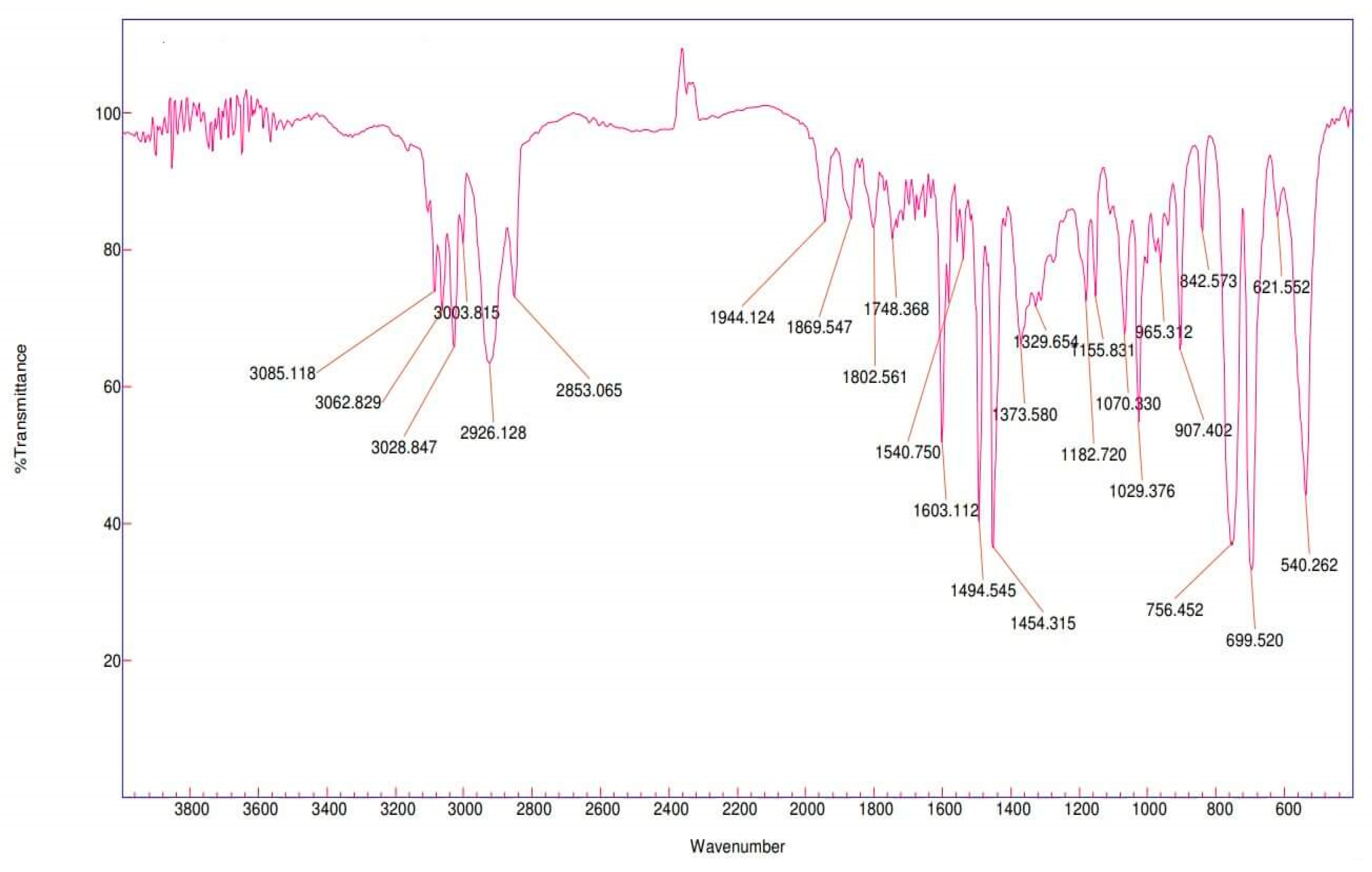
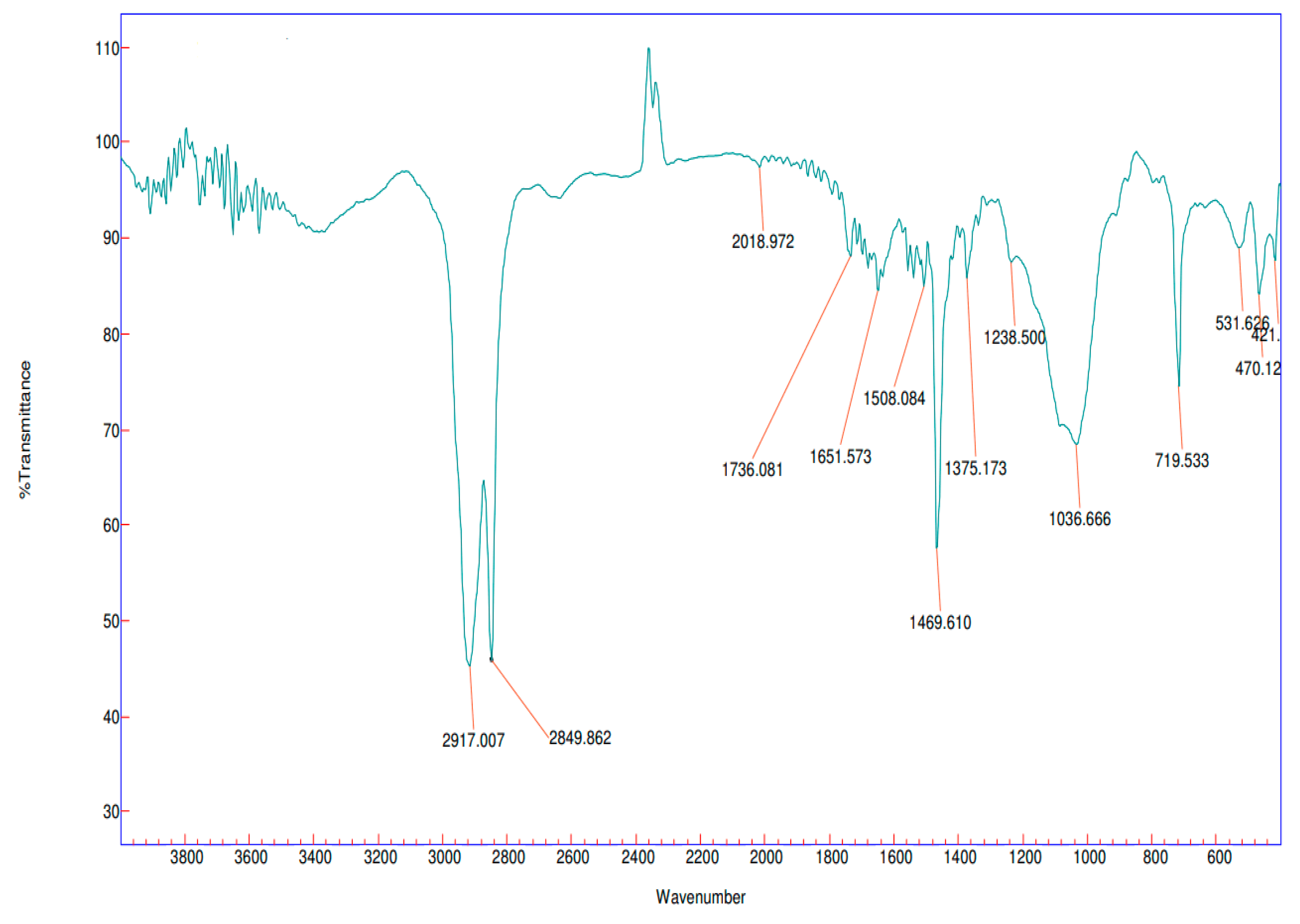
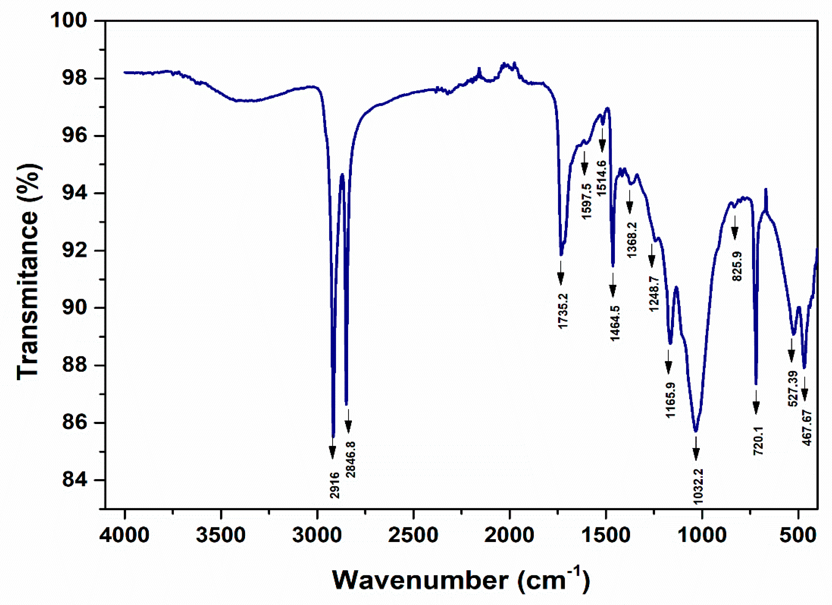
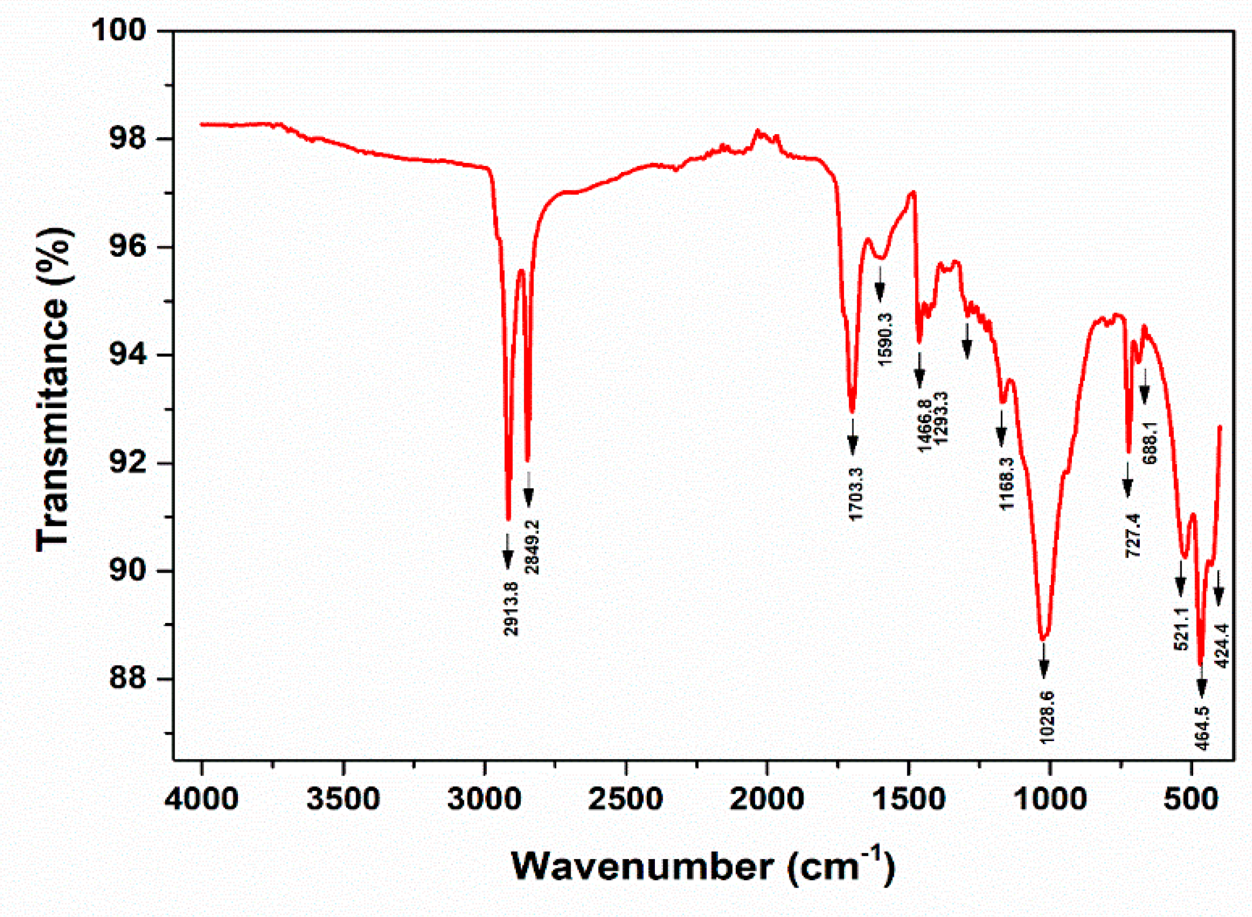
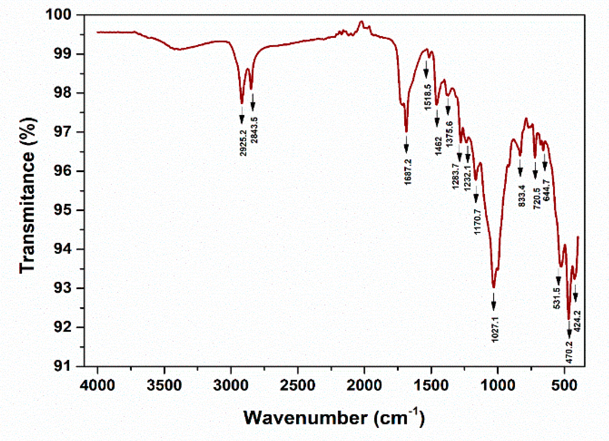
3.4. Fourier Transform Infrared Spectroscopic Analysis (FT-IR)

Fourier Transform Infrared (FT-IR) spectroscopy employs infrared radiation to irradiate polymer particles and subsequently analyzes the wavelengths reflected from these particles to determine their composition. Using the Cary 630 FT-IR Spectrophotometer, the presence of PS in foam spheres sized 3–5 mm (Figure 25) and PE in fragments smaller than 5 mm (Figure 26) was confirmed, which aligns with findings similar to [54].
However, this technique also has limitations: (i) it can identify quantitatively larger samples ≥ 2 mg; and (ii) it is possible to identify the samples that can be mortared for pilling but cannot be applied to foil-type microplastics.
The molecular structure of PS contains CH2 groups and a benzene ring. The saturated C-H bonds show peaks below 3000 cm−1, while the unsaturated C-H bonds originating from the benzene ring result in peaks above 3000 cm−1. According to [62], the peaks around ~3081, ~3059, and ~3025 cm−1 are specific for aromatic C-H stretches, while peaks at 2923 cm−1 and 2850 cm−1 correspond to asymmetric and symmetric CH2 stretches. Peaks at 1600 and 1492 cm−1 are associated with the aromatic ring, 756 cm−1 relates to the out-of-plane C-H bending in the aromatic ring, and 698 cm−1 indicates the bending of the aromatic ring. These same peaks were observed in our study in the case of the PS foam collected from the surface of the water (Figure 25). Peaks at 3060 and 3026 cm−1, along with other peaks at 1600, 1492, and 1452 cm−1 that confirm the presence of benzene rings in the molecule, were also identified in the study of [63] for PS.
In case of the PE fragment, peaks at 2917, 2849, 1469, 1375, and 719 cm−1 were observed (Figure 26) which are specific for the CH2 asymmetric C-H stretch; the CH2 symmetric C-H stretch, the CH3 umbrella mode, and the CH2 rock may be similar with the results of [64].
The ATR-FTIR method, using the Perkin—Elmer Spectrum Two IR spectrometer, was able to detect small particles (<500 µm) of MPs from the filter surface. Two types of MPs, PP and PE, were detected. The measurements in the filtered surface water samples showed the following: UP Floresti—200 µm PP; DW Cluj–Napoca WWTP—200 µm PE; UP Cluj–Napoca WWTP—200 µm and 20 µm PE; DW Cluj–Napoca WWTP—20 µm PE (Figure 27, Figure 28, Figure 29 and Figure 30, Tables S2–S5).
The peaks around ~2955, ~2848, ~1467, and ~720 cm−1 correspond to PE. Meanwhile, PP can be identified by its strong absorption bands at 2845, 2917, and 2979 cm−1.
The infrared spectra of the filter paper are presented in the Supplementary Material (Figure S4 and Table S1). The literature reported that the cellulose ester filters revealed peaks at 900, 1300, and 1400 cm−1. This aspect made it difficult for MPs identification.
The employed spectral techniques Raman and FT-IR enabled the estimation of the qualitative identification of MPs smaller than 500 µm. According to the literature, these methods are complementary [56]. The results showed that both methods confirm the identification of the same type of polymers. The presence of MPs (such as PE, PS, PP, and PC) in various forms and sizes is linked to their uses in food packaging, bottles, toys, textiles, and building materials.

4. Conclusions

It is becoming increasingly apparent that MPs have become a part of our daily lives, and the effects of their presence are starting to manifest. Scientists are engaging in debates regarding new analytical control and monitoring methods. The objective of the paper was to explore the existing methods for the identification and characterization of MPs. The approach included: (i) the occurrence of MPs contamination in the surface water, sediment, and wastewater in the Northwest area of Romania, the Somesul Mic river section from Floresti to Cluj-Napoca WWTP; (ii) isolating and characterization of collected MPs; (iii) and finally the exploration of the possibilities to identify MPs through the use of spectroscopic techniques, namely Raman and FT-IR. By combining these approaches, this research aims to shed light on the extent of MPs contamination and contribute to the development of effective identification and monitoring methods.
The investigations revealed the widespread presence of MPs of various forms, types, and sizes along the course of the Somesul Mic river in the studied area. Both large (1–5 mm) and small (<1 mm) MPs were observed, taking on shapes such as fibers, fragments, foam, foils, and spheres, and exhibiting a range of colors including red, green, blue, purple, pink, white, black, transparent, and opaque. Based on their spectra and the literature data, the identification of PE, PP, and PS was confirmed in all samples. Due to the lack of quantitative determinations, the differences between the sampling points were not possible. Based on the stereomicroscopic investigations, a greater abundance of MPs could be highlighed in in sediments as compared to the water. As we know, microplastics are in continuous mobility in aquatic systems. If responsible waste management measures are not taken, they can migrate from one aquatic system to another until being discharged into the marine ecosystems the most affected one.
Raman techniques using the NRS-7200 Raman Spectrometer and/or the LabRam HR800 system and the ATR FT-IR method using Perkin—Elmer Spectrum Two IR spectrometer were useful for application in MPs identification from environmental samples. The identification of MPs particles smaller than 500 µm to 20 µm could be accomplished using the µRaman or ATR FT-IR method but with some limitations concerning the sample preparation, interferences reduction, availability of polymer spectra database, and human training. Also, the microscopic investigation showed the abundance, particle size (to <1 to >100 µm), and diversification of MPs, demonstrating that it is a method that completes the research of MPs contamination.
Currently, the monitoring of MPs in environmental samples is a time-consuming and costly process. Also there exist some problems related to the standard protocols, experienced researchers and new field and laboratory equipment. The MPs effects on aquatic biota must be seriously studied. The slogan “Our waste on our plate” becomes more and more obvious.

Supplementary Materials

The following supporting information can be downloaded at: https://www.mdpi.com/article/10.3390/w16020233/s1: Figure S1: photos taken during the sampling campaign on Somesul Mic river. Figure S2: images of the river banks taken at the sampling points along the Somesul Mic River. Figure S3: visualization of plastic particles—large, micro, and macro floating MPs separated from Somesul Mic River (surface water and sediment). Figure S4: visualization of plastic particles in the influent of Cluj-Napoca WWTP. Figure S5: SEM images of suspected MPs—decomposing floating MPs. Figure S6: SEM images of suspected MPs without exposure to digestion treatment; scale bar = 500 µm, 50 µm, and 20 µm. Figure S7: ATR-FTIR spectra of the ester cellulose filter membrane. Table S1: assignment of the ATR-FTIR band exhibited by the filter membrane. Table S2: assignment of the ATR-FTIR band exhibited by the UP Cluj-Napoca WWTP 200 µm (PE)—Figure 27. Table S3: assignment of the ATR-FTIR band exhibited by the DW Cluj-Napoca WWTP 200 µm (PE)—Figure 28. Table S4: assignment of the ATR-FTIR band exhibited by the DW Cluj-Napoca WWTP—20 µm (PE)—Figure 29. Table S5: assignment of the ATR-FTIR band exhibited by the UP Floresti 200 µm (PP)—Figure 30 [59,65,66,67,68,69,70,71,72].

Author Contributions

Conceptualization: S.G. and C.S.; data curation: S.G., M.E., A.P. and L.-B.E.; formal analysis: S.G., C.S., A.M.H., E.D.M., A.P., L.-B.E., C.B. and I.A.I.; investigation: A.M.H., M.E., A.P. and L.-B.E.; methodology: S.G., M.E., A.P. and L.-B.E.; project administration: S.G.; resources: S.G.; supervision: S.G. and M.E.; validation: S.G.; visualization: S.G. and C.S.; writing—original draft: S.G. and D.-G.N.; Writing—review and editing, S.G., C.S., M.E., A.P. and L.-B.E. All authors have read and agreed to the published version of the manuscript.

Funding

This work was supported by a grant from the Ministry of Research, Innovation and Digitalization, CNCS-UEFISCDI, project number PN-III-P1-1.1-TE-2021-0073.

Data Availability Statement

Data are contained within the article and Supplementary Materials.

Acknowledgments

The authors express their gratitude to Luculescu Catalin (National Institute for Laser, Plasma and Radiation Physics, Bucharest, Romania); Alexandru Visan (“Coriolan Dragulescu” Institute of Chemistry from Timisoara, Romania); and Ionut Surupacean (Apel Laser), for their support during the stage of MPs identification; and Florinela Pirvu, Florin-Valentin Ciobotaru, Irina Eugenia Lucaciu, Diana Puiu and Mihai Nita-Lazar (National Research and Development Institute for Industrial Ecology—ECOIND Bucharest). Special thanks are extended for providing access to the Raman and FT-IR equipment, supplying necessary materials and offering scientific guidance throughout the research process.

Conflicts of Interest

The authors declare no conflicts of interest.

References

  1. Nava, V.; Frezzotti, M.L.; Leoni, B. Raman Spectroscopy for the Analysis of Microplastics in Aquatic Systems. Appl. Spectrosc. 2021, 75, 1341–1357. [Google Scholar] [CrossRef] [PubMed]
  2. Ferdinand, R. “Plastic”. Encyclopedia Britannica. 22 June 2023. Available online: https://www.britannica.com/science/plastic (accessed on 9 October 2023).
  3. ISO/DIS 24187; Principles for the Analysis of Microplastics Present in the Environment. International Standard Organization: Geneva, Switzerland, 2023.
  4. Geerdes, Z.; Hermann, M.; Ogonowski, M.; Gorokhova, E. A novel method for assessing microplastic effect in suspension through mixing test and reference materials. Sci. Rep. 2009, 9, 10695. [Google Scholar] [CrossRef] [PubMed]
  5. Hurley, R.; Woodward, J.; Rothwell, J.J. Microplastic contamination of river beds significantly reduced by catchment-wide flooding. Nat. Geosci. 2018, 11, 251–257. [Google Scholar] [CrossRef]
  6. Cózar, A.; Echevarría, F.; González-Gordillo, J.I.; Irigoien, X.; Úbeda, B.; Hernández-León, S.; Palma, A.T.; Navarro, S.; García-de-Lomas, J.; Ruiz, A.; et al. Plastic debris in the open ocean. Proc. Natl. Acad. Sci. USA 2014, 111, 10239–10244. [Google Scholar] [CrossRef] [PubMed]
  7. Park, H.; Park, B. Review of Microplastic Distribution, Toxicity, Analysis Methods, and Removal Technologies. Water 2021, 13, 2736. [Google Scholar] [CrossRef]
  8. Jadhav, E.B.; Sankhla, M.S.; Bhat, R.A.; Bhagat, D.S. Microplastics from food packaging: An overview of human consumption, health threats, and alternative solutions. Environ. Nanotechnol. Monit. Manag. 2021, 16, 100608. [Google Scholar] [CrossRef]
  9. Boucher, J.; Friot, D. Primary Microplastics in the Oceans: A Global Evaluation of Sources; IUCN: Gland, Switzerland, 2017; Volume 43. [Google Scholar]
  10. Oluwoye, I.; Machuca, L.L.; Higgins, S.; Suh, S.; Galloway, T.S.; Halley, P.; Tanaka, S.; Iannuzzi, M. Degradation and lifetime prediction of plastics in subsea and offshore infrastructures. Sci. Total Environ. 2023, 904, 904166719. [Google Scholar] [CrossRef]
  11. Available online: https://www.who.int/news/item/03-03-2020-shortage-of-personal-protective-equipment-endangering-health-workers-worldwide (accessed on 10 August 2023).
  12. Available online: https://plasticseurope.org/knowledge-hub/plastics-the-facts-2022/ (accessed on 10 August 2023).
  13. Martinho, S.D.; Fernandes, V.C.; Figueiredo, S.A.; Delerue-Matos, C. Microplastic Pollution Focused on Sources, Distribution, Contaminant Interactions, Analytical Methods, and Wastewater Removal Strategies: A Review. Int. J. Environ. Res. Public Health 2022, 19, 5610. [Google Scholar] [CrossRef]
  14. Schrank, I.; Löder, M.G.J.; Imhof, H.K.; Moses, S.R.; Heß, M.; Schwaiger, J.; Laforsch, C. Riverine microplastic contamination in southwest Germany: A large-scale survey. Front. Earth Sci. 2022, 10, 794250. [Google Scholar] [CrossRef]
  15. Liu, R.-P.; Li, Z.-Z.; Liu, F.; Dong, Y.; Jiao, J.G.; Sun, P.-P.; El-Wardany, R.M. Microplastic pollution in Yellow river, China: Current status and research progress of biotoxicological effects. China Geol. 2021, 4, 585–592. [Google Scholar]
  16. Scherer, C.; Weber, A.; Stock, F.; Vurusic, S.; Egerci, H.; Kochleus, C.; Arendt, N.; Foeldi, C.; Dierkes, G.; Wagner, M.; et al. Comparative assessment of microplastics in water and sediment of a large European river. Sci. Total Environ. 2020, 738, 139866. [Google Scholar] [CrossRef] [PubMed]
  17. Gerolin, C.R.; Nascimento Pupim, F.; Oliveira Sawakuchi, A.; Grohmann, C.H.; Labuto, G.; Semensatto, D. Microplastics in sediments from Amazon rivers, Brazil. Sci. Total Environ. 2020, 749, 141604. [Google Scholar] [CrossRef] [PubMed]
  18. Kiessling, T.; Knickmeier, K.; Kruse, K.; Brennecke, D.; Nauendorf, A.; Thiel, M. Plastic Pirates sample litter at rivers in Germany–Riverside litter and litter sources estimated by schoolchildren. Environ. Pollut. 2019, 245, 545–557. [Google Scholar] [CrossRef] [PubMed]
  19. Huang, S.; Peng, C.; Wang, Z.; Xiong, X.; Bi, Y.; Liu, Y.; Li, D. Spatiotemporal distribution of microplastics in surface water, biofilms, and sediments in the world’s largest drinking water diversion project. Sci. Total Environ. 2021, 789, 148001. [Google Scholar] [CrossRef]
  20. Semmouri, I.; Vercauteren, M.; Van Acker, E.; Pequeur, E.; Asselman, J.; Janssen, C. Presence of microplastics in drinking water from different freshwater sources in Flanders (Belgium), an urbanized region in Europe. Food Contam. 2022, 9, 6. [Google Scholar] [CrossRef]
  21. Ziani, K.; Ioniță-Mîndrican, C.-B.; Mititelu, M.; Neacșu, S.M.; Negrei, C.; Moroșan, E.; Drăgănescu, D.; Preda, O.-T. Microplastics: A Real Global Threat for Environment and Food Safety: A State of the Art Review. Nutrients 2023, 15, 617. [Google Scholar] [CrossRef]
  22. Available online: https://cdn.who.int/media/docs/default-source/wash-documents/microplastics-in-dw-information-sheet190822.pdf (accessed on 13 August 2023).
  23. Mason, S.A.; Welch, V.G.; Neratko, J. Synthetic Polymer Contamination in Bottled Water. Front Chem. 2018, 6, 407. [Google Scholar] [CrossRef]
  24. Chaudhari, S.; Samnani, P. Determination of microplastics in pond water. Mater. Today Proc. 2023, 77, 91–98. [Google Scholar] [CrossRef]
  25. Pojar, I.; Stănică, A.; Stock, F.; Kochleus, C.; Schultz, M.; Bradley, C. Sedimentary microplastic concentrations from the Romanian Danube river to the Black Sea. Sci. Rep. 2021, 11, 2000. [Google Scholar] [CrossRef]
  26. Pojar, I.; Kochleus, C.; Dierke, G.; Ehlers, M.S.; Reifferscheid, G.; Stock, F. Quantitative and qualitative evaluation of plastic particles in surface waters of the Western Black Sea. Environ. Pollut. 2021, 268 Pt A, 115724. [Google Scholar] [CrossRef]
  27. Ding, L.; Mao, R.F.; Guo, X.; Yang, X.; Zhang, Q.; Yang, C. Microplastics in surface waters and sediments of the Wei river, in the northwest of China. Sci. Total Environ. 2019, 667, 427–434. [Google Scholar] [CrossRef] [PubMed]
  28. Organization for Economic Co-operation and Development. Global Plastics Outlook: Policy Scenarios to 2060; OECD Publishing: Paris, France, 2022. [Google Scholar]
  29. Uddin, S.; Fowler, S.W.; Saeed, T.; Naji, A.; Al-Jandal, N. Standardized protocols for microplastics determinations in environmental samples from the Gulf and marginal seas. Mar. Pollut. Bull. 2020, 158, 111374. [Google Scholar] [CrossRef] [PubMed]
  30. Wagner, M.; Scherer, C.; Alvarez-Muñoz, D.; Brennholt, N.; Bourrain, X.; Buchinger, S.; Fries, E.; Grosbois, C.; Klasmeier, J.; Marti, T.; et al. Microplastics in freshwater ecosystems: What we know and what we need to know. Environ. Sci. Eur. 2014, 26, 12. [Google Scholar] [CrossRef] [PubMed]
  31. Asifa, A.; Afroza, A.L.; Md Nazrul, I.; Md Morsaline, B.; Shaikh, T.A.; Md Moshiur, R.; Sheikh, M.R. Microplastics Pollution: A Brief Review of Its Source and Abundance in Different Aquatic Ecosystems. J. Hazard. Mater. Adv. 2023, 9, 100215. [Google Scholar] [CrossRef]
  32. Ashkan, J. Microplastics in the urban atmosphere: Sources, occurrences, distribution, and potential health implications. J. Hazard. Mater. Adv. 2023, 12, 100346. [Google Scholar] [CrossRef]
  33. Enders, K.; Lenz, R.; Stedmon, C.A.; Nielsen, T.G. Abundance, size and polymer composition of marine microplastics >= 10um in the atlantic ocean and their modelled vertical distribution. Mar. Pollut. Bull. 2015, 100, 70–81. [Google Scholar] [CrossRef] [PubMed]
  34. Eriksson, C.; Burton, H. Origins and biological accumulation of small plastic particles in fur seals from macquarie island. Ambio 2003, 32, 380–384. [Google Scholar] [CrossRef]
  35. Cox, K.G.; Covernton, G.A.; Davies, H.J.; Dower, J.F.; Juanes, F.; Dudas, S.E. Human consumption of microplastics. Environ. Sci. Technol. 2019, 53, 7068–7074. [Google Scholar] [CrossRef]
  36. Meyers, N.; Catarino, A.I.; Declercq, A.M.; Brenan, A.; Devriese, L.; Vandegehuchte, M.; De Witte, B.; Janssen, C.; Everaert, G. Microplastic detection and identification by Nile red staining: Towards a semi-automated, cost- and time-effective technique. Sci. Total Environ. 2022, 823, 153441. [Google Scholar] [CrossRef]
  37. Cowger, W.; Gray, A.; Christiansen, S.H.; DeFrond, H.; Deshpande, A.D.; Hemabessiere, L.; Lee, E.; Mill, L.; Munno, K.; Ossmann, B.E.; et al. Critical review of processing and classification techniques for images and spectra in microplastic research. Appl. Spectrosc. 2020, 74, 989–1010. [Google Scholar] [CrossRef]
  38. Bianco, V.; Memmolo, P.; Carcagnì, P.; Merola, F.; Paturzo, M.; Distante, C.; Ferraro, P. Microplastic identification via holographic imaging and machine learning. Adv. Intell. Syst. 2020, 2, 1900153. [Google Scholar] [CrossRef]
  39. Available online: https://www.epa.gov/system/files/documents/2021-09/microplastic-beach-protocol_sept-2021.pdf (accessed on 13 August 2023).
  40. Keck, F.; Vasselon, V.; Tapolczai, K.; Rimet, F.; Bouchez, A. Freshwater biomonitoring in the Information Age. Front. Ecol. Environ. 2017, 15, 266–274. [Google Scholar] [CrossRef]
  41. Marcuello, C. Present and future opportunities in the use of atomic force microscopy to address the physico-chemical properties of aquatic ecosystems at the nanoscale level. Int. Aquat. Res. 2022, 14, 231–240. [Google Scholar]
  42. Pilechi, A.; Abdolmajid, M.; Enda, M. A numerical framework for modeling fate and transport of microplastics in inland and coastal waters. Mar. Pollut. Bull. 2022, 184, 114119. [Google Scholar] [CrossRef] [PubMed]
  43. Sluka, R. Guidelines for Sampling Microplastics on Sandy Beaches. Rocha International Sampling Guide; A Rocha International: London, UK, 2018. [Google Scholar]
  44. Bessa, F.; Frias, J.; Kögel, T.; Lusher, A.; Andrade, J.; Antunes, J.C.; Sobral, P.; Pagter, E.; Nash, R.; O’Connor, I.; et al. Harmonized Protocol for Monitoring Microplastics in Biota; JPI-Oceans BASEMAN Project: Brussels, Belgium, 2019; 30p. [Google Scholar] [CrossRef]
  45. ISO/TR 21960:2020; Plastics—Environmental Aspects—State of Knowledge and Methodologies. International Standard Organization: Geneva, Switzerland, 2020.
  46. Masura, J.; Joel, B.; Gregory, F.; Courtney, A. Laboratory Methods for the Analysis of Microplastics in the Marine Environment: Recommendations for Quantifying Synthetic Particles in Waters and Sediments; NOAA Technical Memorandum NOS-OR&R-48; NOAA Marine Debris Division: Silver Spring, MD, USA, 2015. [Google Scholar]
  47. Schrank, I.; Möller, J.N.; Imhof, H.K.; Hauenstein, O.; Zielke, F.; Agarwal, S.; Löder, M.G.J.; Greiner, A.; Laforsch, C. Microplastic sample purification methods-Assessing detrimental effects of purification procedures on specific plastic types. Sci. Total Environ. 2022, 833, 154824. [Google Scholar] [CrossRef] [PubMed]
  48. Al-Azzawi, M.S.M.; Kefer, S.; Weißer, J.; Reichel, J.; Schwaller, C.; Glas, K.; Knoop, O.; Drewes, J.E. Validation of Sample Preparation Methods for Microplastic Analysis in Wastewater Matrices—Reproducibility and Standardization. Water 2020, 12, 2445. [Google Scholar] [CrossRef]
  49. Kärrman, A.; Schönlau, C.; Engwall, M. Exposure and Effects of Microplastics on Wildlife—A Review of Existing Data; Funded by Swedish Environmental Protection Agency; MTM Research Centre School of Science and Technology Örebro University: Örebro, Sweden, 2016. [Google Scholar]
  50. Wu, X.; Zhao, X.; Chen, R.; Liu, P.; Liang, W.; Wang, J.; Teng, M.; Wang, X.; Gao, S. Wastewater treatment plants act as essential sources of microplastic formation in aquatic environments: A critical review. Water Res. 2022, 221, 118825. [Google Scholar] [CrossRef] [PubMed]
  51. Gerdts, G. (Ed.) Defining the BASElines and Standards for Microplastics ANalyses in European Waters; Project BASEMAN Final report; JPI-Oceans BASEMAN Project, 2019; Volume 25, 25p. [Google Scholar] [CrossRef]
  52. Blair, R.M.; Waldron, S.; Phoenix, V.R.; Gauchotte-Lindsay, C. Microscopy and elemental analysis characterisation of microplastics in sediment of a freshwater urban river in Scotland, UK. Environ. Sci. Pollut. Res. 2019, 26, 12491–12504. [Google Scholar] [CrossRef]
  53. Joshy, A.; Krupesha Sharma, S.R.; Mini, K.G. Microplastic contamination in commercially important bivalves from the southwest coast of India. Environ. Pollut. 2022, 305, 119250. [Google Scholar] [CrossRef]
  54. Mariano, S.; Tacconi, S.; Fidaleo, M.; Rossi, M.; Dini, L. Micro and Nanoplastics Identification: Classic Methods and Innovative Detection Techniques. Front. Toxicol. 2021, 3, 636640. [Google Scholar] [CrossRef]
  55. Schwarzer, M.; Brehm, J.; Vollmer, M.; Jasinski, J.; Xu, C.; Zainuddin, S.; Fröhlich, T.; Schott, M.; Greiner, A.; Scheibel, T.; et al. Shape, size, and polymer dependent effects of microplastics on Daphnia magna. J. Hazard. Mater. 2022, 426, 128136. [Google Scholar] [CrossRef] [PubMed]
  56. Rytelewska, S.; Dąbrowska, A. The Raman Spectroscopy Approach to Different Freshwater Microplastics and Quantitative Characterization of Polyethylene Aged in the Environment. Microplastics 2022, 1, 263–281. [Google Scholar] [CrossRef]
  57. Sharma, S.; Chio, C.; Muenow, D. Raman Spectroscopic Investigation of Ferrous Sulfate Hydrates. In Proceedings of the 37th Annual Lunar and Planetary Science Conference, League City, TX, USA, 3–17 March 2006; Volume 37. [Google Scholar]
  58. Scardaci, V.; Compagnini, G. Raman Spectroscopy Investigation of Graphene Oxide Reduction by Laser Scribing. C 2021, 7, 48. [Google Scholar] [CrossRef]
  59. Primpke, S.; Christiansen, S.H.; Cowger, W.; De Frond, H.; Deshpande, A.; Fischer, M.; Holland, E.B.; Meyns, M.; O’Donnell, B.A.; Ossmann, B.E.; et al. Critical Assessment of Analytical Methods for the Harmonized and Cost Efficient Analysis of Microplastics. Appl. Spectrosc. 2020, 74, 1012–1047. [Google Scholar] [CrossRef] [PubMed]
  60. Leung, M.M.-L.; Ho, Y.-W.; Lee, C.-H.; Wang, Y.; Hu, M.; Kwok, K.W.H.; Chua, S.-L.; Fang, J.K.-H. Improved Raman spectroscopy-based approach to assess microplastics in seafood. Environ. Pollut. 2021, 289, 117648. [Google Scholar] [CrossRef] [PubMed]
  61. Karami, A.; Golieskardi, A.; Choo, C.K.; Romano, N.; Ho, Y.B.; Salamatinia, B. A high-performance protocol for the extraction of microplastics in fish. Sci. Total Environ. 2017, 578, 485–494. [Google Scholar] [CrossRef]
  62. Smith, B.C. The Infrared Spectra of Polymers II: Polyethylene. Spectroscopy 2021, 36, 24–29. [Google Scholar] [CrossRef]
  63. Herman, V.; Takacs, H.; Duclairoir, F.; Renault, O.; Tortai, J.H.; Viala, B. Core double-shell cobalt/graphene/polystyrene magnetic nanocomposites synthesized by in situ sonochemical polymerization. RCS Adv. 2015, 5, 51371–51381. [Google Scholar] [CrossRef]
  64. Smith, B.C. The Infrared Spectra of Polymers III: Hydrocarbon Polymers. Spectroscopy 2021, 36, 22–25. [Google Scholar] [CrossRef]
  65. Käppler, A.; Fischer, D.; Oberbeckmann, S.; Schernewski, G.; Labrenz, M.; Eichhorn, K.-J. Analysis of environmental microplastics by vibrational microspectroscopy: FT-IR, Raman or both? Anal. Bioanal. Chem. 2016, 408, 8377–8391. [Google Scholar] [CrossRef]
  66. Sharma, N.; Sharma, V.; Jain, Y.; Kumari, M.; Gupta, R.; Sharma, S.K.; Sachdev, K. Synthesis and Characterization of Graphene Oxide (GO) and Reduced Graphene Oxide (rGO) for Gas Sensing Application. Macromol. Symp. 2017, 376, 1700006. [Google Scholar] [CrossRef]
  67. Nallasamy, P.; Anbarasan, P.M.; Mohan, S. Vibrational Spectra and Assignments of cis- and Trans-1,4-Polybutadiene. Turk. J. Chem. 2002, 26, 105–111. [Google Scholar]
  68. Gong, Y.; Li, D.; Fu, Q.; Pan, C. Influence of graphene microstructures on electrochemical performance for supercapacitors. Prog. Nat. Sci. Mater. Int. 2015, 25, 379–385. [Google Scholar] [CrossRef]
  69. Syakti, A.D.; Hidayati, N.V.; Jaya, Y.V.; Siregar, S.H.; Yude, R.; Suhendy; Asia, L.; Wong-Wah-Chung, P.; Doumenq, P. Simultaneous grading of microplastic size sampling in the small islands of Bintan Water, Indonesia. Mar. Pollut. Bull. 2018, 137, 593–600. [Google Scholar] [CrossRef]
  70. Chirea, M.; Freitas, A.; Vasile, B.S.; Ghitulica, C.; Pereira, C.M.; Silva, F. Gold nanowire networks: Synthesis, characterization, and catalytic activity. Langmuir 2011, 27, 3906–3913. [Google Scholar] [CrossRef]
  71. Krylova, V.; Dukštienė, N. Synthesis and characterization of AG2S layers formed on polypropylene. J. Chem. 2013, 2013, 987879. [Google Scholar] [CrossRef]
  72. Bhattacharya, S.S.; Chaudhari, S.B. Study on Structural, Mechanical and Functional Properties of Polyester Silica Nanocomposite Fabric. Int. J. Pure Appl. Sci. Technol. 2014, 21, 43–52. [Google Scholar]
Figure 1. Map of sampling points: UP Floresti, DW Floresti, UP Cluj-Napoca WWTP, and DW Cluj-Napoca WWTP (Google maps and QGis—3.26 Buenos Aires Maps Program).
Water 16 00233 g001
Figure 2. Examples of the microscopic visualization of particles suspected to be MPs (indicated by the black arrow) from surface waters concentrated through 20 µm nets in the Floresti area. The picture was taken before the digestion of the organic matter (10×–40× magnifications); scale bar = 1–5 mm.
Water 16 00233 g002
Figure 3. MPs (black arrow) in the form of fibers—(purple, blue, black, and orange) in sediment collected on a 500 µm sieve (possibly polypropylene or polyamide)—UP Floresti; scale bar = 5 mm, 400 µm, 500 µm, 1 mm, 1 mm, and 1 mm.
Water 16 00233 g003
Figure 4. MPs (white arrow) in the form of fibers—(blue, white, and pink) and fragments (pink, white, and blue-green) in sediment collected on a 250 µm sieve—UP Floresti; scale bar = 500 µm, 1 mm, 200 µm, 1 mm, and 1 mm.
Water 16 00233 g004
Figure 5. MPs (white arrow) in the form of fibers (purple) and fragments (transparent) in sediment collected on a 40 µm sieve—UP Floresti; scale bar = 1 mm, 500 µm, 1 mm.
Water 16 00233 g005
Figure 6. MPs (white arrow) in the form of fibers (red and blue), ribbon (transparent and white), foam spheres (white) and fragments (transparent and red) in surface water collected on a 200 µm filter—UP Floresti; scale bar = 5 mm, 2 mm, and 1 mm.
Water 16 00233 g006
Figure 7. MPs (white arrow) in the form of fibers (purple and blue), fragments (brown, yellow, and blue) and foam (white) in sediment collected on the 500 µm sieve—DW Floresti; scale bar = 200 µm, 500 µm, 1 mm, 5 mm, 500 µm, and 500 µm.
Water 16 00233 g007
Figure 8. MPs (white arrow) in the form of fibers (purple and red) and fragments (red) in sediment collected on the 250 µm sieve—DW Floresti; scale bar = 500 µm, 500 µm, 1 mm, and 200 µm.
Water 16 00233 g008
Figure 9. MPs (white arrow) in the form of fibers (purple, blue, pink, and red) and fragments (yellow) in sediment collected on the 40 µm sieve—DW Floresti; scale bar = 1 mm, 500 µm, 1 mm, 500 µm, and 200 µm.
Water 16 00233 g009
Figure 10. MPs (white arrow) in the form of spheres and fragments (blue and red) and fibers (red) in surface water collected using a 20 µm filter—DW Floresti; scale bar = 5 mm, 500 µm.
Water 16 00233 g010
Figure 11. MPs (white arrow) in the form of fibers (brown and green) and fragments (red and white) in sediment collected on the 500 µm sieve—UP Cluj-Napoca WWTP; scale bar = 5 mm, 500 µm, and 5 mm.
Water 16 00233 g011
Figure 12. MPs (white arrow) in the form of purple fibers in sediment collected on the 40 µm sieve—UP Cluj-Napoca WWTP; scale bar = 1 mm and 500 µm.
Water 16 00233 g012
Figure 13. MPs (white arrow) in the form of foam (white) and fibers (purple) in surface water collected on the 20 µm filter—UP Cluj-Napoca WWTP; scale bar = 1 mm.
Water 16 00233 g013
Figure 14. MPs (white arrow) in the form of fibers (purple, blue, and pink) and fragments (blue and pink) in sediment collected on the 40 µm sieve—DW Cluj-Napoca WWTP; scale bar = 200 µm, 500 µm, 1 mm, 1 mm, and 500 µm.
Water 16 00233 g014
Figure 15. MPs (white arrow) in the form of fibers (purple, pink, and transparent) and fragments (transparent and yellow) in sediment collected on the 250 µm sieve—DW Cluj-Napoca WWTP; scale bar = 1 mm, 500 µm, 200 µm, 1 mm, 200 µm, and 500 µm.
Water 16 00233 g015
Figure 16. MPs (white arrow) in the form of fibers (blue) and fragments (red) in sediment collected on the 500 µm sieve—DW Cluj-Napoca WWTP; scale bar = 500 µm and 200 µm.
Water 16 00233 g016
Figure 17. MPs (white arrow) in the form of fibers (purple, blue, and pink) and fragments (transparent and orange) in surface water collected on the 20 µm filter—DW Cluj-Napoca WWTP; scale bar = 1 mm, 1 mm, 2 mm, and 500 µm.
Water 16 00233 g017
Figure 18. MPs (white arrow) in the form of fibers (purple and blue) and fragments (green and red) isolated from the WWTP effluent without concentration of the sample; scale bar = 2 mm, 1 mm, 500 µm, 500 µm, and 200 µm.
Water 16 00233 g018
Figure 19. SEM images of suspected MPs: (a) sphere and fragments in particles size of 475 nm to 66 µm, scale bar = 10 µm; and (b) fibers in particles sizes of 23.49 to 407 µm, scale bar = 100 µm.
Water 16 00233 g019
Figure 20. Raman spectra of the standard MPs: (a) PE 40–48 µm and 3 mm; (b) PS 3 mm; (c) PP 3 mm.
Water 16 00233 g020aWater 16 00233 g020b
Figure 21. Raman spectra: (a) sediment UP Floresti—PP (white fragment) 4 mm, spectra compared to reference spectra PP (shown in dark orange); (b) sediment UP Floresti—PP (green fragment) 5 mm, spectra compared to reference spectra PP (shown in orange); (c) wastewater influent—PE (white fragment) 2 mm, spectra compared to reference spectra PE (shown in orange); (d) sediment UP WWTP—fragment 500 µm—the identification was unclear, spectra compared to reference spectra PE (shown in light blue); (e) sediment UP Cluj-Napoca WWTP—fragments—PE, 1 mm, 4 mm, spectra compared to reference spectra PP (shown in orange).The ellipses reveled the MPs peaks similarity with the standard spectra.
Water 16 00233 g021aWater 16 00233 g021b
Figure 22. Raman spectra—sediment UP Cluj-Napoca WWTP. Fragments 3 mm and brown sphere 2 mm—suspected to be PE.
Water 16 00233 g022
Figure 23. Raman spectra recorded at the highlighted locations—sediment samples, identifications on filter paper: (a) PP identification (UP Floresti): exposure time 30 s, accumulation 10, center wavenumber 740.11 cm−1, Z position 16061.1 µm, binning interval 240–374, valid channel 1–2048, laser wavelength 784.74 nm, resolution 9.02 cm−1, 0.61 cm−1/pixel, objective lens LMPLFLN 10×, slit 200 × 1000 µm, aperture d-4000 µm, laser power 56.6 mW, CCD temperature −70 °C; (b) PS identification (DW Cluj Napoca WWTP): exposure time 30 s, accumulation 20, center wavenumber 1520.21 cm−1, Z position 17,003.6 µm, binning interval 240–374, valid channel 1–2048, laser wavelength 531.94 nm, resolution 4.79 cm−1, 1.30 cm−1/pixel, objective lens LMPLFLN 10×, slit 50 × 1000 µm, aperture d-4000 µm, laser power 5.5 mW, CCD temperature −70 °C; (c) PC identification (DW Cluj Napoca WWTP): exposure time 30 s, accumulation 10, center wavenumber 740.11 cm−1, Z position 17,053.7 µm, binning interval 240–374, valid channel 1–2048, laser wavelength 784.74 nm, resolution 9.02 cm−1, 0.61 cm−1/pixel, objective lens LMPLFLN 10×, slit 200 × 1000 µm, aperture d-4000 µm, laser power 56.4 mW, CCD temperature −70 °C; (d) PE or PP unclear identification—green fragment (influent of Cluj Napoca WWTP): exposure time 20 s, accumulation 10, center wavenumber 1520.21 cm−1, Z position 17,213.7 µm, binning interval 240–374, valid channel 1–2048, laser wavelength 531.94 nm, resolution 4.79 cm−1, 1.30 cm−1/pixel, objective lens LMPLFLN 10×, slit 50 × 1000 µm, aperture d-4000 µm, laser power 5.6 mW, CCD temperature −70 °C.
Water 16 00233 g023aWater 16 00233 g023b
Figure 24. µRaman spectra recorded at the highlighted locations—surface water samples: (a) filter membrane spectra; (b) UP Cluj-Napoca WWTP 20 µm—potentially PP among others [57]; (c) UP Cluj-Napoca WWTP 20 µm— a C compound among others [58]; (d) UP Cluj-Napoca WWTP 20 µm—potentially TiO2 (anatase phase), white pigment [57]; (e) UP Cluj-Napoca WWTP 20 µm- potentially α-Fe2O3 or FeO(OH)nH2O, red pigment; (f,g) UP Cluj-Napoca WWTP 200 µm—no clear Raman bands, only fluorescence; (h) DW Cluj-Napoca WWTP 20 µm—potentially PP among others [57]; (i) DW Cluj-Napoca WWTP 20 µm—potentially PP among others [54]; (j,k) DW Cluj-Napoca WWTP 20 µm—a C compound among others [58]; (l,m) DW Cluj-Napoca WWTP 200 µm—clear evidence of PE [54]; (n) UP Floresti 200 µm—no clear Raman bands; (o) UP Floresti 200 µm—a C compound [58].
Water 16 00233 g024aWater 16 00233 g024bWater 16 00233 g024c
Figure 25. Infrared spectra of PS foam measuring 3–5 mm (floating MPs).
Water 16 00233 g025
Figure 26. Infrared spectra of PE fragment <5 mm (floating MPs).
Water 16 00233 g026
Figure 27. ATR-FTIR spectra—PE, UP Cluj—Napoca WWTP 200 µm (water sample).
Water 16 00233 g027
Figure 28. ATR-FTIR spectra—PE, DW Cluj—Napoca WWTP 200 µm (water sample).
Water 16 00233 g028
Figure 29. ATR-FTIR spectra—PE, DW Cluj—Napoca WWTP 20 µm (water sample).
Water 16 00233 g029
Figure 30. ATR-FTIR spectra—PP, UP Floresti 200 µm (water sample).
Water 16 00233 g030
Table 1. Field data—visual characterization of floating plastics and other wastes.
Sampling PointTypeDimensionColorNo. Total of ParticlesClassification
UP Floresti
left bank: low water level, clear water, waste island on the right bank, flow speed approx. = 0.58 m/s
Fragment>30 mmblack, green, blue5Macro
Fragment—foil≥20 mmwhite, green/blue2Macro
Sphere<5 mmred, brown2Large
Fragment~10 mmwhite-gray1Meso
Foam~5 mmyellow1Large
Polystyrene pieces>10, 20, 30 mmwhite3Meso/Macro
Non–plastics and other wastes
Surgical mask fragment/cellulose>30 mmgreen1-
Fragments of aluminum packaging>50 mmblue1-
Electronic parts20 mmwhite 1-
Aluminum plugs~20 mmgray2-
Textile>30 mm 1-
Plastic coated wire~2, 10, 12 cmgray, white, blue3-
Construction
materials (brick,
cement, etc.)
--abundantly-
DW Floresti
left bank: under construction, cloudy water,
flow rate approx. = 0.40 m/s
Fragment-foil10 mmtransparent1Meso
Fragment30 mmtransparent1Meso
Sphere<5 mmgreen1Large
Polystyrene foam5 mmwhite5Large
Foam/sponge>30 mmyellow1Macro
Fragment>30 mmblue1Macro
Plastic toy piece>30 mmred1Macro
Non–plastics and other wastes
Construction
materials
--abundantly-
UP Cluj-Napoca WWTP
left bank:
low level,
flow rate approx. = 0.64 m/s
Polystyrene spheres, foam<5 mmwhiteabundantlyLarge
Pieces of polystyrene>20 mmwhiteabundantlyMeso
Fragment<5 mmwhite1Large
Fragment~3, 5, 10 mmwhite3Large/Meso
Non–plastics and other wastes
Cigarette butts>10 mmbrown1Meso
Plastic waste from toys and packaging>10 cm
>30 cm
2Macro
Pet bottles--1-
DW Cluj –Napoca WWTP
left bank: waste on the bank, bags and foils under sediment and stones
flow rate approx. = 0.62 m/s
Fragment>30 mmtransparent1Macro
Fragment~20 mmblack1Meso
Polystyrene foam spheres~5 mmwhite1Large
Pieces of polystyrene~5 mmwhite>10Large
Non–plastics and other wastes
Textile>30 mm---
Construction material--abundantly-
Note: Macro: macroplastics; Large: large microplastics; Meso: Mesoplastic; Micro: microplastic.; abundantly: the materials could not be counted.
Disclaimer/Publisher’s Note: The statements, opinions and data contained in all publications are solely those of the individual author(s) and contributor(s) and not of MDPI and/or the editor(s). MDPI and/or the editor(s) disclaim responsibility for any injury to people or property resulting from any ideas, methods, instructions or products referred to in the content.

