Abstract
Accurate and reliable wave forecasting is crucial for optimizing the performance of various marine operations, such as offshore energy production, shipping, and fishing. Meanwhile, predicting wave height and wave energy is crucial for achieving sustainability as a renewable energy source, as it enables the harnessing of the power of wave energy efficiently based on the water-energy nexus. Advanced wave forecasting models, such as machine learning models and the semi-analytical approach, have been developed to provide more accurate predictions of ocean waves. In this study, the Sverdrup Munk Bretschneider (SMB) semi-analytical approach, Emotional Artificial Neural Network (EANN) approach, and Wavelet Artificial Neural Network (WANN) approach will be used to estimate ocean wave parameters in the Gulf of Mexico and Aleutian Basin. The accuracy and reliability of these approaches will be evaluated, and the spatial and temporal variability of the wave field will be investigated. The available wave characteristics are used to generate hourly, 12-hourly, and daily datasets. The WANN and SMB model shows good performance in the daily prediction of the significant wave height in both case studies. In the SMB model, specifically on a daily time scale, the Nash–Sutcliffe Efficiency (NSE) and the peak deviation coefficient (DCpeak) were determined to be 0.62 and 0.54 for the Aleutian buoy and 0.64 and 0.55 for the Gulf of Mexico buoy, respectively, for significant wave height. In the context of the WANN model and in the testing phase at the daily time scale, the NSE and DCpeak indices exhibit values of 0.85 and 0.61 for the Aleutian buoy and 0.72 and 0.61 for the Gulf of Mexico buoy, respectively, while the EANN model is a strong tool in hourly wave height prediction (Aleutian buoy (NSEEANN = 0.60 and DCpeakEANN = 0.88), Gulf of Mexico buoy (NSEEANN = 0.80 and DCpeakEANN = 0.82)). In addition, the findings pertaining to the energy spectrum density demonstrate that the EANN model exhibits superior performance in comparison to the WANN and SMB models, particularly with regard to accurately estimating the peak of the spectrum (Aleutian buoy (DCpeakEANN = 0.41), Gulf of Mexico buoy (DCpeakEANN = 0.59)).
1. Introduction
Ocean wave forecasting is a critical aspect of ocean engineering and management, as it plays an essential role in the design, construction, and operation of offshore structures and coastal protection systems [1,2]. Accurate and reliable wave forecasting is crucial for optimizing the performance of various marine operations, such as shipping, offshore energy production, and fishing [3,4]. Traditional wave forecasting models rely on physical and statistical models, which have certain limitations in predicting complex wave phenomena accurately [5,6,7,8]. Therefore, there is a need to develop advanced wave forecasting models that can provide more accurate and reliable predictions of ocean waves.
The ocean is a dynamic and complex system that is constantly changing due to various environmental factors, such as wind, temperature, and currents [9]. The behavior of ocean waves is of significant interest to the ocean engineering community, as it has a significant impact on the design and operation of various marine structures [10]. Accurate and reliable wave forecasting is essential for optimizing the performance of these structures and ensuring the safety of personnel working in the marine environment [11].
In recent years, there has been significant research and development in the field of wave forecasting, with various models and methods proposed to predict the behavior of ocean waves [12,13,14]. Over the years, various wave forecasting models have been developed using different approaches, such as physical, statistical, and machine learning models [15,16,17,18,19,20,21].
Statistical models, on the other hand, are based on empirical relationships between wave parameters and environmental conditions, such as wind speed, atmospheric pressure, and sea surface temperature [22]. These models are relatively simple and require less computational effort than physical models, but they are limited in their ability to capture the nonlinear relationships between the input and output parameters [23].
However, numerical models have been developed to predict wave characteristics under different environmental conditions [24,25]. For instance, Boussinesq models have been used extensively to predict wave conditions in coastal and offshore zones [26]. Using a fully nonlinear Boussinesq model, Gao et al. [27] simulated wave motion and interaction in the harbor. Consideration was given to two types of harbor oscillations: the harbor resonance directly induced by the regular long waves and the nonlinear harbor resonance induced by the bichromatic short wave groups. In another study, Gao et al. [28] numerically simulated the low-frequency waves inside a long port near the reef, which is excited by short wave groups. They evaluated the effects of the reef ridge slope on the characteristics of low-frequency waves.
In the past decade, several complex numerical models have been developed for wave forecasting [29]. Meanwhile, the implementation of large numerical models requires a substantial quantity of depth, meteorological, and oceanographic data [30]. In some regions, these data are unavailable, making numerical modeling difficult and expensive. Moreover, based on the initial estimates, the use of these models is often not economically justified. Therefore, engineers tend to utilize simple prediction methods based on internal relationships in these situations [31]. These techniques are sufficiently precise for initial estimations and simple situations with minimal local effects.
In recent years, the semi-analytical approach has been applied, besides other methods such as machine learning algorithms and numerical models, to improve wave estimation accuracy and to study the spatial and temporal variability of ocean waves [19,32]. This approach combines the linear theory of ocean waves with empirical data on wave spectra to estimate wave characteristics in deep water conditions. Researchers have used this approach to estimate wave parameters from satellite data, buoy measurements, and radar observations [33].
The Sverdrup Munk Bretschneider (SMB) semi-analytical approach is a widely used method for estimating ocean wave parameters. It was first introduced in the late 1940s and has since been refined and adapted by numerous researchers in the field of oceanography [34]. The SMB approach has been used for wave estimation in various oceanographic applications, including weather forecasting, ocean engineering, and coastal management. Others have incorporated the SMB approach into numerical models to simulate wave propagation and wave–structure interactions [35,36]. Soomere et al. [37] highlighted that semi-analytical techniques, such as the SMB method, continue to demonstrate efficacy in the preliminary estimation of oceanic wave behavior. However, as third-generation models and numerical approaches continue to advance, these methods are increasingly being considered as supplementary options to the SMB method. Nevertheless, the utilization of numerical models in wave simulation is hindered by their significant computational expense and the inherent difficulty in obtaining appropriate input data. In order to attain the desired outcomes within the SMB model, it is imperative to employ the concept of effective fetch. Nevertheless, small- and medium-sized businesses (SMBs) do not achieve optimal performance when it comes to limited fetching [38]. Studies have demonstrated that due to the nonlinear nature of the wave–wind process, old fashion SMB model may not be able to simulate it accurately [39,40]. The consideration of this issue is imperative in order to ensure accurate and dependable production in nearshore to coastal areas [41,42]. Nevertheless, there is a lack of empirical research comparing the efficacy of this approach in deep water scenarios with contemporary machine learning techniques.
In addition, machine learning models have emerged as a promising approach for wave forecasting, as they can capture the nonlinear relationships between the input and output parameters and can learn from the historical data to improve the accuracy of the predictions [43,44,45]. Fan et al. [46] employed the LTSM long-term–short-term memory network to forecast the wave height in various water stations within the Gulf of Mexico for the subsequent 1 and 6 h time scales. The findings of this study indicate that the long-short-term memory (LSTM) model has demonstrated its ability to forecast the outcomes of stable conditions. Dai et al. [47] have made predictions regarding the wave height in the Gulf of Mexico by employing the Conditional Restricted Boltzmann Machine–Deep Network (CRBM-DBN) methodology. The findings of this study demonstrate that, in the context of short-term wave height forecasting, the error indicator for future predictions within a 12 h time frame is a significant factor. Within the span of 26 degrees north latitude, this quantity exhibits a gradual decline as the geographical latitude increases toward the north and decreases toward the south. Londhe et al. [48] made predictions regarding the future trajectory of India. The prediction for the upcoming 24 h period has been generated utilizing a numerical model, followed by the application of a neural network to rectify any inaccuracies. The findings of this study demonstrate that the utilization of this approach yields a discernible enhancement in the accuracy of predictions. In a study conducted by James et al. [49], various machine learning techniques were employed to forecast wave height and period in the Monterey Bay region. In the aforementioned study, two distinct methodologies were employed for the purpose of wave prediction. The analysis of wave height involves the utilization of a multi-layer neural network comprising three hidden layers. The support vector machine has also utilized the categorization of wave repetition period. The outcomes indicate a strong concordance between the predicted target values and the machine learning, thereby demonstrating a high confidence coefficient of the model.
Among the machine learning models, artificial neural networks (ANNs) have been widely used for wave forecasting due to their ability to learn from the data and their ability to model the nonlinear relationships between the input and output parameters [50,51,52]. However, ANNs have certain limitations, such as the risk of overfitting and the difficulty in interpreting the results [53]. To address these limitations, several advanced neural network models, such as Emotional Artificial Neural Networks (EANNs) and Wavelet Artificial Neural Networks (WANNs), have been proposed. The neuro-wavelet technique was employed to forecast wave height in buoys numbered 42040, 42039, 41004, and 41041 located in the Gulf of Mexico during the fifth event of the Great Hurricane Katrina in 2005. Dean (2007), Gustav (2008), Ike (2008), and Ayran (2011) are the events under consideration [54]. The neural network model utilized wavelet decomposition as its input, wherein the wave height time series was decomposed into three, five, and seven levels. The researchers demonstrated that the wavelet neural network technique can be effectively resolved. The issue pertaining to the precise forecasting of severe storm occurrences was addressed. The application of the EANN model has been extended in the field of rainfall and runoff prediction research [55,56,57]. However, its potential for predicting sea waves has not yet been explored. Furthermore, a comprehensive evaluation of this novel approach in relation to existing models that have been extensively studied in the domain of wave characteristic prediction has not been conducted.
Wave forecasting has overlooked conducting a direct comparison between nearly conventional semi-analytical methods and emerging hybrid machine learning models. The significance of the present investigation pertains to the comparative and evaluative analysis of various methodologies employed for the estimation of oceanic wave characteristics. In this study, we will use the SMB semi-analytical, EANN, and WANN approaches to estimate ocean wave parameters in the Gulf of Mexico and the Aleutian Basin. The chosen regions were designated in order to assess the performance of the models independently from the local environmental conditions. We will evaluate the accuracy and reliability of these approaches in comparison to each other and investigate the spatial and temporal variability of the wave field. These models are used to model the nonlinear relationships between the input parameters and the output wave parameters, which are difficult to capture using traditional physical models. Furthermore, it is important to note that buoys and models utilized for the purpose of recording sea waves possess distinct capabilities in relation to the time scale at which marine data is recorded. Therefore, possessing knowledge and understanding of models that are compatible with these specific time scales can facilitate the selection of an appropriate model for wave prediction. Thus, in this study, the efficiency of the mentioned models in different time scales was evaluated using hourly data, 12 h averages, and daily averages. The findings of this study can be applied to improve the accuracy of wave forecasting models and to aid in the design of safe and efficient marine structures in these regions.
2. Study Area and Dataset
The study area for this research encompasses two distinct regions: the Aleutian Basin and the Gulf of Mexico.
The Aleutian Basin is a deep-water basin located in the northern Pacific Ocean, extending from the Aleutian Islands to the Kamchatka Peninsula. The study area for this research encompasses a region within the Aleutian Basin, between 50° N to 55° N latitude and 170° E to 180° longitude (Figure 1a). The Aleutian Basin is a complex oceanic region characterized by diverse oceanographic conditions. It is influenced by several oceanic currents, including the Alaska Coastal Current and the Aleutian Current. The region is subject to strong winds and storms, which contribute to a highly variable wave climate in the Aleutian Basin, with significant variations in wave height, period, and direction. The Aleutian Basin is an important region for several marine activities, including fishing, shipping, and oil and gas production. Accurate estimation of ocean wave parameters is necessary for the design and operation of these marine structures. Therefore, understanding the spatial and temporal variability of the wave field in the Aleutian Basin is crucial for these activities [58,59,60,61].
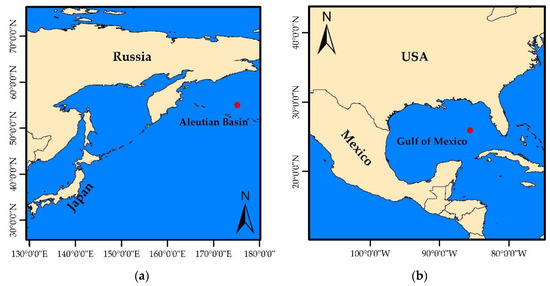
Figure 1.
The location of study area and buoy situation based on NOAA National Data Buoy Center (NDBC). (a) Buoy 46070, at 55°0′30″ N 175°10′59″ E, at a depth of 3865 m (Aleutian Basin), and (b) Buoy 42003, at 25°55′31″ N 85°36′58″ W, at 3273 m (Gulf of Mexico).
The Gulf of Mexico is a large body of water located in the Atlantic Ocean, bordered by the United States to the north, Mexico to the west and south, and Cuba to the southeast. The study area for the Gulf of Mexico is located between 15° N to 30° N latitude and 85° W to 100° W longitude (Figure 1b). The Gulf of Mexico is an important region for several marine activities, including shipping, oil and gas production, and commercial fishing. Accurate estimation of ocean wave parameters is necessary for the design and operation of these marine structures. The Gulf of Mexico is also vulnerable to extreme weather events, including hurricanes, which can cause significant damage to coastal communities and marine structures [62,63,64].
The regions that were selected were specified in order to evaluate the performance of the models in a manner that is independent of the environmental factors that are present in the local area.
NOAA National Data Buoy Center (NDBC) collected the wind–wave data used in this investigation (https://www.ndbc.noaa.gov/ accessed on 12 February 2022). Figure 1 displays the locations of NDBC stations in the Aleutian Basin and the Gulf of Mexico. Depending on the timeline, buoys and models used to record sea waves have varying capacities. Knowing which models are consistent with certain time scales might thus aid in the selection of a wave prediction model. Therefore, the available wave characteristics are used to generate datasets, including hourly, 12-hourly, and daily averages. Table 1 presents the statistics of the used wave characteristics data for the study regions. For the current study, 80% percent of the available data is used for training, while the remaining 20% is retained for testing.

Table 1.
The statistics of the observed time series for Aleutian Basin and Gulf of Mexico.
3. Materials and Methods
In this section, we will introduce the SMB semi-analytical approach, the EANN, and the WANN method.
3.1. Sverdrup Munk Bretschneider
The SMB semi-analytical approach is a commonly used method for analyzing ocean dynamics, particularly in the study of waves and currents. The SMB approach uses mathematical equations to model the interactions between the ocean and the atmosphere, as well as the effects of tides and waves. This method has been widely used in oceanographic research and is still an important tool for understanding ocean dynamics.
SMB equations are based on dimensionless analysis. These equations are presented for deep water [19]. If the wind with speed u is over a fetch length of F, a wave is produced with a significant wave height Hs and a significant wavelength Ts in a region with depth d of the equations, and the following are obtained:
The aforementioned values for Hs and Ts only occur when the wind blows for t minute on an F fetch length, as determined by the expression below.
If min t < tmin, then we calculate F for a certain t from Equation (3) and then add the new F to Equations (1) and (2). In this case, the sea has a limited wind duration, and the wavelength is controlled by the wind duration. If t > tmin, the height and length of the waves are controlled by the specific wavelength. The equations for the deep-water region are summarized as follows:
3.2. Emotional Artificial Neural Network
In recent years, the use of machine learning methods has become increasingly popular in various fields of research, including oceanography. EANNs are types of neural networks that are designed to evolve and adapt to changing conditions, making them well suited for modeling complex systems like the ocean.
The Emotional Artificial Neural Network (EANN) is a further development of the Artificial Neural Network (ANN) [65,66]. It allows neurons to create agents that can alter cognitive, emotional, and production functions as required. In other words, EANN models are an updated generation of conventional ANN models that incorporate an artificial sensing unit that can release hormones to regulate the operation of nodes (neurons) and hormone weights that can be adjusted based on the input and output values of the nodes [67,68]. As shown in Figure 2, each node of the EANN can repeatedly receive and transmit data between the input and output components, resulting in the production of dynamic hormones Ha, Hb, and Hc. First, the coefficients change depending on the relationship between the input and output, and then, after multiple iterations, they are enhanced during the model training phase. Hormonal coefficients influence the node characteristics, including the activation function, net performance, and mass. In Figure 2, the solid and dashed lines represent the neuronal and hormonal information pathways, respectively. The first output of the EANN model comprised Ha, Hb, and Hc hormone secretors with ith nerve cell output (Equation (7)).
where , and represent the output, hidden, and input neurons, respectively. f is the neuron function activator, , and are the function weight activation values, and , and show the neuron weights [57]. Using Equation (8), the model hormone values were evaluated and enforced on the neuron network.
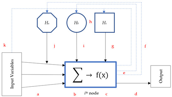
Figure 2.
The unit of EANN model (a to k are the process steps).
In the training phase of the EANN model, the glandity index should be calibrated in order to assign the proper quantity of hormones to the glands [65].
In this study, the network is trained using the Levenberg–Marquardt algorithm. It is a modified version of Newton’s classical algorithm, which is used to find the optimal solution for minimization-based problems. This method, like Newton’s method, considers an approximation for the Hessian matrix in changing weights (Equation (9)).
where x represents the weights of the neural network, J represents the Jacobian matrix of the network execution criterion to be minimized, and e represents the residual error vector. When it is zero, the preceding equation is identical to Newton’s method, which employs Hessian’s method; however, when it is a large value, it becomes a gradient reduction relationship with a short time interval. The results of Newton’s method will be extremely close to the minimum error rate. This algorithm is highly effective and stable [69,70]. Levenberg–Marquardt is designed to minimize sum-of-square error functions. To ensure linear approximation validity, the Levenberg–Marquardt algorithm minimizes the error function and reduces the step size. This iterative algorithm finds a local minimum of a multivariate function that is the sum of squares of several non-linear, real-valued functions. It is a standard method for non-linear least-square problems, used in many fields for data-fitting applications.
3.3. Wavelet Artificial Neural Network
The wavelet transform is a powerful tool for analyzing non-stationary signals, which are signals that vary in time and frequency. In the field of ocean engineering, the wavelet transform has been used extensively for the analysis of ocean waves [15].
The wavelet transform is based on the decomposition of a signal into a series of wavelets, which are small waves that are localized in both time and frequency. The decomposition is performed by convolving the signal with a series of wavelet functions, which are scaled and translated versions of a mother wavelet. The resulting wavelet coefficients represent the contribution of each wavelet to the original signal [65,71,72].
One of the main advantages of the wavelet transform is its ability to capture localized features in a signal. This makes it particularly useful for analyzing ocean waves, which can exhibit a wide range of behaviors over different time and frequency scales. By decomposing the wave signal into a series of wavelets, the wavelet transform can identify and quantify specific features of the wave, such as its period, amplitude, and phase.
The discrete wavelet transform (DWT) is widely employed as the predominant wavelet transform method. Nevertheless, the critically sampled DWT exhibits a reduced sampling density in the time–frequency plane and also lacks the desirable property of shift invariance. This phenomenon has a significant impact on the performance of signal decomposition and compression techniques. The proposal of the redundant (or expansive) wavelet transform aimed to enhance the efficacy of signal decomposition and compression. The dyadic wavelet transform is an example of a redundant wavelet transform. According to Qin et al. [73], the shift-invariant property of this method allows it to exhibit exceptional efficacy in a wide range of signal-processing applications. Therefore, in this study, CWT was used to decompose the wave characteristic.
The following equation describes how to define the time-scale wavelet transform of a continuous-time series:
Equation (11) is a relation with two variables, and , in which is the scale parameter (inverse of frequency) and is the transfer parameter. The symbol * is the complex that is used for conjugate. , the mother wavelet, and , the transferred and scaled versions (daughter wavelets), are obtained from this function. That is, the mother wavelet is a template for other windows. The symbol indicates the multiplication of two functions in the signal space [74].
The combination of wavelet theory and neural network concepts results in the creation of a wavelet neural network, whose application can serve as an alternative to conventional neural networks for estimating and approximating nonlinear functions with optional coefficients. In feedforward neural networks, the hidden layer activation function is sigmoid, whereas, in wavelet neural networks, wavelet functions are regarded as the activation function of the feedforward network’s hidden layer. Figure 3 displays the WANN model’s schematic diagram. In addition, the scale change of the wavelets and their weights are optimized. The training and validation of the wavelet neural network entails the following significant steps [75,76].
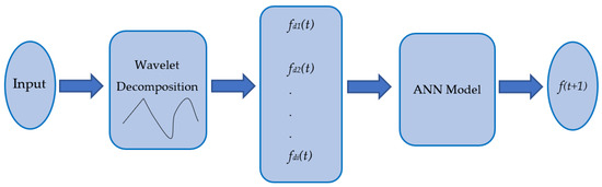
Figure 3.
Structure of the proposed WANN model.
- The input data are used for training and validating the network;
- b—Under the specified conditions, the mother wavelet is transformed into the daughter wavelet by applying the transfer coefficients and the appropriate scale;
- Types of child wavelets replace the activation functions of the neurons in the hidden layer of the neural network;
- The created violet neural network is trained with the training-related dataset.
- The overall performance of the wavelet network is analyzed by examining the method for estimating the precision of measurement data, and with the part of the network’s approval, the training phase is concluded. Otherwise, the steps leading up to the optimal state are evaluated. It has been demonstrated as an example of a three-layer network structure with an input layer, a hidden layer, and an output layer. Meanwhile, the Levenberg–Marquardt algorithm was applied to train the model.
3.4. Wave Energy Density Spectrum
The random behavior of the vertical fluctuations of the water level relative to the average sea level (η = 0) at a specific point is represented by its autocorrelation function (Equation (12)), while the variation of the variable η is constant.
The Wiener–Khintchine theorem holds significant relevance in the analysis of waves associated with maritime accidents. This theory establishes the connection between the autocorrelation function in the temporal domain and the energy spectrum () in the frequency domain. Based on the theoretical framework under consideration, assuming the stationary nature of sea fluctuations, the wave spectral density can be mathematically represented as the Fourier transform of the autocorrelation function (Equation (13)).
The utilization of the fast Fourier transform (FFT) method was employed in order to extract the spectrum, as the processing is conducted on a discrete time series.
3.5. Efficiency Criteria
To evaluate the accuracy of the models and compare the results of the estimated models to the measured values of the wave height, tests proposed by Jacovides [77] were carried out in this study. In addition to these two indices, it is recommended to use the t index and Nash–Sutcliffe efficiency (NSE) and DCpeak to evaluate the model peak capture performance.
where Pi is the predicted value of the wave, Oi is the observed value, N is the number of observations, RMSE is the root mean square error, and SD is the standard deviation in these equations. Equation (14) can be used to compare the model’s efficiency in capturing the time series’ peak values, where Pipeak is the predicted peak value of the wave parameter, Oipeak is the peak observed value, and Np is the number of peak observations. The dispersion parameters SI, bias, and t, as well as the correlation coefficient, were used to evaluate the SMB, EANN, and WANN models.
4. Results and Discussion
This section evaluates and compares the effectiveness of the semi-analytical model, EANN model, and WANN model in predicting the properties of wind-generated waves in deep water.
4.1. Sverdrup Munk Bretschneider
Figure 4 and Figure 5 show the results for Buoy 46070 (Aleutian Basin) and Buoy 42003 (Gulf of Mexico), respectively. Hourly data, 12 h average data, and daily average data are the three modes in which the results are presented. According to the results displayed in Figure 4 for the Aleutian Basin (Buoy 46070), the semi-analytical SMB method performs better in daily average data than hourly data and 12 h average data.
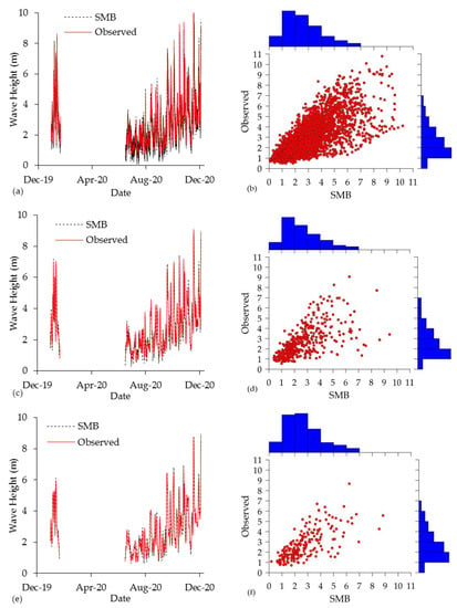
Figure 4.
A comparison of the wave height data for Buoy 46070 in Aleutian Basin with the prediction results of SMB model, (a,b) hourly wave data, (c,d) 12 h average wave data, and (e,f) daily wave data.
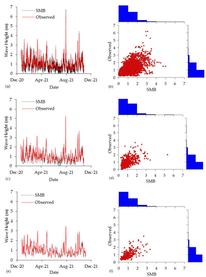
Figure 5.
A comparison of the wave height data for Buoy 42003 in Gulf of Mexico with the prediction results of SMB model, (a,b) hourly wave data, (c,d) 12 h average wave data, and (e,f) daily wave data.
The comparison of wave period and wave propagation direction for Buoy 46070 is presented in Appendix A and Figure A1. Figure A2 displays the same outcomes pertaining to Buoy 42003.
Similar to the outcomes of the semi-analytical model’s prognostication for Buoy 46070, the efficacy of this model is superior in forecasting wave height for daily average data (Figure 5). The model’s performance outcomes and statistical evaluations, which are displayed in Table 2, endorse this fact. It must be noted that the limited fetch length cases, limited duration of oscillation cases, and overall case are at a significance level of 0.01. The improved performance of the daily time scale result in this model can be attributed to the smaller dataset size and lower peak values (Aleutian Basin wave height DCpeakDaily = 0.54 and Gulf of Mexico wave height DCpeakDaily = 0.55). Nevertheless, as the frequency of fluctuations in the hourly data rises, the efficacy of the model diminishes. However, the scatter of the data from the x = y line is less in daily time scale results (Figure 4f and Figure 5f).
Table 2.
Performance evaluation of SMB method for Aleutian Basin and Gulf of Mexico.
However, the results of this model in this study and previous research indicate that the SMB semi-analytical model could not provide a reliable estimate of wave height, particularly in coastal areas and shallower waters. This model is better suited for initial estimations and small environments where local effects are negligible [78].
The efficacy of the SMB model in estimating the properties of high-altitude waves is significantly influenced by wind conditions, specifically wind fetch length. However, its effectiveness is limited when certain cases, such as swell waves, are excluded. In the study area of the Aleutian Basin, characterized by higher wave heights, the model exhibits reduced efficiency compared to the Gulf of Mexico, where wave heights are comparatively lower.
4.2. Emotional Artificial Neural Network
The overall goal of intelligent models is to express the relationship between variables that are difficult to quantify in nature, especially in the face of high uncertainty in work. Wave characteristics are crucial in coastal engineering, and estimation in future time steps is of utmost importance. To this end, a method was used to reduce error and accurately estimate wave characteristics using the minimum input parameters, which will provide significantly better performance compared to approximate methods.
One of the most important stages in modeling is selecting an appropriate combination of input variables. The wave parameter value at time t(ft) and wind speed values up to lag time n(Wt, Wt−1,..., Wt−n) were regarded as potential inputs of EANN for modeling in order to anticipate the wave height value one time step forward (ft+1). This EANN’s explicit formula can be written as Equation (20), as follows:
where represents a function in the network.
The EANN model that had been trained by the backpropagation algorithm was utilized in both of the case studies, and the results are presented in Table 3. The hormone levels for the hourly data are significantly higher than those for the 12 hourly data and the daily data time scale, as can be seen in Table 3. This is due to the fact that the hourly data have a higher stochastic property.
Table 3.
Results of EANN model for both Aleutian Basin and Gulf of Mexico Buoys dataset.
Figure 6 displays the computed versus observed wave height time series as well as the scatter plots generated by EANN models for Buoy 46070 located in the Aleutian Basin. The autoregressive model of the EANN characteristics is more noticeable for hourly data than for daily data.
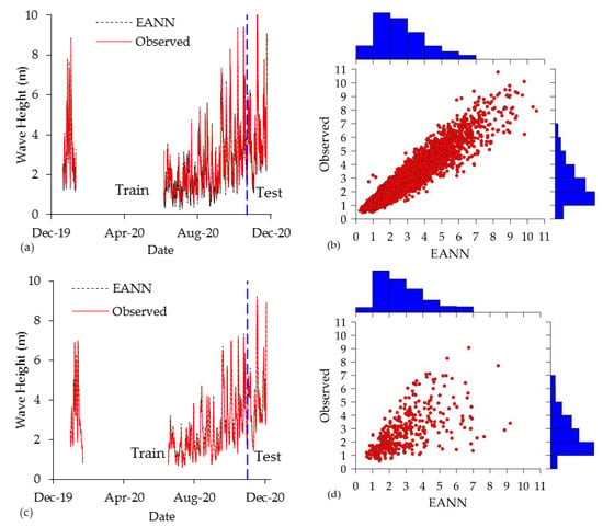
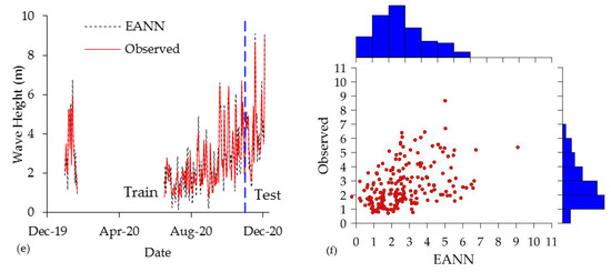
Figure 6.
A comparison of the wave height data for Buoy 46070 in Aleutian Basin with the prediction results of EANN model, (a,b) hourly wave data, (c,d) 12 h average wave data, and (e,f) daily wave data.
The comparison shown in Figure 7 is between the results calculated by the EANN model and the buoy wave height data collected by Buoy 42003 (Gulf of Mexico). In a manner similar to the findings concerning the Aleutian Basin, the EANN model performs significantly better when predicting hourly data in comparison to the 12 h average and daily data. However, this model demonstrates a performance that is satisfactory in predicting the maximum points in the time scales of the daily average and the 12 h average (Figure 6c,e and Figure 7c,e).
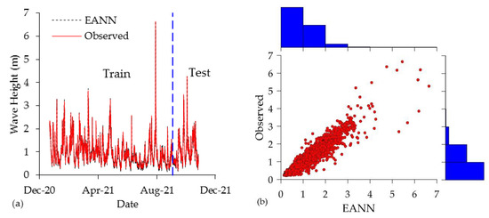
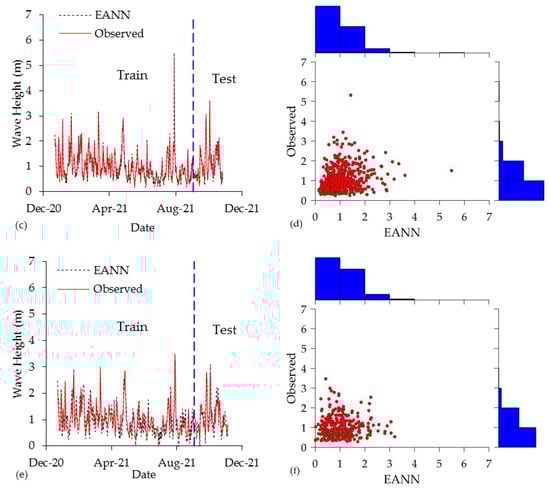
Figure 7.
A comparison of the wave height data for Buoy 42003 in Gulf of Mexico with the prediction results of EANN model, (a,b) hourly wave data, (c,d) 12 h average wave data, and (e,f) daily wave data.
In the Appendix A, a comparison between the simulation wave period and wave direction was made and is shown in Figure A3 and Figure A4 for both case studies. While previous studies [79] have demonstrated satisfactory performance of the EANN model in scenarios with scarce data, it is worth noting that the model’s performance has been observed to be superior in the hourly time scale when confronted with larger datasets, as compared to its performance in the 12 h average and daily time scales. However, previous research has confirmed that this model effectively captures peaks (Aleutian Basin wave height DCpeakHourly = 0.81 and Gulf of Mexico wave height DCpeakHourly = 0.79).
It seems that the EANN model has an adequate ability to predict the wave characteristics’ peak values. In contrast to the results of this model in hydrological studies, such as the rainfall-runoff model [80], the model did not perform well when trained with a small amount of data (daily time scale).
The utilization of shorter time steps as input data in the EANN model resulted in improved estimation accuracy and enhanced computational efficiency of the model; however, it increased the computational cost. The efficiency of the EANN model in handling limited data is a notable characteristic, as indicated by the findings of this study. However, it is important to note that the effectiveness of the model is contingent upon the quality of the input data and their temporal sequencing. Shorter time steps enhance the accuracy of the model in estimating wave characteristics despite the limited amount of available data. Based on the data collected from the studied areas, it can be concluded that the dispersion of the model output is ineffective in this particular case. The findings indicate that the model performs consistently in estimating wave characteristics across daily scale variations, regardless of the extent of the wave height range.
4.3. Wavelet Artificial Neural Network
The WANN model, which is capable of handling oscillation processes via multi-resolution wavelet analysis, was applied to hourly averages, 12 h averages, and daily time scale datasets. To improve the accuracy of modeling by WANN, preprocessed wavelet-based data were fed into the ANN. By separating the large and small features of a time series, the wavelet transform was used to process data at multiple time scales. The applied wavelet could decompose the input time series f(t) (as wave characteristics) or W(t) into one approximate subseries, fa(t) or Wa(t), and detailed subseries, fdl(t),..., fdi(t) or Wdl(t),..., Wdi(t) (i denotes the order of decomposition), such that each subseries could represent a distinct time scale of the seasonality involved in the time series. There exist numerous functions that can be associated with the characteristics of the primary time series in relation to the definition of a wavelet function. Based on prior research, Nourani et al. [81] found that the db4 mother wavelet is better suited. This is attributed to its greater resemblance to the signal and its ability to accurately capture the signal’s characteristics.
Table 4 presents the input parameters required to attain the optimal model for wave height estimation, based on case studies, for the purpose of selecting the most suitable network.
Table 4.
Results of WANN model for both Aleutian Basin and Gulf of Mexico Buoy dataset.
Figure 8 and Figure 9 depict the optimal model results derived from the validation data compared to Buoys 46070 and 42003, respectively. The results indicate that the WANN model demonstrated satisfactory performance in estimating a majority of the values, particularly with respect to the minimum and maximum values. The comparison between observed and simulated results of wave period and wave direction regarding Buoys 46070 and 42003 are shown in Figure A5 and Figure A6 in Appendix A.
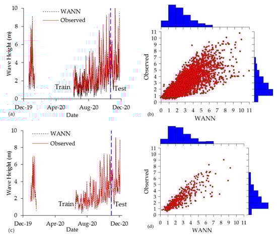
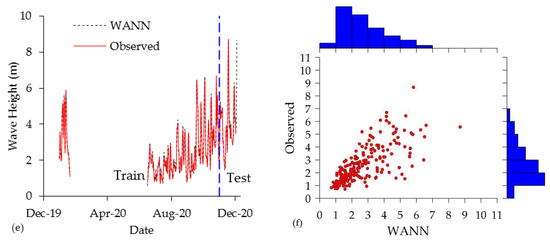
Figure 8.
A comparison of the wave height data for Buoy 46070 in Aleutian Basin with the prediction results of WANN model, (a,b) hourly wave data, (c,d) 12 h average wave data, and (e,f) daily wave data.
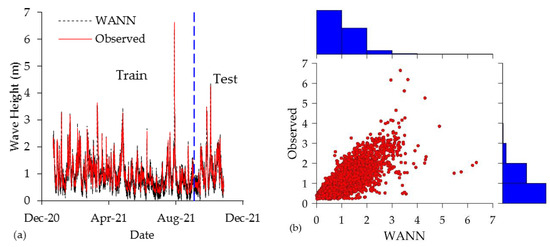
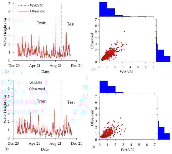
Figure 9.
A comparison of the wave height data for Buoy 42003 in Gulf of Mexico with the prediction results of WANN model, (a,b) hourly wave data, (c,d) 12 h average wave data, and (e,f) daily wave data.
As per the findings presented in Table 4, the WANN model exhibits superior performance in forecasting characteristic wave height for the 12 h average and daily time scales as compared to the hourly wave data. The present case has the potential to be interpreted similarly for both wave buoys.
The performance of the WANN model in predicting wave characteristics in both study areas demonstrates its effectiveness in capturing wave behavior over average 12 h and daily time scales. Nevertheless, the model’s performance exhibited superior results in the hourly time scale compared to the semi-analytical model. The NSE values for wave height prediction at the test phase of the WAAN hourly model are 0.3 and 0.73 for buoys 42003 and 47060, respectively. In contrast, for the SMB model, the NSE values are 0.11 and 0.50 for the same buoys and time scale.
4.4. Model Performance Comparison
Based on the findings outlined in the preceding sections, the current section will provide a comparative analysis of the SMB, EANN, and WANN models. The results indicate that the SMB model exhibits superior performance when applied to the daily dataset. Buoy 46070 exhibits t index indices of 91.62, 24.78, and 16.06 for the hourly, 12 h, and daily time scales, respectively. The SI index values for this particular case, as observed over the specified time scales, are 0.68, 0.45, and 0.32, respectively. In the case of Buoy 42003, the SMB model demonstrates better efficacy when implemented on the daily dataset. The t index values are 94.39, 27.62, and 19.09 for the hourly, 12 h, and daily time scales, respectively. The respective SI index values are 0.41, 0.40, and 0.33. Based on the findings of this study and the research conducted by Soomere [37], it can be inferred that SMB models continue to serve as effective tools for rapidly estimating specific features of wave climate at distinct locations.
The findings indicate that the EANN model exhibits satisfactory accuracy in forecasting wave height at an hourly temporal resolution for the specified research region. The t index values obtained during the test phase for the hourly time scale are 38.54, 99.37, and 57.45, respectively. Regarding the SI index, its values are 0.36, 0.73, and 0.73, in that order. The application of the EANN model demonstrates acceptable precision in predicting wave height at an hourly dataset for the designated regions in the Gulf of Mexico. The t index values acquired during the testing phase for the hourly, 12 h, and daily time scales are 32.78, 44.34, and 88.78, respectively. With respect to the SI index, the sequence of values is 0.92, 1.00, and 1.42.
Regarding the WANN model, it is noteworthy that out of the 46070 studies conducted, the model exhibited superior performance in the daily average time scale and 12 h average as compared to the hourly dataset. The t index values for the test stage of the model applied to the Buoy 46070 dataset at hourly, 12-hourly, and daily time scales are 141.84, 23.82, and 16.23, respectively. The performance of the model was evaluated for different time scales, namely the hourly average, 12 h average, and daily average time scales. The SI index values obtained for these time scales were 0.47, 0.37, and 0.37, respectively. The t index values obtained from the application of the WANN model to the Buoy 42003 dataset during the test stage, considering hourly, 12-hourly, and daily time scales, are 118.53, 40.13, and 22.22, respectively. The obtained SI index values for these specific time scales were 0.88, 0.79, and 0.84, respectively. The model’s performance was assessed across varying time scales, including the hourly average, 12 h average, and daily average time scales. These results suggest that the model exhibited superior performance in the 12 h average and daily average time scales.
The efficacy of the models to accurately capture the peak on the time series depends on the time scales and specific models employed. Nevertheless, the EANN model exhibited superior performance in capturing the peak of the time series when compared to the other two models. The EANN model demonstrates a performance of 0.82 and 0.88 on the hourly time scale, as measured by the DCpeak index, for the 42003 and 47060 buoys, respectively. Conversely, the WANN model exhibits its optimal performance on the 12 h time scale, with corresponding DCpeak index values for the 42003 and 47060 buoys yet to be specified by the value of 0.71 and 0.68, respectively. The semi-analytical model exhibits lower efficiency when compared to both machine learning models and the DCpeak index. Specifically, for Buoys 42003 and 47060, the DCpeak indices on a daily time scale are 0.55 and 0.54, respectively, for the SMB model. A similar pattern is observed in the parameters of the wave period, albeit with a minor distinction. Indeed, the ability to forecast peak values is a notable benefit of the EANN model, as it facilitates the estimation of wave power and energy.
The findings derived from this study exhibit conformity with the outcomes of Sharghi et al. [65]. The study conducted by Sharghi et al. [65] investigates the precision of two methodologies based on ANN for the purpose of modeling daily and monthly rainfall runoff. The researchers arrived at the conclusion that the EANN model is better suited for daily forecasting, whereas the WANN model exhibits superior performance in monthly modeling.
4.5. Wave Energy Density Spectrum
Corresponding to the preceding sections, ocean waves represent a renewable form of energy. Additionally, given the potential impact of wave energy on coastal structures, precise forecasting of ocean wave energy is crucial for the attainment of sustainability. The present study presents a comparison between the wave energy density spectrum obtained from the data of two case studies and the optimal outcomes of wave prediction through the utilization of the soft computing method, as illustrated in Figure 10. The findings indicate that the EANN approach exhibits superior concurrence in comparison to the WANN and SMB models in forecasting the wave energy density spectrum, particularly at the pinnacle juncture. This phenomenon is apparent in both areas of study. The aforementioned matter may be attributed to the utilization of wave data featuring an hourly temporal resolution within the context of the EANN model (Aleutian buoy (DCpeakEANN = 0.41) and Gulf of Mexico buoy (DCpeakEANN = 0.59)). In addition to accurately estimating the peak energy density, it is crucial to correctly estimate the peak frequency in the models. The aforementioned matter, particularly in offshore regions, exerts a substantial influence on the navigation of maritime vessels and their overall safety. Based on the findings pertaining to the energy spectrum density in both regions, it is evident that the EANN model not only demonstrates superior accuracy in estimating the peak of the wave energy spectrum, but also outperforms other models in accurately estimating the frequency corresponding to said wave energy peak.
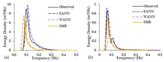
Figure 10.
The comparison between observed and machine learning estimation method wave energy density spectrum. (a) Buoy 46070 (Aleutian Basin) and (b) Buoy 42003 (Gulf of Mexico).
5. Conclusions
In this study, we proposed a novel approach for ocean wave forecasting that is based on semi-analytical and machine learning models. We applied this approach to a dataset of ocean wave measurements in two distinct case studies. The Aleutian Basin and Gulf of Mexico wave datasets were chosen as case studies. These regions are completely different in wave and climate conditions.
The present investigation assessed the efficacy of the SMB semi-analytical, EANN, and WANN methodologies for the estimation of ocean wave parameters. This study aimed to evaluate and compare the precision and dependability of different methodologies, as well as to examine the spatial and temporal fluctuations of the wave field. The aforementioned models are utilized to represent the non-linear associations between the input parameters and the output wave parameters, which are arduous to apprehend through conventional physical models. The study areas were evaluated using hourly and daily wave data for the purpose of model assessment. The results obtained from this research can be utilized to enhance the precision of wave prediction models and to facilitate the development of secure and effective marine infrastructures in the aforementioned areas.
Based on the outcomes, the SMB model shows t index values of 91.62, 24.78, and 16.06 for hourly, 12 h, and daily time scales, respectively, for the Aleutian Basin dataset. The corresponding SI index values are 0.68, 0.45, and 0.32. For the Gulf of Mexico dataset, the SMB model demonstrates better efficacy on the daily dataset with t index values of 94.39, 27.62, and 19.09 for hourly, 12 h, and daily time scales, respectively, and SI index values of 0.41, 0.40, and 0.33. The EANN model shows t index values of 38.54, 99.37, and 57.45, and SI index values of 0.36, 0.73, and 0.73 for hourly time scale, t index values of 32.78, 44.34, and 88.78, and SI index values of 0.92, 1.00, and 1.42 for hourly, 12 h, and daily time scales in the research region in the Gulf of Mexico, respectively. The WANN model exhibits superior performance in the daily and 12 h average time scales with t index values of 16.23 and 23.82 for the Aleutian Basin dataset and t index values of 22.22 and 40.13 for the Gulf of Mexico dataset. The corresponding SI index values are 0.37 and 0.47 for the Aleutian Basin dataset and 0.84 and 0.79 for the Buoy 42003 dataset. On the other hand, the results show that the SMB model performs better for daily datasets, while the EANN model is more accurate for hourly resolution for both case studies. However, the EANN model demonstrated satisfactory performance within the time scales of 12 and 24 h. The WANN model exhibits superior performance for daily and 12 h average time scales. Furthermore, the results related to the energy spectrum density indicate that the EANN model displays better performance when compared to other models, specifically in accurately predicting the spectrum’s peak.
However, the WANN model has adequate performance in all time scales and can be a suitable source for simulating sea waves. However, the SMB model performed better in predicting daily data. However, if there are hourly data, it is suggested to use the EANN model. This model also presented an acceptable performance in estimating the wave energy and estimated the maximum value of the spectrum better than other models.
According to the results, it is possible to use the WANN 12 h and daily model to predict the possibility of a tsunami occurring based on the predicted wave characteristics in order to reduce its potential risks to life in coastal zones. In actuality, the prediction is a step ahead of these models, particularly in terms of determining the direction of wave propagation; therefore, it is possible to predict the occurrence of unfortunate events. In contrast, due to its greater accuracy in predicting wave characteristics, the EANN hourly model can also be used in the marine transportation industry to estimate potential risks for maritime shipping and vessel pathways.
Author Contributions
Conceptualization, I.E.; methodology, I.E. and A.A.-M.; software, I.E. and S.H.A.; validation, A.A.; formal analysis, A.A.; investigation, S.H.A.; resources, A.A.; data curation, I.E. and A.A.-M.; writing—original draft preparation, A.A.-M; writing—review and editing, S.H.A.; visualization, A.A.-M. All authors have read and agreed to the published version of the manuscript.
Funding
The research was supported by the Deanship of Scientific Research at Najran University, Kingdom of Saudi Arabia.
Data Availability Statement
Not applicable.
Acknowledgments
The authors are thankful to the Deanship of Scientific Research at Najran University for funding this work, under the General Research Funding program grant code (NU/DRP/SERC/12/11).
Conflicts of Interest
The authors declare no conflict of interest.
Appendix A


Figure A1.
A comparison of the wave characteristic data for Buoy 46070 in Aleutian Basin with the prediction results of SMB model, (a) hourly wave period data, (b) 12 h average wave period data, (c) daily wave period data, (d) hourly wave direction data, (e) 12 h average wave direction data, and (f) daily wave direction data.


Figure A2.
A comparison of the wave characteristic data for Buoy 42003 in Gulf of Mexico with the prediction results of SMB model, (a) hourly wave period data, (b) 12 h average wave period data, (c) daily wave period data, (d) hourly wave direction data, (e) 12 h average wave direction data, and (f) daily wave direction data.


Figure A3.
A comparison of the wave characteristic data for Buoy 46070 in Aleutian Basin with the prediction results of EANN model, (a) hourly wave period data, (b) 12 h average wave period data, (c) daily wave period data, (d) hourly wave direction data, (e) 12 h average wave direction data, and (f) daily wave direction data.


Figure A4.
A comparison of the wave characteristic data for Buoy 42003 in Gulf of Mexico with the prediction results of EANN model, (a) hourly wave period data, (b) 12 h average wave period data, (c) daily wave period data, (d) hourly wave direction data, (e) 12 h average wave direction data, and (f) daily wave direction data.


Figure A5.
A comparison of the wave characteristic data for Buoy 46070 in Aleutian Basin with the prediction results of WANN model, (a) hourly wave period data, (b) 12 h average wave period data, (c) daily wave period data, (d) hourly wave direction data, (e) 12 h average wave direction data, and (f) daily wave direction data.


Figure A6.
A comparison of the wave characteristic data for Buoy 42003 in Gulf of Mexico with the prediction results of WANN model, (a) hourly wave period data, (b) 12 h average wave period data, (c) daily wave period data, (d) hourly wave direction data, (e) 12 h average wave direction data, and (f) daily wave direction data.
References
- Bateman, W.J.D.; Katsardi, V.; Swan, C. Extreme Ocean Waves. Part I. The Practical Application of Fully Nonlinear Wave Modelling. Appl. Ocean Res. 2012, 34, 209–224. [Google Scholar] [CrossRef]
- Golshani, A.; Banan-Dallalian, M.; Shokatian-Beiragh, M.; Samiee-Zenoozian, M.; Sadeghi-Esfahlani, S. Investigation of Waves Generated by Tropical Cyclone Kyarr in the Arabian Sea: An Application of ERA5 Reanalysis Wind Data. Atmosphere 2022, 13, 1914. [Google Scholar] [CrossRef]
- Mojtahedi, A.; Beiragh, M.S.; Farajpour, I.; Mohammadian, M. Investigation on Hydrodynamic Performance of an Environmentally Friendly Pile Breakwater. Ocean Eng. 2020, 217, 107942. [Google Scholar] [CrossRef]
- Zhao, L.; Li, Z.; Zhang, J.; Teng, B. An Integrated Complete Ensemble Empirical Mode Decomposition with Adaptive Noise to Optimize LSTM for Significant Wave Height Forecasting. J. Mar. Sci. Eng. 2023, 11, 435. [Google Scholar] [CrossRef]
- Yin, Y.; Le Guen, V.; Dona, J.; de Bézenac, E.; Ayed, I.; Thome, N.; Gallinari, P. Augmenting Physical Models with Deep Networks for Complex Dynamics Forecasting. J. Stat. Mech. Theory Exp. 2021, 2021, 124012. [Google Scholar] [CrossRef]
- Sadeghifar, T.; Lama, G.F.C.; Sihag, P.; Bayram, A.; Kisi, O. Wave Height Predictions in Complex Sea Flows through Soft-Computing Models: Case Study of Persian Gulf. Ocean Eng. 2022, 245, 110467. [Google Scholar] [CrossRef]
- Wu, L.; Breivik, Ø.; Rutgersson, A. Ocean-Wave-Atmosphere Interaction Processes in a Fully Coupled Modeling System. J. Adv. Model. Earth Syst. 2019, 11, 3852–3874. [Google Scholar] [CrossRef]
- Chaichitehrani, N.; Allahdadi, M.N.; Li, C. Simulation of Low Energy Waves during Fair-Weather Summer Conditions in the Northern Gulf of Mexico: Effect of Whitecapping Dissipation and the Forcing Accuracy. Atmosphere 2022, 13, 2047. [Google Scholar] [CrossRef]
- McPhaden, M.J.; Santoso, A.; Cai, W. Introduction to El Niño Southern Oscillation in a Changing Climate. In Geophysical Monograph Series; Wiley Online Library: Hoboken, NJ, USA, 2020; pp. 1–19. [Google Scholar]
- Wang, P.; Tian, X.; Peng, T.; Luo, Y. A Review of the State-of-the-Art Developments in the Field Monitoring of Offshore Structures. Ocean Eng. 2018, 147, 148–164. [Google Scholar] [CrossRef]
- Davidson, F.; Alvera-Azcárate, A.; Barth, A.; Brassington, G.B.; Chassignet, E.P.; Clementi, E.; De Mey-Frémaux, P.; Divakaran, P.; Harris, C.; Hernandez, F.; et al. Synergies in Operational Oceanography: The Intrinsic Need for Sustained Ocean Observations. Front. Mar. Sci. 2019, 6, 450. [Google Scholar] [CrossRef]
- Remya, P.G.; Rabi Ranjan, T.; Sirisha, P.; Harikumar, R.; Balakrishnan Nair, T.M. Indian Ocean Wave Forecasting System for Wind Waves: Development and Its Validation. J. Oper. Oceanogr. 2022, 15, 1–16. [Google Scholar] [CrossRef]
- Tajfar, I.; Pazoki, M.; Pazoki, A.; Nejatian, N.; Amiri, M. Analysis of Heating Value of Hydro-Char Produced by Hydrothermal Carbonization of Cigarette Butts. Pollution 2023, 9, 1273–1280. [Google Scholar] [CrossRef]
- Bento, P.M.R.; Pombo, J.A.N.; Mendes, R.P.G.; Calado, M.R.A.; Mariano, S.J.P.S. Ocean Wave Energy Forecasting Using Optimised Deep Learning Neural Networks. Ocean Eng. 2021, 219, 108372. [Google Scholar] [CrossRef]
- Chen, T.-C.; Najat Rashid, Z.; Theruvil Sayed, B.; Sari, A.; Kateb Jumaah Al-Nussairi, A.; Samiee-Zenoozian, M.; Shokatian-Beiragh, M. Evaluation of Hybrid Soft Computing Model’s Performance in Estimating Wave Height. Adv. Civ. Eng. 2023, 2023, 8272566. [Google Scholar] [CrossRef]
- Squire, V.A. Ocean Wave Interactions with Sea Ice: A Reappraisal. Annu. Rev. Fluid Mech. 2020, 52, 37–60. [Google Scholar] [CrossRef]
- Muscarella, P.; Brunner, K.; Walker, D. Estimating Coastal Winds by Assimilating High-Frequency Radar Spectrum Data in SWAN. Sensors 2021, 21, 7811. [Google Scholar] [CrossRef]
- Ali, M.; Prasad, R. Significant Wave Height Forecasting via an Extreme Learning Machine Model Integrated with Improved Complete Ensemble Empirical Mode Decomposition. Renew. Sustain. Energy Rev. 2019, 104, 281–295. [Google Scholar] [CrossRef]
- Silam Siregar, G.R.; Alfarizi, H.; Purnomo, F.M.; Ginanjar, S.; Wirasatriya, A. Validation of Wave Forecasting with the Sverdrup, Munk, and Bretschneider (SMB) Method Using Easywave Algorithm. In Proceedings of the 2020 IEEE Asia-Pacific Conference on Geoscience, Electronics and Remote Sensing Technology (AGERS), Jakarta, Indonesia, 7–8 December 2020; pp. 11–15. [Google Scholar]
- Benetazzo, A.; Barbariol, F.; Davison, S. Short-Term/Range Extreme-Value Probability Distributions of Upper Bounded Space-Time Maximum Ocean Waves. J. Mar. Sci. Eng. 2020, 8, 679. [Google Scholar] [CrossRef]
- Rahimian, M.; Beyramzadeh, M.; Siadatmousavi, S.M.; Allahdadi, M.N. Simulating Meteorological and Water Wave Characteristics of Cyclone Shaheen. Atmosphere 2023, 14, 533. [Google Scholar] [CrossRef]
- Ramos, M.S.; Farina, L.; Faria, S.H.; Li, C. Relationships between Large-Scale Climate Modes and the South Atlantic Ocean Wave Climate. Prog. Oceanogr. 2021, 197, 102660. [Google Scholar] [CrossRef]
- Li, M.; Liu, K. Probabilistic Prediction of Significant Wave Height Using Dynamic Bayesian Network and Information Flow. Water 2020, 12, 2075. [Google Scholar] [CrossRef]
- Banan-Dallalian, M.; Shokatian-Beiragh, M.; Golshani, A.; Mojtahedi, A.; Lotfollahi-Yaghin, M.A.; Akib, S. Study of the Effect of an Environmentally Friendly Flood Risk Reduction Approach on the Oman Coastlines during the Gonu Tropical Cyclone (Case Study: The Coastline of Sur). Eng 2021, 2, 141–155. [Google Scholar] [CrossRef]
- Gao, J.; Ji, C.; Gaidai, O.; Liu, Y. Numerical Study of Infragravity Waves Amplification during Harbor Resonance. Ocean Eng. 2016, 116, 90–100. [Google Scholar] [CrossRef]
- Gao, J.; Shi, H.; Zang, J.; Liu, Y. Mechanism Analysis on the Mitigation of Harbor Resonance by Periodic Undulating Topography. Ocean Eng. 2023, 281, 114923. [Google Scholar] [CrossRef]
- Gao, J.; Ma, X.; Dong, G.; Chen, H.; Liu, Q.; Zang, J. Investigation on the Effects of Bragg Reflection on Harbor Oscillations. Coast. Eng. 2021, 170, 103977. [Google Scholar] [CrossRef]
- Gao, J.; Zhou, X.; Zhou, L.; Zang, J.; Chen, H. Numerical Investigation on Effects of Fringing Reefs on Low-Frequency Oscillations within a Harbor. Ocean Eng. 2019, 172, 86–95. [Google Scholar] [CrossRef]
- Wang, J.; Shen, Y. Development and Validation of a Three-Dimensional, Wave-Current Coupled Model on Unstructured Meshes. Sci. China Phys. Mech. Astron. 2011, 54, 42–58. [Google Scholar] [CrossRef]
- Kim, S.; Barth, J.A. Connectivity and Larval Dispersal along the Oregon Coast Estimated by Numerical Simulations. J. Geophys. Res. 2011, 116, C06002. [Google Scholar] [CrossRef]
- Meng, Z.; Hu, Y.; Ancey, C. Using a Data Driven Approach to Predict Waves Generated by Gravity Driven Mass Flows. Water 2020, 12, 600. [Google Scholar] [CrossRef]
- Liu, F.; Chao, J.; Huang, G.; Feng, L. A Semi-Analytical Model for the Propagation of Rossby Waves in Slowly Varying Flow. Chin. Sci. Bull. 2011, 56, 2727–2731. [Google Scholar] [CrossRef][Green Version]
- Alifdini, I.; Sugianto, D.N.; Andrawina, Y.O.; Widodo, A.B. Identification of Wave Energy Potential with Floating Oscillating Water Column Technology in Pulau Baai Beach, Bengkulu. IOP Conf. Ser. Earth Environ. Sci. 2017, 55, 012040. [Google Scholar] [CrossRef]
- Young, I.R. Wind Generated Ocean Waves; Elsevier: Amsterdam, The Netherlands, 1999; ISBN 978-0-08-043317-2. [Google Scholar]
- Joensen, B.; Niclasen, B.A.; Bingham, H.B. Wave Power Assessment in Faroese Waters Using an Oceanic to Nearshore Scale Spectral Wave Model. Energy 2021, 235, 121404. [Google Scholar] [CrossRef]
- Akpinar, A.; Özger, M.; Bekiroglu, S.; Komurcu, M.I. Performance Evaluation of Parametric Models in the Hindcasting of Wave Parameters along the South Coast of Black Sea. Indian J. Geo-Mar. Sci. 2014, 43, 899–914. [Google Scholar]
- Soomere, T. Numerical Simulations of Wave Climate in the Baltic Sea: A Review. Oceanologia 2023, 65, 117–140. [Google Scholar] [CrossRef]
- Bishop, C.T. Comparison of Manual Wave Prediction Models. J. Waterw. Port Coast. Ocean Eng. 1983, 109, 1–17. [Google Scholar] [CrossRef]
- Malekmohamadi, I.; Bazargan-Lari, M.R.; Kerachian, R.; Nikoo, M.R.; Fallahnia, M. Evaluating the Efficacy of SVMs, BNs, ANNs and ANFIS in Wave Height Prediction. Ocean Eng. 2011, 38, 487–497. [Google Scholar] [CrossRef]
- Chang, H.-K.; Liou, J.-C.; Liu, S.-J.; Liaw, S.-R. Simulated Wave-Driven ANN Model for Typhoon Waves. Adv. Eng. Softw. 2011, 42, 25–34. [Google Scholar] [CrossRef]
- Suursaar, Ü. Locally Calibrated Wave Hindcasts in the Estonian Coastal Sea in 1966–2011. Est. J. Earth Sci. 2013, 62, 42–56. [Google Scholar] [CrossRef]
- Suursaar, Ü.; Jaagus, J.; Tõnisson, H. How to Quantify Long-Term Changes in Coastal Sea Storminess? Estuar. Coast. Shelf Sci. 2015, 156, 31–41. [Google Scholar] [CrossRef]
- Domala, V.; Lee, W.; Kim, T. Wave Data Prediction with Optimized Machine Learning and Deep Learning Techniques. J. Comput. Des. Eng. 2022, 9, 1107–1122. [Google Scholar] [CrossRef]
- Zhang, J.; Zhao, X.; Jin, S.; Greaves, D. Phase-Resolved Real-Time Ocean Wave Prediction with Quantified Uncertainty Based on Variational Bayesian Machine Learning. Appl. Energy 2022, 324, 119711. [Google Scholar] [CrossRef]
- den Bieman, J.P.; van Gent, M.R.A.; van den Boogaard, H.F.P. Wave Overtopping Predictions Using an Advanced Machine Learning Technique. Coast. Eng. 2021, 166, 103830. [Google Scholar] [CrossRef]
- Fan, S.; Xiao, N.; Dong, S. A Novel Model to Predict Significant Wave Height Based on Long Short-Term Memory Network. Ocean Eng. 2020, 205, 107298. [Google Scholar] [CrossRef]
- Dai, H.; Shang, S.; Lei, F.; Liu, K.; Zhang, X.; Wei, G.; Xie, Y.; Yang, S.; Lin, R.; Zhang, W. CRBM-DBN-Based Prediction Effects Inter-Comparison for Significant Wave Height with Different Patterns. Ocean Eng. 2021, 236, 109559. [Google Scholar] [CrossRef]
- Londhe, S.N.; Shah, S.; Dixit, P.R.; Nair, T.M.B.; Sirisha, P.; Jain, R. A Coupled Numerical and Artificial Neural Network Model for Improving Location Specific Wave Forecast. Appl. Ocean Res. 2016, 59, 483–491. [Google Scholar] [CrossRef]
- James, S.C.; Zhang, Y.; O’Donncha, F. A Machine Learning Framework to Forecast Wave Conditions. Coast. Eng. 2018, 137, 1–10. [Google Scholar] [CrossRef]
- Tsai, C.-P.; Lin, C.; Shen, J.-N. Neural Network for Wave Forecasting among Multi-Stations. Ocean Eng. 2002, 29, 1683–1695. [Google Scholar] [CrossRef]
- Makarynskyy, O.; Pires-Silva, A.A.; Makarynska, D.; Ventura-Soares, C. Artificial Neural Networks in Wave Predictions at the West Coast of Portugal. Comput. Geosci. 2005, 31, 415–424. [Google Scholar] [CrossRef]
- Gopinath, D.I.; Dwarakish, G.S. Wave Prediction Using Neural Networks at New Mangalore Port along West Coast of India. Aquat. Procedia 2015, 4, 143–150. [Google Scholar] [CrossRef]
- Ahn, H.; Kim, K. Bankruptcy Prediction Modeling with Hybrid Case-Based Reasoning and Genetic Algorithms Approach. Appl. Soft Comput. 2009, 9, 599–607. [Google Scholar] [CrossRef]
- Dixit, P.; Londhe, S.N.; Dandawate, Y.H. Wave Forecasting Using Neuro Wavelet Technique. Int. J. Ocean Clim. Syst. 2014, 5, 237–247. [Google Scholar] [CrossRef][Green Version]
- Sharghi, E.; Nourani, V.; Najafi, H.; Gokcekus, H. Conjunction of a Newly Proposed Emotional ANN (EANN) and Wavelet Transform for Suspended Sediment Load Modeling. Water Sci. Technol. Water Supply 2019, 19, 1726–1734. [Google Scholar] [CrossRef]
- Nourani, V.; Molajou, A.; Uzelaltinbulat, S.; Sadikoglu, F. Emotional Artificial Neural Networks (EANNs) for Multi-Step Ahead Prediction of Monthly Precipitation; Case Study: Northern Cyprus. Theor. Appl. Climatol. 2019, 138, 1419–1434. [Google Scholar] [CrossRef]
- Nourani, V.; Molajou, A.; Najafi, H.; Danandeh Mehr, A. Emotional ANN (EANN): A New Generation of Neural Networks for Hydrological Modeling in IoT. In Artificial Intelligence in IoT; Springer: Cham, Switzerland, 2019; pp. 45–61. [Google Scholar]
- Danielson, S.L.; Ahkinga, O.; Ashjian, C.; Basyuk, E.; Cooper, L.W.; Eisner, L.; Farley, E.; Iken, K.B.; Grebmeier, J.M.; Juranek, L.; et al. Manifestation and Consequences of Warming and Altered Heat Fluxes over the Bering and Chukchi Sea Continental Shelves. Deep Sea Res. Part II Top. Stud. Oceanogr. 2020, 177, 104781. [Google Scholar] [CrossRef]
- Danielson, S.L.; Weingartner, T.J.; Hedstrom, K.S.; Aagaard, K.; Woodgate, R.; Curchitser, E.; Stabeno, P.J. Coupled Wind-Forced Controls of the Bering–Chukchi Shelf Circulation and the Bering Strait Throughflow: Ekman Transport, Continental Shelf Waves, and Variations of the Pacific–Arctic Sea Surface Height Gradient. Prog. Oceanogr. 2014, 125, 40–61. [Google Scholar] [CrossRef]
- Katsuki, K.; Khim, B.-K.; Itaki, T.; Harada, N.; Sakai, H.; Ikeda, T.; Takahashi, K.; Okazaki, Y.; Asahi, H. Land—Sea Linkage of Holocene Paleoclimate on the Southern Bering Continental Shelf. Holocene 2009, 19, 747–756. [Google Scholar] [CrossRef]
- Roden, G.I. Aleutian Basin of the Bering Sea: Thermohaline, Oxygen, Nutrient, and Current Structure in July 1993. J. Geophys. Res. 1995, 100, 13539. [Google Scholar] [CrossRef]
- Sallenger, A.H., Jr. Storm Impact Scale for Barrier Islands. J. Coast. Res. 2000, 16, 890–895. [Google Scholar]
- Sheng, Y.P.; Zhang, Y.; Paramygin, V.A. Simulation of Storm Surge, Wave, and Coastal Inundation in the Northeastern Gulf of Mexico Region during Hurricane Ivan in 2004. Ocean Model. 2010, 35, 314–331. [Google Scholar] [CrossRef]
- Harris, C.; Syvitski, J.; Arango, H.G.; Meiburg, E.H.; Cohen, S.; Jenkins, C.J.; Birchler, J.; Hutton, E.W.H.; Kniskern, T.A.; Radhakrishnan, S.; et al. Data-Driven, Multi-Model Workflow Suggests Strong Influence from Hurricanes on the Generation of Turbidity Currents in the Gulf of Mexico. J. Mar. Sci. Eng. 2020, 8, 586. [Google Scholar] [CrossRef]
- Sharghi, E.; Nourani, V.; Najafi, H.; Molajou, A. Emotional ANN (EANN) and Wavelet-ANN (WANN) Approaches for Markovian and Seasonal Based Modeling of Rainfall-Runoff Process. Water Resour. Manag. 2018, 32, 3441–3456. [Google Scholar] [CrossRef]
- Molajou, A.; Nourani, V.; Afshar, A.; Khosravi, M.; Brysiewicz, A. Optimal Design and Feature Selection by Genetic Algorithm for Emotional Artificial Neural Network (EANN) in Rainfall-Runoff Modeling. Water Resour. Manag. 2021, 35, 2369–2384. [Google Scholar] [CrossRef]
- Haruna, S.I.; Malami, S.I.; Adamu, M.; Usman, A.G.; Farouk, A.; Ali, S.I.A.; Abba, S.I. Compressive Strength of Self-Compacting Concrete Modified with Rice Husk Ash and Calcium Carbide Waste Modeling: A Feasibility of Emerging Emotional Intelligent Model (EANN) Versus Traditional FFNN. Arab. J. Sci. Eng. 2021, 46, 11207–11222. [Google Scholar] [CrossRef]
- Sharghi, E.; Paknezhad, N.J.; Najafi, H. Assessing the Effect of Emotional Unit of Emotional ANN (EANN) in Estimation of the Prediction Intervals of Suspended Sediment Load Modeling. Earth Sci. Inform. 2021, 14, 201–213. [Google Scholar] [CrossRef]
- Yadav, A.; Chithaluru, P.; Singh, A.; Joshi, D.; Elkamchouchi, D.; Pérez-Oleaga, C.; Anand, D. An Enhanced Feed-Forward Back Propagation Levenberg–Marquardt Algorithm for Suspended Sediment Yield Modeling. Water 2022, 14, 3714. [Google Scholar] [CrossRef]
- Farooq, M.U.; Zafar, A.M.; Raheem, W.; Jalees, M.I.; Aly Hassan, A. Assessment of Algorithm Performance on Predicting Total Dissolved Solids Using Artificial Neural Network and Multiple Linear Regression for the Groundwater Data. Water 2022, 14, 2002. [Google Scholar] [CrossRef]
- Zuccaro, G.; Leone, M.F.; Zuber, S.Z.; Nawi, M.N.M.; Nifa, F.A.; Zou, Y.; Kiviniemi, A.; Jones, S.W.; Zou, P.X.W.; Lun, P.; et al. Productivity of Digital Fabrication in Construction: Cost and Time Analysis of a Robotically Built Wall. Autom. Constr. 2019, 92, 297–311. [Google Scholar]
- Tariq, R.; Alhamrouni, I.; Rehman, A.U.; Tag Eldin, E.; Shafiq, M.; Ghamry, N.A.; Hamam, H. An Optimized Solution for Fault Detection and Location in Underground Cables Based on Traveling Waves. Energies 2022, 15, 6468. [Google Scholar] [CrossRef]
- Qin, Y.; Tang, B.; Wang, J. Higher-Density Dyadic Wavelet Transform and Its Application. Mech. Syst. Signal Process. 2010, 24, 823–834. [Google Scholar] [CrossRef]
- Nourani, V.; Molajou, A.; Tajbakhsh, A.D.; Najafi, H. A Wavelet Based Data Mining Technique for Suspended Sediment Load Modeling. Water Resour. Manag. 2019, 33, 1769–1784. [Google Scholar] [CrossRef]
- Dixit, P.; Londhe, S. Prediction of Extreme Wave Heights Using Neuro Wavelet Technique. Appl. Ocean Res. 2016, 58, 241–252. [Google Scholar] [CrossRef]
- Saber, A.; James, D.E.; Hayes, D.F. Long-term Forecast of Water Temperature and Dissolved Oxygen Profiles in Deep Lakes Using Artificial Neural Networks Conjugated with Wavelet Transform. Limnol. Oceanogr. 2020, 65, 1297–1317. [Google Scholar] [CrossRef]
- Jacovides, C.P. Model Comparison for the Calculation of Linke’s Turbidity Factor. Int. J. Climatol. 1997, 17, 551–563. [Google Scholar] [CrossRef]
- Wang, N.; Chen, Q.; Zhu, L.; Sun, H. Integration of Data-Driven and Physics-Based Modeling of Wind Waves in a Shallow Estuary. Ocean Model. 2022, 172, 101978. [Google Scholar] [CrossRef]
- Nourani, V. An Emotional ANN (EANN) Approach to Modeling Rainfall-Runoff Process. J. Hydrol. 2017, 544, 267–277. [Google Scholar] [CrossRef]
- Sharghi, E.; Nourani, V.; Molajou, A.; Najafi, H. Conjunction of Emotional ANN (EANN) and Wavelet Transform for Rainfall-Runoff Modeling. J. Hydroinform. 2019, 21, 136–152. [Google Scholar] [CrossRef]
- Nourani, V.; Hosseini Baghanam, A.; Adamowski, J.; Kisi, O. Applications of Hybrid Wavelet–Artificial Intelligence Models in Hydrology: A Review. J. Hydrol. 2014, 514, 358–377. [Google Scholar] [CrossRef]
Disclaimer/Publisher’s Note: The statements, opinions and data contained in all publications are solely those of the individual author(s) and contributor(s) and not of MDPI and/or the editor(s). MDPI and/or the editor(s) disclaim responsibility for any injury to people or property resulting from any ideas, methods, instructions or products referred to in the content. |
© 2023 by the authors. Licensee MDPI, Basel, Switzerland. This article is an open access article distributed under the terms and conditions of the Creative Commons Attribution (CC BY) license (https://creativecommons.org/licenses/by/4.0/).