1. Introduction
Ocean wave energy conversion systems are devices that include buoys, generators, and other auxiliary parts [
1,
2]. Depending on the different types of system design, ocean wave energy conversion systems are usually fixed on the shoreline, installed near the shore, or placed in offshore locations [
3,
4,
5]. Under the buoyancy-driven action of ocean waves, the ocean wave energy conversion system buoy experiences motion, which then drives the generator to convert ocean wave energy into electrical energy.
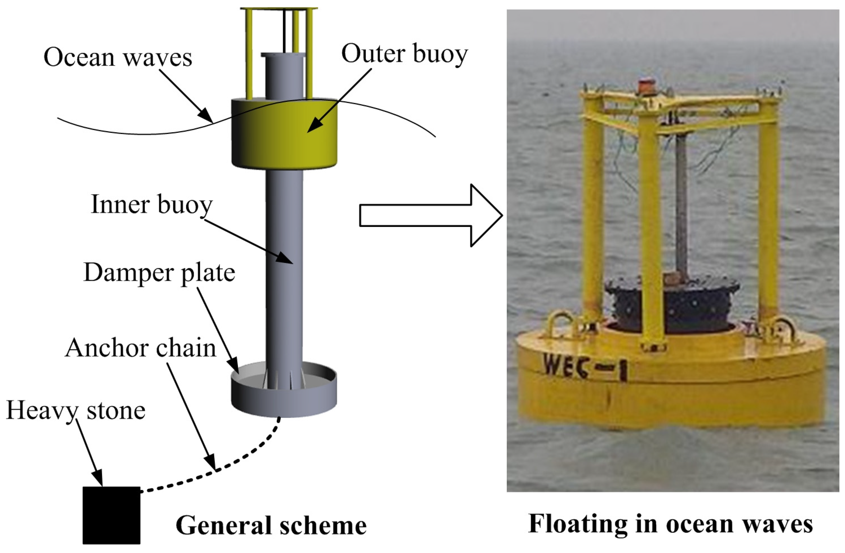
Figure 1 shows one type of ocean wave energy converter, which is placed in offshore locations. According to the motion characteristics of ocean waves, the deeper the water, the smaller the vertical direction motion amplitude. Therefore, differences in draught lead to a relative vertical direction motion between the outer buoy and inner buoy, which drives the linear generator (installed in the upper end of inner buoy) to convert ocean wave energy into electrical energy [
6]. More details about the motion characteristics of buoys in ocean waves and the operation principle of the offshore type of ocean wave energy converter can be found in previous studies [
7,
8,
9].
Under natural conditions, the operational efficiency of an ocean wave energy conversion system is low [
10]. Therefore, in addition to structure optimization measures such as changes to buoy and generator design, optimization control technology is also an effective method for improving the operational efficiency of ocean wave energy conversion systems, allowing the maximization of the energy conversion from ocean wave energy into electrical energy. Specifically, the purpose of optimization control technology is to achieve resonant motion (or synchronous motion) between the ocean wave height and the buoy of ocean wave energy conversion system. When resonant motion occurs, the efficiency of the wave energy conversion system can be improved [
11].
Based on the ocean wave height, some optimization control methods were investigated by simulation analysis or hardware experiments, with the aim of improving the operational efficiency of ocean wave energy conversion systems. In 2016, a novel unconstrained control method for a WEC (wave energy converter) considering the iteration between geometry optimization and control technology design was studied by Paula et al. [
12]. The simulation results showed that the efficiency of the WEC could be increased significantly only when the matching relationship between the system geometries (when the system’s nature frequency is consistent with the frequency of the ocean waves) and the control technology design are considered comprehensively. In 2020, Violini et al. proposed an LTI (linear time invariant) control method for the improvement of the efficiency of a WEC [
13]. In case of regular and irregular real ocean wave height, the comparison results between the LTI control method and existing control methods showed that the former method is preferred over the latter. In addition, researchers built a hardware platform of ocean wave energy conversion system, and the corresponding optimization control methods were tested [
14,
15]. In Zhang et al. [
14], an adaptive sliding mode control method containing a back-stepping strategy was proposed and applied on an experimental platform, and the advantages of this control method were verified by comparison with the PID control method. In Pei et al. [
15], an improved MPPT (Maximum Power Point Tracking) method of WEC was modeled and tested. After the experimental test (in different wave working conditions), the improved MPPT method was found to be better than the other control methods, and had the advantages of stability and high effectiveness.
An analysis of
Figure 1 and the above optimization control methods for ocean wave energy conversion systems demonstrated that predictions of future ocean wave height are beneficial to the improvement of the efficiency of ocean wave energy conversion systems. This is because the ultimate aim of optimization control of ocean wave energy conversion is to achieve resonant motion between the ocean wave height and the buoy of the ocean wave energy conversion system. This study draws upon the work of reference [
16], which proposed a method for decomposing the physical processes involved in Bragg reflection. Through a systematic analysis of the amplitude of sinusoidal bars and their optimal wavelength for achieving the best mitigation effect, this study offers valuable insights for predicting ocean wave fields. Additionally, reference [
17] introduces a wavelet neural network method aimed at enhancing the prediction accuracy of significant wave height and peak wave period in ocean waves. The research findings indicate that the suggested prediction method (wavelet neural network) is preferred over the standalone neural network method. In the context of a specific structure of an ocean wave energy conversion system (
Figure 1), accurate forecasting and confirmation of future ocean wave height within the 2~3 s range would facilitate the implementation of an optimized control process for the said energy conversion system.
The primary contributions of this paper can be summarized as follows. Firstly, an analysis of the real fluctuation characteristics of ocean wave height is conducted, and a denoising method is employed to enhance the smoothness of the ocean wave height time series. Secondly, three forecasting methods, namely the ARMA method, the BP neural network method and the RBF neural network method, are presented. Thirdly, a comparative analysis is performed to evaluate the forecast accuracy and computational time consumption of these three methods. Finally, the comparison results and subsequent discussions demonstrate that the RBF neural network method outperforms the other two forecasting methods, thereby enhancing the operational control and efficiency of ocean wave energy conversion system.
2. Denoising and Smoothing of Real Ocean Wave Height
In the real ocean environment, ocean waves exhibit nonlinearity, irregularity, and varying wave periods and heights [
18,
19].
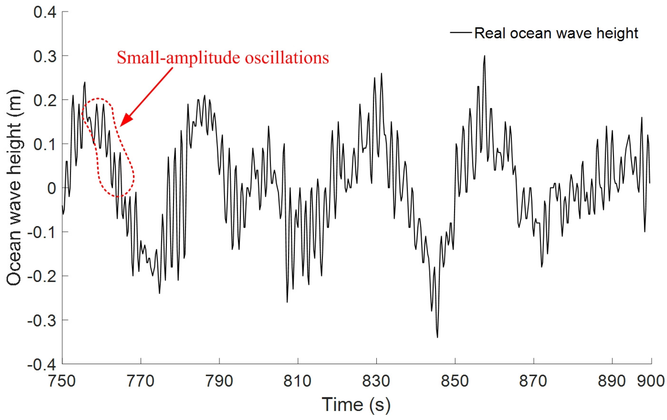
Figure 2 illustrates a time series of real ocean waves observed near Lianyungang port, in the Yellow Sea on 1 November 2017, using a buoy-type wave height measuring instrument. It is evident from
Figure 2 that real ocean waves are characterized by nonlinearity and irregularity, particularly the presence of small-amplitude oscillations. In such circumstances, effective and accurate forecasting of ocean wave height becomes challenging. Moreover, considering factors such as motion inertia, additional mass, damping coefficient, and natural frequency of the buoy in ocean waves, it can be inferred that small-amplitude oscillations do not significantly impact on the motion process of a buoy [
20,
21,
22]. For instance, if the horizontal diameter of the buoy exceeds the wavelength of the ocean waves by 0.2 times (as observed in the high-frequency and small-amplitude oscillations of ocean waves in
Figure 2), the buoy motion process remains largely unaffected [
23].
Therefore, prior to prognosticating future ocean wave height, it is necessary to preprocess the historical time series of ocean wave height with the objective of enhancing its fluidity.
This paper adopts the frequency domain method of the Butterworth filter to achieve the denoising and smoothing of real ocean wave height [
24,
25]. The transfer function (magnitude frequency response) of the Butterworth filter can be described as
where
represents nature frequency,
denotes corner frequency and
indicates system order. If the coefficient
, then the gain of Butterworth filter corresponding to the corner frequency
is −3 dB. In addition, with the system order of Butterworth filter increasing, the smooth of filtered curve of ocean wave height increases simultaneously.
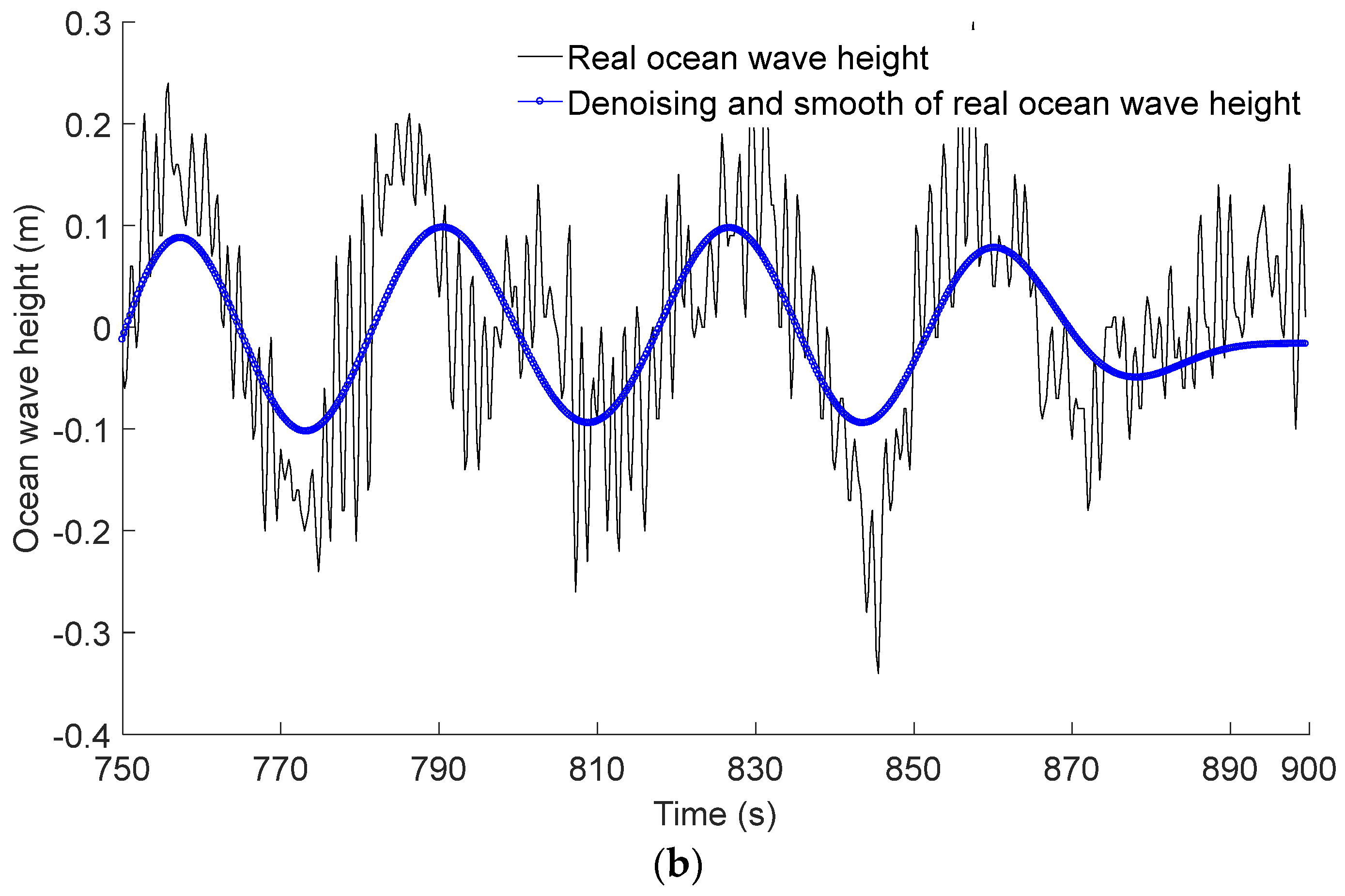
Figure 3a showcases the denoising result of real ocean wave height through the utilization of the Butterworth filter. In this instance, the natural frequency of the Butterworth filter is 0.02 × 2, the duration of the time series is 150 s (from the 750th s to the 900th s), and the temporal interval between adjacent data points of the real ocean wave height is 0.25 s.
Figure 3a signifies that subsequent to the denoising process, the ocean wave height attains a state of smoothness. In addition, during the denoising process, it is also observed that as the natural frequency of the Butterworth filter decreases, the filtered curve of the ocean wave height becomes increasingly smoother. However, if the natural frequency of the Butterworth filter is chosen imprudently, a severe distortion of the ocean wave height curve occurs, as depicted in
Figure 3b, where the natural frequency of the Butterworth filter is 0.0085 × 2. Therefore, a suitable selection of an appropriate natural frequency for the Butterworth filter is pivotal in ensuring the smoothness and non-distortion of the ocean wave height.
Several alternative methodologies can also be employed for the denoising and smoothing of real ocean wave height, including the polynomial function, the Chebyshev filter, and the finite impulse response filter, among others [
26,
27,
28].
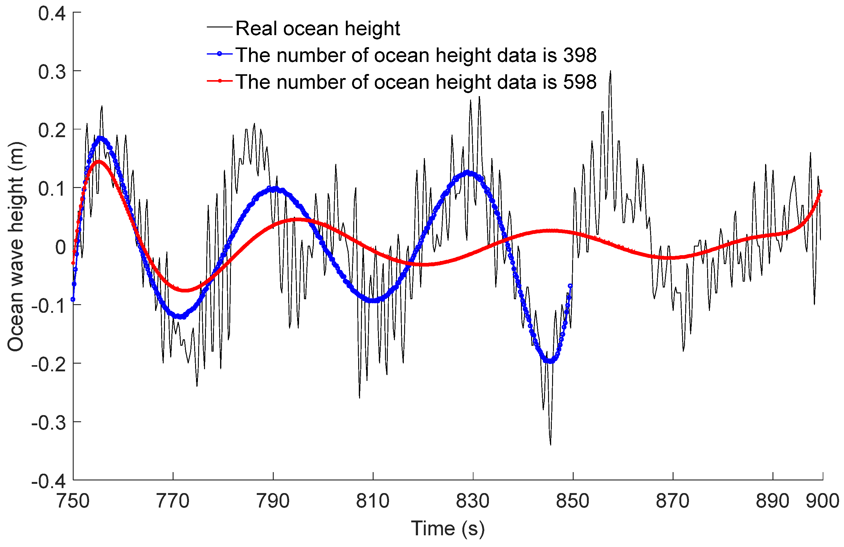
Figure 4 illustrates a time domain approach utilizing the polynomial function to denoise and smooth the real ocean wave height, with the polynomial function being of a ninth order. From
Figure 4, it can be deduced that an increased quantity of ocean wave height data leads to a greater degree of distortion in the ocean wave height. Therefore, when compared to the time domain method, the frequency domain method of denoising and smoothing ocean wave height possesses the advantages of precision and efficacy.
3. Forecasting Methods of Ocean Wave Height
Building upon the denoising and smoothing of real ocean wave height expounded upon in
Section 2, this subsequent section employs three methodologies, namely the ARMA method, the BP neural network method and the RBF neural network method to forecast the future ocean wave height.
3.1. ARMA Method
The basic expression of ARMA method can be written as
where
represents the forecasted data,
denotes time series of historical data,
indicates autoregressive coefficient,
signifies moving average coefficient and
expresses white noise sequence [
29].
Equation (2) indicates that the forecasted data are determined by the time series of historical data, autoregressive coefficient, moving average coefficient, and white noise sequence. Therefore, it is necessary to devise reasonable measures to enhance the feasibility and accuracy of ARMA method in forecasting the future ocean wave heights.
Firstly, the stationary analysis of the time series of historical data must be achieved. Only when the time series of historical data exhibits stationarity can the forecasted future data of ocean wave heights be deemed meaningful and accurate. This paper study employs differential calculation methods to eliminate the non-stationary of the time series of historical ocean wave heights.
Secondly, the orders
and
of Equation (2) necessitate determination and establishment. In actuality, appropriate orders are advantageous in striking a balance between computation time (the shorter the better) and forecast accuracy. This paper adopts the minimum value method of the Akaike information criterion (AIC) to select the suitable orders
and
and assesses the rationality of orders
and
by the truncation analysis of time series data. Taking the order
as an example, its AIC can be written as
In Equation (3), represents random error and denotes the number of time series. Under the condition that increases (the decreases concurrently), a minimum value of must occur. Therefore, parameter that corresponds to the minimum value of is the suitable order of Equation (2). In addition, during the process of forecasting real ocean wave heights using a computer program, the orders and should be slightly adjusted with the aim of reducing computation time and ensuring forecast accuracy.
Thirdly, based on the determined orders
and
, the parameters of Equation (2) such as the autoregressive coefficient
, moving average coefficient
and white noise sequence
can be estimated. The conventional methods for parameter estimation include matrix estimation, least square estimation and maximum likelihood estimation [
30,
31]. Many numerical computation software packages employ the least square estimation method to establish the parameters estimation for the ARMA method.
Lastly, the ARMA method is constructed, and the future data are calculated using the ARMA method.
3.2. BP Neural Network Method
In 1986, Rumelhart and McClelland proposed the preliminary framework of the BP neural network [
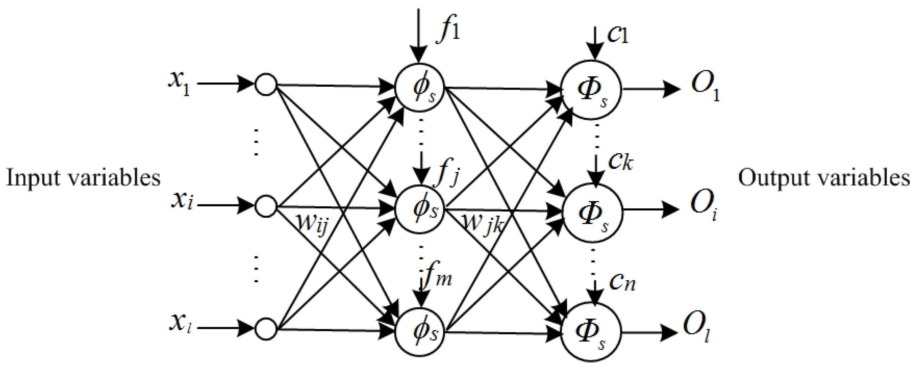
32]. After a series of advancements and refinements, the contemporary BP neural network comprises an input layer, a hidden layer and an output layer. With the characteristic of forward propagation of input variables and backward propagation of weights (thresholds), the BP neural network possesses the functions of data forecasting, pattern recognition, and type discrimination. Furthermore, it should be noted that the data forecasting function of the BP neural network is realized through the S-type neurons, which differs from the data fitting function (principle) of conventional forecasting methods.
Figure 5 shows a kind of BP neural network structure with one hidden layer. In
Figure 5,
represents the input variables,
denotes the weight value between the input layer and hidden layer,
signifies the threshold value of the hidden layer,
represents the S-type function (base function) of the hidden layer,
expresses the weight value between the hidden layer and the output layer,
indicates the threshold value of the output layer,
conveys the linear function of the output layer and
refers to the output variables.
The forward propagation equation of input variables of BP neural network can be described as
In Equation (4), the gradient method is employed to adjust the weight value (, ) and the threshold value (, ), thereby enabling the output variables to closely approximate the real value. Therefore, Equation (4) indicates the applicability of the BP neural network method in forecasting future ocean wave height.
3.3. RBF Neural Network Method
The initial prototype of the RBF neural network was proposed in the 1980s, and it can be utilized for the prediction of future time series data [
33]. The structure of the RBF neural network closely resembles that of the BP neural network, including an input layer, hidden layer and output layer. However, the RBF neural network adopts the OLS (orthogonal least square) method to adjust the weight value and other parameters while employing the Gaussian function as the basis function for the hidden layer.
The output of RBF neural network can be written as
where
represents the output variables,
denotes the weight value between the
node of the hidden layer and the
node of the output layer,
signifies the input variables,
denotes the center vector of the base function in the hidden layer, and
corresponds to the variance of the Gaussian function.
In Equation (5), the variance of the Gaussian function
significantly influences the forecast accuracy of RBF neural network. Therefore, this paper adopts the FOA (fruit fly optimization algorithm) to select parameter
[
34].
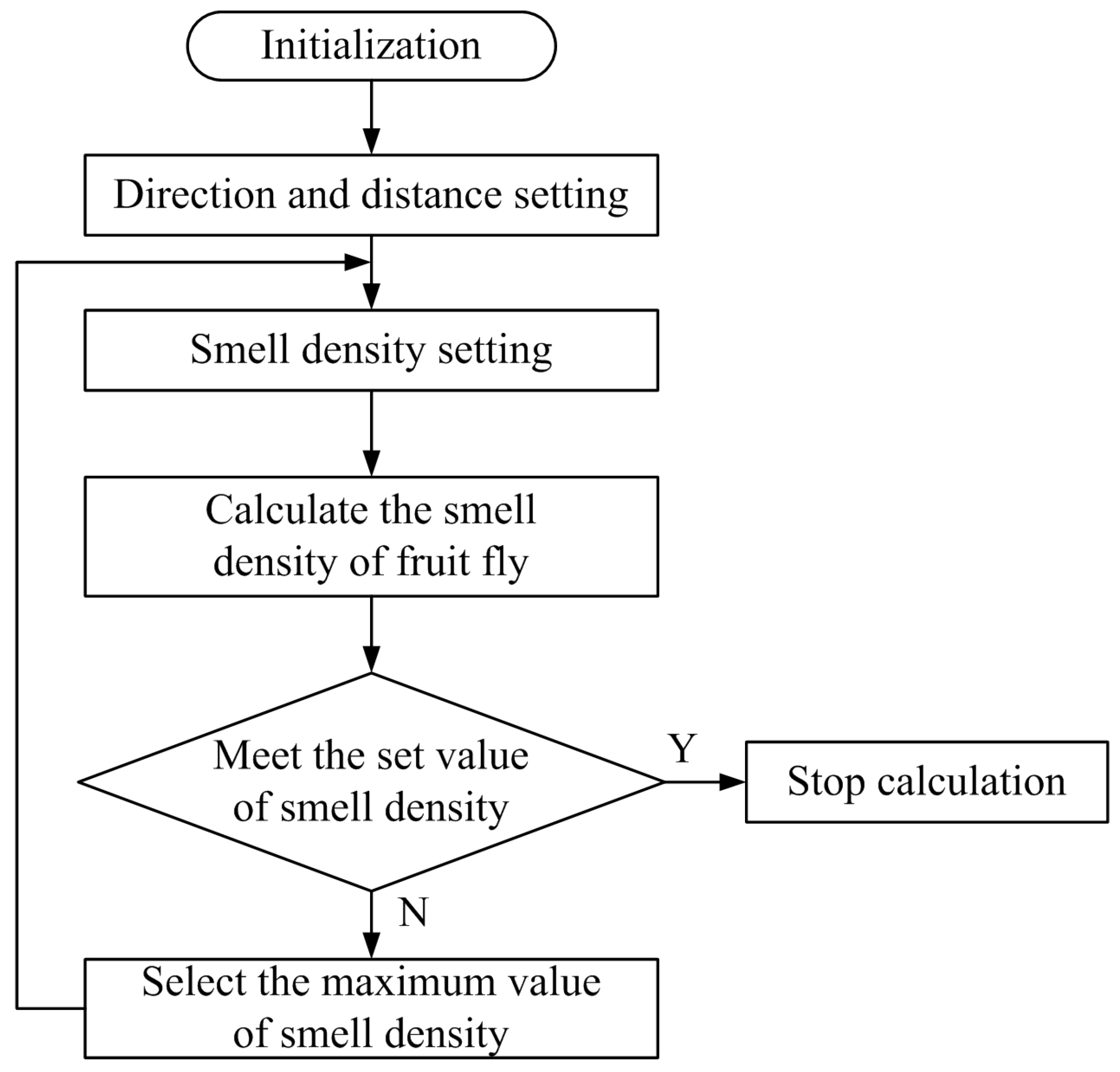
Figure 6 shows the data analysis and the process of the FOA. The flow of the FOA is as follows:
Step 1. Parameter initialization, such as the initial position of fruit flies and the maximum number of FOA iterations.
Step 2. Definition of the direction and distance for the food search of fruit flies.
Step 3. Under the normal condition, the setting of smell density to be determined by the reciprocal of the distance (between the fruit fly and the origin point).
Step 4. Calculation of the smell density for each fruit fly using the fitness function.
Step 5. When the calculated smell density of a fruit fly satisfies the smell density setting of Step 3, the data analysis and process of the FOA are terminated. Otherwise, the maximum value of the calculated smell density is selected, and the calculation process is repeated from Step 3 or the maximum number of iterations from Step 1.
4. Results and Comparison
After the mathematical model analysis of the ARMA method, the BP neural network method and the neural RBF network method, a future ocean wave height within a 2~3 s range was computed using the aforementioned three forecasting methods.
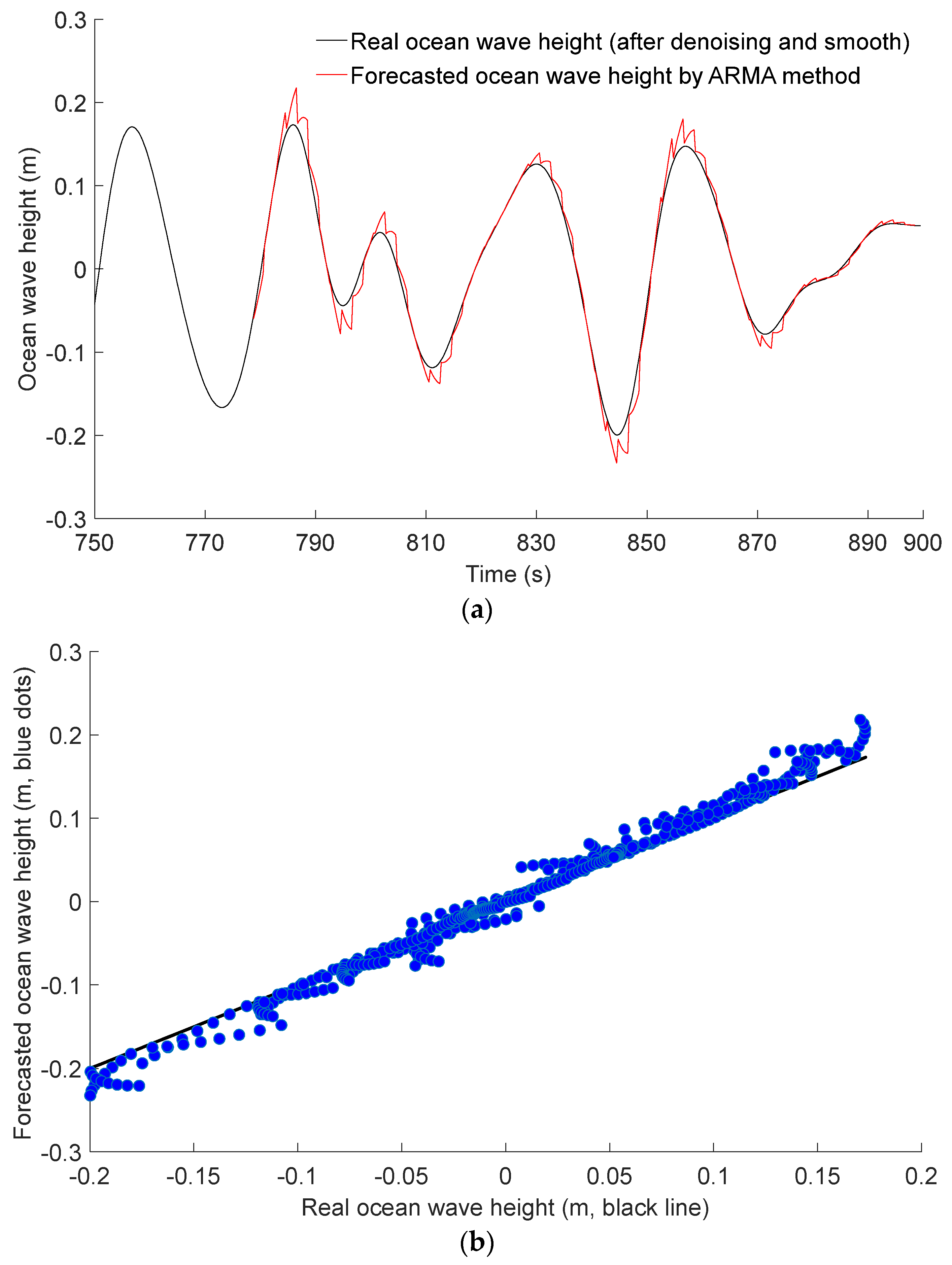
By the ARMA method,
Figure 7a shows the case of a 2-s lead forecast to the real ocean wave height, and the orders of the ARMA method are
and
. Compared with the real ocean wave height (after denoising and smoothing), forecast errors occur in the peak and trough areas of the ocean wave height.
Figure 7b shows the scatter plots depicting the forecasted ocean wave height versus the real ocean wave height.
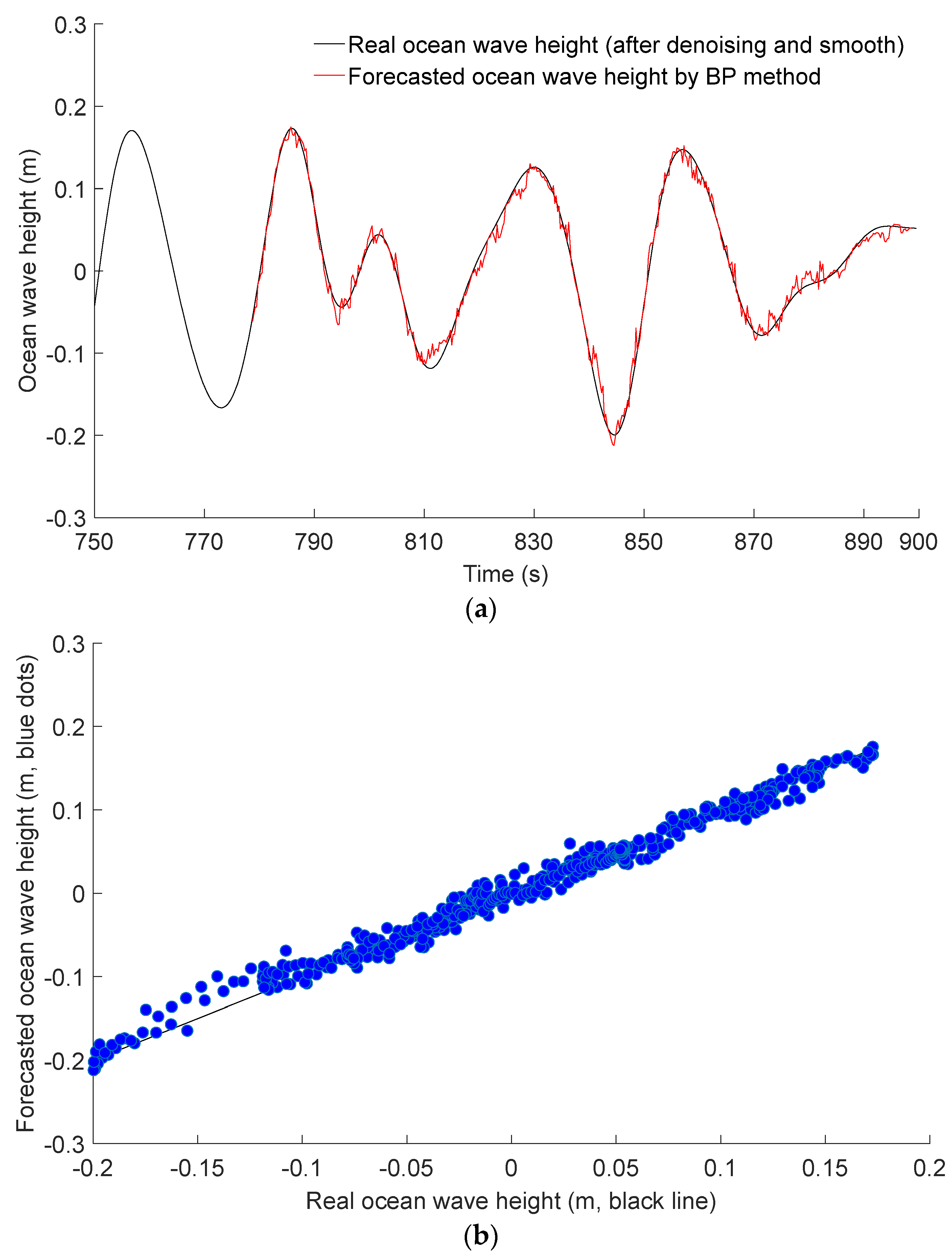
Under the same historical time series of real ocean wave height depicted in
Figure 7a,
Figure 8a presents the forecasted result of real ocean wave height using the BP neural network method, where the maximum training iterations were set at 500, with a training accuracy of 0.1 and a learning rate of 0.01. In
Figure 8a, the forecasted result is also 2 s ahead of the real ocean wave height. The historical time series of real ocean wave height consists of 116 data points, which are decomposed into a matrix of size (16 × 100) and a matrix of size (8 × 100) using the BP neural network method. By analyzing the relationship between the (16 × 100) matrix and the (8 × 100) matrix, future data are forecasted. Compared with the ARMA method of
Figure 7a, it can be seen that the forecasted result of the BP neural network method is superior, but some fluctuating errors always exist.
Figure 8b shows the scatter plots of forecasted ocean wave height against real ocean wave height.
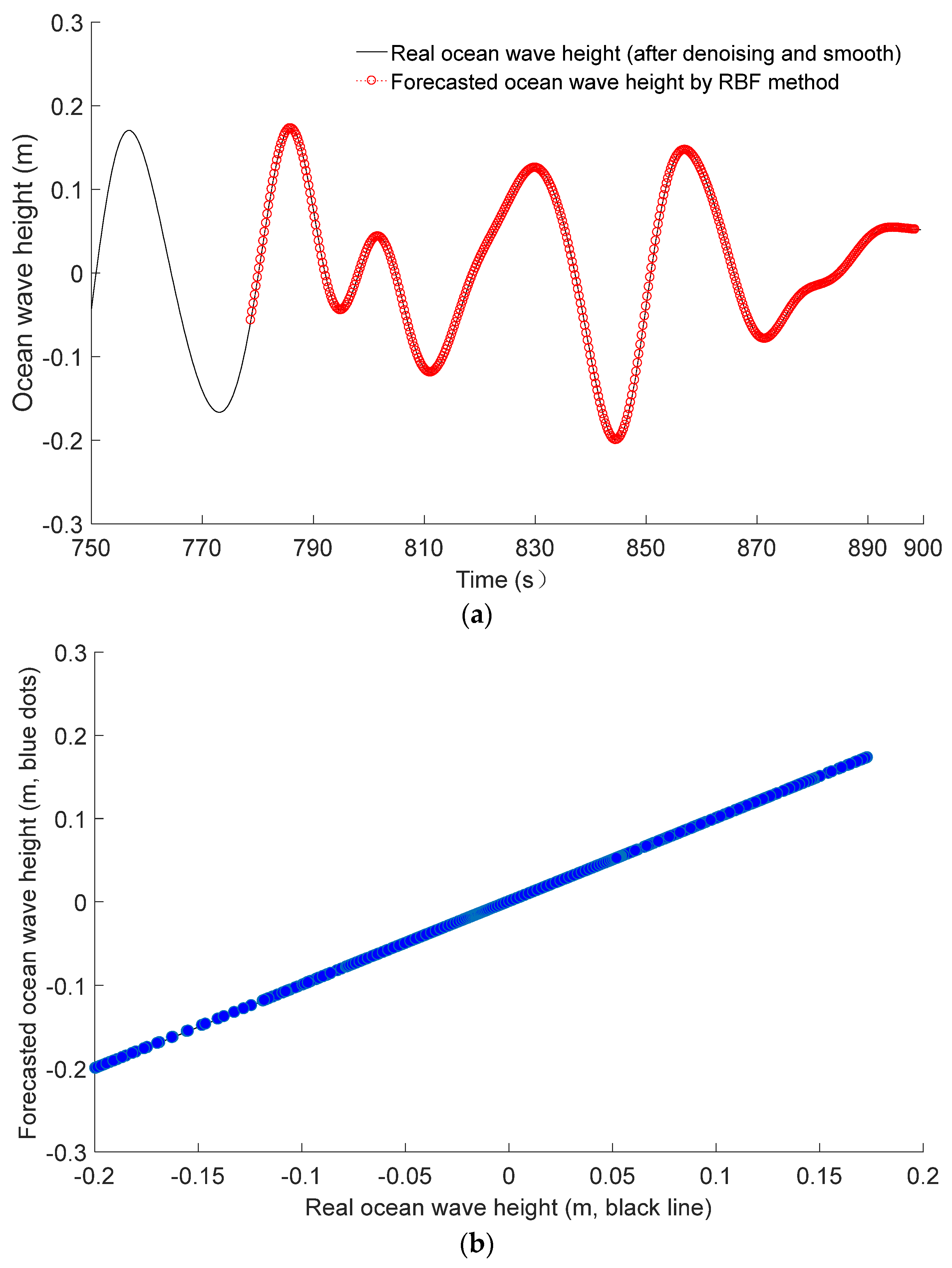
Figure 9a pertains to the 2-s-ahead forecast of future ocean wave height by the RBF neural network method, and
Figure 9b shows the scatter plots of forecasted ocean wave height against real ocean wave height. In
Figure 9a, the decomposition method for the historical time series of real ocean wave height is the same as that of the BP neural network method, but their training and forecasting methods differ (the fruit fly population is three, and the maximum number of iterations is two). The comparison among
Figure 7,
Figure 8 and
Figure 9 indicates that the forecast accuracy of the RBF neural network method is better than that of the other two methods.
In order to analyze and compare the forecast accuracy in detail,
Table 1 shows the quantitative performance of these three forecasting methods using RMSE, MAE and correlation coefficient R. From
Table 1, it can be seen that the RMSE and MAE of the RBF neural network are lower than those of the other methods, and the correlation coefficient R of the RBF neural network is the largest. Therefore, the comparison results of RMSE, MAE and the correlation coefficient R signify that the RBF neural network method is preferred over the other two methods.
In addition, even when the forecast time is extended, such as the 3-s-ahead forecast of real ocean wave height, the forecast accuracy of the RBF neural network method still exhibits the highest forecast accuracy, as shown in
Table 2.
Furthermore, compared with the calculation time consumption of the ARMA method and the BP neural network method, although the RBF neural network method has the longest calculation time consumption (
Table 1 and
Table 2), it is deemed acceptable due to the forecast time being 2 s or 3 s. In the practical application, 2 s or 3 s is sufficient for program execution and control signal output of the controller, particularly for controllers with high computational capabilities.
5. Discussions
In
Section 4, the comparison between
Table 1 and
Table 2 also shows that as the forecast time increases form 2 s to 3 s, the forecast errors (RMSE and MAE) of these three forecasting methods increase slightly, and the correlation coefficients
R of the BP neural network method and the RBF neural network method undergo a marginal decrease. This section discusses the reason for forecast errors and a general overview of the characteristics of these three forecasting methods.
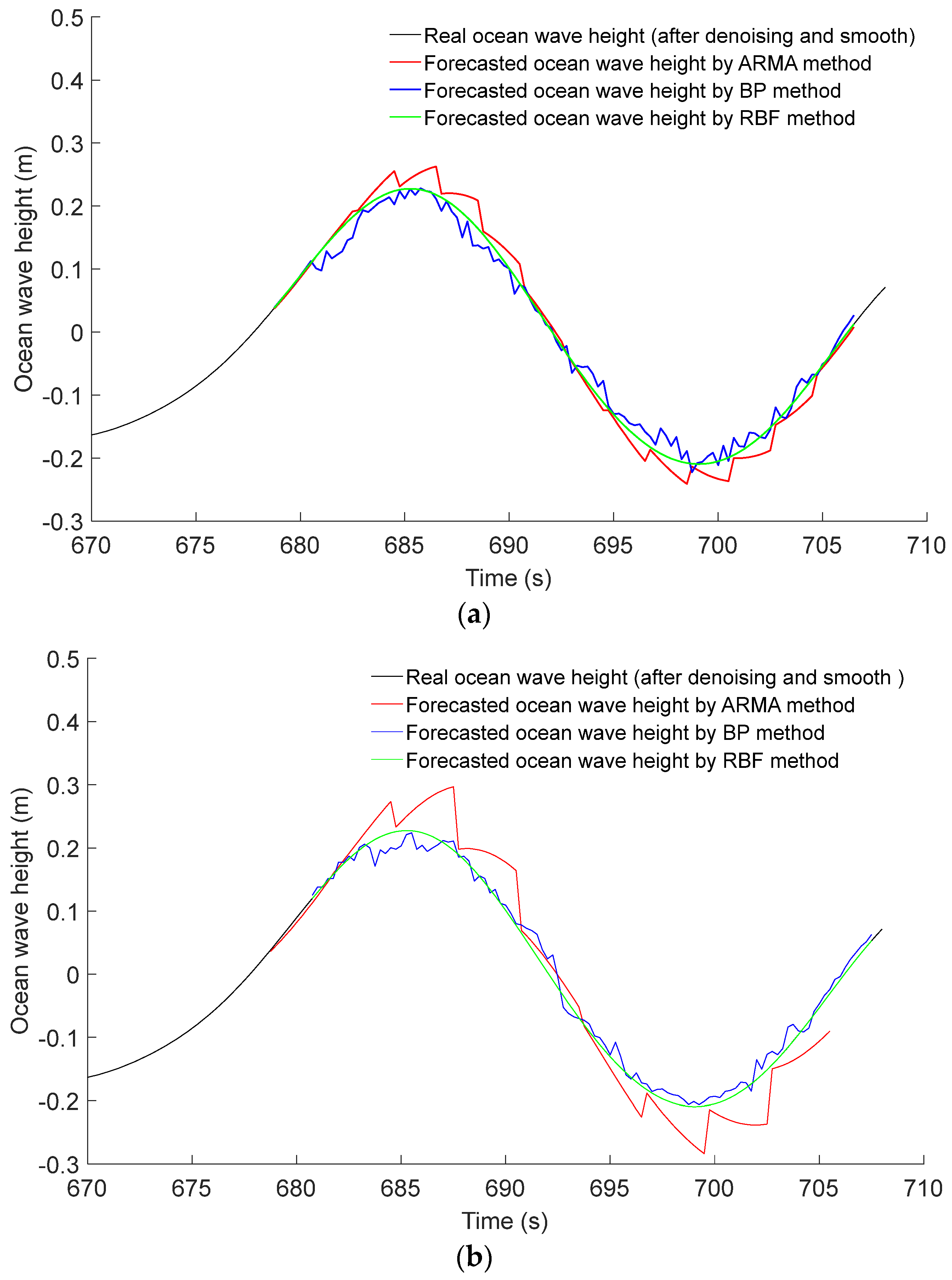
Through the method of curve plotting,
Figure 10 presents the forecast error comparison between the ARMA method, the BP neural network method and the RBF neural network method. From
Figure 10a,b, it can be concluded that the forecast errors of the ARMA method and the BP method exhibit greater magnitudes in the regions of peaks and troughs compared to other areas. This phenomenon arises due to the complete dependence of forecast values on the linear sequence Equation (2) and forward propagation Equation (4). For instance, in regions characterized by high rates of change in real ocean wave height, such as peaks and troughs, where the autoregressive coefficient and moving average coefficient do not change simultaneously, the forecast error of the ARMA method escalates. Conversely, leveraging the fruit fly optimization algorithm (FOA), the RBF neural network method demonstrates the advantage of minimal forecast error.
Figure 10a,b also show that the forecasted values of the BP neural network method exhibit fluctuations around the curve representing real ocean wave height. This behavior can be attributed to the real-time adjustment characteristic of the threshold value of in the hidden layer and the output layer. However, considering both the calculation time and number of iterative trainings, the forecast error of the BP neural network method is larger than the forecast error of the RBF neural network method.
By integrating the fruit fly optimization algorithm (FOA), the RBF neural network method successfully predicts future ocean wave heights, which closely align with the real ocean wave height, as depicted in
Figure 10a,b.
Therefore, the comparative analysis and subsequent discussion affirm that the RBF neural network method stands as the optimal approach for forecasting future ocean wave heights. Moreover, it has the potential to offer valuable data for the operation control and efficiency enhancement of ocean wave energy conversion systems. In practical applications, a forecast time (2~3 s) for ocean wave height suffices for program execution and signal processing of the current level controller. This optimization of the operational status of ocean wave energy conversion systems can lead to enhanced operational efficiency.
In addition, ocean wave field prediction holds significant importance for ensuring the operational safety of ocean wave energy conversion systems [
35,
36]. If future wave field prediction can provide information on ocean waves with larger wave heights (e.g., six-hours ahead of the real ocean wave height), proactive measures can be implemented to protect the ocean wave energy conversion system.
6. Conclusions
This paper adopts the Butterworth filter to denoise and smooth the curves of real ocean wave height. Subsequently, the ARMA method, the BP neural network method, and the RBF neural network method are utilized to forecast the ocean wave height. Upon comparing the forecast results of these three methods, it is evident that the RBF neural network method outperforms the other two forecasting methods. In addition, the computational time required by each forecasting method is compared, and the factors contributing to the forecast errors are analyzed.
The error comparison results of these three forecasting methods (
Figure 10a,b) indicate that a smoother curve corresponds to a higher forecast accuracy of future ocean wave height. Therefore, ocean waves with longer cycles (indicating smoother wave curves) can enhance the forecast accuracy of ocean wave height. In addition, in the practical design and implementation of ocean wave energy conversion systems, it is necessary to test and validate the feasibility of the RBF neural network forecasting method. Moreover, the installation position and seawater corrosion resistance of hardware components (e.g., controller and sensor, among others) should be taken into consideration.


