
Effect of Rigid Aquatic Bank Weeds on Flow Velocities and Bed Morphology


Abstract
1. Introduction
2. Methods and Materials
2.1. Dimensional Analysis
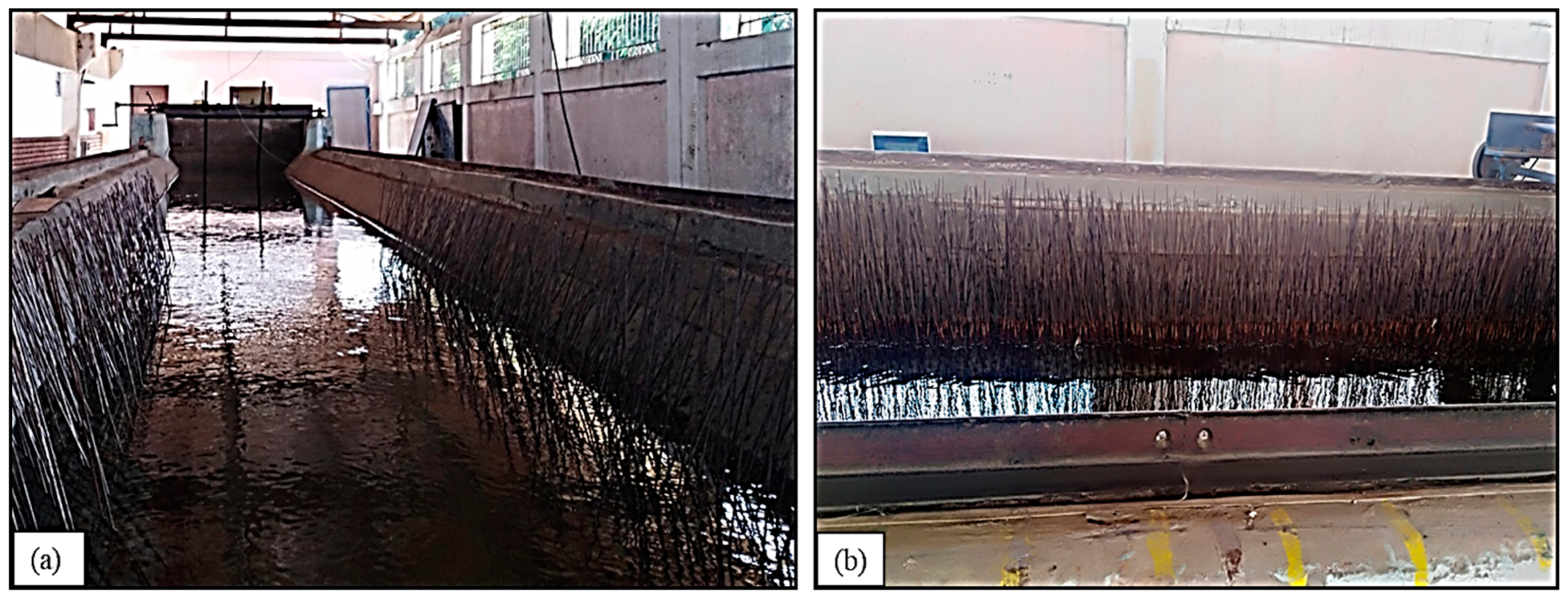
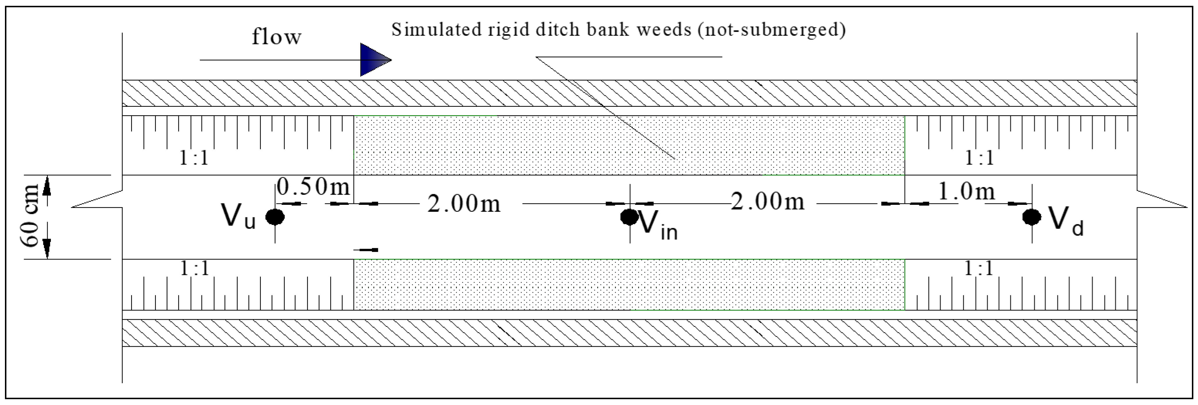
2.2. Experimental Setup
- The sand basin was filled with the tested sand and leveled to the channel bed level.
- The vegetation density and tail-water depth were adjusted according to the study run.
- The flume was filled to the required level by making the pumps circulate the flow very slowly until the flow was adjusted to the required value (25, 30, 35, and 40 L/s) using the control valve.
- The experiment was run for the equilibrium time, which was estimated later, and then the feeding pump was turned off.
- Water was drained out slowly until the formed sand holes became visible.
- Bed scour holes were surveyed every 0.16 and 0.12 m in the longitudinal and transverse directions, respectively.
3. Results and Discussion
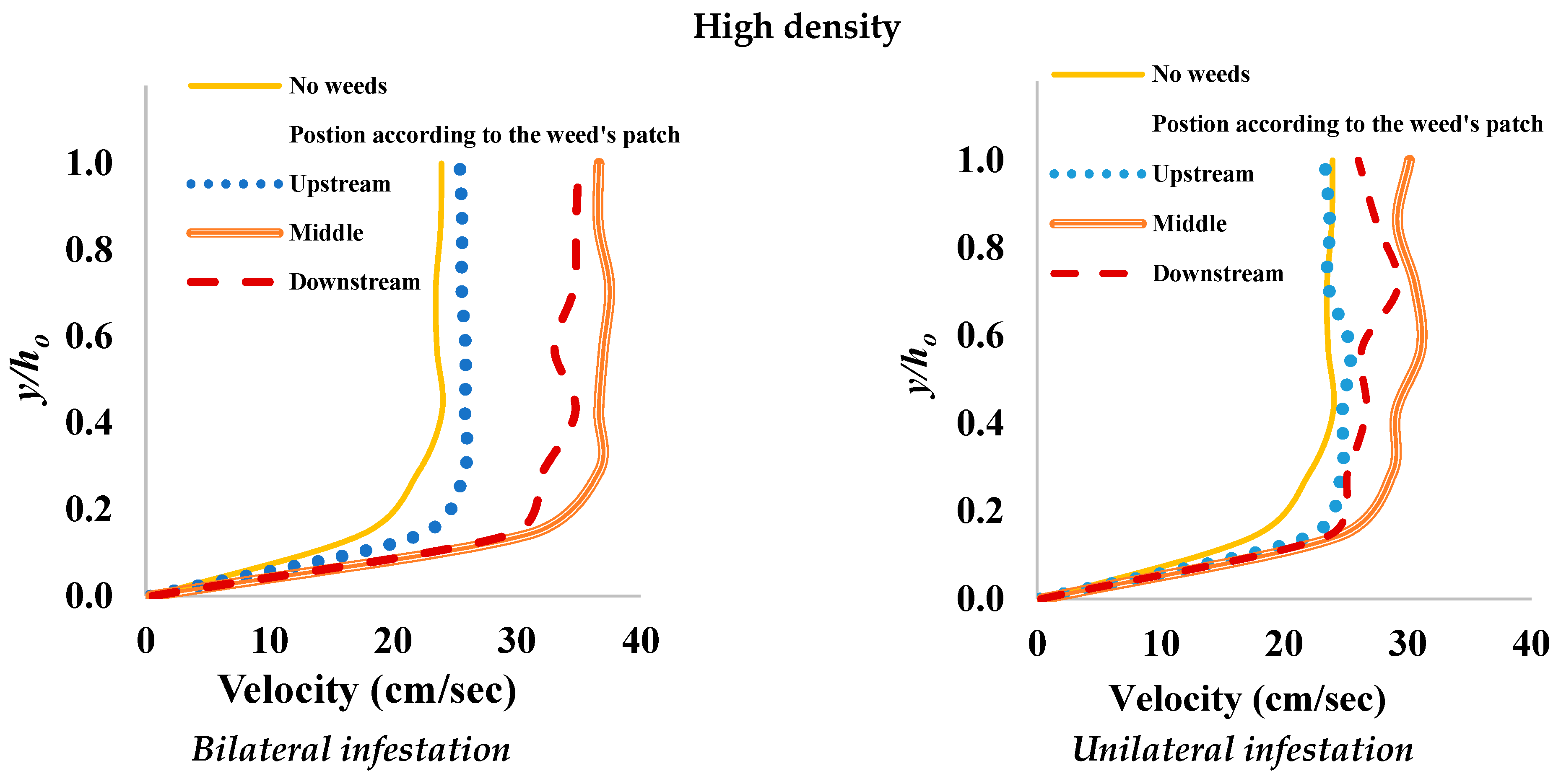
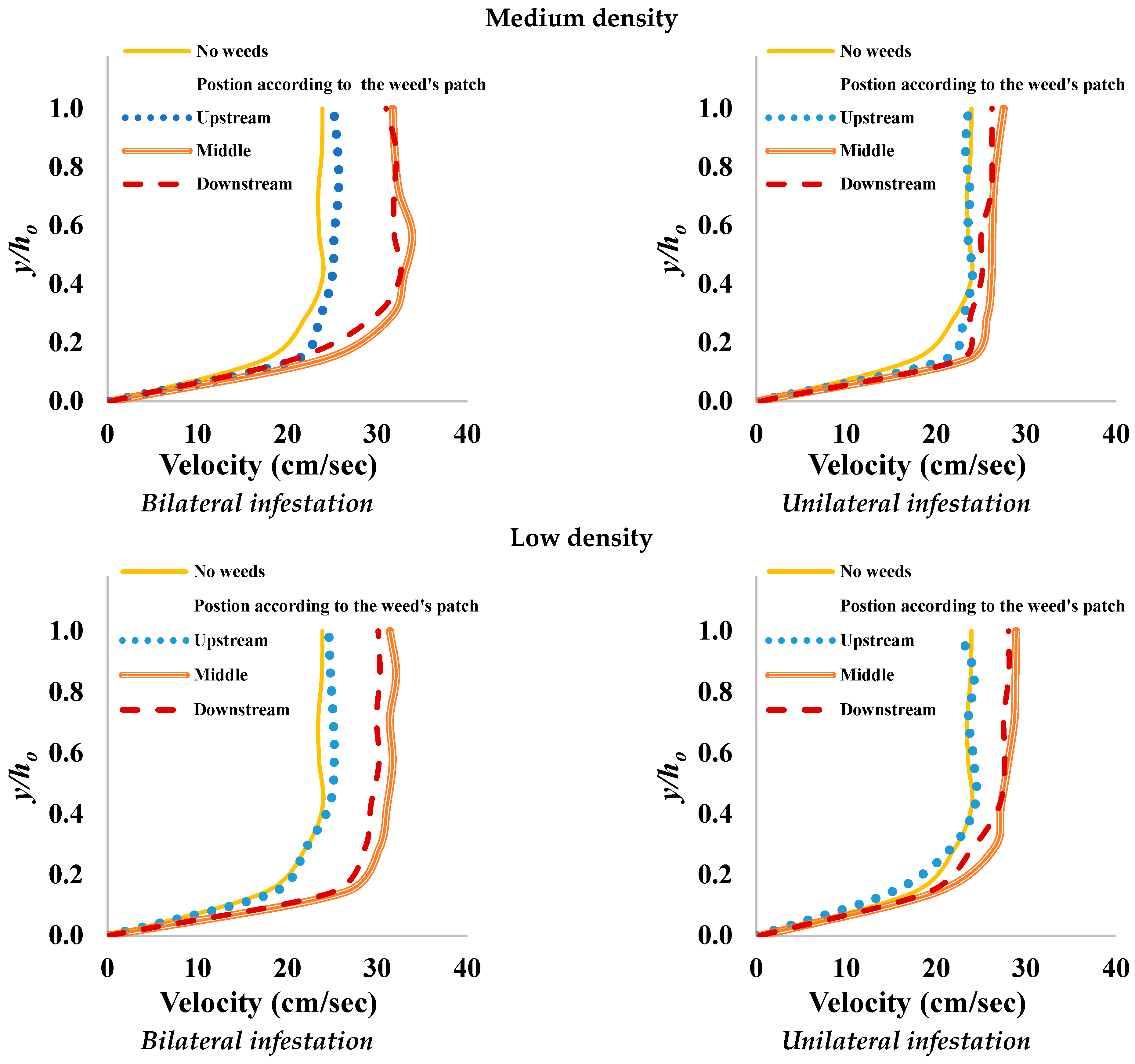
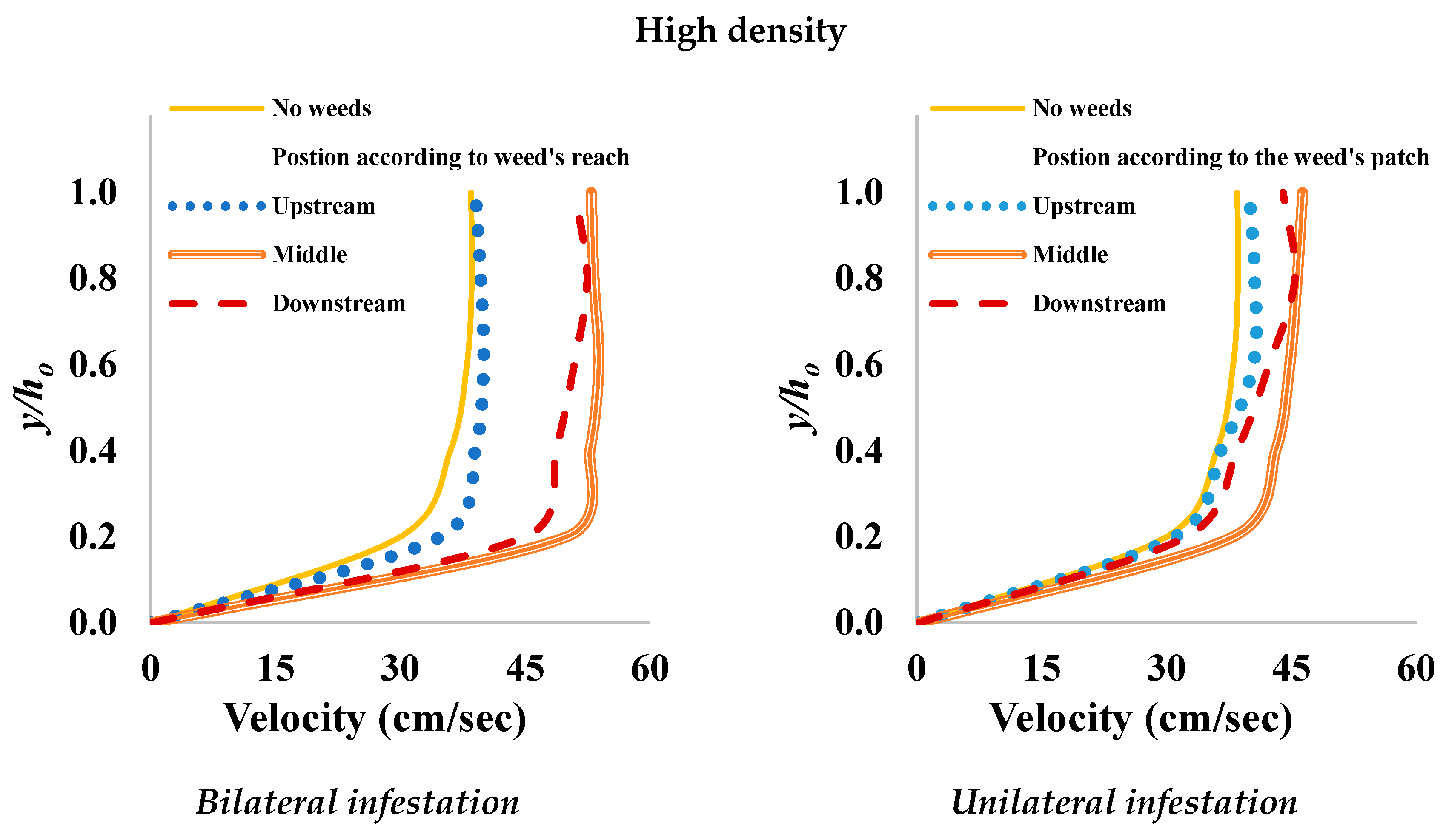
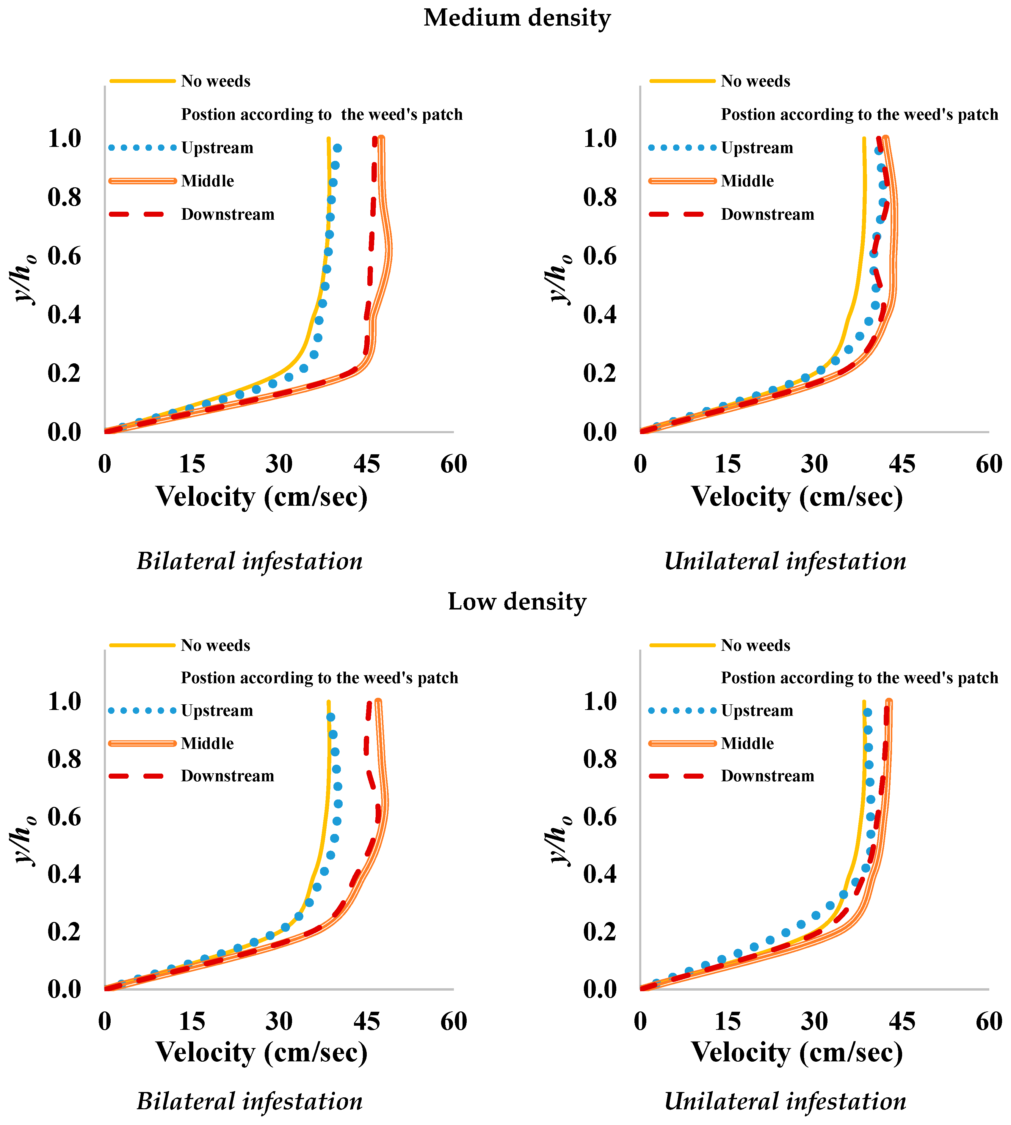
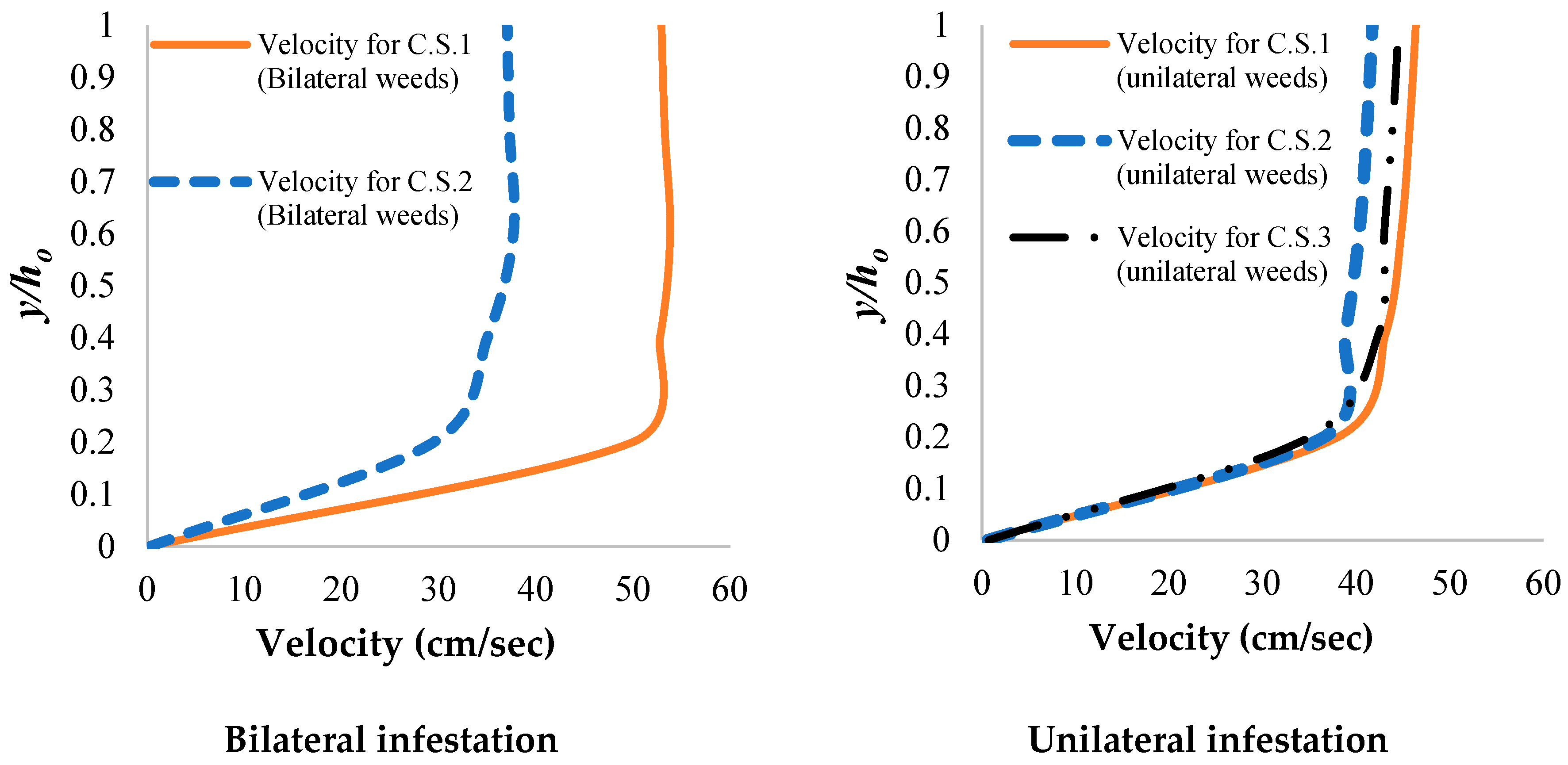
3.1. Vertical Velocity Profile
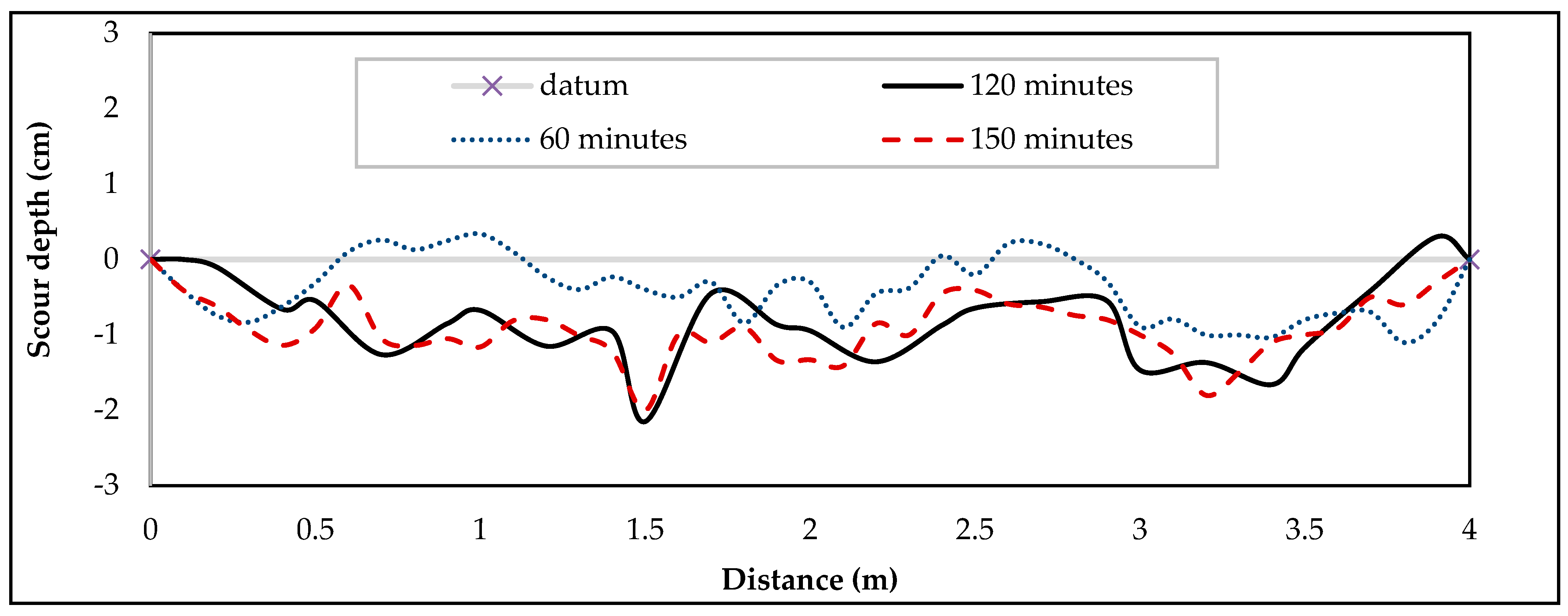
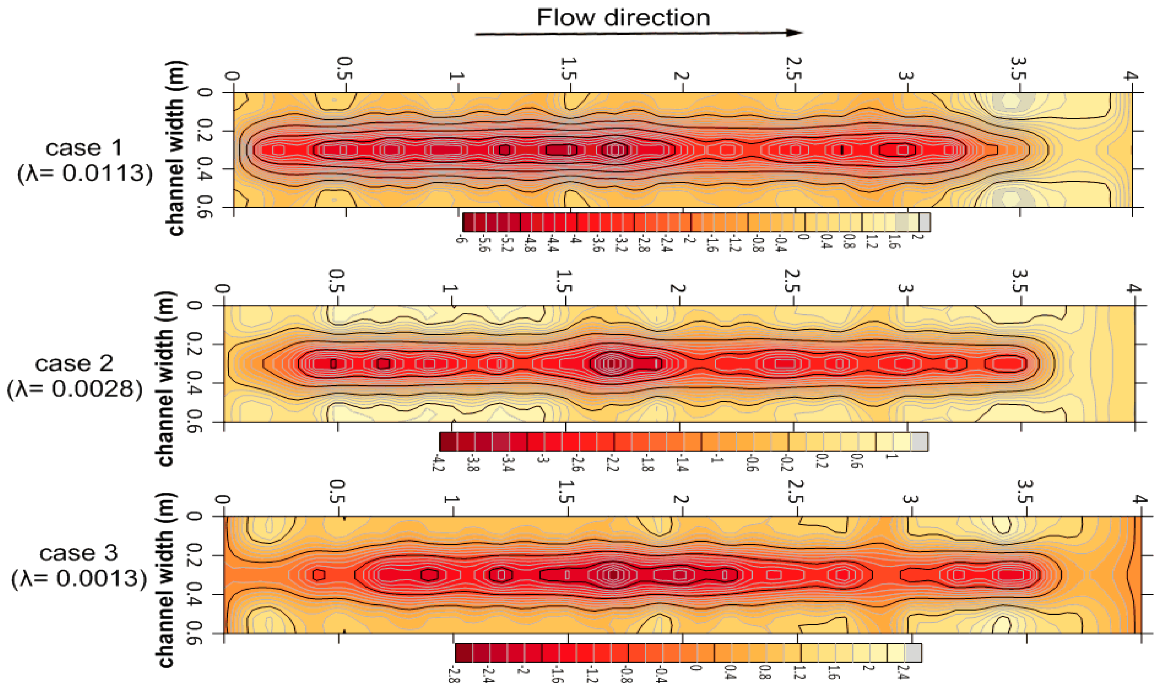
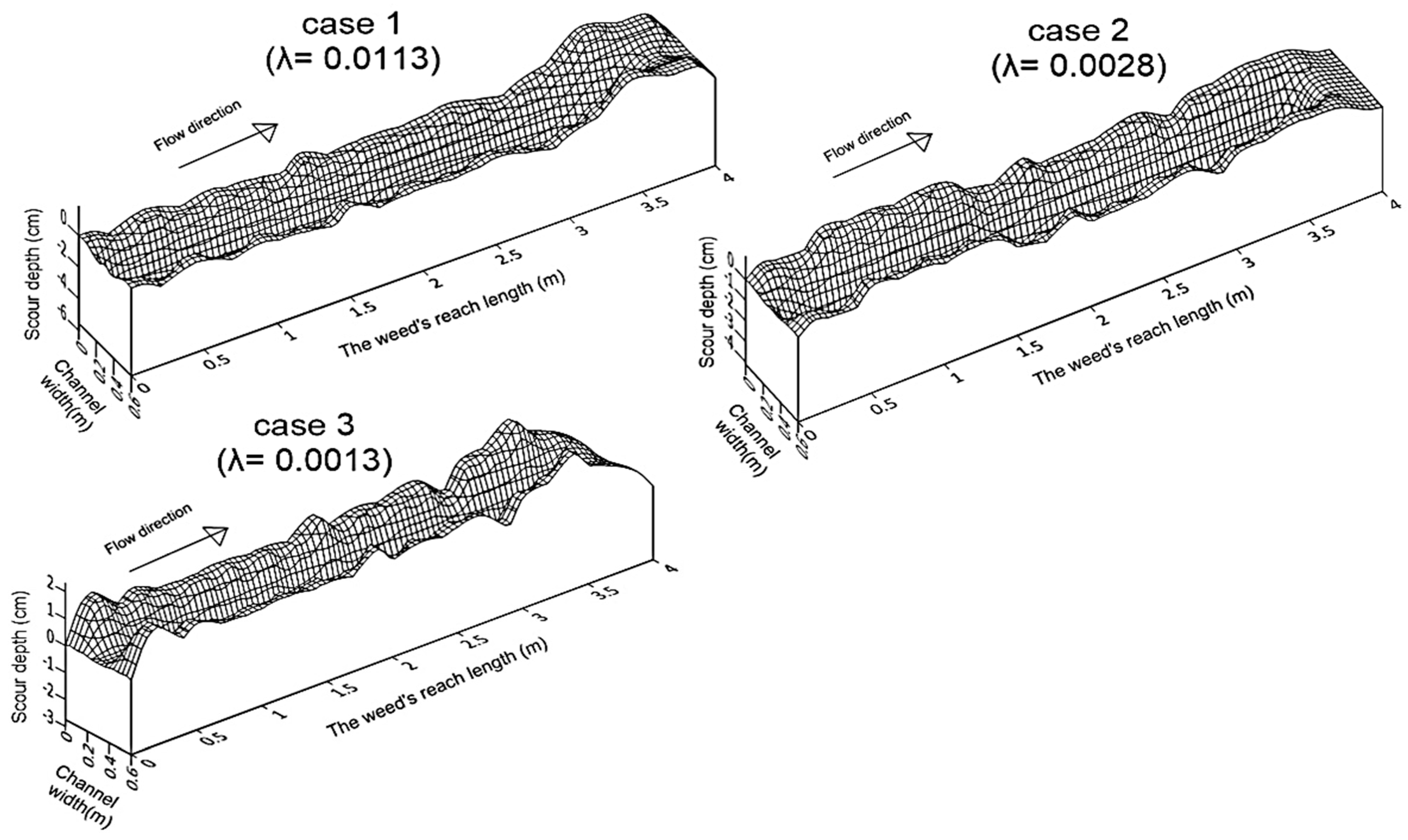
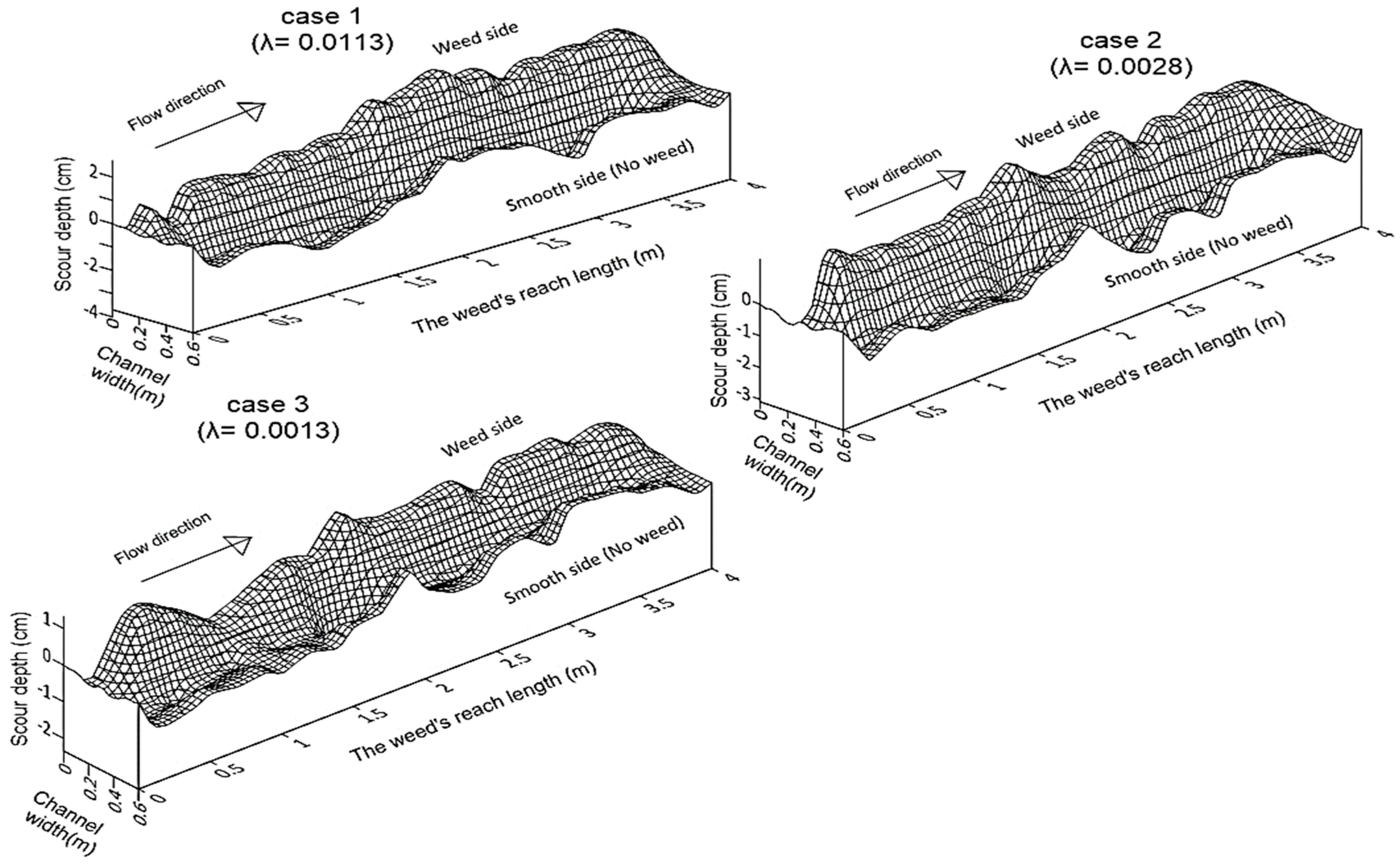
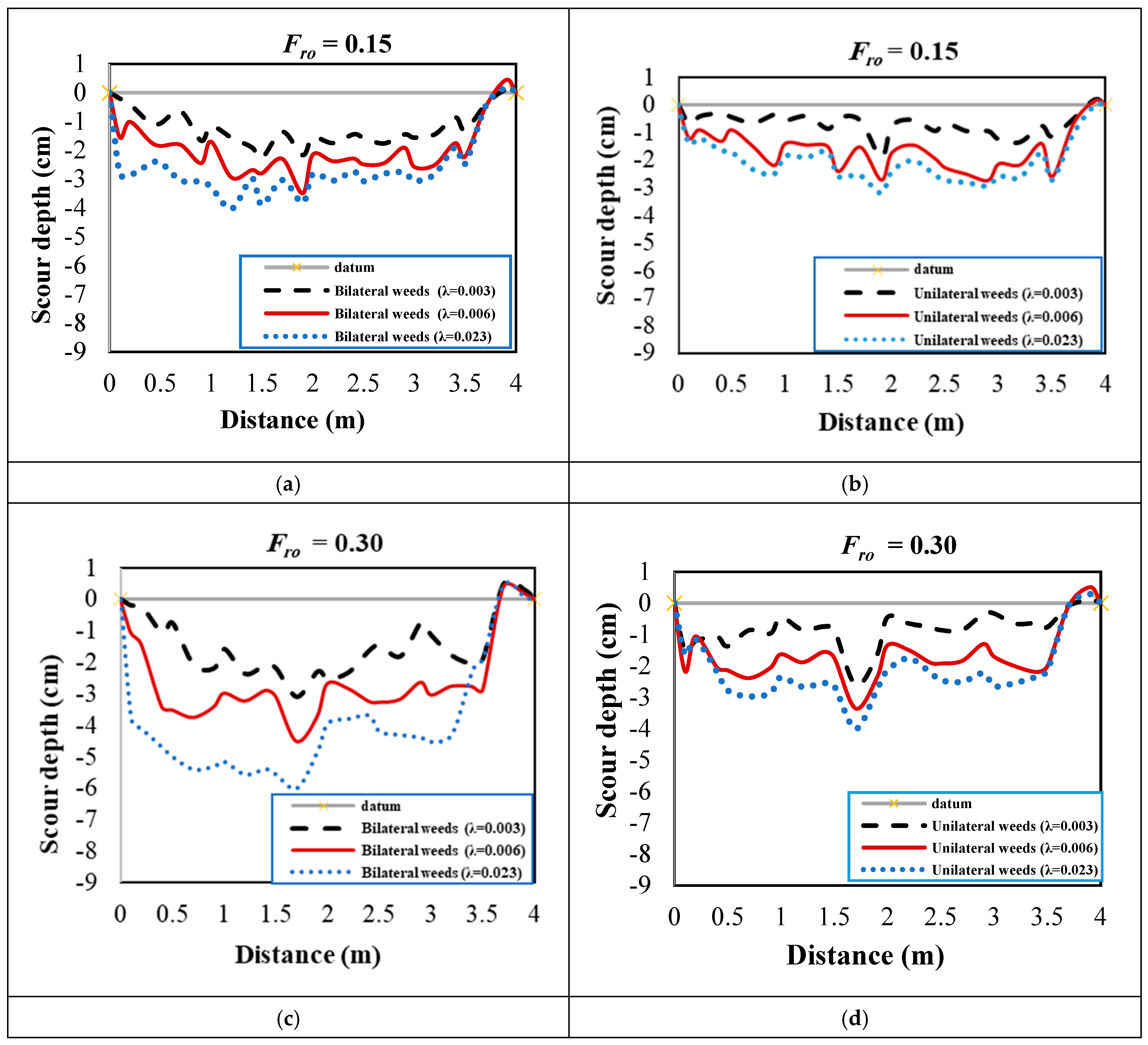
3.2. Bed Morphology
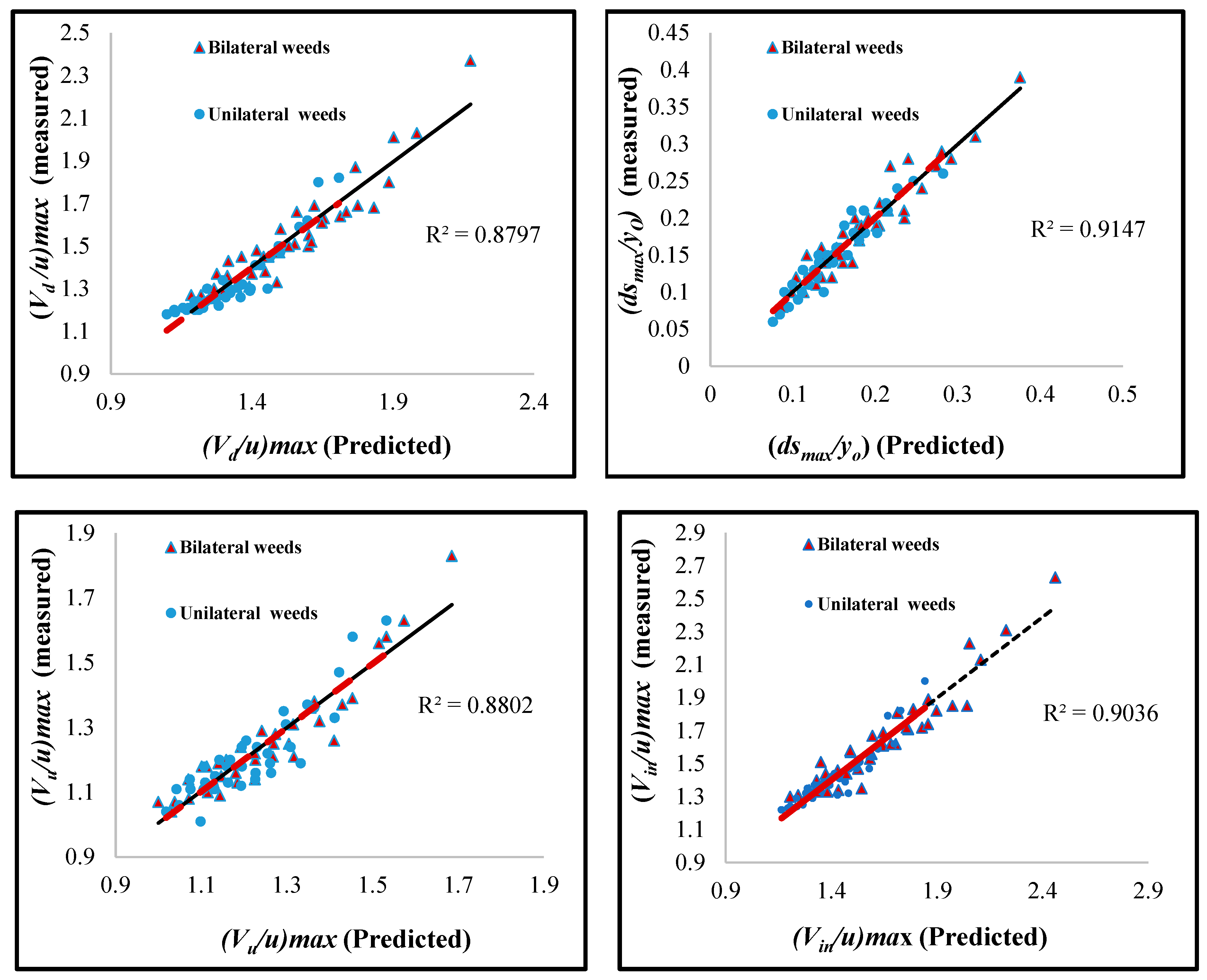
3.3. Relative Velocity and Maximum Scour Depth Estimation
3.4. Research Application
4. Conclusions
Author Contributions
Funding
Data Availability Statement
Acknowledgments
Conflicts of Interest
References
- Galema, A.A. Vegetation Resistance Evaluation of Vegetation Resistance Descriptors for Flood Management. Master’s Thesis, University of Twente, Enschede, The Netherlands, 2009. [Google Scholar]
- El Samman, T.A.; El Ella, S.M.A. Aquatic weeds monitoring and associated problems in Egyptian Channels. In Proceedings of the Thirteenth International Water Technology Conference, Hurghada, Egypt, 12–15 March 2009. [Google Scholar]
- Kemp, J.L.; Harper, D.M.; Crosa, G.A. The habitat-scale eco-hydraulics of rivers. J. Ecol. Eng. JEE 2000, 16, 17–29. [Google Scholar] [CrossRef]
- Tang, H.; Lu, S.; Zhou, Y.; Xu, X.; Xiao, Y. Water environment improvements in Zhenjiang City, China. ICE-Munic. Eng. 2008, 161, 11–16. [Google Scholar] [CrossRef]
- Nepf, H.M. Hydrodynamics of Vegetated Channels. J. Hydraul. Resour. 2012, 50, 262–279. [Google Scholar] [CrossRef]
- Kim, H.S.; Nabi, M.; Kimura, I. Computational modeling of flow and morphodynamics through rigid-emergent vegetation. Adv. Water Resour. 2015, 84, 64–86. [Google Scholar] [CrossRef]
- Xu, Z.X.; Ye, C.; Zhang, Y. 2D Numerical Analysis of the Influence of Near-Bank Vegetation Patches on the Bed Morphological Adjustment. In Environmental Fluid Mechanics; Springer: Berlin/Heidelberg, Germany, 2020. [Google Scholar] [CrossRef]
- Hopkinson, L.C.; Wynn-Thompson, T.M. Comparison of direct and indirect boundary shear stress measurements along vegetated streambanks. River Res. Appl. 2016, 32, 1755–1764. [Google Scholar] [CrossRef]
- Afzalimehr, H.; Dey, S. Influence of bank vegetation and gravel bed on velocity and Reynolds stress distributions. Int. J. Sediment Res. 2009, 24, 236–246. [Google Scholar] [CrossRef]
- Hirschowitz, P.M.; James, C.S. Conveyance estimation in channels with emergent bank vegetation. Water SA 2009, 35, 607–614. [Google Scholar] [CrossRef][Green Version]
- Afzalimehr, H.; Fazel, N.E.; Singh, V.P. Effect of Vegetation on Banks on Distributions of Velocity and Reynolds Stress under Accelerating Flow. J. Hydrol. Eng. ASCE 2010, 15, 708–713. [Google Scholar] [CrossRef]
- Mohammadzade, N.; Afzalimehr, H.; Singh, V.P. Experimental Investigation of Influence of Vegetation on Flow Turbulence. Int. J. Hydraul. Eng. 2016, 4, 54–69. [Google Scholar] [CrossRef]
- Liu, D.; Valyrakis, M.; Williams, R. Flow Hydrodynamics across Open Channel Flows with Riparian Zones: Implications for Riverbank Stability. Water 2017, 9, 720. [Google Scholar] [CrossRef]
- Valyrakis, M.; Liu, D.; Turker, U. The role of increasing riverbank vegetation density on flow dynamics across an asymmetrical channel. Environ. Fluid Mech. 2021, 21, 643–666. [Google Scholar] [CrossRef]
- Eraky, O.M.; Eltoukhy, M.A.; Abdelmoaty, M.S. Effect of rigid, bank vegetation on velocity distribution and water surface profile in open channel. Water Pract. Technol. 2022, 17, 1445–1457. [Google Scholar] [CrossRef]
- James, C.S.; Birkhead, A.L.; Jordanova, A.A.; O’Sullivan, J.J. Flow resistance of emergent vegetation. J. Hydraul. Res. 2004, 42, 390–398. [Google Scholar] [CrossRef]
- Huai, W.X.; Chen, Z.B.; Jie, H.A.N.; Zhang, L.X.; Zeng, Y.H. Mathematical model for the flow with submerged and emerged rigid vegetation. J. Hydrodyn. Ser. B 2009, 21, 722–729. [Google Scholar] [CrossRef]
- Liu, C.; Shan, Y. Impact of an emergent model vegetation patch on flow adjustment and velocity. Proc. Inst. Civ. Eng. Water Manag. 2022, 175, 55–66. [Google Scholar] [CrossRef]
- Van de Lageweg, W.I.; van Dijk, W.M.; Hoendervoogt, R. Effects of riparian vegetation on experimental channel dynamics. In International Conference on Fluvial Hydraulics: River Flow; Bundesanstalt für Wasserbau Braunschweig: Karlsruhe, Germany, 2010. [Google Scholar]
- Yang, S.; Bai, Y.; Xu, H. Experimental analysis of river evolution with riparian vegetation. Water 2018, 10, 1500. [Google Scholar] [CrossRef]
- Abdelhaleem, F.S.; Mohamed, I.M.; Shaaban, I.G.; Ardakanian, A.; Fahmy, W.; Ibrahim, A. Pressure-Flow Scour under a Bridge Deck in Clear Water Conditions. Water 2023, 15, 404. [Google Scholar] [CrossRef]
- Li, J.F.; Tfwala, S.S.; Chen, S.C. Effects of vegetation density and arrangement on sediment budget in a sediment-laden flow. Water 2018, 10, 1412. [Google Scholar] [CrossRef]
- Vargas-Luna, A.; Crosato, A.; Calvani, G. Representing plants as rigid cylinders in experiments and models. Adv. Water Resour. 2016, 93, 205–222. [Google Scholar] [CrossRef]
- Vargas-Luna, A.; Duró, G.; Crosato, A. Morphological Adaptation of River Channels to Vegetation Establishment: A Laboratory Study. J. Geophys. Res. Earth Surf. 2019, 124, 1981–1995. [Google Scholar] [CrossRef]
- Azarisamani, A.; Keshavarzi, A.; Hamidifar, H.; Javan, M. Effect of rigid vegetation on velocity distribution and bed topography in a meandering river with a sloping bank. Arab. J. Sci. Eng. 2020, 45, 8633–8653. [Google Scholar] [CrossRef]
- Schoneboom, T.; Aberle, J.; Dittrich, A. Spatial variability, mean drag forces, and drag coefficients in an array of rigid cylinders. In Experimental Methods in Hydraulic Research; Rowinski, P., Ed.; Springer: Berlin/Heidelberg, Germany, 2011; Volume 1, pp. 255–265. [Google Scholar]
- Jumain, M.; Ibrahim, Z.; Ismail, Z. Hydraulic and morphological patterns in a riparian vegetated sandy compound straight channel. IOP Conf. Ser. Earth Environ. Sci. 2021, 646, 012036. [Google Scholar] [CrossRef]
- Stone, B.M.; Shen, H.T. Hydraulic resistance of flow in channels with cylindrical roughness. J. Hydraul. Eng. 2002, 128, 500–506. [Google Scholar] [CrossRef]
- Meftah, M.B.; De Serio, F.; Malcangio, D.; Perrillo, A.F.; Mossa, M. Experimental study of flexible and rigid vegetation in an open channel. In Proceedings of the River Flow Conference on Fluvial Hydraulics, River Flow, Lisbon, Portugal, 6–8 September 2006; Volume 1, pp. 603–611. [Google Scholar]
- Kothyari, U.C.; Hayashi, K.; Hashimoto, H. Drag coefficient of unsubmerged rigid vegetation stems in open-channel flows. J. Hydraul. Res. 2009, 47, 691–699. [Google Scholar] [CrossRef]
- Cheng, N.S.; Nguyen, H.T. Hydraulic radius for evaluating resistance induced by simulated emergent vegetation in open-channel flows. J. Hydraul. Eng. 2011, 137, 995–1004. [Google Scholar] [CrossRef]
- Panigrahi, K. Experimental Study of Flow-Through Rigid Vegetation in Open Channel. Master’s Thesis, National Institute of Technology, Rourkela, Odisha, India, 2015. [Google Scholar]
- Ahmed, M.; Hady, A. Evaluation of emergent vegetation resistance and comparative study between last descriptors. Control Sci. Eng. 2017, 1, 1–7. [Google Scholar]
- Chakraborty, P.; Sarkar, A. Study of flow characteristics within randomly distributed submerged rigid vegetation. J. Hydrodyn. 2018, 31, 358–367. [Google Scholar] [CrossRef]
- Tong, X.; Liu, X.; Yang, T.; Hua, Z.; Wang, Z.; Liu, J.; Li, R. Hydraulic features of flow through local non-submerged rigid vegetation in the Y-shaped confluence channel. Water 2019, 11, 146. [Google Scholar] [CrossRef]
- D’Ippolito, A.; Calomino, F.; Penna, N.; Dey, S.; Gaudio, R. Simulation of Accelerated Subcritical Flow Profiles in an Open Channel with Emergent Rigid Vegetation. Appl. Sci. 2022, 12, 6960. [Google Scholar] [CrossRef]
- Lee, J.; Jeong, Y.M.; Kim, J.S.; Hur, D.S. Analysis of hydraulic characteristics according to the cross-section changes in submerged rigid vegetation. J. Ocean Eng. Technol. 2022, 36, 326–339. [Google Scholar] [CrossRef]
- Wang, Q.; Zhang, Y.; Wang, P.; Feng, T.; Bai, Y. Longitudinal velocity profile of flows in open channel with double-layered rigid vegetation. Front. Environ. Sci. 2023, 10, 1094572. [Google Scholar] [CrossRef]
- Huang, T.; He, M.; Hong, K.; Lin, Y.; Jiao, P. Effect of Rigid Vegetation Arrangement on the Mixed Layer of Curved Channel Flow. J. Mar. Sci. Eng. 2023, 11, 213. [Google Scholar] [CrossRef]
- Li, J.; Claude, N.; Tassi, P.; Cordier, F.; Vargas-Luna, A.; Crosato, A.; Rodrigues, S. Effects of vegetation patch patterns on channel morphology: A numerical study. J. Geophys. Res. Earth Surf. 2022, 127, e2021JF006529. [Google Scholar] [CrossRef]
- Lin, Y.-T.; Ye, Y.-Q.; Han, D.-R.; Chiu, Y.-J. Propagation and Separation of Down slope Gravity Currents over Rigid and Emergent Vegetation Patches in Linearly Stratified Environments. J. Mar. Sci. Eng. 2022, 10, 308. [Google Scholar] [CrossRef]
- Mofrad, M.R.T.; Afzalimehr, H.; Parvizi, P.; Ahmad, S. Comparison of Velocity and Reynolds Stress Distributions in a Straight Rectangular Channel with Submerged and Emergent Vegetation. Water 2023, 15, 2435. [Google Scholar] [CrossRef]
- Dey, S.; Raikar, R.V.; Roy, A. Scour at submerged cylindrical obstacles under steady flow. J. Hydraul. Eng. 2008, 134, 105–109. [Google Scholar] [CrossRef]
- Devi, T.B.; Kumar, B. Experimentation on submerged flow over flexible vegetation patches with downward seepage. Ecol. Eng. 2016, 91, 158–168. [Google Scholar] [CrossRef]
- Amir, M.U.; Hashmi, H.N.; Baloch, M. Experimental investigation of channel bank vegetation on scouring characteristics around a wing wall abutment. Tech. J. Univ. Eng. Technol. UET 2018, 23, 15–21. [Google Scholar]
- Eraky, O.M.; Eltoukhy, M.A.; Abdelmoaty, M.S. Heading Up and Head Losses Estimation Due to Rigid BankVegetation. Eng. Res. J. ERJ 2023, 52, 64–72. [Google Scholar] [CrossRef]


| Authors | Equation | Remark |
|---|---|---|
| James et al., 2004 [16] | F: resistance coefficient accounting for stem drag; S: channel slope; N: number of stems per unit area; d: stem diameter; Cd: drag coefficient. | |
| Hirschowitz and James 2009 [10] | A: cross-sectional area of the un-vegetated zone; B: bed width; h: flow depth at the interface; fb: friction factor of the bed; fv: friction factor of the vegetation interface. | |
| Huai et al., 2009 [17] | D: cylinder diameter. m: number of stems in the control volume = 1/(xa ya); i: energy slope. | |
| Valyrakis et al., 2021 [14] | φ: solid volume fraction (φ = mπD2/(4LWv); u: mean velocity in the no-weeds case. | |
| Liu and Shan 2022 [18] | S: water surface slope; Φ: solid volume fraction (=(π/4)nd2); Cf: bed friction coefficient; Cd: drag coefficient; a: frontal area per patch volume (=nd); h: flow depth. |
| Authors | Stem Simulation | ||||
|---|---|---|---|---|---|
| Shaped | Material | Diameter (mm) | Spacing (Δx) | Distribution | |
| James et al. [16] | Cylindrical | Steel | 5 | 2.5, 5, and 7.5 cm | Staggered |
| Stone and Shen [28] | Wood | 3.18, 6.35 and 12.7 | 3.8, 4.6 and 7.6 cm | Staggered | |
| Meftah et al. [29] | Steel | 3 | 10 cm | Linear | |
| Kothyari et al. [30] | Stainless steel | 10 | 3.2 to 20.3 cm | Staggered | |
| Cheng and Nguyen [31] | Steel | 3.2, 6.6 and 8.3 | 3 and 6 cm | Staggered | |
| Panigrahi [32] | Steel | 6.5 | 10 cm | Both linear and staggered | |
| Ahmed and Hady [33] | PVC | 10 | 22.72, 11.9, and 9.61 cm | Linear | |
| Chakraborty and Sarkar [34] | PVC | 6 | Random Distribution | ||
| Tong et al. [35] | PVC | 8 | 10 cm | Linear | |
| D’Ippolito et al. [36] | Wood | 8 and 10 | 4.24 and 8.48 cm | Both linear and staggered | |
| Lee et al. [37] | Acrylic | 10 | 4 and 8 cm | staggered | |
| Wang et al. [38] | PVC | 6 | 6 cm | Linear | |
| Huang et al. [39] | Wood | 6 | 2.5 and 5 cm | Linear | |
| Current study | Steel | 3 | 2.5, 5, and 7.5 cm | Staggered | |
| Weeds Configuration | Bed Condition | Discharge (L/s) | Tail Water Depth | No of Runs | ||
|---|---|---|---|---|---|---|
| Density/m | Arrangement | Spacing cm | ||||
| No weeds | n/a | n/a | concrete | 40,35,30,25 L/s | Three different tail depths for each discharge | 12 |
| High (λ~0.013) | Staggered both bilateral and unilateral weeds | 2.5 | 40,35,30,25 L/s | 24 | ||
| Medium (λ~0.0028) | 5.0 | 40,35,30,25 L/s | 24 | |||
| Low (λ~0.0013) | 7.5 | 40,35,30,25 L/s | 24 | |||
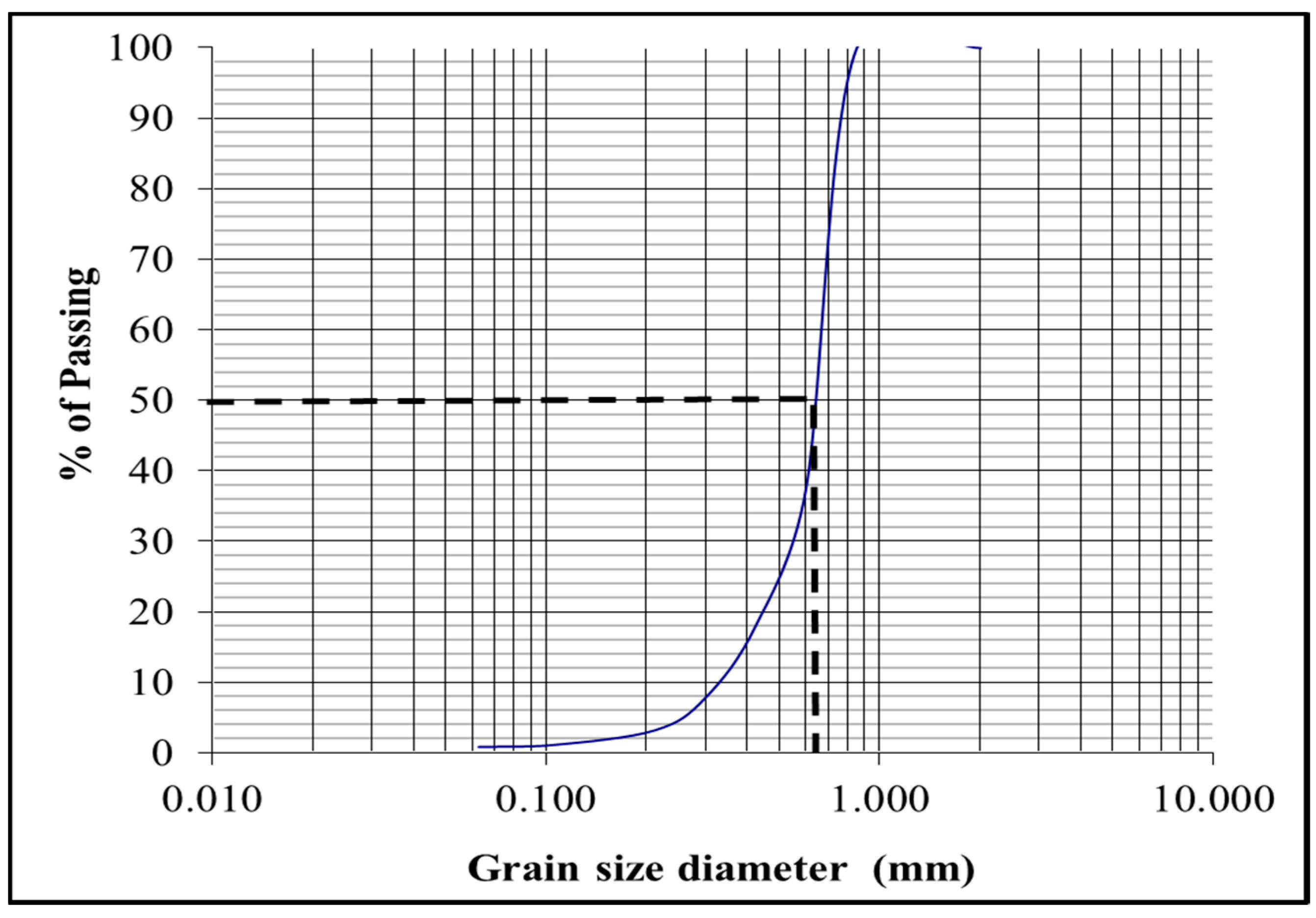
| No weeds | n/a | n/a | Sandy soil with D50 = 0.65 | 40,35,30,25 L/s | 12 | |
| High (λ~0.013) | Staggered both bilateral and unilateral weeds | 2.5 | 40,35,30,25 L/s | 24 | ||
| Medium (λ~0.0028) | 5.0 | 40,35,30,25 L/s | 24 | |||
| Low (λ~0.0013) | 7.5 | 40,35,30,25 L/s | 24 | |||
| Total Number of Runs | 168 | |||||
| Arrangement | Density | Velocity Position | ||
|---|---|---|---|---|
| Upstream | Middle | Downstream | ||
| Bilateral infestation | High | 9% | 50% | 43% |
| Medium | 4% | 32% | 28% | |
| Low | 2% | 27% | 24% | |
| Unilateral infestation | High | 4% | 24% | 17% |
| Medium | 2% | 12% | 9% | |
| Low | 1.4% | 12% | 8% | |
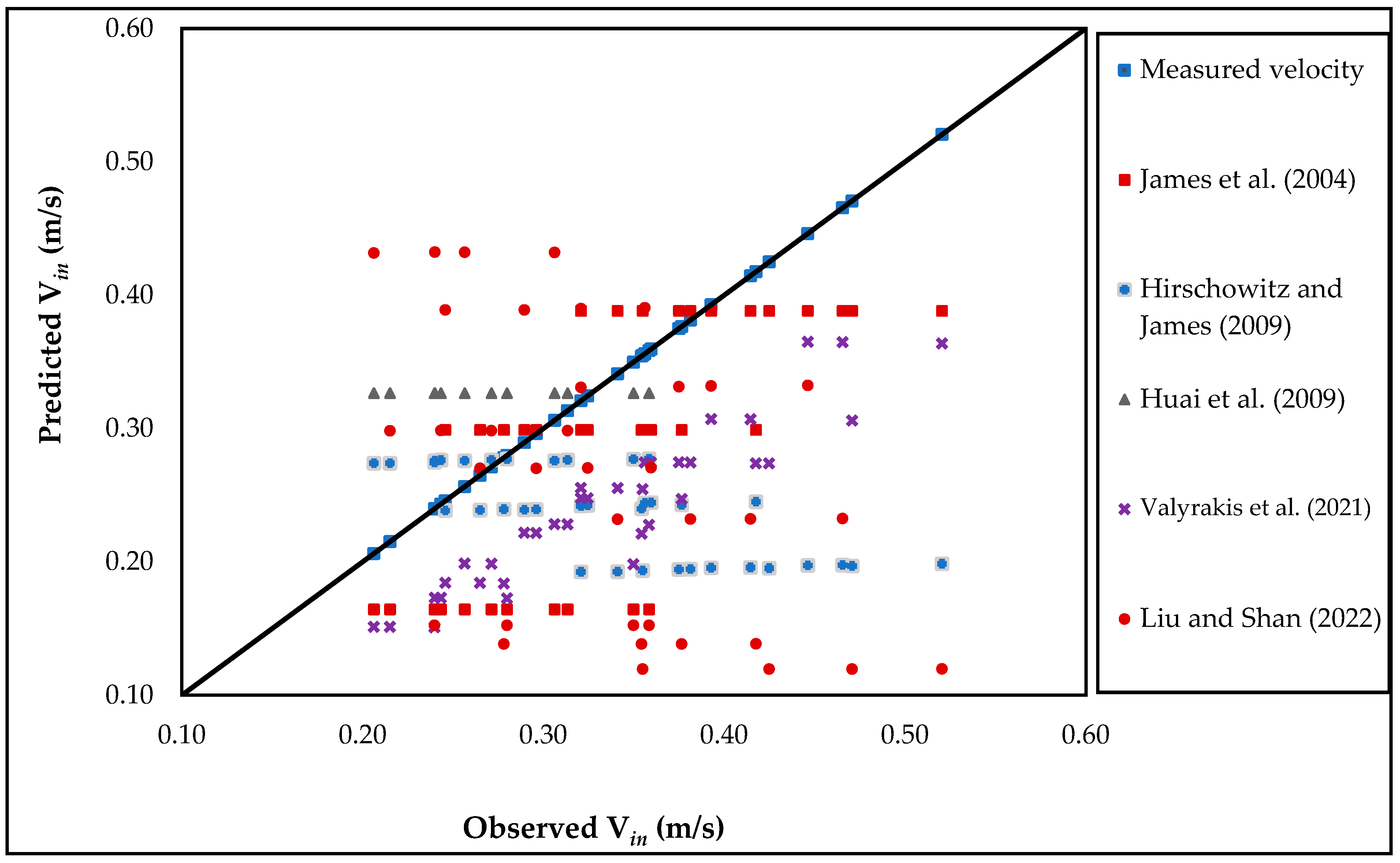
| Authors/Model | Average Error | Maximum Error | Minimum Error | Variance | RMSE |
|---|---|---|---|---|---|
| James et al. [16] | −0.189 | 0.080 | −0.043 | 0.018 | 0.080 |
| Hirschowitz and James [10] | −0.322 | 0.068 | −0.098 | 0.018 | 0.141 |
| Huai et al. [17] | −0.014 | 0.493 | 0.259 | 0.053 | 0.299 |
| Valyrakis et al. [14] | −0.165 | −0.055 | −0.095 | 0.019 | 0.100 |
| Liu and Shan [18] | −0.400 | 0.247 | −0.062 | 0.022 | 0.175 |
| λ | Fro | (Vu/u)max | (Vd/u)max | (Vin/u)max | /yo) | |
|---|---|---|---|---|---|---|
| λ | 1.00 | |||||
| Fro | 0.00 | 1.00 | ||||
| (Vu/u)max | 0.31 | 0.86 | 1.00 | |||
| (Vd/u)max | 0.55 | 0.72 | 0.93 | 1.00 | ||
| (Vin/u)max | 0.63 | 0.67 | 0.90 | 0.98 | 1.00 | |
| (/yo) | 0.37 | 0.71 | 0.73 | 0.73 | 0.72 | 1.00 |
| Term | Bilateral Weeds | Unilateral Weeds |
|---|---|---|
| Upstream relative velocity | ||
| Downstream relative velocity | ||
| Relative velocity inside the weedy patch | ||
| Relative maximum scour depth |
Disclaimer/Publisher’s Note: The statements, opinions and data contained in all publications are solely those of the individual author(s) and contributor(s) and not of MDPI and/or the editor(s). MDPI and/or the editor(s) disclaim responsibility for any injury to people or property resulting from any ideas, methods, instructions or products referred to in the content. |
© 2023 by the authors. Licensee MDPI, Basel, Switzerland. This article is an open access article distributed under the terms and conditions of the Creative Commons Attribution (CC BY) license (https://creativecommons.org/licenses/by/4.0/).
Share and Cite
Elzahry, E.F.M.; Eltoukhy, M.A.R.; Abdelmoaty, M.S.; Eraky, O.M.; Shaaban, I.G. Effect of Rigid Aquatic Bank Weeds on Flow Velocities and Bed Morphology. Water 2023, 15, 3173. https://doi.org/10.3390/w15183173
Elzahry EFM, Eltoukhy MAR, Abdelmoaty MS, Eraky OM, Shaaban IG. Effect of Rigid Aquatic Bank Weeds on Flow Velocities and Bed Morphology. Water. 2023; 15(18):3173. https://doi.org/10.3390/w15183173
Chicago/Turabian StyleElzahry, Elzahry Farouk M., Mahmoud Ali R. Eltoukhy, Mohamed S. Abdelmoaty, Ola Mohamed Eraky, and Ibrahim G. Shaaban. 2023. "Effect of Rigid Aquatic Bank Weeds on Flow Velocities and Bed Morphology" Water 15, no. 18: 3173. https://doi.org/10.3390/w15183173
APA StyleElzahry, E. F. M., Eltoukhy, M. A. R., Abdelmoaty, M. S., Eraky, O. M., & Shaaban, I. G. (2023). Effect of Rigid Aquatic Bank Weeds on Flow Velocities and Bed Morphology. Water, 15(18), 3173. https://doi.org/10.3390/w15183173