Article

Ice Phenology and Thickness Modelling for Lake Ice Climatology

by
Matti Leppäranta
Institute of Atmospheric and Earth Sciences, University of Helsinki, 00014 Helsinki, Finland
Water 2023, 15(16), 2951; https://doi.org/10.3390/w15162951
Submission received: 30 July 2023 / Revised: 12 August 2023 / Accepted: 14 August 2023 / Published: 16 August 2023
(This article belongs to the Special Issue Hydrophysical Parameters and Gases in Ice-Covered Lakes)

Abstract

:
Analytic methods are useful for lake ice climatology investigations that account for ice phenology, thickness, and extent. Ice climatology depends on the local climate and lake characteristics, which can be compressed into a few forcing factors for analytic modelling. The internal factors are lake depth, size, and water quality, while the external factors are solar radiation, air–lake interaction, and heat flux from bottom sediment. A two-layer temperature structure with a sharp thermocline in-between is employed for the water body and a non-inert conduction law for the ice cover. A thermal equilibrium approach results in temperature and ice thickness solutions, and a time scale analysis provides the applicability of the equilibrium method for lake ice climatology. A non-steady solution is needed for ice melting.

1. Introduction

The extent of freezing lakes in the Northern Hemisphere is from 30–35° N over the high Tibetan Plateau to the coast of the Arctic Ocean at 70–75° N. Ice cover is a seasonal phenomenon apart from a few polar and mountain lakes. Ice formation, growth, and breakup bring major changes to the physics, ecology, and human living conditions in districts of seasonally freezing lakes [1,2,3,4]. The thermal response of lakes depends on their depth, horizontal size, morphology, and water type, while the primary factors that drive the evolution of lake ice cover are the radiation balance, air–lake interaction, and heat exchange with the lake bottom [4,5,6,7]. The air–lake interaction has an impact also on the mass balance of lake ice. Climate variations show up strongly in lake ice conditions, and thus, lake ice seasons are sensitive indicators of climate [2,6,8]. In addition to ice phenology, the maximum annual ice thickness and maximum annual ice extent are the key long-term seasonal characteristics of lake ice cover.
Lake ice climatology has been investigated with time series analyses [6,9,10,11,12,13,14], mathematical modelling [15,16,17], and remote sensing [18,19,20]. A purely statistical approach has usually been taken in the time series analysis. The relation of time series statistics to physical lake processes and weather history is non-linear and contains time scales, so linear statistical inference may be misleading [14], e.g., a first-order physics approach to ice growth shows ice thickness scales with the square root of the freezing-degree days.
Mathematical lake ice models are forced using weather and heat flux from water to the ice bottom [16,21]. For climate studies, simple analytic or semi-analytic models are often feasible [14,17]. The models can be used to examine the physical basis of lake ice climatology and the climate sensitivity of the lake ice season characteristics for individual lakes or for regions up to the global scale. Modelling also aids in finding proper statistics for the ice time series analyses. These statistics are based on time integrals where the time scale depends on the lake size. Overall, the memory time scale of most lakes is less than 1 year so that interannual variations in ice climatology arise only from external sources.
First-order analytic models for ice phenology, thickness, and extent based on a passive lake water body were derived in [22]. The dependence of the lake ice season on air temperature was quantified, and the role of snow cover in ice growth and breakup was qualitatively illustrated. The work here is extended to an interactive, lake-ice–two-layer water body model. The purpose is to examine the role of the lake water body in the seasonal ice cycle, to analyse the scaling of the climate sensitivity of lake ice seasons, and to improve interpretation tools for time series analyses. A two-layer lake has two internal timescales in response to thermal forcing. Equilibrium conditions are applicable for temperature in shallow lakes and for ice thickness when the solar heat flux or the heat flux from water to the ice bottom is large, otherwise the lengths of the periods of water cooling and ice growth are restricting factors and a non-steady model is required.

2. Materials and Methods

2.1. Model Equations for Water Temperature

Most seasonally freezing lakes are dimictic. Summer warming and winter cooling produce the summer and winter stratification, while the overturning of the water mass takes place in autumn and spring. The stratification consists of three layers: the surface and bottom layers’ system and the thermocline layer between. The overturns cut the ice season from the annual cycle. Autumn overturn starts a “prewinter” (as called in [23]), when the lake may freeze in a short time, and spring overturn, which begins under ice and ends soon after breakup, overlaps the ice decay period.
Here, freshwater lakes are idealized as a two-layer system where the thermocline is taken as a sharp interface between the upper (surface) and lower (bottom) layers (Figure 1). In summer, the surface layer is warmer than the bottom layer, while in cold (a surface temperature below 4 °C) conditions, the stratification is inverse. The one-dimensional heat conduction law with the flux (Neumann) boundary condition is employed on top, and the flux or fixed (Dirichlet) boundary condition can be taken at the bottom [4,5,24]:
ρ w c w T t = z k w T z + Q s z
z = 0 : k w T z = Q 0
z = H : k b T z = Q b , o r   T = T b
where T is temperature; t is time, ρ w , c w , and k w are the density, specific heat, and thermal conductivity of water, respectively; z is the positive vertical coordinate positive up; Q s z is solar radiation at depth z ; Q 0 and Q b are the surface and bottom heat fluxes, respectively; H is depth; and k b and T b are the thermal conductivity and temperature at the bottom. The standard MKSA units are employed except that here, day (d) is a convenient unit of time.
Integrating across the upper and lower layers with the Neumann boundary conditions, we have equations for the layer temperatures T 1 and T 2 , surface forcing, and the stability condition of the layering:
d T 1 d t = λ a T a T 1 + λ 1 T 2 T 1 + f a
d T 2 d t = λ 2 T 1 T 2 + f b
Q 0 = K 0 + K 1 T a T 1
λ a = K 1 ρ w c w H 1 , λ 1 = k w ρ w c w H 1 , λ 2 = k w ρ w c w H 2 , f a = K 0 ρ w c w H 1 , f b = Q b ρ w c w H 2
ρ w T 2 > ρ w T 1 ; ρ w T = ρ w T m α T T m 2
where T a is air temperature, K 0 and K 1 are the parameters of the surface heat flux, H 1 and H 2 are the layer depths, H 1 + H 2 = H , T m = 3.98   is the temperature of the maximum density, and α 0.0083 kg m−3 °C−2 is the fit parameter of the quadratic density equation in (2e). The dimension of λ a ,   λ 1   a n d   λ 2 is inverse time, they are the inverse relaxation times in the system; and the dimension of f a   a n d   f b is temperature/time, they represent the surface and bottom heating rates. The surface heat flux parameters in general depend on time. K 0 is highly positive in the summer due to solar radiation while in the winter, it depends on latitude, and K 1 ~ 10 20 W m−2 °C−1 can be taken as fixed in the first approximation [17]. K 0 also depends on evaporation, and K 1 depends largely on wind speed.
In the case of the Dirichlet bottom boundary condition, we take
Q b = k b T b T 2 f b = λ b T b T 2 ,                 λ b = k b ρ w c w H 2
where k b is the heat exchange coefficient at the bottom, and λ b is one more inverse relaxation time in the system.
In the overturning periods, the water body is homogenous, T 1 = T 2 = T , and the layers can be added together for a one-layer model:
d T d t = λ a T a T + f a + f b
where the parameters λ a ,   f a ,   a n d   f b are defined with H 1   a n d   H 2 replaced by H . The one-layer model can also be used for the upper layer alone with the lower layer acting as a passive boundary condition.

2.2. Ice–Water Model

In the presence of ice cover on a lake surface, the surface water temperature is at the freezing point, and ice grows and melts in the interaction with the atmosphere and water body [4,5]. Ice cover is taken here as a rigid, static layer with thickness h , specified by its density and thermal conductivity without accounting for the type of ice crystal structure. The approach is feasible when congelation ice is the dominant type. The lower-layer-temperature Equations (2b,f) and stability criterion (2e) apply, and the upper layer temperature and ice thickness are obtained from
d T 1 d t = λ 1 T f + T 2 2 T 1 + f s
d h d t + a w T 1 T f = a i T f T 0 h = F 0
f s = δ Q s ρ w c w H 1 , a i = k i ρ i L f , a w = k w ρ i L f H 1 , F 0 = Q 0 ρ i L f
where δ Q s is the absorption of sunlight in the upper layer, T f is the freezing point temperature, ρ i is the density of ice, k i is the thermal conductivity of ice, and L f is the latent heat of freezing. During growth, T 0 < T f , while during melting, T 0 = T f . The time scales of ice growth are τ i = h 2 / a i T f T 0 and τ w = h / a w T 1 T f , while in ice melting, the time scales are τ w and h / F 0 .

3. Equilibrium

3.1. Temperature Equilibrium

The equilibrium solution of a two-layer system in an open-water situation is obtained from Equations (2a–f). For physically realizable conditions, the surface temperature is above the freezing point, and in the lower layer, the density must be larger than in the upper layer. Thus,
T 1 = T a + K 0 + Q b K 1 > T f , T 2 = T 1 + Q b k w
ρ w T 2 > ρ w T 1
The stability condition requires that T 2 T m < T 1 T m , i.e., the lower layer temperature is closer to the temperature of the maximum density. Thus, if Q b > 0   Q b < 0 , equilibrium is possible only for T 2 < 8   T 2 > 4   in fresh water. In an open-water situation, k w ~ 50 W m−2 °C−1 represents the turbulent thermal conductivity.
When T f < T 1 T m , the open-water equilibrium is possible for
T a > T f T , T = K 0 + Q b K 1
Apart from geothermal lakes, T ~ 1   in tundra lakes and T ~ 0   in boreal lakes but it can be several degrees positive in low-latitude alpine lakes [17]. Fluctuations of air temperature below the critical value must be shorter than the relaxation time λ a 1 = c H 1 ,   c 2.5 d m−1 to keep the open surface state.
In lake ice climatology, the freezing-degree days S   has been used as a predictor for the freezing date [25]. This can be physically motivated in mid-latitudes using the equilibrium model with S > T a λ a 1 , T a < T f , where · is the time averaging operator. If the air temperature is lower than the freezing point for longer than the relaxation time, freezing takes place. The connection with lake depth (parameter λ a 1 H 1 ) explains why deep lakes freeze over later (if at all) than shallow lakes in the same climate region. Also, one should examine the properties of air temperature time series more widely, not only the basic statistics but also autocorrelation, in studies of the freezing date.
Example 1.
In typical boreal lakes, scales in fall cooling at T 1 < T m are Q b ~ 5 W m−2, K 1 ~ 20   W m−2 °C−1, K 0 ~ 0 , and k w ~ 50   W   m 2   1 . Then, the equilibrium is T 1 = T a + 0.25   , T 2 = T 1 + 0.1   . The lake freezes at T a < T f 0.25   . The relaxation time is λ a 1 12.5 d.
The two-layer model can sometimes be reduced to the slab model (Equation (3)). When T 1 T m , T 2 T m , i.e., to a full turnover that may continue above or below T m in the presence of mechanically forced mixing. The equilibrium solution with the Dirichlet bottom boundary condition (Equation (2f)) is
T = ω a T a + 1 ω a T b + K 0 K 1 + k b > T f , ω a = K 1 K 1 + k b
We have a weighted average of air temperature and bottom temperature plus a shift 0 , which depends on the radiation balance and evaporation.

3.2. Ice Equilibrium

When there is ice cover, the equilibrium is
T 1 = T f + 1 k w δ Q s + Q b > T f
T 2 = T 1 + Q b k w > T 1
h e = k i T f T 0 δ Q s + Q b
The lower-layer temperature is formally as without ice (see Equation (5a)), while the top of the upper layer is forced by the freezing point temperature. For consistency, ice surface temperature is T 0 < T f , and for stability, Q b > 0 , as is the case normally in seasonal lakes. For Q b = 0 , the water body is isothermal at equilibrium, and if δ Q s = 0 as well, there is no equilibrium thickness, but the ice grows as long as T 0 < T f . For T 0 T f , the equilibrium thickness vanishes, i.e., h e 0 .
At freeze-over, mixing is strongly reduced, and the thermal conductivity of water decreases to k w ~ 10 W m−2 1 , at the extreme, down to the molecular value k w = 0.56 W m−2   1 . For k w ~ 10 W m−2 1 and Q b , δ Q s ~ 5   W m 2 , we have T 1 ~ T f + 1   ,   T 2 ~ T 1 + 0.5   . If T f T 0 = 10   , the equilibrium ice thickness is 2.1 m.
The time scale τ of ice thickness equilibrium can be large. Equation (4b) gives, after some manipulation,
τ = ρ i L f h e δ Q s + Q b = a i T f T 0 δ Q s + Q b / ρ i L f 2
For h e ~ ½ m, the heat flux from below must be more than 40 W m−2 to reach the equilibrium in 3 months. Thus, in typical conditions in boreal and tundra lakes, there is no climatic equilibrium state for ice thickness but only ice growth and melt periods. The growth period ends when the ice surface temperature settles to the melting point in late winter. In low-latitude, dry climate alpine lakes, a large fraction of sunlight penetrates the ice, making seasonal equilibrium possible [26].
Example 2.
For T f T 0 ~ 10   and δ Q s + Q b ~ 10 W m−2, we have h ~ 2.1 m. The time scale of ice growth is then almost 2 years. Then, at h ~ 1 m, the growth rate is 0.85 cm d−1. With low equilibrium thickness, the time scale is short, e.g., for δ Q s + Q b ~ 100 W m−2, the equilibrium thickness is 20 cm, and the time scale is 1 week.
An equilibrium between ice thickness and sublimation is possible. For sublimation rate E , the latent heat flux ρ i L f E can be added to the denominator in Equation (8c). This flux can be important in a dry and cold climate [27,28].
In the temperature equation, the stability condition requires that ρ T 1 ρ T f . In the case of solar forcing, the stability condition is T 1 < 8   or δ Q s > k w 8   T f ~ 80 W m−2. In the case of sediment heat flux, if T b > 8   and k b > 0 , the heating keeps on convection through all depths, resulting in an open-water situation.

4. Time Evolution

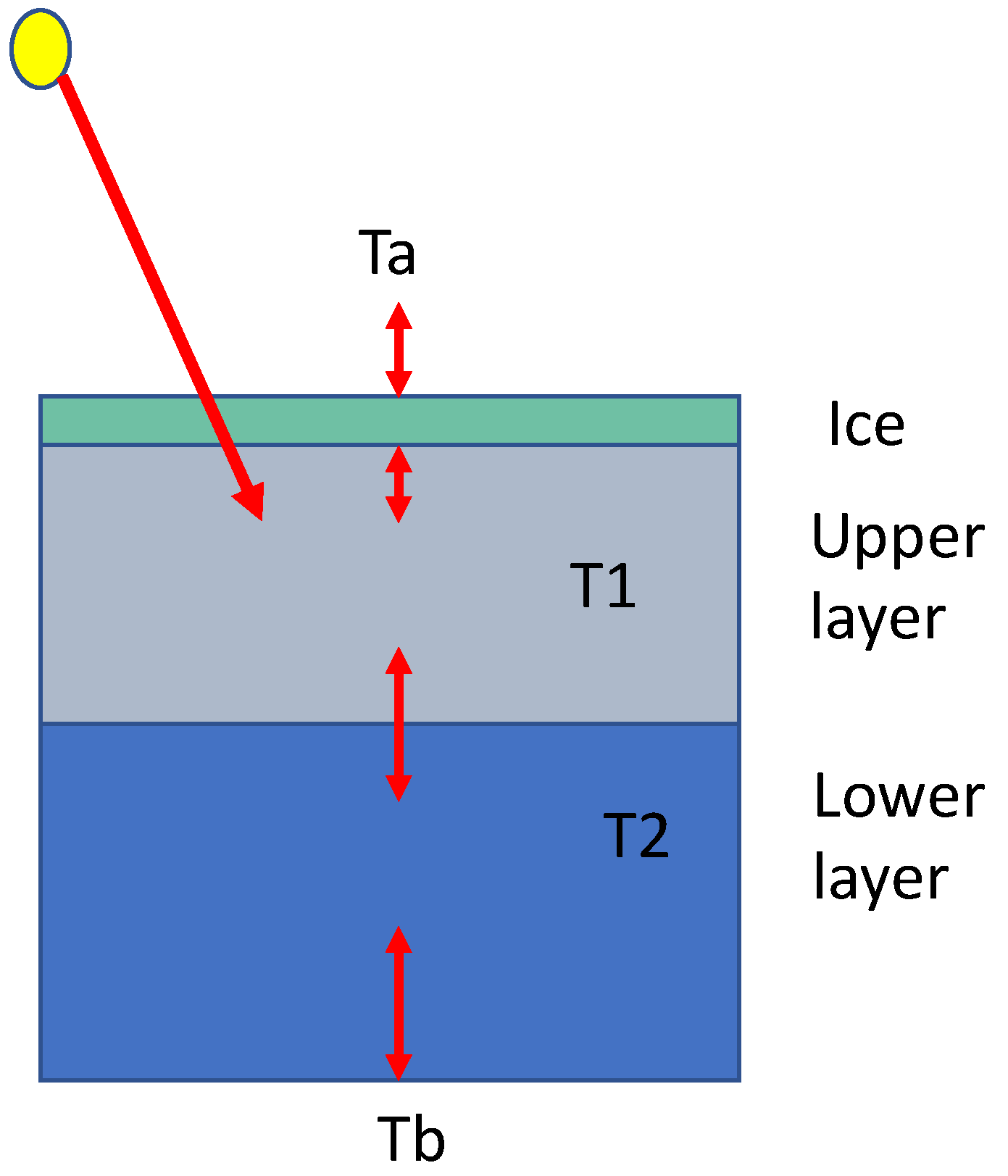
4.1. The Two-Layer System

The system forms a pair of ordinary linear differential equations that can be directly integrated, e.g., using the elimination method (see textbooks on ordinary differential equations). The homogeneous system
d T 1 d t = λ a T 1 + λ 1 T 2 T 1
d T 2 d t = λ 2 T 1 T 2
can be transferred into
d 2 T 1 d t 2 + λ a + λ 1 + λ 2 d T 1 d t + λ 2 λ a T 1 = 0
The solution is for the upper layer T 1 = A e r 1 t + B e r 2 t , where A   a n d   B   are constants depending on the initial conditions, and r 1,2 are the roots of the characteristic equation r 2 + λ a + λ 1 + λ 2 r + λ 2 λ a = 0 , i.e., the negative inverse time scales of the system:
r 1,2 = 1 2 λ a + λ 1 + λ 2 ± 1 4 λ a + λ 1 + λ 2 2 λ a λ 2
The lower-layer solution is then obtained directly from Equation (10a). Both roots in Equation (12) are real and negative (for r 1 “+” is taken in Equation (12)), and thus the solution disappears from the initial state with the time scales r k 1 . This also means that disturbances from an equilibrium disappear with these time scales. We have λ a , λ 1 H 1 1 ,   λ 2 H 2 1 . Usually, λ a λ 2 1 4 λ a + λ 1 + λ 2 2 , and
r 1 λ a λ 2 , r 2 λ a + λ 1 + λ 2 + λ a λ 2
When λ 2 λ a , λ 1 , or the lower layer is inert, r 1 0   a n d   r 2 λ a + λ 1 . In general, the values of the parameters λ a , λ 1 , λ 2   are of the order of 0.5 d−1 divided by depth in meters, with λ 1 / λ 2 = H 2 / H 1 .
Example 3.
For H 1 = H 2 = 10 m, we have λ a + λ 1 + λ 2 = 0.15 d−1, and r 1,2 1 = 52 d, 7.6   d. In a deep lake, H 1 = 10 m and H 2 = 50 m, and we have r 1,2 1 = 210   d ,   9.5 d. Thus, there is a rapid first adjustment of the upper layer followed by a slow adjustment of the whole system.
Starting with T 1 0 = T 2 0 = T 0 , we have the upper-layer solution
T 1 = r 1 + λ a r 1 r 2 e r 2 t r 2 + λ a r 1 r 2 e r 1 t T 0
It is seen that both terms in the brackets are positive and vanish at t . In the beginning, T 1 1 λ a t T 0 , and the second term disappears faster. In the example above, the solution is T 1 = 0.28 e r 2 t + 0.72 e r 1 t for H 1 = H 2 = 10 m and T 1 = 0.45 e r 2 t + 0.55 e r 1 t for H 1 = 10 m , H 2 = 50 m.
The general solution of the full model is obtained by adding a special solution, T 1 e , of the heterogeneous system to the homogeneous equation:
T 1 = A e r 1 t + B e r 2 t + T 1 e
When H 2 , then λ 2 0 and r 1 1 = , i.e., there is only the relaxation for the surface layer and the system is reduced to the slab model with λ 1 , T 2 being equivalent to λ b , T b . Then, the solution, using the Dirichlet boundary condition at the bottom and ignoring the transient terms, is as follows:
T t = t e λ t τ λ a T a + T R + λ b T b d τ
where λ = λ a + λ b . If T R = K 0 / K 1 and T b are constant, we have
T t = t e λ t τ λ a T a τ d τ + λ a λ T R + λ b λ T b
The solution includes a weighted integral of past air temperature and a fixed shift, which depends on the radiation balance and heat flux from the lake bottom. The relaxation time of the system is λ 1 H . Whether the lake freezes, i.e., T = T f , depends on the air temperature integral and the shift terms, and the freezing date can be formally expressed as t F = t F H , w T a , T R , T b , where the integral refers to the weighted ( w ) air temperature history.
The growth of ice extent A ,   0 A A L , where A L is the area of the lake, follows the hypsographic curve Γ H equal to the fractional area deeper than H , i.e., Γ 0 = lake area and Γ H = 0   for H > H m a x . At depth H , the lake freezes at time t F = t F H , and the ice extent is a function of weather and hypsographic-curve lakes [14]. The evolution of the ice extent therefore follows the formula
d A d t = d Γ / d H d t F / d H
For example, if both the hypsographic curve and freezing date are linear, and Γ H = 1 H / H m a x and t F H = t F 0 + α H , we have A = α H m a x 1 t t F 0 . If α ~ 0.5 d m−1 and H m a x = 30 m, ice extent increases by 6.7% per day and reaches 100% 15 days after first freezing at the shore. The solution is sensitive to the initial freezing date t F 0 , which depends on the air temperature evolution, e.g., in Lake Ladoga, where the mean and maximum depths are 48 m and 210 m, it takes an average of 58 days to reach the complete ice coverage [14].

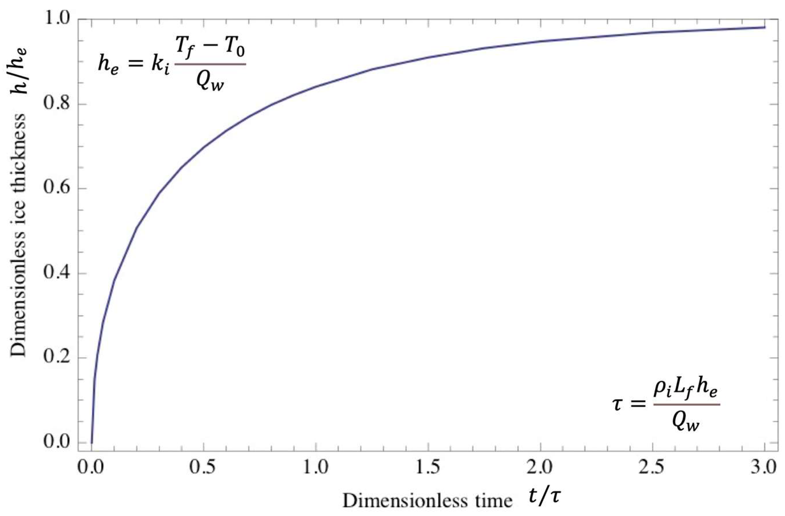
4.2. Ice-Cover Thickness

Ice growth forms a nonlinear system, which interacts with the water body and atmosphere. The heat flux from water to ice can, at the extreme, create a permanent opening in the ice cover, or provide an equilibrium where the heat flux through ice ( h > 0 ) equals the heat flux from the water. The general case of ice thickness in the presence of heat flux from water cannot be solved analytically, but special conditions can be worked through.
When the surface temperature T 0 and heat flux from water Q w are constant, the ice growth problem (Equation (4b)) can be solved in an implicit form:
h h e + log 1 h h e = t τ ; h e = k i T f T 0 Q w , τ = ρ i L f h e Q w
where h e is the equilibrium ice thickness, and τ is the time scale of ice growth. The solution is shown in Figure 2. When h h e , the left-hand side is approximately 1 2 h h e 2 and the ice grows in proportion to the square root of time with a minor influence from the heat flux from water. Furthermore, h = h e / 2 at t / τ = log 2 1 / 2 0.193 .
The growth rate decreases with time and ice thickness approaches the equilibrium asymptotically, e.g., for T f T 0 = 10   and Q w = 10 W m−2, we have h e = 2.1 m. The time scale is τ 2 years, and the thickness is half of the equilibrium or 1.05 m at t = 0.193 · τ ≈ 140 days. For Q w = 0 ,   h e = , and in 140 days, the ice would grow to 1.2 m.
The warming of the surface water with penetrated solar radiation δ Q s can be simply added to the heat flux Q w . Since δ Q s = Q s 0 e κ h , where Q s 0 is the net solar radiation at the surface and κ is the light attenuation coefficient, there is an additional coupling effect. The solution of Equation (18) for the time evolution is no more possible, but, ignoring Q w , we have an implicit formula for the equilibrium thickness and time scale:
h e e κ h e = k i T f T 0 Q s 0 , τ = e κ h e h e ρ i L f Q s 0
For transparent ice ( κ = 0 ), we have thin ice at equilibrium due to strong bottom melting and a short time scale. With increasing attenuation, both the thickness and time scale increase.
The case of periodic heat flux, Q w = ρ i L f q w 1 + sin Ω t , where ρ i L f q w and Ω are, respectively, the amplitude (and average) and frequency of Q w , can be solved for small-thickness amplitude situations, h = h e + e ,   e h e , using the perturbation technique. The thickness of ice follows the forcing cycle with the same frequency and with the amplitude and phase shift of
e = q w ω 2 + η 2 , φ = arctan ω η , η = k i T f T 0 ρ i L f h e 2
If q w = 1 cm d−1 (a very high amplitude, corresponding to Q w 35 W m−2) and T f T 0 = 10   , then h e = 60 cm and η = 2.16 month−1. For a daily cycle, we have e = 0.11 cm and η = 0.017 rad, while for a monthly cycle, e = 3.4 cm and η = 0.50 rad. The phase shift is nearly π / 2 rad or 6 h in the first case, and it is 1.49 rad or 7.1 d in the second case.
The melting of ice is a heat flux problem where the solar radiation parameters have a key role due to their large space–time variability [29]. At the melting stage, T 0 = T f , and solar radiation heats the ice from the top, inside, and bottom. The melting equation is
d h d t = a w T 1 T f + Q 0 + Q s i
where Q 0 is the surface heat balance with only the infrared band of solar radiation included, and Q s i is the absorption of solar radiation by the ice. The radiation penetrating the ice cover, δ Q s , is used for heating the water temperature and therefore increasing the heat flux a w T 1 T f . This partition needs parameterizations of albedo and the light attenuation coefficient that has a lot of freedom in the perspective of available data [4].

5. Discussion

Slab models have been used for lake thermodynamics for a long time. They are easy to treat with analytic methods and applicable for shallow lakes. Beneath ice, turbulence is weak or absent, and in analytic modelling, the heat flux from water to ice has been based on a molecular conduction approach or on molecular analogue parametrization schemes [4]. In two-layer modelling, the interaction between upper and lower layers can be accounted for; the lower layer can also be made to represent the bottom sediment.
A method to predict the freezing date based on the weighted sum of past daily air temperatures was derived in [30], with more weight on more recent days. This was extended in [22] with an advanced parametrization of the surface heat flux. This model can be used to predict the climate sensitivity of the freezing date, but the weighted air temperature integral cannot be converted to freezing-degree days, which is usually employed in a time series analysis [2,25]. It was seen in Section 3.1 that an equilibrium condition during a cold spell can predict the freezing event based on the freezing-degree days, but due to the time scale limitation, it is applicable only under a shallow depth or mixed layer condition.
Ice growth follows freezing-degree days, as has been known for a long time [5,10,21]. In this work, it was shown that ice thickness may reach equilibrium in the winter, when the heat flux from water to the bottom of ice is large. The source of this heat can be deep water, bottom sediment, or solar radiation penetrated through the ice cover. When this heat flux is small, the time scale of equilibrium is longer than the annual ice seasonal. For perennial lake ice, such as that found in the Antarctic continent [31], an annual equilibrium may exist between solar radiation and ice thickness, as shown in Section 4.2.
The relaxation time parameters lead to the time scales in the system. λ a depends on the atmospheric surface layer and is therefore independent of λ 1   a n d   λ 2 . The parameters λ 1   a n d   λ 2 are inversely proportional to the thicknesses of, respectively, the upper and lower layers, i.e., λ 1 / λ 2 = H 2 / H 1 . Thus, in deep lakes, λ 1 λ 2 . As seen in the definition, they depend on the density, specific heat, and thermal conductivity of water. When the lower layer represents the sediment, the properties of λ 2 must represent the sediment. For a wet sediment layer, the heat storage can be large, and the water properties work in the first approximation, with the molecular value for the conductivity that makes λ 2 small. In an open-water environment, the sediment heat flux usually has a minor impact, but it can be important in the ice season.
The surface forcing function Q 0 = K 0 + K 1 T a T 1 contains zeroth order radiation balance and evaporation/sublimation in K 0 and the first-order correction for the temperature difference T a T 1 in K 1 [17]. K 0 has a strong annual cycle with K 0 ~ 100 W m−2 in the summer and K 0 ~ 50 W m−2 in the winter; while K 1 is more stable, K 1 ~ 10 W m−2 °C−1 is strictly positive in practice. The ratio K 0 / K 1 adds a term in the solution of the surface temperature; at K 0 / K 1 = 0 , the upper-layer temperature equals a low-pass-filtered air temperature, while for large K 0 / K 1 , the situation is dominated by the radiation balance.
The present work treated dimictic freshwater lakes. Most freezing lakes fit in this category. As such, the results are applicable to monomictic lakes, and for polymictic lakes, the special one-layer case is feasible. Accounting for the breakage of ice with wind would necessitate adding a mechanical model to the system that would be useful especially in large lakes. In regards to salinity, firstly, its influence on the water density may be reflected in the stratification, and when preventing deep convection, the salinity may even support ice-cover formation. Secondly, the freezing point is lowered with a direct consequence on the freezing date, and the decrease in the temperature of the maximum density has an impact on the mixing conditions.

6. Concluding Remarks

Analytic methods are useful for lake ice climatology investigations. Ice phenology and properties depend on the local climate and lake characteristics, which can be compressed into a few internal and forcing factors for analytic modelling. The forcing factors considered are solar radiation, air–lake interaction, and heat flux from bottom sediment, while ice climatology contains ice phenology, thickness, and extent.
A two-layer temperature structure is employed for the water body and a non-inert conduction law for the ice cover. The thermal equilibrium approach results in temperature and ice thickness solutions, and the time scale analysis provides the applicability of the equilibrium method for lake ice climatology. The non-steady solution is applied for ice melting. The two-layer approach provides a basic framework for understanding the ice–water coupling in thermodynamics of freezing lakes. Prior to freezing, the inverse stratification of the water body forms with the thermocline depth depending on the forced mixing conditions. Beneath ice cover, a stable inverse stratification prevails until solar radiation starts spring convection.
The solution of the equilibrium conditions and the time scales was illustrated. Solving for the full-time evolution brings complexity to the interpretation of the two-layer model outcome, while with ice cover, included analytic solutions are possible only in restricted cases. Also, for a lake ice climatology analysis based on time series, higher-order statistics of air temperature would be useful due to nonlinearities in the progress of ice seasons. A forthcoming paper will introduce applications to a time series analysis of lake ice climatology.

Funding

This research received no funding.

Data Availability Statement

This research does not include new data but is theoretical and the data used has been taken from the cited publications.

Acknowledgments

Comments of two anonymous reviewers are greatly appreciated, and this journal MDPI is thanked for supporting page charges.

Conflicts of Interest

The author declares no conflict of interest.

References

  1. Salonen, K.; Leppäranta, M.; Viljanen, M.; Gulati, R. Perspectives in winter limnology: Closing the annual cycle of freezing lakes. Aquat. Ecol. 2009, 43, 609–616. [Google Scholar] [CrossRef]
  2. George, G. (Ed.) Climate Change Impact on European Lakes; Springer: Berlin/Heidelberg, Germany, 2009. [Google Scholar]
  3. Knoll, L.B.; Sharma, S.; Denfeld, B.A.; Flaim, G.; Hori, Y.; Magnuson, J.J.; Straile, D.; Weyhenmeyer, G. Consequences of lake and river ice loss on cultural ecosystem services. Limnol. Oceanogr. Lett. 2019, 4, 119–131. [Google Scholar] [CrossRef]
  4. Leppäranta, M. Freezing of Lakes and the Evolution of Their Ice Cover, 2nd ed.; Springer-Praxis: Heidelberg, Germany, 2023. [Google Scholar]
  5. Ashton, G. Freshwater ice growth, motion, and decay. In Dynamics of Snow and Ice Masses; Colbeck, S., Ed.; Academic Press: New York, NY, USA, 1980; pp. 261–304. [Google Scholar]
  6. Sharma, S.; Blagrave, K.; Magnuson, J.J.; O’Reilly, C.M.; Oliver, S.; Batt, R.D.; Magee, R.M.; Straile, D.; Weyhenmeyer, G.A.; Winslow, L.; et al. Widespread loss of lake ice around the Northern Hemisphere in a warming world. Nat. Clim. Chang. 2019, 9, 227–231. [Google Scholar] [CrossRef]
  7. Noori, R.; Woolway, R.I.; Saari, M.; Pulkkanen, M.; Kløve, B. Six decades of thermal change in a pristine lake situated north of the Arctic Circle. Water Resour. Res. 2022, 58, e2021WR031543. [Google Scholar] [CrossRef]
  8. Noori, R.; Bateni, S.M.; Saari, M.; Almazroui, M.; Torabi Haghighi, A. Strong warming rates in the surface and bottom layers of a boreal lake: Results from approximately six decades of measurements (1964–2020). Earth Space Sci. 2022, 9, e2021EA001973. [Google Scholar] [CrossRef]
  9. Magnuson, J.J.; Robertson, D.M.; Benson, B.J.; Wynne, R.H.; Livingstone, D.M.; Arai, T.; Assel, R.A.; Barry, R.G.; Card, V.; Kuusisto, E.; et al. Historical trends in lake and river ice cover in the northern hemisphere. Science 2000, 289, 1743–1746, Erratum in Science 2001, 291, 254. [Google Scholar] [CrossRef] [PubMed]
  10. Korhonen, J. Long-term changes in lake ice cover in Finland. Nord. Hydrol. 2006, 37, 347–363. [Google Scholar] [CrossRef]
  11. Livingstone, D.; Adrian, R. Modeling the duration of intermittent ice cover on a lake for climate-change studies. Limnol. Oceanogr. 2009, 54, 1709–1722. [Google Scholar] [CrossRef]
  12. Bernhardt, J.; Engelhardt, C.; Kirillin, G.; Matschullat, J. Lake ice phenology in Berlin-Brandenburg from 1947–2007: Observations and model hindcasts. Clim. Chang. 2011, 112, 791–817. [Google Scholar] [CrossRef]
  13. Efremova, T.; Palshin, N. Ice phenomena terms on the water bodies of northwestern Russia. Meteorol. Hydrol. 2011, 36, 559–565. [Google Scholar] [CrossRef]
  14. Karetnikov, S.; Leppäranta, M.; Montonen, A. Time series over 100 years of the ice season in Lake Ladoga. J. Great Lakes Res. 2017, 43, 979–988. [Google Scholar] [CrossRef]
  15. Mironov, D.; Ritter, B.; Schulz, J.-P.; Buchhold, M.; Lange, M.; MacHulskaya, E. Parameterisation of sea and lake ice in numerical weather prediction models of the German Weather Service. Tellus A Dyn. Meteorol. Oceanogr. 2012, 64, 17330. [Google Scholar] [CrossRef]
  16. Yang, Y.; Leppäranta, M.; Li, Z.; Cheng, B. An ice model for Lake Vanajavesi, Finland. Tellus A 2012, 64, 17202. [Google Scholar] [CrossRef]
  17. Leppäranta, M.; Wen, L. Ice phenology in Eurasian lakes over spatial location and altitude. Water 2022, 14, 1037. [Google Scholar] [CrossRef]
  18. Wang, J.; Bai, X.; Hu, H.; Clites, A.; Holton, M.; Lofgren, B. Temporal and spatial variability of Great Lakes ice cover, 1973–2010. J. Clim. 2012, 25, 1318–1329. [Google Scholar] [CrossRef]
  19. Murfitt, J.; Duguay, C.R. 50 years of lake ice research from active microwave remote sensing: Progress and prospects. Remote Sens. Environ. 2021, 264, 112616. [Google Scholar] [CrossRef]
  20. Wang, X.; Qiu, Y.; Zhang, Y.; Lemmetyinen, J.; Cheng, B.; Liang, E.; Leppäranta, M. A lake ice phenology dataset for the Northern Hemisphere based on passive microwave remote sensing. Big Earth Data 2021, 6, 401–419. [Google Scholar] [CrossRef]
  21. Stepanenko, V.M.; Repina, I.A.; Ganbat, G.; Davaa, G. Numerical simulation of ice cover in saline lakes. Izv. Atmos. Ocean. Phys. 2019, 55, 129–139. [Google Scholar] [CrossRef]
  22. Leppäranta, M. Interpretation of statistics of lake ice time series for climate variability. Hydrol. Res. 2014, 45, 673–684. [Google Scholar] [CrossRef]
  23. Kirillin, G.; Leppäranta, M.; Terzhevik, A.; Bernhardt, J.; Engelhardt, C.; Granin, N.; Golosov, S.; Efremova, T.; Palshin, N.; Sherstyankin, P.; et al. Physics of seasonally ice-covered lakes: Major drivers and temporal/spatial scales. Aquat. Ecol. 2012, 74, 659–682. [Google Scholar]
  24. Sahlberg, J. A hydrodynamical model for calculating the vertical temperature profile in lakes during cooling. Nord. Hydrol. 1983, 14, 239–254. [Google Scholar] [CrossRef]
  25. Thompson, R.; Price, D.; Cameron, N.; Jones, V.; Bigler, C.; Catalan, J.; Rosén, P.; Hall, R.I.; Weckström, J.; Korhola, A. Quantitative calibration of remote mountain lake sediments as climate recorders of ice-cover duration. Arct. Antarct. Alp. Res. 2005, 37, 626–635. [Google Scholar] [CrossRef]
  26. Cao, X.; Lu, P.; Leppäranta, M.; Arvola, L.; Huotari, J.; Shi, X.; Li, G.; Li, Z. Solar radiation transfer for an ice-covered lake in the central Asian arid climate zone. Inland Waters 2020, 11, 89–103. [Google Scholar] [CrossRef]
  27. Huang, W.F.; Li, Z.; Han, H.; Niu, F.; Lin, Z.; Leppäranta, M. Structural analysis of thermokarst lake ice in Beiluhe Basin, Qinghai–Tibet Plateau. Cold Reg. Sci. Technol. 2012, 72, 33–42. [Google Scholar] [CrossRef]
  28. Leppäranta, M.; Lindgren, E.; Arvola, L. Heat balance of supraglacial lakes in the western Dronning Maud Land. Ann. Glaciol. 2016, 57, 39–46. [Google Scholar] [CrossRef]
  29. Leppäranta, M.; Lindgren, E.; Wen, L.; Kirillin, G. Ice cover decay and heat balance in Lake Kilpisjärvi in Arctic tundra. J. Limnol. 2019, 78, 163–175. [Google Scholar] [CrossRef]
  30. Rodhe, B. On the relation between air temperature and ice formation in the Baltic. Geogr. Ann. 1952, 1–2, 176–202. [Google Scholar]
  31. Hodgson, D.A. Antarctic lakes. In Encyclopedia of Lakes and Reservoirs; Bengtsson, L., Herschy, R.W., Fairbridge, R.W., Eds.; Springer: Berlin/Heidelberg, Germany, 2012; pp. 26–31. [Google Scholar]
Figure 1. A sketch of the model structure. Red arrows are for heat transfer; yellow disc is the Sun.
Water 15 02951 g001
Figure 2. A plot of dimensionless ice thickness vs. dimensionless time illustrating the influence of heat flux from the water body Q w on ice growth. Ice thickness approaches the asymptotic equilibrium thickness h e with time proportional to h e / Q w .
Water 15 02951 g002
Disclaimer/Publisher’s Note: The statements, opinions and data contained in all publications are solely those of the individual author(s) and contributor(s) and not of MDPI and/or the editor(s). MDPI and/or the editor(s) disclaim responsibility for any injury to people or property resulting from any ideas, methods, instructions or products referred to in the content.

