Abstract
Building robust age–depth models to understand climatic and geologic histories from coastal sedimentary archives often requires composite chronologies consisting of multi-proxy age markers. Pollen chronohorizons derived from a known change in vegetation are important for age–depth models, especially those with other sparse or imprecise age markers. However, the accuracy of pollen chronohorizons compared to other age markers and the impact of pollen chronohorizons on the precision of age–depth models, particularly in salt marsh environments, is poorly understood. Here, we combine new and published pollen data from eight coastal wetlands (salt marshes and mangroves) along the Atlantic Coast of the United States (U.S.) from Florida to Connecticut to define the age and uncertainty of 17 pollen chronohorizons. We found that 13 out of 17 pollen chronohorizons were consistent when compared to other age markers (radiocarbon, radionuclide 137Cs and pollution markers). Inconsistencies were likely related to the hyperlocality of pollen chronohorizons, mixing of salt marsh sediment, reworking of pollen from nearby tidal flats, misidentification of pollen signals, and inaccuracies in or misinterpretation of other age markers. Additionally, in a total of 24 models, including one or more pollen chronohorizons, increased precision (up to 41 years) or no change was found in 18 models.
1. Introduction
The last millennium contains major environmental changes that are important for understanding how the Earth may respond to future perturbations [1,2,3]. Environmental changes include natural climatic changes from the Medieval Climate Anomaly to the Little Ice Age (LIA) [4,5] and the onset of modern anthropogenically-driven climate and land use changes [6,7].
A robust, highly resolved geochronology in sedimentary archives is critical to constrain the timing of major environmental changes during the last millennium [8]. Every significant advance in geochronology has produced a paradigm-shifting breakthrough in our understanding of environmental changes from proxy records [9]. The geochronology of proxy records of environmental change from ~50 ka to present is commonly constrained using radiocarbon dating [10,11,12]. However, radiocarbon results dating to the last few centuries often yield age estimates with multiple distinct ranges due to the highly variable relative concentration of radiocarbon in the atmosphere. For example, variations in the atmospheric 14C/12C ratio from changes in solar activity (e.g., minima in 1500, 1700, and 1815 CE) [13] and combustion of radiocarbon-free fossil fuels primarily since the 1960s (known as the Suess effect) [14,15,16], cause some samples to have multiple potential age-ranges [17,18]. The last few hundred years of sediment-based proxy records can also be dated using a composite chronology including short-lived radioisotopes, such as 210Pb [19,20,21,22] and 137Cs [23,24], and anthropogenic pollution markers [25,26,27] (Figure 1). However, there are limitations imposed by sedimentary processes, sampling, and analytical factors of 210Pb, which can generate erroneous ages [28,29]. Pollution markers of trace metals are available after the regional onset of industrial activity [30,31,32] but are absent or unknown in many regions [33,34,35].
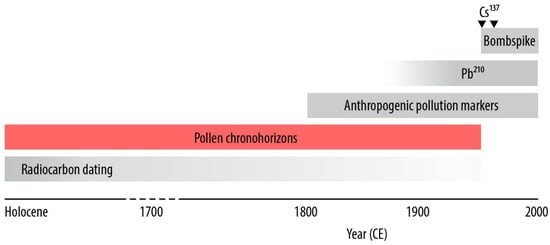
Figure 1.
Conceptual diagram of dating techniques and their age ranges highlighting the potential chronological gap between radiocarbon dating and pollution markers that pollen chronohorizons may circumvent.
The radiocarbon calibration plateaus and oscillations that occur between 1500 and 1950 CE and the limitations of short-lived radioisotopes and pollution markers make dating phenomena like the LIA and the onset of anthropogenically-driven climate change uncertain [17]. Pollen evidence of land-use changes that occurred during European settlement along the U.S. Atlantic Coast [36,37] provides chronohorizons that can improve the precision of age–depth models by filling this age-uncertainty gap [38,39,40]. Because fossil pollen is readily preserved in coastal, lacustrine, and salt and freshwater marsh sediments, pollen chronohorizons are applied in a variety of paleoclimate [41], relative sea level [42], and storm [43] reconstructions. Pollen chronohorizons are derived from changes in the relative abundance of pollen of certain plant taxa [36,44,45]. For example, a deforestation chronohorizon can be estimated from a decrease in arboreal pollen and a simultaneous increase in ragweed (Ambrosia) [36]. The ages of chronohorizons are estimated from personal journals, letters, and almanacs that contain information about specific changes in vegetation [25,26,40]. However, many of the ages associated with the chronohorizons have unknown uncertainties due to variations in the transport and preservation of pollen in the sedimentary record [46]. Additionally, applying chronohorizons to broad regions may be hampered by hyperlocality, that is, vegetation changes that are restricted to a specific location by dispersal mechanisms [47].
Here, we have collected published and unpublished pollen and chronology data (e.g., radiocarbon, 137Cs and pollution horizons) from sediment cores collected from eight coastal wetlands (salt marshes and mangroves) along the U.S. Atlantic Coast. Coastal wetlands are ecologically and economically important environments [48], which are under threat from sea-level rise, storm surges, and eutrophication [49,50,51,52]. We investigated the applicability of pollen chronohorizons from salt marsh and mangrove environments that have been studied using a consistent methodology for dating, sediment sampling, and analysis [27,42,53]. We documented eight unique pollen chronohorizons with up to three chronohorizons per study site (17 chronohorizons in total). We compared pollen chronohorizons to other age markers (radiocarbon, 137Cs, and pollution markers) to examine their consistency with other markers and their influence on the precision of age–depth models. We applied a Bayesian age–depth framework (Bchron) [54], which illustrated that 13 out of 17 ages assigned to individual pollen chronohorizons were consistent when compared with dates derived using other age markers. Inconsistencies are likely due to hyperlocality, sediment mixing, misinterpretation of pollen signals, and/or incorrect pollution and radiocarbon dates. We show that the greatest influence on the precision of age models occurred at coastal wetland sites with limited chronological data, highlighting the importance of pollen chronohorizons and providing a better understanding of age–depth modeling in these critical coastal environments.
2. Study Sites
We compiled pollen and chronological data from eight coastal wetlands (Figure 2a, Table 1). We include four published records (New York, New Jersey, North Carolina, and northern Florida) (Appendix A) and four newly analyzed records with unpublished chronological data (Connecticut, Delaware, Maryland, and southern Florida) (Table 2). Full site descriptions of the published and unpublished records can be found in the original publications and Appendix B, respectively.
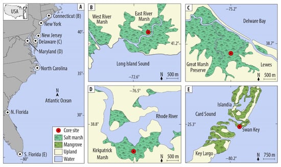
Figure 2.
Map of U.S. Atlantic Coast (A) showing the relative location of eight published and unpublished study sites, as well as individual site maps for Connecticut (B), Delaware (C), Maryland (D), and Southern Florida (E). Maps of other sites can be found in the original publications.

Table 1.
Site Descriptions. Regional vegetation identified using [55]. The site description and chronology related to other age markers can be found in the original publication.
Table 2.
Chronological data for unpublished sites. UMV refers to lead (Pb) pollution originating from the Upper Mississippi Valley. Core date refers to the year that the core was collected. Years before present is abbreviated as YBP with “present” defined at 1950.
Köppen climate zones for the sites span from humid continental to tropical savanna [59]. The tidal range of the study sites varies from 0.18 m in New Jersey [57] to 2.44 m in New York [56]. Sites have been influenced by anthropogenic activities, which have altered the plant communities and, therefore, the pollen assemblages. For example, ditching was common in many of our sites to drain the marsh [60,61,62,63]. Deforestation for agriculture and wood supply varied in time but was common to all of our sites [26,44,64] and is commonly used as a pollen chronohorizon [36]. Agricultural activities and importation of exotic plants such as the introduction of Casuarina in Florida [65,66], can also be recorded in pollen records.
3. Materials and Methods
3.1. Sediment Sampling
We selected sediment cores or trenches for extraction following detailed stratigraphic surveys of the underlying stratigraphy at each site. We recovered each core in overlapping, 50-cm long sections using an Eijelkamp Russian-type peat sampler [67]. In Connecticut, sediment samples were recovered from an excavated trench [53]. All cores and trench samples were placed in rigid plastic sleeves, wrapped in plastic film, and kept refrigerated until processing in the laboratory to minimize desiccation and/or decay. One core/trench section from each site was selected for detailed analysis that was representative of the site stratigraphy and was deemed most likely to produce a near-continuous reconstruction of vegetation change over the last 500 years. Site stratigraphy consisted of continuous salt marsh peat or mangrove peat throughout the studied sections.
3.2. Chronology
3.2.1. Pollen Processing and Analysis
The processing procedure for published studies can be found in the original publications. The unpublished studies followed a similar procedure. In Connecticut, Delaware, Maryland, and southern Florida, pollen sampling was performed at 4 cm intervals. Extraction of pollen and preparation of slides followed the methods outlined in Faegri and Iversen [68] and Bernhardt and Willard [40]. Between 100 and 500 hundred grains were counted.
We found eight unique pollen chronohorizons based on review of proposed reference dates in the literature, with up to three chronohorizons observed in each study site, producing a total of 17 chronohorizons (Figure 3). Table 3 includes detailed information regarding pollen changes and estimations of their age and associated uncertainty. We subsequently produced 24 age–depth models for the eight study sites: 17 site-specific models using individual pollen chronohorizons combined with other types of age markers and seven site-specific models with multiple pollen chronohorizons combined with other types of age markers.
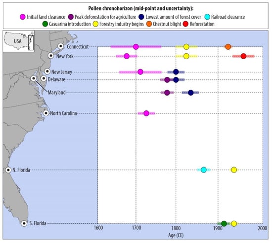
Figure 3.
Timing of pollen chronohorizons documented in the literature at each study site. Pollen data from published sites are available in the original publications.
Table 3.
Site pollen chronohorizons, their ages, and the ages predicted by NP Bchron model. 1a to 3b refers to the pollen chronohorizon identifier, with the numerical portion of the identifier designating the type of chronohorizon: (1) land clearance; (2) reforestation; and (3) introduction and loss of taxa, and the letter portion designating the specific chronohorizon (e.g., Chestnut blight). (Figure 4, Appendix C).
The eight unique pollen chronohorizons and their criteria for identification varies among the study sites. Pollen chronohorizons vary in whether they are qualitative (i.e., based on increases or decreases in abundance) or semi-quantitative (i.e., a numerical change or presence/absence) and whether the signal is local or regional. Uncertainty ranges of pollen chronohorizons are qualitative because they are estimates of the time-lag for vegetation changes to be recorded in the sedimentary record. The eight pollen chronohorizons can be grouped into three types: land clearance; reforestation; and introduction and loss of taxa (Table 3).
3.2.2. Radiocarbon
We performed radiocarbon analyses at all unpublished sites on identifiable plant macrofossils from sediment cores using the National Ocean Sciences Accelerator Mass Spectrometry (NOSAMS) facility at Woods Hole. At all sites, we extracted plant macrofossils (e.g., Spartina and Juncus) to reduce risk of older or younger contamination in bulk sediments, and selected surface markers likely to be in situ. We removed contaminating materials, such as extraneous particles, from the plant macrofossils by cleaning the specimen under a dissection microscope [57]. The radiocarbon samples also underwent acid-base-acid pretreatment prior to analysis to further remove contaminants [57]. Radiocarbon ages from NOSAMS were calibrated in Bchron using IntCal13 calibration data set [12,81]. Radiocarbon chronologies of published studies are found in the original publications (Table 1). Radiocarbon chronologies and Bchron-calibrated age ranges of unpublished studies are found in Table 2.
3.2.3. Radionuclide 137Cs
The fallout radionuclide 137Cs (t1/2 = 30.2 years) has been extensively used to provide estimates of age with depth in a sediment column. 137Cs is an artificially produced radionuclide present in the environment due to atmospheric fallout from atmospheric nuclear weapons testing, reactor accidents, and discharges from nuclear facilities. Global dispersion and fallout of 137Cs began in 1954 CE following the detonation of high-yield thermonuclear weapons with a distinct maximum in fallout in 1963 CE [23,82,83]. These two dates (i.e., 1954, 1963 CE) provide an initial appearance and subsurface activity maximum in accumulating sediments and are used to assign an age to a specific depth in the sediment column.
Sediment samples were dried at 60 °C in an oven to determine dry bulk density and water content. The sampling increment was 1 to 2 cm in Delaware, 2 cm in Maryland, and 1 to 2 cm in southern Florida. We measured 137Cs activities via gamma spectroscopy. Prior to analysis, samples were homogenized, packed into standardized vessels, and measured via gamma emissions for at least 24 h. Gamma counting was conducted on low-background, high-efficiency, high-purity Germanium detectors coupled with a multi-channel analyzer. Detectors were calibrated using natural matrix standards (IAEA-300, 312, 314) at the energy of interest (661 keV) in the standard counting geometry for the associated detector.
3.2.4. Pollution Markers
We analyzed sediments for pollutants with known deposition chronologies to provide further chronological constraints during the past ~150 years. Metal concentrations were analyzed to identify key pollutant horizons relative to each site. While these age markers are region specific, some examples include: (1) the peak and decline of 206Pb and 207Pb, released from coal burning, in 1858 and 1880 CE associated with lead production in the Upper Mississippi Valley (UMV) [35,84,85]; (2) lead (Pb) pollution associated with manufacturing and later, with gasoline from vehicles, beginning in 1875 CE, peaking in 1974 CE, and declining in 1980 CE [86]; (3) the onset of copper (Cu) pollution, which occurred around 1900 CE [87,88]; (4) the decline of cadmium (Cd) and nickel (Ni) pollution, which occurred around 1975 and 1997 CE, respectively [32,57]; and (5) an arsenic (As) peak in Florida in 1970 CE [31]. Core depths, dates, and uncertainty for relevant pollution chronohorizons at each site are detailed in Table 2 and in Appendix A.
For published studies, the methodology for preparation of samples for pollution markers can be found in the original publications (Table 2). Sediment samples from unpublished sites were digested using the modified EPA method 3051 for microwave-assisted acid digestion. First, 10 mL HNO3 were added to the 0.5 g sediment sample. After pre-digestion for two hours at room temperature, vessels were sealed and placed in a MiniWAVE microwave digestion system (SCP Science, Baie D’Urfé, QC, Canada). After digestion, samples were diluted with 50 mL ultrapure DI water. An Inductively Coupled Plasma-Mass Spectrometer (ICP-MS; Agilent 7700X, Palo Alto, CA, USA) was used for measurement of metal and other element concentrations in the sample digests. We observed changes in several pollutants throughout the core to determine chronohorizons associated with them. We used initial increases in metal concentrations in cores to identify onset pollution chronohorizons and the highest concentrations of the metals to identify peak pollution chronohorizons. The chronologies from radiocarbon, radionuclide 137Cs and pollution markers of unpublished studies are found in Table 2.
3.2.5. Bayesian Inferences
We used Bchron [54] to examine (1) the accuracy of pollen chronohorizons; (2) the impact of pollen chronohorizons on the precision of age–depth models; and (3) the impact of pollen chronohorizons on the Bchron-predicted age–depth relationship.
Bchron is a Bayesian Chronology package that runs in R [89,90]. All available data (i.e., including older radiocarbon dates) were included in the statistical analyses, although we only show Bchron age–depth models from a median age of ~1500 CE to present (Table 1 and Table 2) to encompass the portion of the model that may have been impacted by pollen chronohorizons. Age–depth models were developed for datasets with radiocarbon, radionuclide 137Cs, and pollution age markers combined with pollen (WP) and no pollen (NP) to assess the accuracy of the pollen chronohorizons. We set the prior probability of outliers to 5% for radiocarbon dates [91] and 1% for other age markers. Due to the complexity of these models, especially with respect to convergence given the multi-model dates and outlier combinations, we ran 31 replicate runs of 100,000 iterations for each chronology and used these to create posterior medians and 50% uncertainty intervals (UI). We used 50% UI because these are much more robustly estimated than standard 95% or 99% intervals [92]. We ran 31 replicate simulations in order to ensure that the Bayesian model used by Bchron samples properly from the probability distribution (known as the posterior) and that our results are reproducible. At convergence, when the 31 replicate simulations produce similar outputs, the 31 replicate simulations can be treated as independent and identically distributed samples from the age–depth posterior probability distribution.
Our strategy to determine the consistency of pollen chronohorizons required several steps. First, we compared the age of pollen chronohorizons from journals, letters, and almanacs to the age estimated by the Bchron NP model (Figure 4, Table 3). We then identified the depth of the chronohorizon and compared this depth to the Bchron-predicted age of the corresponding depth in the NP model. Finally, we concluded that a pollen chronohorizon was consistent if its age, plus uncertainty, overlapped with the Bchron NP reconstructed age range within the 50% UI for the sampling interval in which the pollen chronohorizon was found. When making these comparisons, the full width of the uncertainty assigned to each pollen chronohorizon reference date was considered in order to account for regional variations and signal lag times (Figure 4, Appendix C).
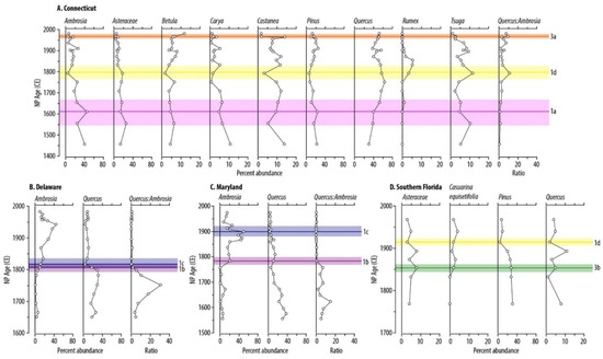
Figure 4.
Pollen stratigraphic diagrams plotted against the NP Bchron predicted ages to compare the age plus uncertainty of the pollen chronohorizons with the ages derived from other age markers at the depth where the pollen chronohorizon occurred for Connecticut (A), Delaware (B), Maryland (C), and Southern Florida (D). Lines indicate the pollen chronohorizons; shading indicates the uncertainty associated with each pollen chronohorizon. The chronohorizons are as follows: (3a) chestnut blight; (1d) beginning of the forestry industry; (1a) initial land clearance; (1c) lowest amount of forest cover; (1b) peak deforestation; and (3b) Casuarina introduction (Table 3).
Second, to identify the impact of pollen chronohorizons on the precision of age–depth models, we calculated the difference between the median 50% UI width of the NP and WP models. This was done for the individual pollen chronohorizons and for all pollen chronohorizons combined at each site, for a total of 24 models. Due to the accumulation model used by Bchron, pollen chronohorizons impacted the age–depth model not only at their identified depth, but also at surrounding depths. We focused our comparison between models on the area most influenced by the pollen chronohorizon: (a) the interval between the pollen chronohorizons and the nearest age marker, or (b) the interval 5 cm above or below the pollen chronohorizon of interest, whichever was larger. Comparisons including multiple pollen chronohorizons were analyzed from the age marker above the shallowest pollen chronohorizon to the age marker below the deepest pollen chronohorizon. We compared the measured widths of the 50% UIs of WP and NP swaths averaged over the defined interval to identify how pollen chronohorizons impacted the precision of age–depth models. We reported the differences between 50% UI swaths of WP and NP models in years and identified average differences of less than five years as representing “no change” (Figure 5, Table 4).
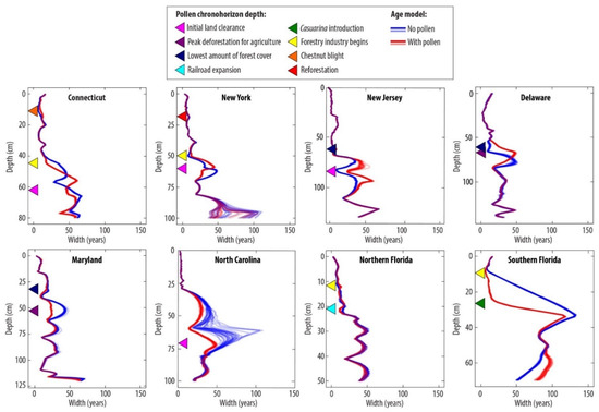
Figure 5.
Comparison of the difference in width of the 50% UI between the WP (all chronohorizon in red) and NP (blue) models over the interval from 1500 CE through the present (see also Figure A2). The red and blue lines are plotted transparently so that lighter areas represent widths that are predicted less frequently by Bchron, while darker areas represent widths that are predicted more frequently. The depth of the pollen chronohorizons is plotted using colored triangles which correspond to Figure 3.
Table 4.
Comparison of with pollen (WP) and no pollen (NP) age–depth models. Positive numbers in the columns titled “Average change of 50% UI width” represent a decrease in precision (widening) and negative numbers represent an increase in precision (narrowing). Average changes of <5 years are considered not to have changed. In the column titled “Average change in location of median”, positive numbers indicate that the addition of pollen caused the model to predict younger ages, while negative numbers indicate that including pollen caused the model to predict older ages for sediments in the depth range listed.
Third, to identify the impact of pollen chronohorizons on the Bchron-predicted age–depth relationship, we compared the position of the median age–depth model for WP and NP models, calculated based on the medians of the 31 replicate models. We determined the difference between the median of the NP and WP models, and compared them across the depth most influenced by the pollen chronohorizon(s) included in the model, as described above (Figure 6, Table 4). We found the average of these differences and report where the difference is in excess of five years as above.
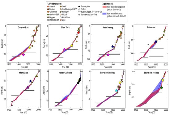
Figure 6.
Median Bchron age–depth models for all study sites with 50% UIs showing the WP model in red and the NP model in blue. These were calculated based on the median of all 31 replicates. UMV refers to lead pollution originating in the Upper Mississippi Valley.
4. Results
4.1. Connecticut
In Connecticut, we documented three pollen chronohorizons.
(1a) Initial land clearance associated with European settlement in 1700 ± 60 CE corresponds to a NP-predicted age range of 1515 to 1670 CE, indicating that the pollen chronohorizon is consistent with the ages predicted by the NP Bchron age–depth model (Figure 3, Table 3). The initial land clearance horizon increased the width of the 50% UI swath by 5 years and changed the position of the median age–depth model by +19 years (Figure 5, Table 4).
(1d) The beginning of the forestry industry in 1825 ± 25 CE is consistent with the NP-predicted age range of 1730 to 1840 CE (Figure 3, Table 3). The forestry industry signal narrowed the 50% UI swath by 7 years in the portion of the core surrounding the depth where it was documented (Figure 5, Table 4, Appendix D) and changed the position of the median age–depth model by +5 years (Table 4).
(3a) The chestnut blight chronohorizon in 1920 ± 10 CE is inconsistent with an NP-predicted age range of 1960 to 1970 CE in the NP age–depth model (Figure 3, Table 3). The chestnut blight chronohorizon did not change the width of the 50% UI swath (<5 years) (Figure 5, Table 4, Appendix D) or the position of the median Bchron age–depth model (<5 years) (Table 4).
4.2. New York
In New York, we documented three pollen chronohorizons.
(1a) Initial land clearance in 1680 ± 25 CE is consistent with the NP predicted age range of 1655 to 1800 CE (Table 3, Appendix C). Including this chronohorizon did not change the width of the 50% UI swath (<5 years); however, the position of the median age–depth model changed by −9 years (Figure 5, Table 4, Appendix D).
(1d) The beginning of the forestry industry in 1825 ± 25 CE has an NP-predicted age range of 1755 to 1835 CE, which is consistent with the other chronometers (Table 3, Appendix C). When this chronohorizon was included in the Bchron age–depth model, neither the width of the 50% UI swath nor the position of the median age–depth model position changed (both < 5 years) (Figure 5, Table 4, Appendix D)
(2a) Reforestation in 1960 ± 25 CE is associated with an NP-predicted age range of 1950 to 1965 CE, indicating that the pollen chronohorizon is consistent with other chronometers (Table 3, Appendix C). When the reforestation chronohorizon was included in the age–depth model, neither the width of the 50% UI swath nor the position of the median age–depth model changed (both < 5 years) (Figure 5, Table 4, Appendix D).
4.3. New Jersey
In New Jersey, we documented two pollen chronohorizons.
(1a) The timing of initial land clearance in New Jersey in 1710 ± 50 CE is consistent with the NP-predicted age range of 1570 to 1670 CE (Table 3, Appendix C). Including this chronohorizon in the age–depth model increased the width of the 50% UI swath by 14 years and changed the position of the median age–depth model by +8 years (Figure 5, Table 4, Appendix D).
(1c) The chronohorizon associated with the lowest amount of forest cover during a regional wood shortage that occurred in 1800 ± 20 CE is inconsistent with the NP-predicted age range of 1825 to 1850 CE (Table 3, Appendix C). When we included this chronohorizon in the Bchron age–depth model, neither the width of the 50% UI swath nor the position of the median age–depth model changed (< 5 years) (Figure 5, Table 4, Appendix D).
4.4. Delaware
In Delaware, we documented two pollen chronohorizons.
(1b) The chronohorizon associated with peak deforestation for agriculture in 1785 ± 15 CE is consistent with the NP-predicted age range of 1795 to 1815 CE (Figure 3, Table 3). The inclusion of this chronohorizon increased the width of the 50% UI swath by 11 years (Figure 5, Table 4, Appendix D) and changed the position of the median age–depth model by −7 years (Table 4).
(1c) The chronohorizon corresponding to the lowest amount of forest cover in 1800 ± 20 CE is consistent with an NP-predicted age range of 1800 to 1820 CE in the NP model (Figure 4, Table 3). When we included this chronohorizon in the Bchron age–depth model, the width of the 50% UI swath increased by 8 years and the position of the median age depth model changed by −6 years (Figure 5, Table 4, Appendix D).
4.5. Maryland
In Maryland, we documented two pollen chronohorizons.
(1b) The chronohorizon associated with peak deforestation for agriculture in 1785 ± 15 CE is consistent with an NP-predicted age range of 1740 to 1805 CE (Figure 4, Table 3). Including this chronohorizon decreased the width of the 50% UI swath by 5 years but did not change the position of the median age–depth model (<5 years) (Figure 5, Table 4, Appendix D).
(1c) The chronohorizon associated with the lowest amount of forest cover occurred in 1840 ± 20 CE and is inconsistent with the NP Bchron predicted age range of 1875 to 1915 CE (Figure 4, Table 3). When this chronohorizon was included in the age–depth model, neither the width of the 50% UI swath nor the position of the median age–depth model changed (both < 5 years) (Figure 5, Table 4, Appendix D).
4.6. North Carolina
We documented one pollen chronohorizon in North Carolina.
(1a) Initial land clearance in North Carolina occurred in 1720 ± 20 CE, which is consistent with the NP-predicted age range of 1610 to 1750 CE (Table 3, Appendix C). The inclusion of the initial land clearance chronohorizon decreased the width of the 50% UI swath by 20 years and changed the position of the median age–depth model by +20 years (Figure 5 and Figure 6, Table 4, Appendix D).
4.7. Northern Florida
We documented two pollen chronohorizons in northern Florida.
(1e) A chronohorizon associated with land clearance for railroad expansion in 1865 ± 15 CE is consistent with the NP-predicted age range of 1880 to 1905 CE (Table 3, Appendix C). When this chronohorizon was included in age–depth models, neither the width of the 50% UI swath nor the position of the median age–depth model changed (both < 5 years) (Figure 5, Table 4, Appendix D).
(1d) The chronohorizon associated with the beginning of the forestry industry in 1935 ± 10 CE is associated with an NP-predicted age range of 1940 to 1970 CE, which is consistent between the pollen chronohorizon and other age markers (Table 3, Appendix C). When this chronohorizon is included in the age–depth model, neither the width of the 50% UI swath nor the position of the median age–depth model changed (both < 5 years) (Figure 5, Table 4, Appendix D).
4.8. Southern Florida
We documented two pollen chronohorizons in southern Florida.
(3b) The chronohorizon associated with the introduction of Casuarina pollen in 1910 ± 15 CE is inconsistent with the NP-predicted age range of 1750 to 1885 CE (Figure 4, Table 3). When the Casuarina chronohorizon was included, it decreased the width of the 50% UI swath by 40 years (Figure 5, Table 4) and changed the position of the median age–depth model by +28 years (Table 4).
(1d) The chronohorizon associated with the beginning of the forestry industry resulting in the removal of Dade Pines from the Keys in 1935 ± 10 CE is consistent with the NP-predicted age range from 1895 to 1945 CE (Figure 4, Table 3). When we included this chronohorizon, it decreased the width of the 50% UI swath by 19 years but did not change the position of the median age–depth model (<5 years) (Figure 5, Table 4, Appendix D).
The inclusion of both chronohorizons greatly improved the Bchron age–depth model (Figure 6, Table 4): the width of the 50% UI swath decreased by 41 years. Additionally, the position of the median age–depth estimate changed by +23 years (Figure 5, Table 4, Appendix D).
5. Discussion
Pollen assemblages have been applied as chronometers throughout the Holocene [40], particularly during the last 500 years where the timing of events such as initial land clearance, industrial forestry, and recent importation or losses of taxa, help define anthropogenic alterations of the environment [25,40,44,79]. However, the application of pollen chronohorizons should proceed with caution in salt marsh environments, due to hyperlocality [40,63], sediment mixing [93,94,95], misinterpretation of pollen signals [74,75,96,97], and/or incorrect pollution and radiocarbon dates [98,99,100,101].
5.1. Validation of Pollen Chronohorizons
We validated the consistency of the pollen chronohorizons with other age markers by comparing the age ranges of pollen reference dates with Bchron age–depth models without pollen. While the majority of pollen chronohorizons were consistent with other age markers, four were inconsistent. Thirteen out of 17 pollen chronohorizons applied to cores were consistent with the chronology produced using the NP Bchron age–depth model (Table 3). Four pollen chronohorizons applied to cores were inconsistent with the NP chronology: the lowest amount of forest cover in Maryland; chestnut blight in Connecticut; the appearance of Casuarina in southern Florida; and the lowest amount of forest cover in New Jersey (Figure 4, Appendix C).
Pollen chronohorizons may be assigned an incorrect reference date due to hyperlocality (location-specific vegetation changes) and variations in regional signals [26,40,44,64,102]. The dispersal methods used by pollen can influence whether a signal is local or regional. Wind dispersal mechanisms are governed by atmospheric flow dynamics, landscape heterogeneity and climate, and differ among and within taxa because not all pollen grains are created equal [40,68,103,104]. It is well known that Pinus can be transported hundreds of kilometers [105], but models have shown that Ambrosia can also be transported hundreds of kilometers, suggesting that the Ambrosia pollen that we see in our cores may be local or regional [106,107]. In contrast, the pollen of Plantago and many other land-cover plants are transported only tens of meters. Therefore, when identifying a chronohorizon, the distance from the reference site should be considered when choosing which taxa to use [68,107]. Pollen transportation distances and production can also lead to specific, small localities having different timing or signals for chronohorizons, or hyperlocal effects [40,63]. Therefore, palynological changes may have occurred at different times at our study sites than at the reference location, resulting in hyperlocal effects [25,26,40].
Hyperlocality may also have affected the consistency of the lowest forest cover chronohorizon in Maryland. In our study, we applied a date of 1840 ± 20 for the lowest amount of forest cover, which is associated with peak Ambrosia [36]; however, this date was inconsistent with our NP-predicted age range of 1890–1910 at the depth where we observed this chronohorizon. In another study of Maryland pollen, the first peak of Ambrosia was found to correspond to peak lumber production between 1880 and 1920 [108]. This date is consistent with our NP-predicted date. Our date may be related to differences in the sampling locations because different parts of the Chesapeake Bay were deforested at different times [25].
In Connecticut, a large decline in chestnut pollen abundance occurs at 10 cm (Appendix C). Based on typical regional interpretations, this decline would be given a date of 1920 ± 10 CE [44,45], due to the appearance of chestnut blight in New York City in 1904 and subsequent spread throughout the northeastern U.S. within 50 years [109]; however, this date is inconsistent with our other chronometers. In Bridgeport and New Haven, Connecticut, proximal to our site, Japanese chestnut trees were a popular ornamental on estates, and their pollen, which is very similar to that of American chestnut, may have obscured the decline in native chestnut due to blight [110,111,112]. During the 1960s, the ornamental chestnut trees were cut down during suburbanization [113,114]. Therefore, it is possible that the hyperlocal signal associated with ornamental chestnuts and their removal obscured the chestnut blight signal, dating chestnut decline at 10 cm in Connecticut as approximately 1960, which is consistent with 137Cs peak, gasoline-related Pb minimum, Pb peak, and Hg peak (Table 1).
Pollen signals can also be misinterpreted due to the effects of sediment mixing and bioturbation. Salt marsh and mangrove environments are subject to mixing and bioturbation, which can cause smearing of signals used to construct chronologies [93,94]. In the case of bioturbation, plants or animals mix sediments through their growth, burrowing, or searching for food, resulting in signal peaks being smeared upward [94,95]. This is particularly true in mangrove environments, which are significantly impacted by the activities of root growth and crabs [115]. Salt marshes and mangrove environments are also subject to reworking due to tidal activity and storms [43,88,95]. For example, there is visual evidence of tidal and storm reworked sediments within the salt marsh stratigraphy of Connecticut from [53]. Sediment mixing may be responsible for the difficulties in selecting chronohorizons associated with initial land clearance and start of the forestry industry. The abundance of Ambrosia is high at the base of the Connecticut core, which is unexpected due to the paleobotanical history of the area, but may be due to mixing in the core [44,45]. Finally, mixing of the pollen signal may occur from the erosion of older pollen from one site and redeposition in another, causing an older chronohorizon to appear in a younger section of core than expected [116].
Pollen chronohorizons may be inconsistent with other chronometers due to misinterpretation in identifying pollen signals. Quantitative chronohorizons are based on specific numerical cutoffs [36], such as the first or last appearances of Casuarina or Castanea [44,45,65,66]. Therefore, quantitative chronohorizons should be more readily identifiable than qualitative chronohorizons that are based on unspecified increases or decreases in pollen relative abundance. For a qualitative increase, the percent abundance of the pollen species in question often varies before the increase, making choosing the correct depth more difficult (Appendix C) [74,75]. Additionally, there may be multiple interpretations for a given pollen chronohorizon. For example, the qualitative chronohorizon associated with initial land clearance in New Jersey could be interpreted at either 87.5 cm or 62.5 cm. We interpret the highest peak in Ambrosia at 87.5 cm as being associated with initial land clearance [36], whereas the pollen signals at 62.5 cm of increasing Ambrosia pollen, a sustained decrease in Quercus pollen, and the appearance of Plantago pollen are more consistent with the near-complete deforestation associated with lowest forest cover [36,37,76,78]. While both interpretations could be made, our interpretation is consistent with the other chronometers as the NP age range associated with 87.5 cm (1570 to 1670 CE) matches the reference date for initial land clearance in New Jersey of 1710 ± 50 years while the NP age range associated with 62.5 cm (1825 to 1870) does not.
A further issue that impacts both qualitative and quantitative chronohorizons is related to selecting the observed depth at which a pollen chronohorizon occurs—the event leading to the observation may have occurred between sampling depths. Depending on the sedimentation rate, a different sampling interval may impact the consistency of the pollen chronohorizons [96,97]. Sampling frequency can also affect the depth to which a chronohorizon is assigned [117,118]. Since pollen chronohorizons are assigned to depths where pollen is counted, a more frequent sampling interval will result in a more precise assignment of depth to a chronohorizon.
Finally, the other age markers may be based on erroneous dates, while the pollen date is accurate. Erroneous dating of other age markers could occur if a pollution marker or 137Cs peak was mobilized by groundwater [98,99,100,119]. For example, 137Cs bonds well with clay-sized sediment, but adheres less to organic particles, and therefore may be relatively mobile in organic salt marshes [99,120], particularly those high in humic acids, which keep 137Cs in its dissolved form [121,122,123]. However, in the published studies (Table 1), 20th century pollution markers and 137Cs peaks were used to reconstruct historical sea-level variability. The reconstructions were validated by instrumental tide gauge data, suggesting that these markers were in situ. Radiocarbon dates may also be erroneous through incorporation of either older carbon during sediment accumulation or younger carbon after deposition [101]. Contamination by younger carbon occurs as the result of root penetration or downward movement of humic acids [101,124]. However, all of our radiocarbon samples were prepared with careful screening procedures in an attempt to remove these contaminants.
5.2. Application of Pollen Chronohorizons to Improve the Age–Depth Model
Bchron’s Bayesian probability model, like all Bayesian models, has the property that increasing the data quantity (and quality) by incorporating pollen chronohorizons reduces the uncertainty in the resulting model [90,125]. Inclusion of a pollen chronohorizon in agreement with other age markers improves the confidence in the model [90,126] and allows the model to choose the most probable and perhaps accurate path [90,126]. For example, in North Carolina, the pollen chronohorizon associated with initial land clearance was consistent with the other age markers and was, therefore, able to help Bchron identify a different and more precise path by 20 years between the deepest pollution age marker and the shallowest radiocarbon date (Figure 6, Table 4).
Pollen chronohorizons also influence the precision of the age–depth models. The width of the 50% UI increased in six of the 24 models, decreased in seven models, and in 11 models had little or no change in precision (Table 4). Increases in precision ranged from five to 41 years. Several large increases (>10 years) in precision were evident with the addition of the following pollen chronohorizons: initial land clearance in North Carolina, the beginning of the forestry industry in southern Florida, the appearance of Casuarina in southern Florida, and all age markers combined in southern Florida (Figure 5). In each of these models, the pollen chronohorizons are located in a temporally restricted portion (the portion with few age markers) of the core between pollution markers and radiocarbon dates or near poorly constrained radiocarbon dates. The radiocarbon dates commonly have 2σ age ranges between ~30 to >300 years (Table 1 and Table 2). In this temporally restricted region, pollen chronohorizons are particularly important as they provide dated depths in a portion of the core that is otherwise difficult to reconstruct [6,38,39,40,127]. In the age–depth model from North Carolina, for example, the inclusion of the initial land clearance pollen chronohorizon between the youngest radiocarbon date and the oldest pollution age marker increased the precision by narrowing the 50% UI of the age–depth model by an average of 20 years (Figure 4 and Figure 5).
Pollen chronohorizons increased the 50% UI width (i.e., decreased precision) in six cases by 5 to 16 years (Figure 5, Table 4). Two of these models included at least one inconsistent chronometer (initial land clearance and combined age markers in New Jersey) (Table 4). We do not, however, advise discarding pollen chronohorizons that do not improve precision unless they can be quantitatively determined to be an outlier.
Additionally, pollen chronohorizons sometimes have conflicting results (i.e., consistent chronohorizons fail to improve model precision or inconsistent chronohorizons improve model precision). For example, the overlap between the peak deforestation chronohorizon uncertainty in Delaware and the NP age range for its corresponding depth is only six years, which may lead to it decreasing precision in the model (Table 3). In New York, the pollen chronohorizon associated with reforestation occurs around 1960 [73], a time where several other age markers are also present, such as dates associated with 137Cs onset and peak in 1954 and 1963, respectively, and a minimum in gasoline-related Pb isotopes in 1965 (Figure 6) [30,82]. Because there is sufficient time control in this section of core even without pollen included, Bchron is already able to produce narrow 50% UIs, and the inclusion of pollen chronohorizons cannot greatly improve upon the already precise model. Finally, an inconsistent pollen chronohorizon may improve the precision of the age–depth model when it occurs in a data poor area, such as the Casuarina introduction chronohorizon in southern Florida, suggesting a change in sedimentation rate that was not accounted for due to the sparsity of chronometers when pollen was excluded (Figure 5 and Figure 6).
5.3. Improving Pollen Chronohorizons
To further improve age–depth models, pollen chronohorizons could be developed or adapted. For example, a new pollen chronohorizon could be developed based on the increase in Iva pollen. At our Connecticut site, there is an increase in Iva pollen at 34 cm at which corresponds to an age of 1865 to 1879. A similar increase is seen in New Jersey at 36 cm to 37 cm (1900 to 1916) and New York at 16 cm to 17 cm (1939 to 1946). A possible explanation for the increase in Iva is ditching to drain salt marshes so that they could be farmed or as a method of mosquito control [63]. The ditching and draining decreased flooding and improved the marsh-upland edge habitat preferred by Iva [128]. Ditching of salt marshes began in the late 1800s through early 1900s in Connecticut [61,63], in 1907 in New Jersey [60,129], and in 1913 near New York City (Miller, 2001). Additional sources could be used to constrain the specific timing of historical increases in ditching and other land-use changes in tidal wetlands.
6. Conclusions
We have collected published and unpublished pollen and chronology data (e.g., radiocarbon, 137Cs, and pollution horizons) from coastal wetlands along the U.S. Atlantic Coast to determine if pollen chronohorizons are consistent with other chronometers and if including pollen chronohorizons improves the precision of age–depth models. We reviewed the vegetation histories and regional literature to identify eight unique pollen chronohorizons with a maximum of three chronohorizons per study region. The eight pollen chronohorizons were applied to 24 age–depth models for the eight study regions (17 models using individual chronohorizons and seven models with combined age markers).
We found that the ages assigned to 13 out of 17 applications of individual pollen chronohorizons were consistent when compared with dates derived by the NP Bchron chronology. In four applications, the pollen chronohorizons were inconsistent in Connecticut (Chestnut blight) and Maryland (lowest forest cover) due to hyperlocality of pollen chronohorizons, in Connecticut (land clearance) due to sediment mixing, and in New Jersey (land clearance) due to misinterpretation of the pollen signals, and/or incorrect pollution and radiocarbon dates. A possible solution to the inconsistency of pollen chronohorizons is to down-weigh in Bchron and other Bayesian age–depth models using outlier probabilities [130], which has been previously applied to erroneous radiocarbon dates [131,132].
We also assessed if the pollen chronohorizons improved the precision of the age depth models by comparing the median WP and NP 50% UIs. In seven out of the total of 24 models, inclusion of one or more pollen chronohorizons in the age–depth model improved the precision by up to 41 years. In six of 24 models, the WP model reduced the precision. Precision was most improved with the addition of pollen chronohorizons at sites with insufficient data, such as the land clearance pollen chronohorizon in North Carolina and the pollen chronohorizons observed in southern Florida, and where pollen chronohorizons were consistent with other age markers, such as the start of the forestry industry in Connecticut. Reductions in precision were often due to wide uncertainty ranges for pollen chronohorizons and inconsistency of pollen chronohorizons with other age markers, such as the initial land clearance chronohorizon in New Jersey. Overall, the inclusion of pollen chronohorizons in age–depth models pertaining to salt marsh and mangrove environments can be helpful in situations where other types of age markers are sparse or have large age uncertainties. Sedimentary environments which contain abundant pollen with a known vegetation history are excellent candidates for this approach, particularly if other dates are lacking, unavailable, or uncertain. Including one or more pollen chronohorizons in such cases improves the robustness of the age–depth model.
Author Contributions
M.A.C.: Conceptualization, Methodology, Software, Validation, Formal Analysis, Investigation, Writing—Original Draft, Writing—Review and Editing, Visualization, Project Administration. C.E.B.: Conceptualization, Methodology, Writing—Review and Editing. A.C.P.: Conceptualization, Methodology, Software, Validation, Writing—Review and Editing. T.A.S.: Investigation, Data Curation, Writing—Review and Editing, Visualization. N.S.K.: Investigation, Data Curation, Writing—Review and Editing. D.R.C.: Investigation, Writing—Review and Editing. A.G.-A.: Investigation, Data Curation, Writing—Review and Editing. J.C.: Investigation, Data Curation, Writing—Review and Editing. J.S.W.: Investigation, Data Curation, Writing—Review and Editing. J.P.D.: Investigation, Data Curation, Methodology, Writing—Review and Editing. T.R.H.: Methodology, Software, Writing—Review and Editing, Visualization. B.P.H.: Project Administration, Supervision, Funding Acquisition, Conceptualization, Writing—Review and Editing. All authors have read and agreed to the published version of the manuscript.
Funding
MC was funded by the National Science Foundation EAR 1624551. NSK, TS, and BPH were funded by the Ministry of Education Academic Research Fund MOE2018-T2-1-030 and MOE2019-T3-1-004, the National Research Foundation Singapore, and the Singapore Ministry of Education, under the Research Centres of Excellence initiative. This article is a contribution to International Geoscience Program (IGCP) Project 639, “Sea Level Change from Minutes to Millennia”. This work is Earth Observatory of Singapore contribution 349. AP wishes to acknowledge the funding Science Foundation Ireland Career Development Award (17/CDA/4695); an investigator award (16/IA/4520); a Marine Research Programme funded by the Irish Government, co-financed by the European Regional Development Fund (Grant-Aid Agreement No. PBA/CC/18/01); European Union’s Horizon 2020 research and innovation programme under grant agreement No 818144; and SFI Research Centre awards 16/RC/3872 and 12/RC/2289_P2.
Institutional Review Board Statement
Not applicable.
Informed Consent Statement
Not applicable.
Data Availability Statement
The data presented in this study are available in this paper. Data from published studies are available in the referenced papers.
Acknowledgments
MC wishes to acknowledge Andy Kemp for his support and advice throughout the process of studying pollen chronohorizons and Debra Willard for U.S. Geological Survey review of the manuscript. Any use of trade, product, or firm names is for descriptive purposes only and does not imply endorsement by the U.S. Government.
Conflicts of Interest
The authors declare no conflict of interest.
Appendix A
Table A1.
Chronological data for published sites. UMV refers to lead (Pb) pollution originating from the Upper Mississippi Valley. YBP = years before present.
Table A1.
Chronological data for published sites. UMV refers to lead (Pb) pollution originating from the Upper Mississippi Valley. YBP = years before present.
| Connecticut [48] | New York [51] | New Jersey [52] | ||||||||||
|---|---|---|---|---|---|---|---|---|---|---|---|---|
| Lab Code | Depth (cm) | Age (14C Years) | Calibrated Age Range (YBP) | Lab Code | Depth (cm) | Age (14C Years) | Calibrated Age Range (YBP) | Lab Code | Depth (cm) | Age (14C Years) | Calibrated Age Range (YBP) | |
| Radiocarbon | OS-88674 | 56 ± 2 | 175 ± 30 | 3–284 | OS-102551 | 60 ± 1 | 165 ± 25 | 6–280 | 14C10 | 76 ± 1 | 120 ± 30 | 18–265 |
| OS-86561 | 66 ± 2 | 345 ± 25 | 318–480 | OS-108259 | 70 ± 1 | 380 ± 30 | 325–500 | 14C12 | 82 ± 1 | 230 ± 25 | 1–305 | |
| OS-86562 | 78 ± 2 | 550 ± 30 | 523–633 | OS-108260 | 81 ± 1 | 285 ± 25 | 294–432 | 14C4 | 86 ± 1 | 250 ± 40 | 4–431 | |
| OS-89141 | 90 ± 2 | 835 ± 25 | 696–786 | OS-102552 | 95 ± 1 | 770 ± 30 | 672–733 | 14C11 | 94 ± 1 | 285 ± 30 | 289–447 | |
| OS-86567 | 111 ± 2 | 1080 ± 30 | 936–1053 | OS-115123 | 105 ± 1 | 695 ± 20 | 574–676 | 14C8 | 111 ± 1 | 400 ± 25 | 336–505 | |
| OS-86616 | 146 ± 2 | 1300 ± 25 | 1186–1284 | OS-109016 | 123 ± 1 | 1420 ± 30 | 1294–1369 | 14C5 | 122 ± 1 | 520 ± 40 | 508–29 | |
| OS-86560 | 156 ± 2 | 1490 ± 25 | 1323–1410 | OS-115122 | 127 ± 1 | 1120 ± 15 | 979–1056 | 14C1 | 135 ± 1 | 770 ± 30 | 672–733 | |
| OS-89764 | 158 ± 2 | 1490 ± 30 | 1317–1480 | OS-102598 | 137 ± 1 | 1180 ± 35 | 996–1213 | 14C2 | 145 ± 1 | 865 ± 25 | 720–890 | |
| OS-89059 | 165 ± 2 | 1570 ± 25 | 1406–1525 | OS-102553 | 155 ± 1 | 1560 ± 25 | 1396–1522 | 14C6 | 160 ± 1 | 960 ± 40 | 785–936 | |
| OS-88962 | 184 ± 2 | 1790 ± 25 | 1629–1807 | OS-102554 | 161 ± 1 | 1630 ± 35 | 1419–1605 | 14C3 | 171 ± 1 | 1100 ± 30 | 946–1061 | |
| 14C13 | 180 ± 1 | 1120 ± 25 | 969–1069 | |||||||||
| 14C7 | 194 ± 1 | 1190 ± 35 | 1008–1225 | |||||||||
| 14C9 | 208 ± 1 | 1350 ± 30 | 1193–1307 | |||||||||
| Depth (cm) | Age (year CE) | Age Marker | Depth (cm) | Age (year CE) | Age Marker | Depth (cm) | Age (year CE) | Age Marker | ||||
| Other Age Markers | 1 ± 4 | 1980 ± 5 | Gas Pb Peak | 5 ± 2 | 1980 ± 5 | Gas Pb Peak | 4.5 ± 4 | 1997 ± 5 | Ni Peak | |||
| 3 ± 4 | 1970 ± 5 | Hg Peak | 7 ± 2.5 | 1963 ± 1 | 137Cs Peak | 21 ± 4 | 1980 ± 5 | Gas Pb Peak | ||||
| 4 ± 4 | 1963 ± 1 | 137Cs Peak | 11 ± 2 | 1974 ± 5 | Pb Peak | 21 ± 4 | 1974 ± 5 | Pb Peak | ||||
| 9 ± 6 | 1974 ± 5 | Pb Peak | 11 ± 2 | 1970 ± 5 | V Peak | 36.5 ± 12 | 1969 ± 11 | Ni Onset | ||||
| 13 ± 6 | 1965 ± 5 | Zn Peak | 11 ± 1.5 | 1954 ± 2 | 137Cs Onset | 29 ± 4 | 1965 ± 5 | Gas Pb Min | ||||
| 19 ± 6 | 1935 ± 6 | Great Depression Pb Min | 13 ± 6 | 1970 ± 5 | Cu Peak | 17 ± 2 | 1963 ± 1 | 137Cs Peak | ||||
| 21 ± 4 | 1905 ± 5 | Hg Peak | 17 ± 6 | 1965 ± 5 | Gas Pb Min | 24.5 ± 4 | 1963 ± 7 | Cd Peak | ||||
| 22 ± 6 | 1880 ± 20 | UMV Decline | 21 ± 4 | 1937 ± 5 | Peak Incin. | 28.5 ± 4 | 1956 ± 13 | Zn Peak | ||||
| 31 ± 6 | 1900 ± 5 | Cu Onset | 27 ± 2 | 1933 ± 6 | Great Depression Pb Min | 29 ± 4 | 1948 ± 15 | Pb Min | ||||
| 33 ± 6 | 1925 ± 5 | Pb Peak | 33 ± 2 | 1900 ± 5 | Cu Onset | 33 ± 4 | 1925 ± 5 | Pb Peak | ||||
| 33 ± 4 | 1865 ± 10 | Hg Onset | 39 ± 2 | 1925 ± 5 | Pb Peak | 32.5 ± 4 | 1900 ± 10 | Cu Onset | ||||
| 37 ± 6 | 1858 ± 5 | UMV Peak | 41 ± 8 | 1857 ± 5 | UMV Peak | 44.5 ± 8 | 1890 ± 10 | Zn Onset | ||||
| 43 ± 6 | 1875 ± 5 | Pb Onset | 51 ± 2 | 1827 ± 5 | UMV Onset | 45 ± 4 | 1880 ± 5 | UMV Decline | ||||
| 43 ± 6 | 1827 ± 5 | UMV onset | 49 ± 4 | 1875 ± 5 | Pb Onset | |||||||
| 59 ± 4 | 1857 ± 5 | UMV Peak | ||||||||||
| 69 ± 4 | 1827 ± 5 | UMV Onset | ||||||||||
| North Carolina [42,53] | Northern Florida [27] | |||||||||||
| Sample Code | Depth (cm) | Age (14C Years) | Calibrated Age Range (YBP) | Lab Code | Depth (cm) | Age (14C Years) | Calibrated Age Range (YBP) | |||||
| Radiocarbon | HP14C1 | 60 ± 2 | 203 ± 11 | 0–286 | OS-99682 | 27 ± 1 | 185 ± 20 | 2–284 | ||||
| HP14C2 | 80 ± 2 | 338 ± 10 | 321–455 | OS-94713 | 33 ± 1 | 380 ± 35 | 322–501 | |||||
| RC1 | 87 ± 2 | 315 ± 25 | 309–457 | OS-96816 | 41 ± 1 | 515 ± 25 | 513–610 | |||||
| RC2 | 99 ± 2 | 535 ± 30 | 517–627 | OS-94715 | 51 ± 1 | 850 ± 30 | 699–884 | |||||
| RC3 | 114 ± 2 | 725 ± 25 | 658–692 | OS-96817 | 64 ± 1 | 1100 ± 25 | 956–1055 | |||||
| RC4 | 120 ± 2 | 755 ± 30 | 667–727 | OS-99683 | 74 ± 1 | 1400 ± 25 | 1289–1342 | |||||
| RC5 | 135 ± 2 | 900 ± 50 | 714–918 | OS-96497 | 82 ± 1 | 1660 ± 25 | 1529–1612 | |||||
| RC6 | 144 ± 2 | 910 ± 30 | 750–910 | OS-96495 | 91 ± 1 | 1830 ± 40 | 1640–1860 | |||||
| RC7 | 158 ± 2 | 1000 ± 25 | 812–957 | OS-94640 | 110 ± 1 | 2280 ± 30 | 2179–2345 | |||||
| RC8 | 168 ± 2 | 1080 ± 30 | 937–1053 | OS-96501 | 125 ± 1 | 2420 ± 25 | 2361–2673 | |||||
| RC9 | 189 ± 2 | 1190 ± 30 | 1017–1216 | |||||||||
| RC10 | 204 ± 2 | 1520 ± 40 | 1330–1518 | |||||||||
| RC11 | 217 ± 2 | 1600 ± 25 | 1417–1545 | |||||||||
| RC12 | 228 ± 2 | 1730 ± 35 | 1563–1711 | |||||||||
| RC13 | 248 ± 2 | 1920 ± 45 | 1742–1970 | |||||||||
| RC14 | 258 ± 2 | 2090 ± 35 | 1973–2143 | |||||||||
| RC15 | 268 ± 2 | 2120 ± 25 | 2012–2157 | |||||||||
| RC16 | 285 ± 2 | 2620 ± 45 | 2551–2833 | |||||||||
| RC17 | 299 ± 2 | 2420 ± 35 | 2360–2683 | |||||||||
| Depth (cm) | Age (year CE) | Age Marker | Depth (cm) | Age (year CE) | Age Marker | |||||||
| Other Age Markers | 18 ± 1 | 1996 ± 2 | Bomb Spike 14C | 3 ± 4 | 1998 ± 3 | Cu Peak | ||||||
| 19 ± 1 | 1989 ± 2 | Bomb Spike 14C | 5 ± 4 | 1980 ± 5 | Pb Gas Peak | |||||||
| 21 ± 1 | 1987 ± 2 | Bomb Spike 14C | 9 ± 4 | 1963 ± 1 | 137Cs Peak | |||||||
| 23 ± 1 | 1988 ± 1 | Bomb Spike 14C | 9 ± 4 | 1972 ± 6 | Cu Peak | |||||||
| 23 ± 4 | 1963 ± 1 | 137Cs Peak | 11 ± 4 | 1974 ± 5 | Pb Peak | |||||||
| 26 ± 1 | 1974 ± 1 | Bomb Spike 14C | 11 ± 4 | 1965 ± 5 | Pb Gas Min | |||||||
| 28 ± 1 | 1957 ± 1 | Bomb Spike 14C | 16 ± 6 | 1900 ± 10 | Coal Pb Peak | |||||||
| 29 ± 1 | 1958 ± 1 | Bomb Spike 14C | 17 ± 4 | 1935 ± 6 | Great Depression Pb Min | |||||||
| 17 ± 4 | 1900 ± 10 | Cu Onset | ||||||||||
| 19 ± 4 | 1925 ± 5 | Pb Peak | ||||||||||
| 23 ± 4 | 1875 ± 5 | Pb Onset | ||||||||||
| 23 ± 4 | 1870 ± 10 | Coal Pb Onset | ||||||||||
Appendix B
B.1. Southern Delaware
The southern Delaware site is located in the Great Marsh, northwest of Lewes, DE (38.78, −75.18). It is 20 km2 in area and is separated from the Delaware Bay by a sand barrier [133]. The tidal range is 1.4 m and tides are semi-diurnal (NOAA tide gauge, Station ID: 8557380). The tidal range has been influenced by anthropogenic activities, such as ditching and deforestation since the 1930s [37,134]. The southern Delaware site has a vertical zonation of plants: the low marsh is dominated by Spartina alterniflora tall form; the high marsh by Spartina alterniflora short form, Spartina patens, and Distichlis spicata; and the transition to freshwater upland by Phragmites australis, Iva frutescens, and Baccharis halimifolia. The climate at this site is warm temperate, and it has hot, humid summers [135]. The monthly average highs and lows range between 45 and −2 °C in January to 30 and 20 °C in July [136]. There is an average of 117 cm of precipitation at the southern Delaware site per year [136].
B.2. Maryland
The Maryland site is located in the Kirkpatrick salt marsh (38.87, −76.55). This salt marsh is located at the Smithsonian Environmental Research Center (SERC), near Mayo, Maryland and is on the northern Chesapeake Bay. It encompasses approximately 70 hectares of brackish marsh. The Maryland site is microtidal, with wind-influenced tides of less than 0.3 m. This site is dominated by Phragmites australis, Spartina alterniflora, and Distichlis spicata, with patches of Spartina patens. The wetland cored for the Maryland site is used for a variety of long-term environmental experiments by SERC [137]. The climate at the Maryland site is warm temperate [135]. The average monthly high and low temperatures at this site range between 7 and −2 °C in January to 32 and 22 °C in July [136]. At the Maryland site, 120 cm of precipitation per year on average [136].
B.3. Southern Florida
The southern Florida site is located on Swan Key in the Florida Keys (25.34, −80.25). This site is a microtidal mangrove swamp with a great diurnal range of 0.44 m (NOAA tide gauge, Station ID: 8723467). The mangrove swamp is dominated by three species of mangroves: Rhizophora mangle, Avicennia germinans, and Laguncularia racemosa. The climate at the southern Florida site is classified as a tropical savannah climate, with wet and dry periods throughout the year [59]. The average high is 28 °C and the average low is 21 °C with 145 cm of precipitation per year [136].
Appendix C

Figure A1.
Pollen stratigraphic diagrams for published data plotted against the NP Bchron predicted ages to compare the age plus uncertainty of the pollen chronohorizons with the ages derived from other age markers at the depth where the pollen chronohorizon occurred for New York (A), New Jersey (B), North Carolina (C), and Northern Florida (D). Colored lines indicate the pollen chronohorizons; colored shading indicates the uncertainty associated with each pollen chronohorizon. The colors refer to Figure 3. The chronohorizons are as follows: (2a) reforestation; (1d) beginning of the forestry industry; (1a) initial land clearance; (1c) lowest amount of forest cover; and (1e) railroad expansion (Table 3).
Appendix D

Figure A2.
Comparison of the difference in width of the 50% UI between the WP (red) and the NP (blue) models for each of the individual chronohorizon models over the interval from 1500 CE through the present. The red and blue lines are plotted transparently so that lighter areas represent widths that are predicted less frequently by Bchron, while darker areas represent widths that are predicted more frequently.
References
- Crowley, T.J. Causes of Climate Change Over the Past 1000 Years. Science 2000, 289, 270–277. [Google Scholar] [CrossRef] [PubMed]
- Mann, M.E.; Zhang, Z.; Rutherford, S.; Bradley, R.S.; Hughes, M.K.; Shindell, D.; Ammann, C.; Faluvegi, G.; Ni, F. Global Signatures and Dynamical Origins of the Little Ice Age and Medieval Climate Anomaly. Science 2009, 326, 1256–1260. [Google Scholar] [CrossRef] [PubMed]
- Reynolds, D.J.; Scourse, J.D.; Halloran, P.R.; Nederbragt, A.J.; Wanamaker, A.D.; Butler, P.G.; Richardson, C.A.; Heinemeier, J.; Eiriksson, J.; Knudsen, K.L.; et al. Annually resolved North Atlantic marine climate over the last millennium. Nat. Commun. 2016, 7, 13502. [Google Scholar] [CrossRef] [PubMed]
- Jones, M.C.; Bernhardt, C.E.; Krauss, K.W.; Noe, G.B. The impact of late Holocene land use change, climate variability, and sea level rise on carbon storage in tidal freshwater wetlands on the southeastern United States coastal plain. J. Geophys. Res. Biogeosci. 2017, 122, 3126–3141. [Google Scholar] [CrossRef]
- Stager, J.C.; Wiltse, B.; Hubeny, J.B.; Yankowsky, E.; Nardelli, D.; Primack, R. Climate variability and cultural eutrophication at Walden Pond (Massachusetts, USA) during the last 1800 years. PLoS ONE 2018, 13, e0191755. [Google Scholar] [CrossRef]
- Gorham, E.; Brush, G.S.; Graumlich, L.J.; Rosenzweig, M.L.; Johnson, A.H. The value of paleoecology as an aid to monitoring ecosystems and landscapes, chiefly with reference to North America. Environ. Rev. 2001, 9, 99–126. [Google Scholar] [CrossRef]
- Schurer, A.P.; Mann, M.E.; Hawkins, E.; Tett, S.F.B.; Hegerl, G.C. Importance of the pre-industrial baseline for likelihood of exceeding Paris goals. Nat. Clim. Chang. 2017, 7, 563–568. [Google Scholar] [CrossRef]
- Reiners, P.W.; Carlson, R.W.; Renne, P.R.; Cooper, K.M.; Granger, D.E.; McLean, N.M.; Schoene, B. Geochronology and Thermochronology; John Wiley & Sons: Hoboken, NJ, USA, 2017. [Google Scholar]
- Noller, J.; Sowers, J.M.; Coleman, S.M.; Pierce, K. Introduction to Quaternary Geochronology; American Geophysical Union: Washington, DC, USA, 2000. [Google Scholar]
- Libby, W.F.; Anderson, E.C.; Arnold, J.R. Age Determination by Radiocarbon Content: World-Wide Assay of Natural Radiocarbon. Science 1949, 109, 227–228. [Google Scholar] [CrossRef]
- Stuiver, M.; Reimer, P.J.; Bard, E.; Beck, J.W.; Burr, G.S.; Hughen, K.A.; Kromer, B.; McCormac, G.; Van Der Plicht, J.; Spurk, M. INTCAL98 radiocarbon age calibration, 24,000–0 cal BP. Radiocarbon 1998, 40, 1041–1083. [Google Scholar] [CrossRef]
- Reimer, P.J.; Bard, E.; Bayliss, A.; Beck, J.W.; Blackwell, P.G.; Bronk Ramsey, C.; Buck, C.E.; Cheng, H.; Edwards, R.L.; Friedrich, M.; et al. INTCAL13 and MARINE13 Radiocarbon Age Calibration Curves 0–50,000 Years Cal BP. Radiocarbon 2013, 55, 1869–1887. [Google Scholar] [CrossRef]
- Hua, Q. Radiocarbon: A chronological tool for the recent past. Quat. Geol. 2009, 4, 378–390. [Google Scholar] [CrossRef]
- Stuiver, M. Radiocarbon timescale tested against magnetic and other dating methods. Nature 1978, 273, 271–274. [Google Scholar] [CrossRef]
- Keeling, C.D. The Suess effect: 13Carbon-14Carbon interrelations. Environ. Int. 1979, 2, 229–230. [Google Scholar] [CrossRef]
- Tans, P.P.; Mook, W.G. Design, construction, and calibration of a high accuracy Carbon-14 counting system. Radiocarbon 1978, 21, 22–40. [Google Scholar] [CrossRef]
- Reimer, P.J.; Reimer, R.W. Radiocarbon Dating: Calibration. In Encyclopedia of Quaternary Science; Elais, S.A., Ed.; Elsevier: Oxford, UK, 2007; pp. 2941–2949. [Google Scholar]
- Hua, Q.; Barbetti, M.; Rakowski, A.Z. Atmospheric radiocarbon for the period 1950–2010. Radiocarbon 2013, 55, 2059–2072. [Google Scholar] [CrossRef]
- Goldberg, E.D. Geochronology with 210Pb Radioactive Dating; International Atomic Energy Agency: Vienna, Austria, 1963; Volume 121, p. 130. [Google Scholar]
- Appleby, P.G.; Oldfield, F. Application of 210-Pb to sedimentation studies. In Uranium-Series Disequilibrium: Applications to Earth, Marine, & Environmental Studies; Ivanovich, M., Harmon, R.S., Eds.; Oxford University Press: Oxford, UK, 1992; pp. 731–778. [Google Scholar]
- Robbins, J.A. Geochemical and geophysical applications of radioactive lead. In Biogeochemistry of Lead in the Environment; Elsevier Scientific: Oxford, UK, 1978; pp. 285–293. [Google Scholar]
- Cutshall, N.H.; Larsen, I.L.; Olsen, C.R. Direct analysis of 210Pb in sediment samples: Self-absorption corrections. Nucl. Instrum. Methods Phys. Res. 1983, 206, 309–312. [Google Scholar] [CrossRef]
- He, Q.; Walling, D.E. Rates of Overbank Sedimentation on the Floodplains of British Lowland Rivers Documented Using Fallout 137Cs. Geogr. Ann. Ser. A Phys. Geogr. 1996, 78, 223–234. [Google Scholar] [CrossRef]
- Walling, D.E.; He, Q. Models for converting 137-Cs measurements to estimates of soil redistribution rates on cultivated and uncultivated soils (including software for model implementation). In Report to IAEA; University of Exeter: Exeter, UK, 1997. [Google Scholar]
- Brush, G.S. Rates and patterns of estuarine sediment accumulation. Limnol. Oceanogr. 1989, 34, 1235–1246. [Google Scholar] [CrossRef]
- Cooper, S.R.; McGlothlin, S.K.; Madritch, M.; Jones, D.L. Paleoecological Evidence of Human Impacts on the Neuse and Pamlico Estuaries of North Carolina, USA. Estuaries 2004, 27, 617–633. [Google Scholar] [CrossRef]
- Kemp, A.C.; Bernhardt, C.E.; Horton, B.P.; Kopp, R.E.; Vane, C.H.; Pertier, W.R.; Hawkes, A.D.; Donnelly, J.P.; Parnell, A.C.; Cahill, N. Late Holocene sea- and land-level change on the U.S. southeastern Atlantic Coast. Mar. Geol. 2014, 357, 90–100. [Google Scholar] [CrossRef]
- MacKenzie, A.B.; Hardie, S.M.L.; Farmer, J.G.; Eades, L.J.; Pulford, I.D. Analytical and sampling constraints in 210Pb dating. Sci. Total Environ. 2011, 409, 1298–1304. [Google Scholar] [CrossRef] [PubMed]
- Barsanti, M.; Garcia-Tenorio, R.; Schirone, A.; Rozmaric, M.; Ruiz-Fernández, A.C.; Sanchez-Cabeza, J.A.; Delbono, I.; Conte, F.; Godoy, J.D.O.; Heijnis, H.; et al. Challenges and limitations of the 210Pb sediment dating method: Results from an IAEA modelling interlaboratory comparison exercise. Quat. Geochronol. 2020, 59, 101093. [Google Scholar] [CrossRef]
- Varekamp, J.C.; Kreulen, B.; Buchholtz ten Brink, M.R.; Mecrey, E.L. Mercury contamination chronologies from Connecticut wetlands and Long Island Sound sediments. Environ. Geol. 2003, 4, 468–482. [Google Scholar] [CrossRef]
- Schottler, S.P.; Engstrom, D.R. A chronological assessment of Lake Okeechobee (Florida) sediments using multiple dating markers. J. Paleolimnol. 2006, 36, 19–36. [Google Scholar] [CrossRef]
- Metcalfe, S.; Derwent, D. Atmospheric Pollution and Environmental Change; Routledge: Abingdon, UK, 2014. [Google Scholar]
- Katz, A.; Kaplan, I.R. Heavy metal behavior in coastal sediments of southern California: A critical review and synthesis. Mar. Chem. 1981, 10, 261–299. [Google Scholar] [CrossRef]
- Sanchez-Cabeza, J.A.; Druffel, E.R. Environmental records of anthropogenic impacts on coastal ecosystems: An introduction. Mar. Pollut. Bull. 2009, 59, 87–90. [Google Scholar] [CrossRef][Green Version]
- Kemp, A.C.; Sommerfield, C.S.; Vane, C.H.; Horton, B.P.; Chenery, S.R.; Anisfeld, S.; Nikitina, D. Use of lead isotopes for developing chronologies in recent salt-marsh sediments. Quat. Geochronol. 2012, 12, 40–49. [Google Scholar] [CrossRef]
- Brush, G.S. Patterns of recent sediment accumulation in Chesapeake Bay (Virginia-Maryland, USA) tributaries. Chem. Geol. 1984, 44, 227–242. [Google Scholar] [CrossRef]
- Matlack, G.R. Four Centuries of Forest Clearance and Regeneration in the Hinterland of a Large City. J. Biogeogr. 1997, 24, 281–295. [Google Scholar] [CrossRef]
- Roe, H.M.; Van de Plassche, O. Modern pollen distribution in a Connecticut saltmarsh: Implications for studies of sea-level change. Quat. Sci. Rev. 2005, 24, 2030–2049. [Google Scholar] [CrossRef]
- Hilgartner, W.B.; Brush, G.S. Prehistoric habitat stability and post-settlement habitat change in a Chesapeake Bay freshwater tidal wetland, USA. Holocene 2006, 16, 479–494. [Google Scholar] [CrossRef]
- Bernhardt, C.E.; Willard, D.A. Pollen and spores of terrestrial plants. In Handbook of Sea-Level Research; Shennan, I., Long, A.J., Horton, B.P., Eds.; Wiley: Hoboken, NJ, USA, 2015; pp. 218–232. [Google Scholar]
- Pederson, D.C.; Peteet, D.M.; Kurdyla, D.; Guilderson, T. Medieval Warming, Little Ice Age, and European impact on the environment during the last millennium in the lower Hudson Valley, New York, USA. Quat. Res. 2005, 63, 238–249. [Google Scholar] [CrossRef]
- Kemp, A.C.; Kegel, J.J.; Culver, S.J.; Barber, D.C.; Mallinson, D.J.; Leorri, E.; Bernhardt, C.E.; Bernhardt, C.E.; Cahill, N.; Riggs, S.R.; et al. Extended late Holocene relative sea-level histories for North Carolina, USA. Quat. Sci. Rev. 2017, 160, 13–30. [Google Scholar] [CrossRef]
- Donnelly, J.P.; Roll, S.; Wengren, M.; Butler, J.; Lederer, R.; Webb III, T. Sedimentary evidence of intense hurricane strikes from New Jersey. Geology 2001, 29, 615–618. [Google Scholar] [CrossRef]
- Brugam, R.B. Pollen indicators of land-use change in southern Connecticut. Quat. Res. 1978, 9, 349–362. [Google Scholar] [CrossRef]
- Clark, J.S.; Patterson, W.A. Pollen, Pb-210, and opaque spherules; an integrated approach to dating and sedimentation in the intertidal environment. J. Sediment. Res. 1984, 54, 1251–1265. [Google Scholar]
- Mudie, P.J.; Byrne, R. Pollen evidence for historic sedimentation rates in California salt-marshes. Estuar. Coast. Mar. Sci. 1980, 10, 305–316. [Google Scholar] [CrossRef]
- Bernabo, J.C.; Webb, T. Changing patterns in the Holocene pollen record of northeastern North America: A mapped summary. Quat. Res. 1977, 8, 64–96. [Google Scholar] [CrossRef]
- Barbier, E.D.; Hacker, S.D.; Kennedy, C.; Koch, E.W.; Stier, A.C.; Silliman, B.R. The value of estuarine and coastal ecosystem services. Ecol. Monogr. 2011, 81, 169–193. [Google Scholar] [CrossRef]
- Gedan, K.B.; Silliman, B.R.; Bertness, M.D. Centuries of Human-Driven Change in Salt-Marsh Ecosystems. Annu. Rev. Mar. Sci. 2009, 1, 117–144. [Google Scholar] [CrossRef]
- Craft, C.; Clough, J.; Ehman, J.; Joye, S.; Park, R.; Pennings, S.; Guo, H.; Machmuller, M. Forecasting the Effects of Accelerated Sea-Level Rise on Tidal Marsh Ecosystem Services. Front. Ecol. Environ. 2008, 7, 73–78. [Google Scholar] [CrossRef]
- Deegan, L.A.; Johnson, D.S.; Warren, R.S.; Peterson, B.J.; Fleeger, J.W.; Fagherazzi, S.; Wollheim, W.M. Coastal eutrophication as a driver of salt marsh loss. Nature 2012, 490, 388–392. [Google Scholar] [CrossRef] [PubMed]
- Horton, B.P.; Shennan, I.; Bradley, S.L.; Cahill, N.; Kirwan, M.; Kopp, R.E.; Shaw, T.A. Predicting marsh vulnerability to sea-level rise using Holocene relative sea-level data. Nat. Commun. 2018, 9, 1–7. [Google Scholar] [CrossRef] [PubMed]
- Kemp, A.C.; Hawkes, A.D.; Donnelly, J.P.; Vane, C.H.; Horton, B.P.; Hill, T.D.; Anisfeld, S.C.; Parnell, A.C.; Cahill, N. Relative sea-level change in Connecticut (USA) during the last 2200 yrs. Earth Planet. Sci. Lett. 2015, 428, 217–229. [Google Scholar] [CrossRef]
- Parnell, A.C. Bchron: Radiocarbon Dating, Age-Depth Modelling, Relative Sea Level Rate Estimation, and Non-Parametric Phase Modelling. Available online: https://rdrr.io/cran/Bchron/ (accessed on 15 June 2018).
- USDA Forest Service. USFS Forest Inventory and Analysis (FIA) Program; Geospatial Technology and Applications Center (GTAC) National Forest Type Dataset. Available online: https://data.fs.usda.gov/geodata/rastergateway/forest_type/ (accessed on 12 February 2019).
- Kemp, A.C.; Hill, T.D.; Vane, C.H.; Cahill, N.; Orton, P.M.; Talke, S.A.; Parnell, A.C.; Sanborn, K.; Hartig, E.L. Relative sea-level trends in New York City during the past 1500 years. Holocene 2017, 27, 1169–1186. [Google Scholar] [CrossRef]
- Kemp, A.C.; Horton, B.P.; Vane, C.H.; Bernhardt, C.E.; Corbett, D.R.; Engelhart, S.E.; Anisfeld, S.C.; Parnell, A.C.; Cahill, N. Sea-level change during the last 2500 years in New Jersey, USA. Quat. Sci. Rev. 2013, 81, 90–104. [Google Scholar] [CrossRef]
- Kemp, A.C.; Buzas, M.A.; Horton, B.P.; Culver, S.J. Influence of patchiness on modern salt-marsh foraminifera used in sea-level studies (North Carolina, USA). J. Foraminifer. Res. 2011, 41, 114–123. [Google Scholar] [CrossRef]
- Peel, M.C.; Finlayson, B.L.; McMahon, T.A. Updated world map of the Köppen-Geiger climate classification. Hydrol. Earth Syst. Sci. 2007, 11, 1633–1644. [Google Scholar] [CrossRef]
- Burger, J.; Shisler, J. Nest site selection and competitive interactions of herring and laughing gulls in New Jersey. Auk 1978, 95, 252–266. [Google Scholar]
- Rozsa, R. Human impacts on tidal wetlands: History and regulations. Vol. Bulletin No. 34. In Tidal Marshes of Long Island Sound: Ecology, History and Restoration; Dreyer, G.D., Niering, W.A., Eds.; The Connecticut Arboretum Press: New London, CT, USA, 1995; pp. 42–50. [Google Scholar]
- Miller, J.R. The Control of Mosquito-Borne Diseases in New York City. J. Urban Health Bull. N. Y. Acad. Med. 2001, 78, 359–366. [Google Scholar] [CrossRef]
- Bromberg, K.D.; Bertness, M.D. Reconstructing New England Salt-marsh Losses Using Historical Maps. Estuaries 2005, 28, 823–832. [Google Scholar] [CrossRef]
- McAndrews, J.H. Human disturbance of North American forests and grasslands: The fossil pollen record. In Handbook of Vegetation Science; Huntley, B., Webb, T., III, Eds.; Kluwer Academic Publishing: Dordrecht, The Netherlands, 1988; Volume 7. [Google Scholar]
- Alexander, T.R.; Crook, A.G. Recent vegetational changes in southern Florida. Environments of Southern Florida: Present and Past. Memoir 1974, 2, 61–72. [Google Scholar]
- Morton, J.F. The Australian pine or Beefwood (Casuarina equisetifolia), and invasive “weed” tree in Florida. Proc. Fla. Hortic. Soc. 1980, 93, 87–95. [Google Scholar]
- De Vleescheuwer, F.; Chambers, F.M.; Swindles, G.T. Coring and sub-sampling of peatlands for paleoenvironmental research. Mires Peat 2010, 7, 1–10. [Google Scholar]
- Faegri, K.; J Iverson, J. Textbook on Pollen Analysis, 4th ed.; Hafner: New York, NY, USA, 1989. [Google Scholar]
- Foster, D.R.; Zebryk, T.; Schoonmaker, P.; Lezberg, A. Post-settlement history of human land-use and vegetation dynamics of a Tsuga canadensis (hemlock) woodlot in central New England. J. Ecol. 1992, 80, 773–786. [Google Scholar] [CrossRef]
- Nevel, R.L., Jr.; Stochia, E.L.; Wahl, T. New York Timber Industries—A Periodic Assessment of Timber Output, Resource Bulletin NE-73; United States Department of Agriculture, Forest Service, Northeast Forest Experimental Station: Upper Darby, PA, USA, 1982.
- Burrows, E.G.; Wallace, M. Gotham: A History of New York City to 1898; Oxford University Press: Oxford, UK, 2000. [Google Scholar]
- Russell, E.W.B. Vegetational Change in Northern New Jersey from Precolonization to the Present: A Palynological Interpretation. Bull. Torrey Bot. Club 1980, 107, 432–446. [Google Scholar] [CrossRef]
- Fain, J.J.; Volk, T.A.; Fahey, T.J. Fifty Years of Change in an Upland Forest in South-Central New York: General Patterns. Bull. Torrey Bot. Club 1994, 121, 130–139. [Google Scholar] [CrossRef]
- Wacker, P.O. Land and People: A Cultural Geography of Preindustrial New Jersey Origins and Settlement Patterns; Rutgers University Press: Newark, NJ, USA, 1975; Volume 1. [Google Scholar]
- Wacker, P.O.; Clemens, P.G.E. Land Use in Early New Jersey; A Historical Geography; Rutgers University Press: Newark, NJ, USA, 1994. [Google Scholar]
- Bones, J.T. The Timber Industries of New Jersey and Delaware, Resource Bulletin NE-28; United States Department of Agriculture, Forest Service, Northeastern Forest Experimental Station: Upper Darby, PA, USA, 1973.
- Jones, C.F. A landscape of energy abundance: Anthracite. Coal Canals and the Roots of American Fossil Fuel Dependence, 1820–1860. Environ. Hist. 2010, 15, 449–484. [Google Scholar] [CrossRef]
- Johannes, J.H. Yesterday’s Reflections: Nassau County, Florida: A Pictorial History. Nassau Co. Florida: T.O. Richardson. 1976. Available online: http://www.wnhsfl.org/nassau-county-history.html (accessed on 12 February 2019).
- Wingard, G.L.; Hudley, J.W.; Holmes, C.W.; Willard, D.A.; Marot, M. Synthesis of Age Data and Chronology for Florida Bay and Biscayne Bay Cores Collected for Ecosystem History of South Florida’s Estuaries Project; No. 2007-1203; US Geological Survey: Reston, VA, USA, 2007.
- Marshall, F.E.; Bernhardt, C.E.; Wingard, G.L. Estimating Late 19th Century Hydrology in the Greater Everglades Ecosystem: An Integration of Paleoecologic Data and Models. Front. Environ. Sci. 2020, 8, 3. [Google Scholar] [CrossRef]
- Niu, M.; Heaton, T.J.; Blackwell, P.G.; Buck, C.E. The Bayesian approach to radiocarbon calibration curve estimation: The IntCal13, Marine13, and SHCal13 methodologies. Radiocarbon 2013, 55, 1905–1922. [Google Scholar] [CrossRef]
- UNSCEAR. Sources and Effects of Ionizing Radiation; Report to the General Assembly; United Nations: New York, NY, USA, 2000. [Google Scholar]
- He, Q.; Walling, D.E. The distribution of fallout 137-Cs and 210-Pb in undisturbed and cultivated soils. Appl. Radioact. Isot. 1997, 48, 677–690. [Google Scholar] [CrossRef]
- Marcantonio, F.; Zimmerman, A.; Xu, Y.; Canuel, E. A Pb isotope record of mid-Atlantic U.S. atmospheric Pb emissions in Chesapeake Bay sediments. Mar. Chem. 2002, 77, 123–132. [Google Scholar] [CrossRef]
- Lima, A.L.; Bergquist, B.A.; Boyle, E.A.; Reuer, M.K.; Dudas, F.O.; Reddy, C.M.; Eglinton, T.I. High-resolution historical records from Pettaquamscutt River basin sediments: 2. Pb isotopes reveal a potential new stratigraphic marker. Geochim. Cosmochim. Acta 2005, 69, 1813–1824. [Google Scholar] [CrossRef]
- Hurst, R.W. Lead isotopes as age-sensitive genetic markers in hydrocarbons. 3. Leaded gasoline, 1923–1990 (ALAS model). Environ. Geosci. 2002, 9, 43–50. [Google Scholar] [CrossRef]
- Bricker-Urso, S.; Nixon, S.W.; Cochran, J.K.; Hirschberg, D.J.; Hunt, C. 1989. Accretion rates and sediment accumulation in Rhode Island salt-marshes. Estuaries 1989, 12, 300–317. [Google Scholar] [CrossRef]
- Donnelly, J.P.; Bryant, S.S.; Butler, J.; Dowling, J.; Fan, L.; Hausmann, N.; Newby, P.; Shuman, B.; Stern, J.; Westover, K.; et al. A 700-year sedimentary record of intense hurricane landfalls in southern New England. Geol. Soc. Am. Bull. 2001, 113, 714–727. [Google Scholar] [CrossRef]
- Haslett, J.; Parnell, A. A simple monotone process with application to radiocarbon-dated depth chronologies. J. R. Stat. Soc. 2008, 3, 399–418. [Google Scholar] [CrossRef]
- Parnell, A.C.; Haslett, J.; Allen, J.R.M.; Buck, C.E.; Huntley, B. A flexible approach to assessing synchroneity of past events using Bayesian reconstructions of sedimentation history. Quat. Sci. Rev. 2008, 27, 1872–1885. [Google Scholar] [CrossRef]
- Scott, E.M.; Cook, G.; Naysmith, P. The fifth international radiocarbon intercomparison (VIRI): An assessment of laboratory performance in stage 3. Radiocarbon 2010, 53, 859–865. [Google Scholar] [CrossRef]
- David, H.A.; Nagaraja, H.N. Order Statistics; Wiley Series in Probability and Statistics: New York, NY, USA, 2003. [Google Scholar]
- Sharma, P.; Gardner, L.R.; Moore, W.S.; Bollinger, M.S. Sedimentation and bioturbation in a salt-marsh as revealed by 210Pb, 137Cs, and 7Be studies. Limnol. Oceanogr. 1987, 32, 313–326. [Google Scholar] [CrossRef]
- Vernberg, F.J. Salt-marsh processes: A review. Environ. Toxicol. Chem. 1993, 12, 2167–2195. [Google Scholar] [CrossRef]
- Leorri, E.; Martin, R.E.; Horton, B.P. Field experiments on bioturbation in salt-marshes (Bombay Hook National Wildlife Refuge, Smyrna, DE, USA: Implications for sea-level studies. J. Quat. Sci. 2009, 24, 139–149. [Google Scholar] [CrossRef]
- Jacobson, G.L.; Bradshaw, R.H.W. The Selection of Sites for Paleovegetational Studies. Quat. Res. 1981, 16, 80–96. [Google Scholar] [CrossRef]
- MacDonald, G.M. Fossil pollen analysis and the reconstruction of plant invasions. In Advances in Ecological Research; Academic Press: Cambridge, MA, USA, 1993; Volume 24, pp. 67–110. [Google Scholar]
- Dubinski, B.J.; Simpson, R.L.; Good, R.E. The retention of heavy metals in sewage sludge applied to a freshwater tidal wetland. Estuaries 1986, 9, 102–111. [Google Scholar] [CrossRef]
- Bryant, C.L.; Farmer, J.G.; MacKenzie, A.B.; Baily-Watt, A.E.; Kirika, A. Distribution and behaviour of radiocaesium in Scottish freshwater loch sediments. Environ. Geochem. Health 1993, 15, 153–161. [Google Scholar] [CrossRef] [PubMed]
- Amos, K.J.; Croke, J.C.; Timmers, H.; Owens, P.N.; Thompson, C. The application of caesium-137 measurements to investigate floodplain deposition in a large semi-arid catchment in Queensland, Australia: A low-fallout environment. Earth Surf. Process. Landf. 2009, 34, 515–529. [Google Scholar] [CrossRef]
- Kemp, A.C.; Nelson, A.R.; Horton, B.P. Radiocarbon Dating of Plant Macrofossils from Tidal-Marsh Sediment. In Methods in Geomorphology, in Treatise on Geomorphology; Switzer, A.D., Kennedy, D.M., Eds.; Academic Press: San Diego, CA, USA, 2013; Volume 14, pp. 370–388. [Google Scholar]
- Marshall, W. Chronohorizons: Indirect and unique event dating methods for sea-level reconstructions. In Handbook for Sea-Level Research; Shennan, I., Long, A.J., Horton, B.P., Eds.; Wiley: Hoboken, NJ, USA, 2015; pp. 373–385. [Google Scholar]
- Schueler, S.; Schlünzen, K.H. Modeling of oak pollen dispersal on the landscape level with a mesoscale atmospheric model. Environ. Model. Assess. 2006, 11, 179–194. [Google Scholar] [CrossRef]
- Trondman, A.K.; Gaillard, M.J.; Mazier, F.; Sugita, S.; Fyfe, R.; Nielsen, A.B.; Twiddle, C.; Barratt, P.; Birks, H.J.B.; Bjune, A.E.; et al. Pollen-based quantitative reconstructions of Holocene regional vegetation cover (plant-functional types and land-cover types) in Europe suitable for climate modelling. Glob. Chang. Biol. 2015, 21, 676–697. [Google Scholar] [CrossRef]
- Traverse, A. Paleopalynology, 2nd ed.; Springer Science & Business Media: Berlin/Heidelberg, Germany, 2007; Volume 28. [Google Scholar]
- McLauchlan, K.K.; Barnes, C.S.; Craine, J.M. Interannual variability of pollen productivity and transport in mid-North America from 1997 to 2009. Aerobiologia 2011, 27, 181–189. [Google Scholar] [CrossRef]
- Zink, K.; Vogel, H.; Vogel, B.; Magyar, D.; Kottmeier, C. Modeling the dispersion of Ambrosia artemisiifolia L. pollen with the model system COSMO-ART. Int. J. Biometeorol. 2012, 56, 669–680. [Google Scholar] [CrossRef]
- Willard, D.A.; Cronin, T.M.; Verardo, S. Late-Holocene climate and ecosystem history from Chesapeake Bay sediment cores, USA. Holocene 2003, 13, 201–214. [Google Scholar] [CrossRef]
- Anderson, T.W. The chestnut pollen decline as a time horizon in lake sediments in eastern North America. Can. J. Earth Sci. 1974, 11, 678–685. [Google Scholar] [CrossRef]
- Anagnostakis, S.L.; Hillman, B. Evolution of the Chestnut Tree and Its Blight. Arnoldia 1992, 52, 2–10. [Google Scholar]
- Anagnostakis, S.L. Chestnuts and the Introduction of Chestnut Blight. The Agricultural Connecticut Experimental Station. Available online: https://www.ct.gov/CAES/cwp/view.asp?a=2815&q=376754 (accessed on 10 October 2018).
- Anagnostakis, S.L. American Chestnuts in the 21st Century. Arnoldia 2009, 66, 23–31. [Google Scholar]
- Nicolaides, B.; Wiese, A. Suburbanization in the United States after 1945; Oxford Research Encyclopedias: American History; Oxford University Press: Oxford, UK, 2017; Available online: http://americanhistory.oxfordre.com/view/10.1093/acrefore/9780199329175.001.0001/acrefore-9780199329175-e-64 (accessed on 10 October 2018).
- Anagnostakis, S.L. (Department of Plant Pathology and Ecology, The Connecticut Agricultural Experiment Station, New Haven, CT, USA). Personal communication, 2018.
- Ellison, J.C. Modeling of oak pollen dispersal on the landscape level with a mesoscale atmospheric model. Palaeogeogr. Palaeoclimatol. Palaeoecol. 1989, 74, 327–341. [Google Scholar] [CrossRef]
- Neulieb, T.; Levac, E.; Southon, J.; Lewis, M.; Pendea, I.F.; Chmura, G.L. Potential pitfalls of pollen dating. Radiocarbon 2013, 55, 1142–1155. [Google Scholar] [CrossRef]
- Turner, J.; Peglar, S.M. Temporally-precise studies of vegetation history. In Vegetation History; Springer: Dordrecht, The Netherlands, 1988; pp. 753–777. [Google Scholar]
- Bennington, J.B.; Rutherford, S.D. Precision and reliability in paleocommunity comparisons based on cluster-confidence intervals; how to get more statistical bang for your sampling buck. Palaios 1999, 14, 506–515. [Google Scholar] [CrossRef]
- Hovenac, C. Reconstructing the Erosional History of 19th-Century Earthen Fortifications along the Coastline of the Chesapeake Bay, Maryland, USA. Master’s Thesis, University of Delaware, Newark, DE, USA, 2015. [Google Scholar]
- Torgensen, T.; Longmore, M. 137Cs diffusion in the highly organic sediment of -Hidden Lake, Fraser Island, Queensland. Mar. Freshw. Res. 1984, 35, 537–548. [Google Scholar] [CrossRef]
- Farmer, J.G. The perturbation of historical pollution records in aquatic sediments. Environ. Geochem. Health 1991, 13, 76–83. [Google Scholar] [CrossRef]
- Abril, J.M. Constraints on the use of 137Cs as a time-marker to support CRS and SIT chronologies. Environ. Pollut. 2004, 129, 31–37. [Google Scholar] [CrossRef]
- Campbell, C.A.; Paul, E.A.; Rennie, D.A.; McCallum, R.J. Mid-infrared spectroscopy as a method of characterizing changes in soil organic matter. Soil Sci. Soc. Am. Proc. 1967, 77, 1591–1600. [Google Scholar]
- Thompson, J.; Dyer, F.M.; Croudace, I.W. Records of radionuclide deposition in two salt marshes in the United Kingdom with contrasting redox and accumulation conditions. Geochim. Cosmochim. Acta 2002, 66, 1011–1023. [Google Scholar] [CrossRef]
- Blaauw, M.; Christen, J.A.; Bennett, K.D.; Reimer, P.J. Double the dates and go for Bayes—Impacts of model choice, dating density and quality on chronologies. Quat. Sci. Rev. 2018, 188, 58–66. [Google Scholar] [CrossRef]
- Telford, R.J.; Heegaard, E.; Birks, H.J.B. All age–depth models are wrong: But how badly? Quat. Sci. Rev. 2004, 23, 1–5. [Google Scholar] [CrossRef]
- Brush, G.S.; Martin, E.A.; Defries, R.S.; Rice, C.A. Comparisons of 210Pb and Pollen Methods for Determining Rates of Estuarine Sediment Accumulation. Quat. Res. 1982, 18, 196–217. [Google Scholar] [CrossRef]
- Bertness, M.D.; Wikler, K.; Chatkupt, T. Flood tolerance and the distribution of Iva frutescens across New England salt-marshes. Oecologia 1992, 91, 171–178. [Google Scholar] [CrossRef]
- Smith, J.B. The New Jersey Salt-Marsh and Its Improvement; New Jersey Agricultural Environmental Station: New Brunswick, NJ, USA, 1907. [Google Scholar]
- Hamilton, W.D.; Kenney, J. Multiple Bayesian modelling approaches to a suite of radiocarbon dates from ovens excavated at Ysgol yr Hendre, Caernarfon, North Wales. Quat. Geol. 2014, 25, 72–82. [Google Scholar] [CrossRef]
- Bronk Ramsey, C. Bayesian analysis of radiocarbon dates. Radiocarbon 2009, 51, 337–360. [Google Scholar] [CrossRef]
- Blaauw, M.; Christen, J.A. Radiocarbon Peat Chronologies and Environmental Change. J. R. Stat. Soc. Ser. C (Appl. Stat.) 2005, 54, 805–816. [Google Scholar] [CrossRef]
- Stedman, S.M. Sedimentology and Stratigraphy of the Great Marsh, Lewes, Delaware. Ph.D. Thesis, University of Delaware, Newark, DE, USA, 1990. [Google Scholar]
- Wolfe, R.J. Effects of open marsh water management on selected tidal marsh resources: A review. J. Am. Mosq. Control Assoc. 1996, 12, 701–712. [Google Scholar]
- Kottek, M.; Grieser, J.; Beck, C.; Rudolf, B.; Rubel, F. World map of the Köppen-Geiger climate classification updated. Meteorol. Z. 2006, 15, 259–263. [Google Scholar] [CrossRef]
- Weather Service. US Climate Data. Available online: https://www.usclimatedata.com/ (accessed on 15 June 2018).
- Smithsonian Environmental Research Center. Available online: https://serc.si.edu/ (accessed on 18 November 2019).
Publisher’s Note: MDPI stays neutral with regard to jurisdictional claims in published maps and institutional affiliations. |
© 2021 by the authors. Licensee MDPI, Basel, Switzerland. This article is an open access article distributed under the terms and conditions of the Creative Commons Attribution (CC BY) license (http://creativecommons.org/licenses/by/4.0/).