New Zealand River Hydrology under Late 21st Century Climate Change


Abstract
1. Introduction
2. Materials and Methods
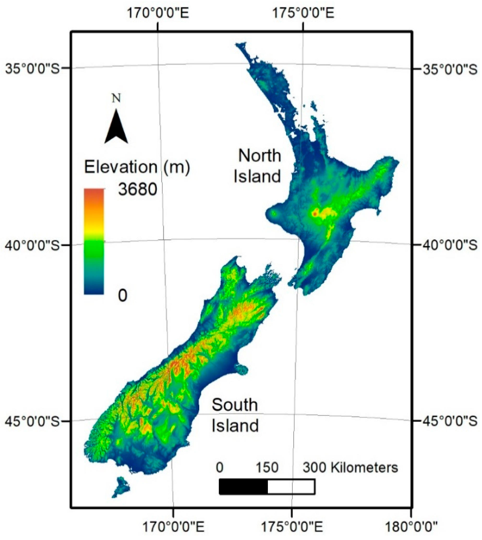
2.1. Study Region
2.2. Climate Data
2.3. Hydrological Modelling
2.4. Validation
2.5. Climate Change Impact Analysis
3. Results
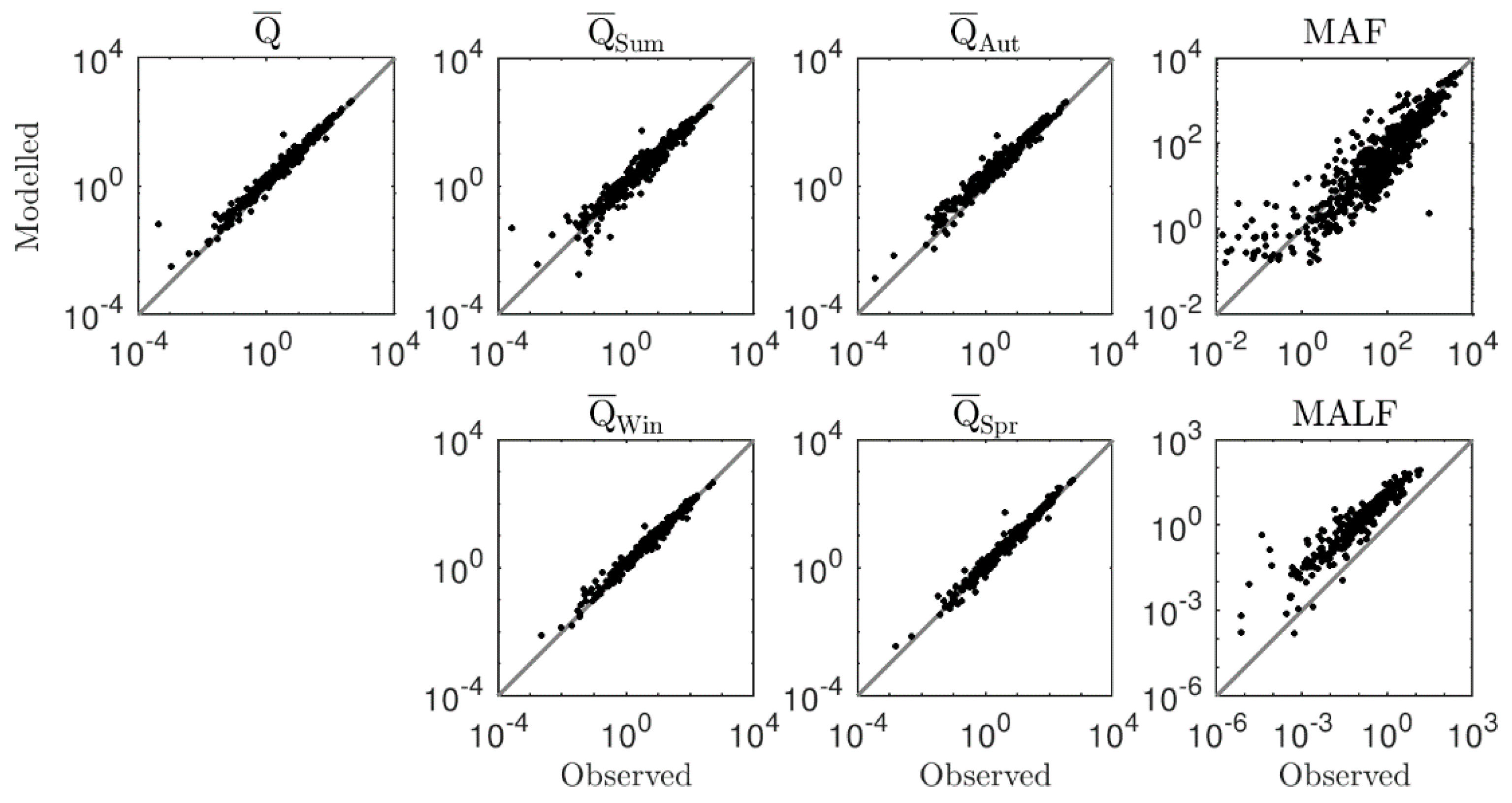
3.1. Validation
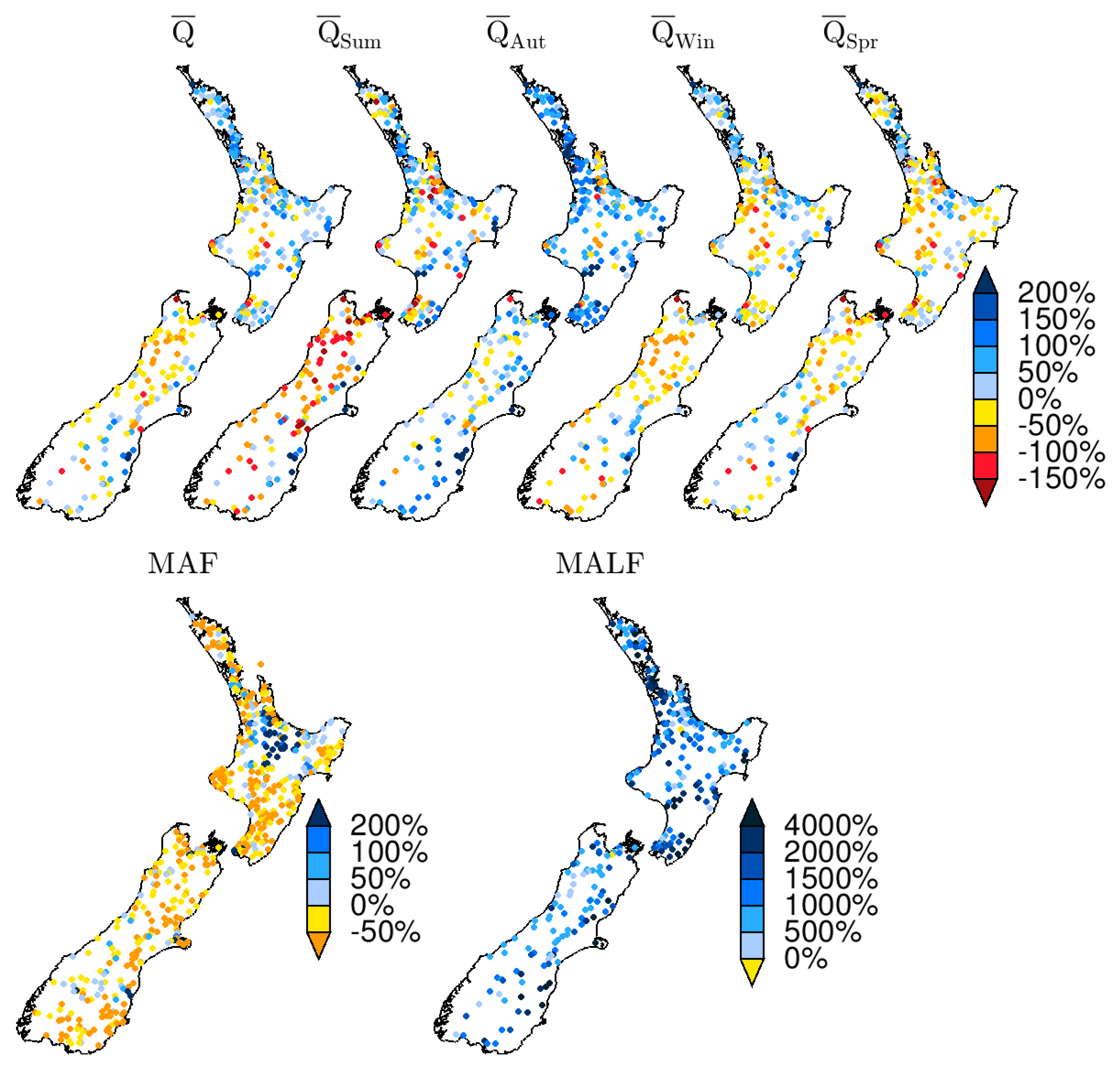
3.2. Changes in Mean Annual and Seasonal Flows
3.3. Changes in High and Low Flow Extremes
4. Discussion
4.1. Interpreting Hydrological Changes
4.2. Uncertainties and Limitations
4.3. National Coverage
5. Conclusions
Funding
Acknowledgments
Conflicts of Interest
References
- IPCC. Climate Change 2014: Impacts, Adaptation, and Vulnerability. Part A: Global and Sectoral Aspects. Contribution of Working Group II to the Fifth Assessment Report of the Intergovernmental Panel on Climate Change; Cambridge Univseristy Press: Cambridge, UK; New York, NY, USA, 2014; p. 1132. [Google Scholar]
- Bloschl, G.; Hall, J.; Parajka, J.; Perdigao, R.A.P.; Merz, B.; Arheimer, B.; Aronica, G.T.; Bilibashi, A.; Bonacci, O.; Borga, M.; et al. Changing climate shifts timing of European floods. Science 2017, 357, 588–590. [Google Scholar] [CrossRef] [PubMed]
- Donat, M.G.; Lowry, A.L.; Alexander, L.V.; O’Gorman, P.A.; Maher, N. More extreme precipitation in the world’s dry and wet regions. Nat. Clim. Chang. 2016, 6, 508–513. [Google Scholar] [CrossRef]
- Donnelly, C.; Greuell, W.; Andersson, J.; Gerten, D.; Pisacane, G.; Roudier, P.; Ludwig, F. Impacts of climate change on European hydrology at 1.5, 2 and 3 degrees mean global warming above preindustrial level. Clim. Chang. 2017, 143, 13–26. [Google Scholar] [CrossRef]
- Arnell, N.W.; Gosling, S.N. The impacts of climate change on river flood risk at the global scale. Clim. Chang. 2016, 134, 387–401. [Google Scholar] [CrossRef]
- Dai, A.G. Increasing drought under global warming in observations and models. Nat. Clim. Chang. 2013, 3, 52–58. [Google Scholar] [CrossRef]
- Hay, L.E.; Markstrom, S.L.; Ward-Garrison, C. Watershed-Scale Response to Climate Change through the Twenty-First Century for Selected Basins across the United States. Earth Interact. 2011, 15. [Google Scholar] [CrossRef]
- Lobanova, A.; Liersch, S.; Nunes, J.P.; Didovets, I.; Stagl, J.; Huang, S.; Koch, H.; Lopez, M.D.R.; Maule, C.F.; Hattermann, F. Hydrological impacts of moderate and high-end climate change across European river basins. J. Hydrol. Reg. Stud. 2018, 18, 15–30. [Google Scholar] [CrossRef]
- Distefano, T.; Kelly, S. Are we in deep water? Water scarcity and its limits to economic growth. Ecol. Econ. 2017, 142, 130–147. [Google Scholar] [CrossRef]
- Wrona, F.J.; Johansson, M.; Culp, J.M.; Jenkins, A.; Mard, J.; Myers-Smith, I.H.; Prowse, T.D.; Vincent, W.F.; Wookey, P.A. Transitions in Arctic ecosystems: Ecological implications of a changing hydrological regime. J. Geophys. Res. Biogeosci. 2016, 121, 650–674. [Google Scholar] [CrossRef]
- Alfieri, L.; Feyen, L.; Di Baldassarre, G. Increasing flood risk under climate change: A pan-European assessment of the benefits of four adaptation strategies. Clim. Chang. 2016, 136, 507–521. [Google Scholar] [CrossRef]
- Iglesias, A.; Garrote, L. Adaptation strategies for agricultural water management under climate change in Europe. Agric. Water Manag. 2015, 155, 113–124. [Google Scholar] [CrossRef]
- Langsdale, S. Communication of climate change uncertainty to stakeholders using the scenario approach. J. Contemp. Water Res. Educ. 2008, 140, 24–29. [Google Scholar] [CrossRef]
- Hakala, K.; Addor, N.; Teutschbein, C.; Vis, M.J.P.; Dakhlaoui, H.; Seibert, J. Hydrological modelling of climate change impacts. In Encyclopedia of Water: Science, Technology, and Society; Maurice, P., Ed.; WIley: Hoboken, NJ, USA, 2020; pp. 1–20. [Google Scholar]
- Van Vuuren, D.P.; Edmonds, J.; Kainuma, M.; Riahi, K.; Thomson, A.; Hibbard, K.; Hurtt, G.C.; Kram, T.; Krey, V.; Lamarque, J.F.; et al. The representative concentration pathways: An overview. Clim. Chang. 2011, 109, 5–31. [Google Scholar] [CrossRef]
- Clark, M.P.; Wilby, R.L.; Gutmann, E.D.; Vano, J.A.; Gangopadhyay, S.; Wood, A.W.; Fowler, H.J.; Prudhomme, C.; Arnold, J.R.; Brekke, L.D. Characterizing Uncertainty of the Hydrologic Impacts of Climate Change. Curr. Clim. Chang. Rep. 2016, 2, 55–64. [Google Scholar] [CrossRef]
- Wilby, R.L.; Dessai, S. Robust adaptation to climate change. Weather 2010, 65, 180–185. [Google Scholar] [CrossRef]
- McMillan, H.K.; Booker, D.J.; Cattoen, C. Validation of a national hydrological model. J. Hydrol. 2016, 541, 800–815. [Google Scholar] [CrossRef]
- Lee, S.; Kim, S.U. Quantification of Hydrological Responses Due to Climate Change and Human Activities over Various Time Scales in South Korea. Water 2017, 9, 34. [Google Scholar] [CrossRef]
- Roudier, P.; Ducharne, A.; Feyen, L. Climate change impacts on runoff in West Africa: A review. Hydrol. Earth Syst. Sci. 2014, 18, 2789–2801. [Google Scholar] [CrossRef]
- Leng, G.Y.; Huang, M.Y.; Voisin, N.; Zhang, X.S.; Asrar, G.R.; Leung, L.R. Emergence of new hydrologic regimes of surface water resources in the conterminous United States under future warming. Environ. Res. Lett. 2016, 11. [Google Scholar] [CrossRef]
- Mullan, A.B.; Stuart, S.J.; Hadfield, M.G.; Smith, M.J. Report on the Review of NIWA’s ‘Seven-Station’ Temperature Series; NIWA: Wellington, New Zealand, 2010; p. 175. [Google Scholar]
- Ministry for the Environment. Climate Change Predictions for New Zealand: Atmospheric Projections Based on Simulations Undertaken for the IPCC 5th Assessment, 2nd ed.; Ministry for the Environment: Wellington, New Zealand, 2018; p. 131.
- Caloiero, T. Analysis of rainfall trend in New Zealand. Environ. Earth Sci. 2015, 73, 6297–6310. [Google Scholar] [CrossRef]
- Collins, D. Physical changes to New Zealand’s freshwater ecosystems under climate change. In Proceedings of the Freshwater Conservation under a Changing Climate, Wellington, New Zealand, 10–11 December 2013; pp. 9–12. [Google Scholar]
- Collins, D.; Montgomery, K.; Zammit, C. Hydrological Projections for New Zealand Rivers under Climate Change; NIWA: Christchurch, New Zealand, 2018; p. 107. [Google Scholar]
- Collins, D.; Zammit, C. Climate Change Impacts on Agricultural Water Resources and Flooding; NIWA: Christchurch, New Zealand, 2016; p. 71. [Google Scholar]
- Robb, C.; Bright, J. Values and uses of water. In Freshwater of New Zealand; Hardin, J., Mosley, P., Pearson, C., Sorrell, B., Eds.; New Zealand Hydrological Society and New Zealand Limnological Society: Christchurch, New Zealand, 2004; pp. 42.1–42.13. [Google Scholar]
- Ministry for the Environment. National Policy Statement for Freshwater Management 2014; Ministry for the Environment: Wellington, New Zealand, 2017; p. 47.
- Resource Management Act. 1991. Available online: http://www.legislation.govt.nz/act/public/1991/0069/latest/DLM230265.html (accessed on 16 May 2020).
- Salinger, J.; Gray, W.; Mullan, B.; Wratt, D. Atmospheric circulation and precipitation. In Freshwaters of New Zealand; Harding, J., Mosley, P., Pearson, C., Sorrell, B., Eds.; New Zealand Hydrological Society and New Zealand Limnological Society: Christchurch, New Zealand, 2004; pp. 2.1–2.18. [Google Scholar]
- Pettinga, J. Rock formation and earth-building processes. In The Physical Environment: A New Zealand Perspective; Sturman, A., Spronken-Smith, R., Eds.; Oxford University Press: Melbourne, Australia, 2001. [Google Scholar]
- Newsome, P.F.J.; Wilde, R.H.; Willoughby, E.J. Land Resource Information System Spatial Data Layers; Landcare Research NZ Ltd.: Palmerston North, New Zealand, 2000. [Google Scholar]
- Macara, G.R. The Climate and Weather of New Zealand; NIWA: Wellington, Australia, 2018; p. 50. [Google Scholar]
- Owens, I.; Fitzharris, B. Seasonal snow and water. In Freshwaters of New Zealand; Harding, J., Mosley, P., Pearson, C., Sorrell, B., Eds.; New Zealand Hydrological Society and New Zealand Limnological Society: Christchurch, New Zealand, 2004; pp. 5.1–5.12. [Google Scholar]
- Ummenhofer, C.C.; Sen Gupta, A.; England, M.H. Causes of Late Twentieth-Century Trends in New Zealand Precipitation. J. Clim. 2009, 22, 3–19. [Google Scholar] [CrossRef]
- Toebes, C. The water balance of New Zealand. J. Hydrol. 1972, 11, 139–172. [Google Scholar]
- Woods, R.; Hendrikx, J.; Henderson, R.; Tait, A. Estimating mean flow of New Zealand rivers. J. Hydrol. 2006, 45, 95–110. [Google Scholar]
- Collins, D.; Zammit, C.; Willsman, A.; Henderson, R. Surface Water Components of New Zealand’s National Water Accounts, 1995–2014; NIWA: Christchurch, New Zealand, 2015; p. 18. [Google Scholar]
- Kerr, T. The contribution of snowmelt to the rivers of the South Island, New Zealand. J. Hydrol. 2013, 52, 61–82. [Google Scholar]
- Duncan, M.; Woods, R. Flow regimes. In Freshwaters of New Zealand; Harding, J., Mosley, P., Pearson, C., Sorrell, B., Eds.; New Zealand Hydrological Society and New Zealand Limnological Society: Christchurch, New Zealand, 2004; pp. 7.1–7.14. [Google Scholar]
- Pearson, C.; Henderson, R.D. Floods and low flows. In Freshwaters of New Zealand; Harding, J., Mosley, P., Pearson, C., Sorrell, B., Eds.; New Zealand Hydrological Society and New Zealand Limnological Society: Christchurch, New Zealand, 2004; pp. 10.1–10.16. [Google Scholar]
- Griffiths, G.A.; McKerchar, A.I. Estimation of mean annual flood in New Zealand. J. Hydrol. 2012, 51, 111–120. [Google Scholar]
- IPCC. Climate Change 2013: The Physical Science Basis. Contribution of Working Group I to the Fifth Assessment Report of the Intergovernmental Panel on Climate Change; Cambridge University Press: Cambridge, UK; New York, NY, USA, 2013; p. 1535. [Google Scholar]
- UNFCCC. Adoption of the Paris Agreement. FCCC/CP/2015/L.9/Rev1. 2015. Available online: https://unfccc.int/resource/docs/2015/cop21/eng/l09r01.pdf (accessed on 18 June 2020).
- Anagnostopoulou, C.; Tolika, K.; Mahera, P.; Kutiel, H.; Flocas, H.A. Performance of the general circulation HadAM3P model in simulating circulation types over the Mediterranean region. Int. J. Climatol. 2008, 28, 185–203. [Google Scholar] [CrossRef]
- Jones, P.D.; Lister, D.H.; Osborn, T.J.; Harpham, C.; Salmon, M.; Morice, C.P. Hemispheric and large-scale land-surface air temperature variations: An extensive revision and an update to 2010. J. Geophys. Res. Atmos. 2012, 117. [Google Scholar] [CrossRef]
- Ackerley, D.; Dean, S.; Sood, A.; Mullan, A.B. Regional climate modeling in New Zealand: Comparison to gridded and satellite observations. Weather Clim. 2012, 32, 3–22. [Google Scholar] [CrossRef]
- Clark, M.P.; Rupp, D.E.; Woods, R.A.; Zheng, X.; Ibbitt, R.P.; Slater, A.G.; Schmidt, J.; Uddstrom, M.J. Hydrological data assimilation with the ensemble Kalman filter: Use of streamflow observations to update states in a distributed hydrological model. Adv. Water Resour. 2008, 31, 1309–1324. [Google Scholar] [CrossRef]
- Snelder, T.H.; Biggs, B.J.F. Multiscale River Environment Classification for water resources management. J. Am. Water Resour. Assoc. 2002, 38, 1225–1239. [Google Scholar] [CrossRef]
- Booker, D.J.; Woods, R.A. Comparing and combining physically-based and empirically-based approaches for estimating the hydrology of ungauged catchments. J. Hydrol. 2014, 508, 227–239. [Google Scholar] [CrossRef]
- Krysanova, V.; Donnelly, C.; Gelfan, A.; Gerten, D.; Arheimer, B.; Hattermann, F.; Kundzewicz, Z.W. How the performance of hydrological models relates to credibility of projections under climate change. Hydrol. Sci. J. 2018, 63, 696–720. [Google Scholar] [CrossRef]
- Decremer, D.; Chung, C.E.; Ekman, A.M.L.; Brandefelt, J. Which significance test performs the best in climate simulations? Tellus Ser. A Dyn. Meteorol. Oceanogr. 2014, 66. [Google Scholar] [CrossRef]
- Poyck, S.; Hendrikx, J.; McMillan, H.; Hreinsson, E.O.; Woods, R. Combined snow and streamflow modelling to estimate impacts of climate change on water resources in the Clutha River, New Zealand. J. Hydrol. 2011, 50, 293–312. [Google Scholar]
- Jobst, A.M.; Kingston, D.G.; Cullen, N.J.; Schmid, J. Intercomparison of different uncertainty sources in hydrological climate change projections for an alpine catchment (upper Clutha River, New Zealand). Hydrol. Earth Syst. Sci. 2018, 22, 3125–3142. [Google Scholar] [CrossRef]
- Byun, K.; Chiu, C.M.; Hamlet, A.F. Effects of 21st century climate change on seasonal flow regimes and hydrologic extremes over the Midwest and Great Lakes region of the US. Sci. Total Environ. 2019, 650, 1261–1277. [Google Scholar] [CrossRef]
- Gobiet, A.; Kotlarski, S.; Beniston, M.; Heinrich, G.; Rajczak, J.; Stoffel, M. 21st century climate change in the European Alps-A review. Sci. Total Environ. 2014, 493, 1138–1151. [Google Scholar] [CrossRef]
- Berghuijs, W.R.; Woods, R.A.; Hrachowitz, M. A precipitation shift from snow towards rain leads to a decrease in streamflow. Nat. Clim. Chang. 2014, 4, 583–586. [Google Scholar] [CrossRef]
- Hagemann, S.; Chen, C.; Clark, D.B.; Folwell, S.; Gosling, S.N.; Haddeland, I.; Hanasaki, N.; Heinke, J.; Ludwig, F.; Voss, F.; et al. Climate change impact on available water resources obtained using multiple global climate and hydrology models. Earth Syst. Dyn. 2013, 4, 129–144. [Google Scholar] [CrossRef]
- Vetter, T.; Reinhardt, J.; Florke, M.; van Griensven, A.; Hattermann, F.; Huang, S.C.; Koch, H.; Pechlivanidis, I.G.; Plotner, S.; Seidou, O.; et al. Evaluation of sources of uncertainty in projected hydrological changes under climate change in 12 large-scale river basins. Clim. Chang. 2017, 141, 419–433. [Google Scholar] [CrossRef]
- Giuntoli, I.; Vidal, J.P.; Prudhomme, C.; Hannah, D.M. Future hydrological extremes: The uncertainty from multiple global climate and global hydrological models. Earth Syst. Dyn. 2015, 6, 267–285. [Google Scholar] [CrossRef]
- Schewe, J.; Heinke, J.; Gerten, D.; Haddeland, I.; Arnell, N.W.; Clark, D.B.; Dankers, R.; Eisner, S.; Fekete, B.M.; Colon-Gonzalez, F.J.; et al. Multimodel assessment of water scarcity under climate change. Proc. Natl. Acad. Sci. USA 2014, 111, 3245–3250. [Google Scholar] [CrossRef] [PubMed]
- Williams, J.; Morgenstern, O.; Varma, V.; Behrens, E.; Hayek, W.; Oliver, H.; Dean, S.; Mullan, B.; Frame, D. Development of the New Zealand Earth System Model: NZESM. Weather Clim. 2016, 36, 25–44. [Google Scholar] [CrossRef]
- Her, Y.; Yoo, S.H.; Cho, J.; Hwang, S.; Jeong, J.; Seong, C. Uncertainty in hydrological analysis of climate change: Multi-parameter vs. multi-GCM ensemble predictions. Sci. Rep. 2019, 9. [Google Scholar] [CrossRef]
- Zhu, X.P.; Zhang, A.R.; Wu, P.L.; Qi, W.; Fu, G.T.; Yue, G.T.; Liu, X.Q. Uncertainty Impacts of Climate Change and Downscaling Methods on Future Runoff Projections in the Biliu River Basin. Water 2019, 11, 2130. [Google Scholar] [CrossRef]
- Andreasson, J.; Bergstrom, S.; Carlsson, B.; Graham, L.P. The effect of downscaling techniques on assessing water resources impacts from climate change scenarios. In Proceedings of the Water Resources Systems—Water Availability and Global Change, Symposium HS02a of the 23rd General Assembly of the IUGG, Sapporo, Japan, 7–11 July 2003; pp. 160–164. [Google Scholar]
- Chen, J.; Brissette, F.P.; Chaumont, D.; Braun, M. Performance and uncertainty evaluation of empirical downscaling methods in quantifying the climate change impacts on hydrology over two North American river basins. J. Hydrol. 2013, 479, 200–214. [Google Scholar] [CrossRef]
- Iizumi, T.; Takikawa, H.; Hirabayashi, Y.; Hanasaki, N.; Nishimori, M. Contributions of different bias-correction methods and reference meteorological forcing data sets to uncertainty in projected temperature and precipitation extremes. J. Geophys. Res. Atmos. 2017, 122, 7800–7819. [Google Scholar] [CrossRef]
- Mendoza, P.A.; Clark, M.P.; Mizukami, N.; Newman, A.J.; Barlage, M.; Gutmann, E.D.; Rasmussen, R.M.; Rajagopalan, B.; Brekke, L.D.; Arnold, J.R. Effects of Hydrologic Model Choice and Calibration on the Portrayal of Climate Change Impacts. J. Hydrometeorol. 2015, 16, 762–780. [Google Scholar] [CrossRef]
- Kay, J.E.; Deser, C.; Phillips, A.; Mai, A.; Hannay, C.; Strand, G.; Arblaster, J.M.; Bates, S.C.; Danabasoglu, G.; Edwards, J.; et al. The Community Earth System Model (CESM) Large Ensemble Project: A Community Resource for Studying Climate Change in the Presence of Internal Climate Variability. Bull. Am. Meteorol. Soc. 2015, 96, 1333–1349. [Google Scholar] [CrossRef]
- Li, H.Y.; Sun, J.Q.; Zhang, H.B.; Zhang, J.F.; Jung, K.; Kim, J.; Xuan, Y.Q.; Wang, X.J.; Li, F.P. What Large Sample Size Is Sufficient for Hydrologic Frequency Analysis?-A Rational Argument for a 30-Year Hydrologic Sample Size in Water Resources Management. Water 2018, 10, 430. [Google Scholar] [CrossRef]
- McKerchar, A.I.; Henderson, R.D. Shifts in flood and low-flow regimes in New Zealand due to interdecadal climate variations. Hydrol. Sci. J. 2003, 48, 637–654. [Google Scholar] [CrossRef]
- Mandal, S.; Simonovic, S.P. Quantification of uncertainty in the assessment of future streamflow under changing climate conditions. Hydrol. Process. 2017, 31, 2076–2094. [Google Scholar] [CrossRef]
- Office of the Prime Minister’s Chief Science Advisor. New Zealand’s Fresh Waters: Values, State, Trends and Human Impacts; Office of the Prime Minister’s Chief Science Advisor: Auckland, New Zealand, 2017; p. 84.


| Metric | PBIAS (%) | NSE |
|---|---|---|
| Q | 19% | 0.92 |
| QSum | −7% | 0.89 |
| QAut | 48% | 0.96 |
| QWin | 12% | 0.97 |
| QSpr | 23% | 0.95 |
| MAF | −21% | 0.91 |
| MALF | 862% | 0.60 |
| Metric | RCP2.6 | RCP4.5 | RCP6.0 | RCP8.5 |
|---|---|---|---|---|
| Q | 25, 0 | 30, 10 | 46, 10 | 52, 16 |
| QSum | 2, 5 | 2, 11 | 6, 9 | 9, 24 |
| QAut | 2, 0 | 12, 1 | 22, 2 | 28, 8 |
| QWin | 37, 0 | 46, 5 | 61, 2 | 66, 11 |
| QSpr | 10, 0 | 16, 16 | 32, 20 | 37, 18 |
| MAF | 10, 0 | 17, 0 | 37, 0 | 58, 0 |
| MALF | 9, 5 | 14, 18 | 16, 22 | 16, 47 |
© 2020 by the author. Licensee MDPI, Basel, Switzerland. This article is an open access article distributed under the terms and conditions of the Creative Commons Attribution (CC BY) license (http://creativecommons.org/licenses/by/4.0/).
Share and Cite
Collins, D.B.G. New Zealand River Hydrology under Late 21st Century Climate Change. Water 2020, 12, 2175. https://doi.org/10.3390/w12082175
Collins DBG. New Zealand River Hydrology under Late 21st Century Climate Change. Water. 2020; 12(8):2175. https://doi.org/10.3390/w12082175
Chicago/Turabian StyleCollins, Daniel B. G. 2020. "New Zealand River Hydrology under Late 21st Century Climate Change" Water 12, no. 8: 2175. https://doi.org/10.3390/w12082175
APA StyleCollins, D. B. G. (2020). New Zealand River Hydrology under Late 21st Century Climate Change. Water, 12(8), 2175. https://doi.org/10.3390/w12082175