Studying the Effect of Channel Geometry on Different Water Quality Variables for Effective Designs and Waste Allocation Plans for Waterways

Abstract

It is necessary to study the parameters that affect water quality in order to devise mitigation measures if water quality would be at risk or negatively affected by those parameters. Those parameters are physical, chemical, biological, and hydraulic characteristics. This research will study the effect of channel geometry on different water quality variables, which is important in designing new irrigation canals in order to see how its geometry will affect water quality and lessen any negative impact if possible; also this study could aid in designing more reliable waste allocation plans for waterways. The studied geometric characteristics are top width, bottom width, water depth, side-slopes and channel length. Sheikh Zayed canal in Egypt is taken as the reference case study canal. Studied water quality variables are algae, nutrients, total dissolved solids (TDS), total suspended solids (TSS), pH, alkalinity and total inorganic carbon. It was found that concentrations of all water quality variables in water changed as a result of changing channel geometry. Some water quality variables such as algae, nutrients, and TSS are greatly affected, whereas others such as pH, alkalinity and total inorganic carbon are slightly affected.

1. Introduction

Humans, plants and animals must be provided with good quality water, as this is vital for their health and nourishment. Moreover, different water uses need different water quality standards, i.e., agricultural usage is not like municipal or domestic usages. For example, the international standard value of dissolved oxygen concentration (DO) for agriculture usage varies from one country to another and from one crop to another. In Egypt, the standard DO concentration for most edible crops is 4 mg/L [1]. On the other hand, rivers and freshwater bodies have a standard dissolved oxygen concentration not less than 5 mg/L for aquatic plants and most fish species to be able to survive [2].

As for the other water quality variables like for example total dissolved solids (TDS), total suspended solids (TSS), pH, and algae concentrations in water, all those variables have standard values to satisfy different water uses. Any external factor that is expected to have an impact on water quality variables’ concentrations has to be studied in order to assess its effect on the water quality; and in case it will be affected in a negative way, mitigation measures have to be taken to lessen or prevent those negative effects.

One very important external factor or parameter that affects water quality is the geometry of the channel in which the water is flowing. When channel water’s discharge changes, it will surely affect water quality variables in the channel. Among many parameters, discharge could change as a result of rainwater capacity or as a result of the existence of control structures. Thus, many streams, such as the Nile River, alternate between periods of low flow and high flow. If the discharge changes, the wetted area will change, and this will definitively affect concentrations of most water quality variables.

Sediment transport in a stream channel is controlled both by the supply of sediment from hill slopes and from the bottom of the valley. Depending on particle size, sediment may be deposited on the sides of rivers as well as on its bed, which results in the change of its cross-section. Therefore, rivers go under the action of deposits and erosion all the time, and hence, their cross-section changes, which in turn affects water quality.

Rivers that are subject to industrial, domestic, and irrigation activities going on along their sides should have a waste allocation plan that would determine the waste load that the river can handle at its different sections. Therefore, as most of the rivers are continuously changing their cross-sectional geometry and thus the water quality variables’ concentrations, it is very important to study the direct effect of the change in channel geometry on water quality variables in those channels so as to put in place a sound waste allocation plan that will take into consideration the effect caused by changing the waterway geometry on water quality.

Therefore, when designing a canal it should not only be hydraulically designed; rather, attention has to be drawn to the effect of the design geometry on water quality to always ensure that it will be within a standard range that suits the fauna and flora and different human uses.

Many researches were done to evaluate the effect of different variables on water quality. For example, El Baradei [3] conducted a research study on the effect of weirs on DO in water. Cisowska and Hutchins also conducted a study on the effect of weirs on nutrient concentrations [4].

Another study by Imam and El Baradei examined the effect of barrages on water quality in the upstream of rivers [5]. Akindele studied the effect of dams on water quality; the study was concerned with the effect of dams on the hydrology, water quality, and invertebrate fauna of some Nigerian freshwater bodies [6]. The effect of covering canals on evaporation rates and DO concentration was studied by El Baradei and Al Sadeq [7]. A study done by Salla et al. assessed the sensitivity of morphological characteristics on the behavior of water quality parameters in medium sized river [8]. However, this study of Stella concentrated only on DO and Biological Oxygen Demand (BOD) rather than all water quality variables as it was studied in this research paper. A new study by Han et al. in 2019 studied the impact of channel geometry of natural streams of the watershed of Andong Dam on water quality [9]. The studied water quality variables are suspended solids, total nitrogen, and dissolved oxygen. The geometry parameters that were studied are the bank-full width and bottom width.

As could be noted, rare studies if any investigated the effect of channel geometry and changing the channel geometry parameters of artificial canals on water quality. Because this is an important research point, this research study investigates it thoroughly and assesses the effect of different channel geometry parameters, like, for example, depth, length, width, and side slopes on different water quality variables’ concentrations like algae, nutrients, TDS, TSS, pH, alkalinity, and total inorganic carbon. This research studies and simulates the change of all geometric parameters on many water quality variables. No other study simulated all the geometric parameters, and also no study before took into consideration all water quality variables studied here.

To reach the research goal, this study will rely on mathematical modelling to assess the effect of each geometric characteristic on water quality variables.

2. Materials and Methods

2.1. Site Description

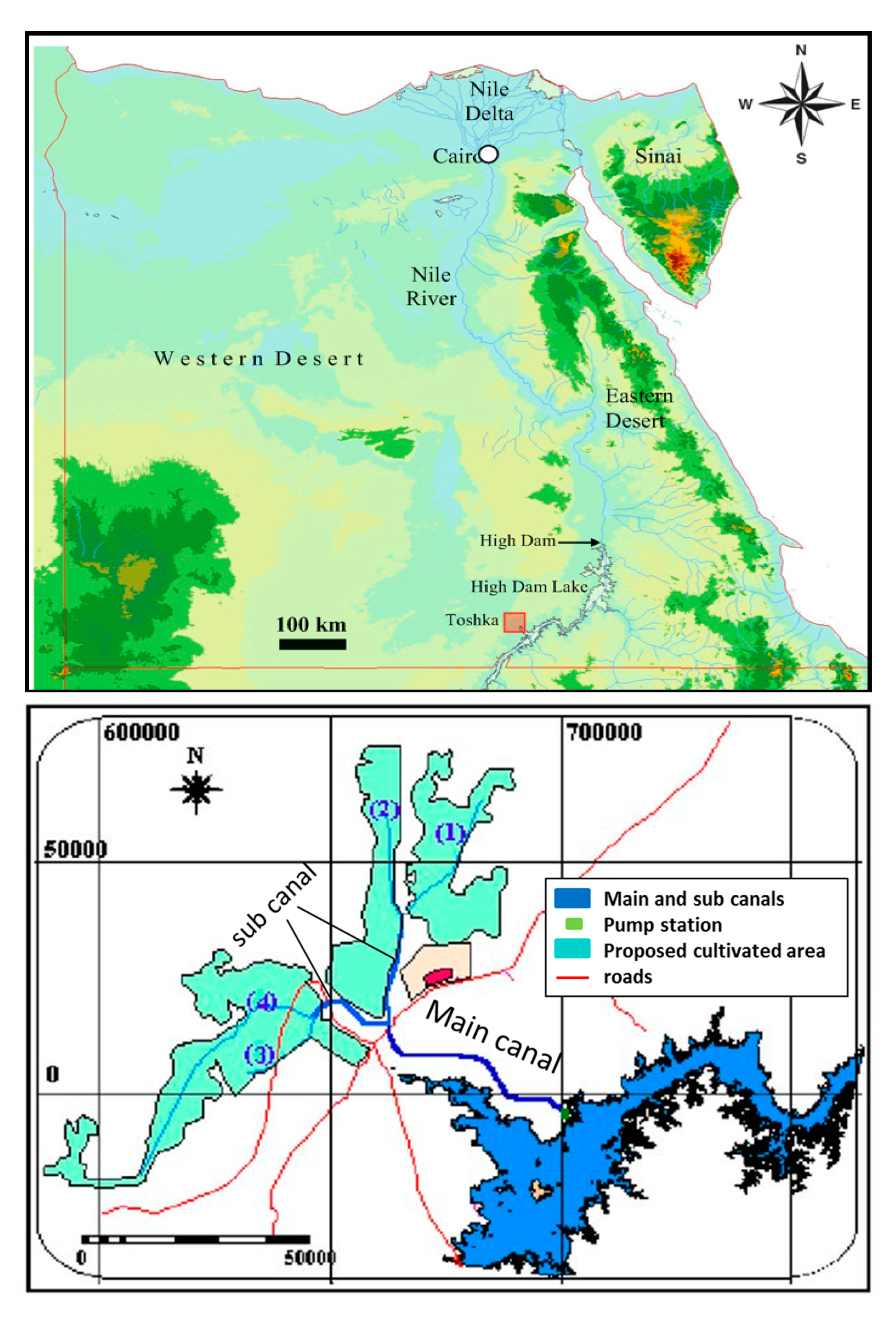
The case study for this research is the Sheikh Zayed Canal in the Toshka area in Egypt. The canal is an artificial concrete lined irrigation canal that starts from Lake Nasser and flows through the western desert, as shown in Figure 1 [10]. The Canal is responsible for conveying water to the 550,000 feddans that will be cultivated as part of the New Valley irrigation project in Toshka. The canal consists of a main channel and several sub-branches with a total length of about 300 km for the whole canal system. The canal system gets its water from Lake Nasser (lake formed behind High Aswan dam) via Mubarak Pumping Station [11]. The canal system has one main canal, two sub-canals, and four sub–sub-canals with the illustrated dimensions in

Table 1. Dimensions of Sheikh Zayed main and sub-canal.

Geometry	Main Canal	Sub-Canal
Wetted Top width	54 m	40 m
Bottom width	30 m	20 m
Water depth	6 m	5 m
Side slopes	2:1	2:1
Length	50 km	22 km

. In this research, the study is concerned only with the main canal and one of the sub-canals (as the two sub-canals have the same dimensions) to show how changing geometry will affect water quality; Figure 1.

2.2. Water Quality Simulation

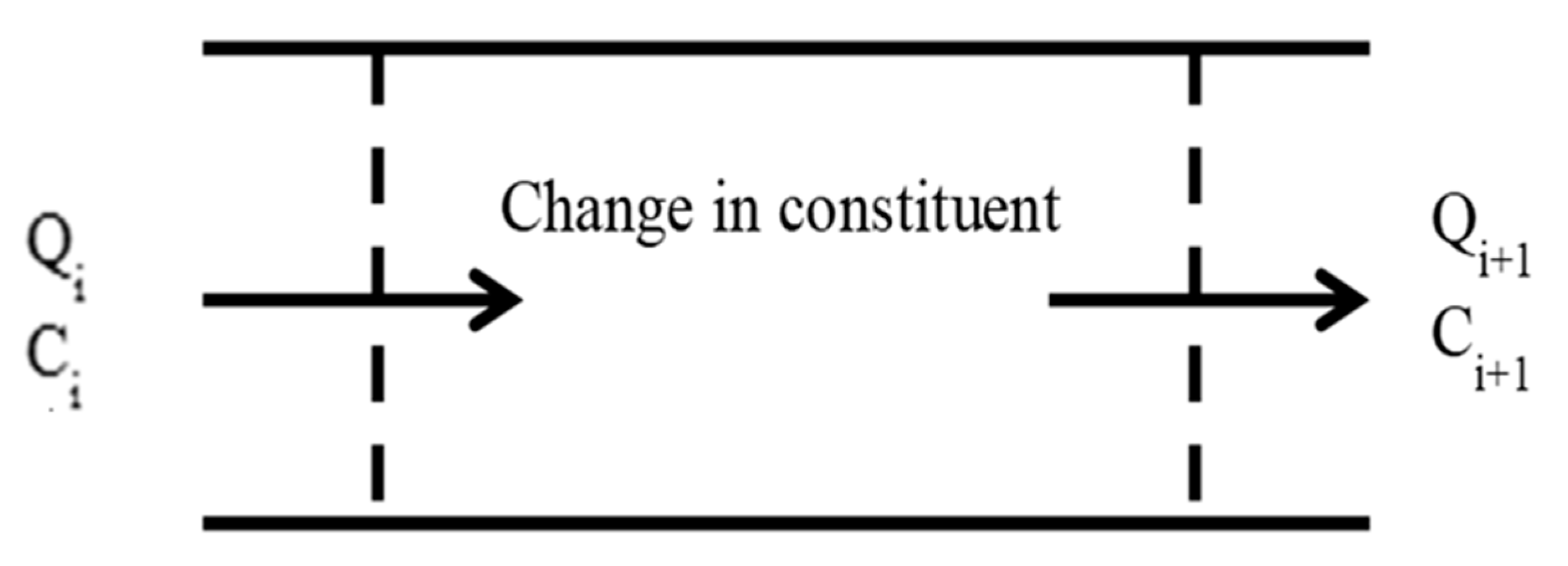
This research is conducted in two parts. In the first part, the effect of changing channel geometry on water quality variables for the main Sheikh Zayed Canal is studied. The original dimensions were studied first and then each geometric parameter is studied itself by changing it. For channel length, the simulations is done for 5000, 10,000, 20,000, 30,000, 40,000, and 50,000 m; for the water depth, the simulation is done for 3, 4, 5, and 6 m; for the bed width, the simulation is done for 5, 10, 15, 20, 25, and 30 m; for side slopes, the simulation is done for side slopes ration of 0, 0.5, 1, 1.5, 2, 2.5. To carry this out, the canal was divided into control volumes; each control volume is 100 m long. The mass balance for each control volume for each water quality variable is modelled as shown in Figure 2. Although the water quality parameters are calculated every 100 m along the 50 km length of the main canal, what is displayed in the results section are the water quality parameters’ concentrations at every 5 km length of the main canal.

The general mass balance equation of all constituents’ concentrations assuming a piston flow is

$$C_{i+1}=C_i+\frac{A\Delta C}{Q_i}dx,$$

(1)

where C_i is initial constituent concentration, C_i+1 is final constituent concentration at the end of control volume, A is cross sectional area, ΔC is the change in constituent concentration, Q_i is discharge at section i, and dx is the length of the control volume.

In the second part of the research, the same simulation was conducted for all water quality variables along the sub-canal and compared to the simulation done for the same variables along the main canal with the initial dimensions in order to study the effect of changing the whole geometry on the water quality.

Therefore, to sum up, two different simulations were done, namely, one simulation addressed the change of each geometric parameter of the main canal, and the other studied its effect on water quality. It must be noted that once a geometric parameter is changed, all other parameters are kept constant. This is to target and assess the effect of this geometric parameter on water quality. For example, when changing the length, all other geometric parameters such as side slopes, widths and depth are kept constant. On the other hand, some geometric parameters if changed will induce a change in other parameters that depend on it like for example the bottom width; if it is changed, it will change the top width with it provided that the depth and side slopes are the same. It should be noted that the results written in Tables 10 to 13 show the changes in geometric parameters are those results of water quality variables at the end section of the 50 km long canal.

The other simulation of this research paper is concerned with changing all geometric parameters together at the same time in order to see the combined effect of their change on the water quality parameters. This was done through simulating the water quality parameters in a sub-branch of the Sheikh Zayed canal that has completely different dimensions than the main canal.

2.3. Water Quality Variables

The water quality variables have been divided into two categories; the first category includes algae, nutrients, TSS, and TDS, which were mathematically modelled using a developed Excel spreadsheet. The second category includes pH, alkalinity, and total inorganic carbon, which were modelled using Python programming language as their calculations are more complicated and iterative [12]. The variables of both categories will be discussed in the following sections.

2.3.1. Algae

The study of algae (a_p) in water is important as excessive growth of algae may cause algae blooms that can result in de-oxygenation of water [13]. Moreover, death and decomposition of this large mass of algae results in depleting even more dissolved oxygen from water. Algae always grow in presence of nutrients. In Lake Nasser, the most common algae groups are Diatoms, Chlophytes, Cyanophytes, and Dinoflagellates. The percentage of each type is 20%, 16.7%, 55.7%, and 7.5%, respectively, throughout the year [14]. It should be noted that average concentration value of all algae types is used in this paper.

Algae concentration increases due to photosynthesis and decreases due to respiration, death, and settling [15]. The change in algae concentration is calculated according to the following equation [16]:

$$S_{ap}=phytoPhoto-phytoResp-phytoDeath-phytoSettl,$$

(2)

where S_ap is algae concentration change over the control volume; phyto_Photo is phytoplankton photosynthesis rate, which is a function of temperature, nutrients, and light. Phyto_Resp is the amount of phytoplankton that is lost due to respiration, and it is function of temperature-dependent phytoplankton respiration/excretion rate and attenuation due to low oxygen. Phyto_Death is the amount of phytoplankton that is lost due to death and depends on temperature, and phyto_Settl is the amount of settled phytoplankton and is a function of settling velocity and water depth.

2.3.2. Nutrients

Modelling nutrients in water is important as at high levels of nutrients, algae may cause algal blooms that can result in de-oxygenation of water. This leads to the death of some aquatic plants and animals [13].

Nutrients include nitrogen and phosphorus compounds. Algae photosynthesis consumes nitrogen in ammonia or nitrate forms and phosphorus in its inorganic phosphate form. If ammonia is the primary nitrogen source, this leads to a decrease in alkalinity because the uptake of positively charged ammonium ions is much greater than the uptake of negatively charged phosphate ions [17]. All nutrients’ calculations are based on the assumption that the organic sediment store in the canal is neglected.

The organic nitrogen increases due to plant death and loss due to hydrolysis and settling. It could be calculated by:

$$S_{no}=f_{onp}{q}_{Np}phytoDeath+f_{onp}{q}_{Np}\frac{BotAlgDeath}{H}-ONHydr-ONSettl,$$

(3)

where f_onp is the fraction of phytoplankton internal nitrogen that is in organic form; q_NP is the cell quotas, which represent the ratios of the intracellular nutrient to the phytoplankton biomass; phyto_Death is the death rate of phytoplankton; BotAlgDeath is the death rate of bottom algae; H is water depth; ONSettl is organic nitrogen settling rate, which is a function of organic nitrogen settling velocity and water depth, and ONHydro is rate of organic nitrogen hydrolysis and is a function of organic nitrogen concentration temperature-dependent organic nitrogen hydrolysis rate.

Ammonia nitrogen (n_a) increases due to hydrolysis of organic nitrogen, in addition to death and excretion of plants, while it decreases via nitrification and plant photosynthesis. The ammonia nitrogen concentration is determined by:

$$\begin{array}{cc}{S}_{na}=& ONHydr+\left(1-f_{onp}\right)q_{Np}phytoDeath+\left(1-f_{onp}\right)q_{Np}\frac{BotAlgDeath}{H}+PhytoExN+\\ & \frac{BotAgExN}{H}-Nitrif-PR{E}_{ap}PhytoUpN-PR{E}_{ab}\frac{BotAlgUpN}{H}-N{H}_{3}GasLoss\end{array}$$

(4)

where ONHydr is the hydrolysis of organic nitrogen, phytoExN is excretion rate of phytoplankton, Nitrif is nitrification rate, PRE_ap is the preference for ammonium as a nitrogen source for phytoplankton, phytoUpN is the intake rate of nitrogen by phytoplankton, PRE_ab is the preference for ammonium as a nitrogen source for bottom algae, BotAlgUpN is the intake rate of nitrogen by bottom algae, and NH₃GasLoss is the NH₃ gas loss into air.

The nitrate nitrogen (n_n) increases due to nitrification of ammonia while it is lost due to de-nitrification and plant uptake. The nitrification and de-nitrification rates are calculated by:

$$S_{ni}=Nitrif-Denitr-\left(1-P_{ab}\right)\frac{BotAlgUpN}{H},$$

(5)

where Denitr is the de-nitrification rate of nitrate nitrogen, and P_ab is the preference for ammonium as a nitrogen source for bottom algae.

$$Denitr=\left(1-F_{oxdn}\right)k_{dn}\left(T\right)n_n,$$

(6)

where k_dn(T) is a temperature-dependent de-nitrification rate of nitrate nitrogen [d⁻¹], and F_oxdn is the effect of low oxygen on de-nitrification [dimensionless].

The organic phosphorus (p_o) increases due to plant death and excretion while it is lost through hydrolysis and settling. The organic phosphorus and hydrolysis rates are calculated by:

$$S_{Po}=f_{oPP}{q}_{Pp}\frac{PhytoDeath}{H}+f_{oPb}\frac{BotAlgDeath}{H}-OPHydr-OPSettl,$$

(7)

where f_opp is the fraction of the phytoplankton internal phosphorus that is in organic form, q_pp is the phytoplankton cell quotas of phosphorus [mgP/mgA], and it is calculated as q_pp = IP_p/a_p; OPHydro is the organic phosphorus hydrolysis rate and is a function of fraction of phytoplankton internal phosphorus that is in organic form and temperature-dependent organic phosphorus hydrolysis rate; OPSettl is the organic phosphorus settling rate, and it depends on organic phosphorus settling velocity and water depth.

The concentration of inorganic phosphorus (P_i) increases due to organic phosphorus hydrolysis and plant excretion while it is lost due to plant uptake. Furthermore, a settling loss is included for cases in which inorganic phosphorus is lost due to sorption onto settle-able particulate matter.

$$\begin{array}{cc}{S}_{Pi}=& OPHydr+\left(1-f_{oPP})q_{Pp}PhytoDeath+(1-f_{oPb}\right)q_{Pp}\frac{BotAlgDeath}{H}+PhytoExP+\\ & \frac{BotAlgExP}{H}-PhytoUpP-\frac{PhytoUpP}{H}-IPSettl,\end{array}$$

(8)

where IPSettl is the internal phosphorus settling, and it depends on inorganic phosphorus settling velocity and water depth.

2.3.3. Total Suspended Solids

Total Suspended Solids (TSS) are solids in water that can be trapped by a filter. The main source of TSS in Lake Nasser is the incoming sediment from the Ethiopian highlands during flood [18]. In this research, the TSS is modeled at the maximum flood period during August. TSS concentration at every cross section is calculated using mass balance equation assuming that it is controlled by inorganic settling of sediments only assuming no re-suspension of sediment store in the canal; the relation between the TSS and flow rate is explained in Equation (1). The inorganic settling is calculated by [15]:

$$InorgSettl=\frac{v_i}{H}{m}_i,$$

(9)

where v_i is the inorganic suspended solids settling velocity [m/d]. H is the water depth [m], and m_i is the mass of suspended sediments.

2.3.4. Total Dissolved Solids

Total Dissolved Solids (TDS) is a measure of all dissolved substances in water. TDS is a significant water quality variable that should be assessed as it affects the aquatic fauna and flora, which are adapted to a certain specific salinity range. The TDS concentration is calculated based on the assumption that the evaporation rate is the main influencer, and no account for chemical reactions is taken. Thus, the evaporation rate is calculated using the widely used model, Penman–Monteith, which is based on a comparison between three evaporation models. This model gave the most accurate results, and this comparison is in a paper published before [7]. The metrological data used in evaporation calculations are in average daily form and are observed at the Aswan weather station near Toshka. The calculation procedure was obtained based on the mass balance equation that will be mentioned later in the methodology section, and the TDS concentration is determined at the end section of the channel.

2.3.5. pH

pH of water defines the solubility and biological availability of chemical constituents in water such as nutrients and heavy metals, and it affects the aquatic life. The pH is determined by:

$$pH=-lo{g}_{10}\left[H^{+}\right],$$

(10)

Considering the change of pH through the channel by assuming constant volumetric flow, the root of the equation is determined numerically using Newton–Raphson method [19]:

$$f\left(\left[H^{+}\right]\right)=\left({\propto }_1+2{\propto }_2\right)C_T+\frac{K_w}{\left[H^{+}\right]}-\left[H^{+}\right]-Alk,$$

(11)

where [H⁺] is the hydronium ion density; α₁ and α₂ are the fraction of total inorganic carbon in bicarbonate and carbonate, respectively; C_T is the total inorganic carbon concentration; K_w is the acidity constant; and Alk is the alkalinity of water.

2.3.6. Alkalinity

Algae photosynthesis consumes nitrogen in ammonia or nitrate forms and phosphorus in its inorganic phosphate form. If ammonia is the primary nitrogen source, this leads to a decrease in alkalinity because the uptake of positively charged ammonium ions is much greater than the uptake of negatively charged phosphate ions [16]. If nitrate is the primary nitrogen source, then alkalinity will increase because both nitrate and phosphate are negatively charged. The change in alkalinity (Alk) in the mass balance equation is solved by:

$$ds={Sa}_{nit}+{Sa}_{denit}+{Sa}_{ONh}+{Sa}_{Oph}+{Sa}_{phytp}+{Sa}_{phytup}+{Sa}_{pEx},$$

(12)

where ds is change in alkalinity in the control volume, Sa_nit is change in alkalinity due to nitrification, Sa_denit is change in alkalinity due to de-nitrification, Sa_ONh is change in alkalinity due to hydrolysis of organic nitrogen, Sa_Oph is change in alkalinity due to organic phosphorus hydrolysis, Sa_phytp is change in alkalinity due to algae photosynthesis, Sa_phytup is change in alkalinity due to algae nutrients excretion, and Sa_pEx is alkalinity change due to algae nutrients uptake.

2.3.7. Total Inorganic Carbon

Total inorganic carbon concentration (CT) increases due to fast carbon oxidation and algae respiration while it is lost through algae photosynthesis. Based on the condition of water whether it is under-saturated or oversaturated with, it is gained or lost through re-aeration; it is calculated as [6]:

$$dCT=r_{ccc}FastCOxid+r_{cca}PhytoResp-r_{cca}PhytoPhoto+{CO}_{2}Rear,$$

(13)

where r_ccc and r_cca are stoichiometric ratios; they are determined by Laws and Chapra [20,21], FastCOxid is to fast carbon oxidation rate, and CO₂Rear is the CO₂ re-aeration rate and is function of temperature-dependent carbon dioxide re-aeration coefficient and saturation concentration of carbon dioxide.

2.4. Initial Concentrations and Flow Data

The initial concentrations of the modelled water quality variables of Sheikh Zayed main canal are measured and recorded by the Ministry of Water Resources and Irrigation in Egypt. The samples are taken from the inlet of the Sheikh Zayed canal at the nearest station on Lake Nasser (Toshka station). The initial values of water quality variables for the main canal are shown in

Table 2. Initial concentration of the studied water quality parameters.

Water Quality Variable	Initial Value	Unit
Algae (ap)	6.34	μg/L
Organic Nitrogen (no)	700.00	μg/L
Ammonia Nitrogen (na)	50.53	μg/L
Nitrate Nitrogen (nn)	469.00	μg/L
Organic phosphorus (po)	18.15	μg/L
Inorganic phosphorus (pi)	73.46	μg/L
Total Suspended Solids (TSS)	56.00	mg/L
Total Dissolved Solids (TDS)	160.00	mg/L
pH	7.70	-
Alkalinity (Alk)	2.24	meq/L
Total Inorganic Carbon (CT)	2.30	mMol/L

[22]; however, the initial values for the sub-canal are taken from the simulation of the main canal at the end section where the sub-canal is branching. The pumping station providing the main canal has a flow rate of 300 m³/s, and flow velocity in the main canal is 1.2 m/s. On the other hand, the sub-canal has a flow rate of 150 m³/s and flow velocity of 1.02 m/s. It should be noted that the flow velocity is changed by the changing geometric dimensions of the canal; for example, decreasing the water depth will increase the flow velocity because the cross sectional area is changed, but the flow rate is constant as the pumping station provides a constant flow rate. The constants used in all calculations are the same values as those used in Qual2K computer package, shown in

Table 3. Values of constants used in the modeling.

Constant	Value	Unit	Description
Max uptake rate of nitrogen	1.06	mgN/mgA/d	The maximum uptake rate for nitrogen
KqNP	2.00	μgN/L	Half-saturation constant for intracellular nitrogen
KsNP	15.00	μgN/L	Half-saturation constant for external nitrogen
qoNp	0.07	mgN/mgA
qNP	0.17	mgN/mgA
Kep	0.01	d-1	The temperature-dependent bottom algae excretion rate
Kd	0.25	d-1	Phytoplankton death rate
Kqpp	0.20	μgP/L	Half-saturation constant for intracellular phosphorus
Kspp	2.00	μgP/L	Half-saturation constant for external phosphorus
Max uptake rate of Phosphorus	0.15	mgP/mgA/d
qoPp	0.01	mgP/mgA
qPp	0.02	mgP/mgA
Ke	0.68	m-1	Light extinction coeff
KLP	50.00	langleys/d	Phytoplankton light parameter
Kgp	2.50	d-1	Max Photosynthesis rate
Krp	0.13	d-1	Phytoplankton respiration/excretion rate
υa	0.15	m/d	Phytoplankton settling velocity
khn	0.05	d-1	Temperature dependent organic nitrogen hydrolysis rate
von	0.05	m/d	Organic nitrogen settling velocity
kn(T)	1.00	d-1	Nitrification rate for ammonia nitrogen
ksona	0.60	l/mg	Half saturation constant for the effect of low oxygen on nitrification
Foxna	0.91	dimensionless	Attenuation due to low oxygen
khnxp	25.00	ugN/L	Ammonia preference
Ksodn	0.60	l/mg	Half saturation constant for the effect of low oxygen on denitrification
kdn	1.00	d-1	Denitrification rate for ammonia nitrogen
Foxdn	0.91	dimensionless	Effect of low oxygen on denitrification
khp	0.05	m/d	Organic phosphorus hydrolysis rate
vop	0.05	m/d	Organic phosphorus settling velocity
vip	0.05	m/d	Inorganic phosphorus settling velocity

, as those values do not change much from one case to another. In addition, it should be noticed that the hydrodynamic simulation in this research was conducted using the Manning equation as follows:

Q = (1.49/n) A R ^(2/3) S ^(1/2),

(14)

where Q is the flow rate (m³/s), n is Manning’s Roughness Coefficient (unitless), A is the sectional area (m²), R is the hydraulic radius (m), and S is the bed slope.

2.5. Model Calibration

The constructed mathematical models are calibrated for the original geometry of Sheikh Zayed Canal as well as for the minimum and maximum conditions of change of each geometric parameter of this canal (i.e., if depth is checked from 3 m to 6 m every 1 m, then calibration is made for the depth of 3 m and of 6 m to make sure the calibration results hold in every case).

Water quality variables and their calibration are divided into three categories; the first category includes algae, nutrients, and TSS and is calibrated against Qual2k water quality model. Qual2K is a modelling framework for simulating river and stream water quality developed by Chapra [16]. It is implemented within the Microsoft Windows environment, and it was validated and calibrated many times by many researchers who found it to be a reliable computer package [23,24]. Therefore, it could be concluded that Qual2K is a reliable method for calibration of results of this research paper. The second category includes TDS, which is calibrated against site observations obtained by the Ministry of Water Resources and Irrigation at Toshka station on Lake Nasser, and the third category includes pH, alkalinity, and CT that are calibrated with numerical example developed by Chapra in his book [21] as shown in

Table 4. Water quality variables calibration results for the main canal with its original dimensions.

Water Quality Variables	Constructed Model Outputs	Reference Value	% Error
ap (μg/L)	6.38	6.52	2.21
na (μg/L)	120.32	120.50	0.15
no (μg/L)	1556.68	1557.48	0.05
Pi (μg/L)	73.45	73.54	0.13
Po (μg/L)	18.10	18.11	0.06
TSS (mg/L)	56.17	56.05	0.21
TDS (mg/L)	140.08	140.00	0.001
pH	6.61	6.60	0.20
CT (mMol/L)	0.003	0.003	0.01

.

As it could be noted from Table 4, the % error is very negligible due to inaccuracy in real measured data and/or from the assumptions of some constants.

As mentioned before, the mathematical model is also calibrated against the Qual2k model for the minimum simulated geometry as shown in

Table 5. Calibration with Qual2k for water depth 3 m.

Water Quality Variables	Constructed Model Outputs	Reference Value	% Error
ap (μg/L)	6.55	6.43	1.83
na (μg/L)	52.29	52.39	0.19
nn (μg/L)	469.27	471.26	0.42
no (μg/L)	690.56	695.89	0.77
po (μg/L)	17.90	18.04	0.77
Pi (μg/L)	73.67	73.67	0.00
Alk (meq/L)	2.25	2.22	1.12
pH	6.49	6.62	1.97
TSS (mg/L)	56.17	56.32	0.27
TDS (mg/L)	240.00	240.00	0.00
Average			0.73

,

Table 6. Calibration with Qual2k for bed width 5 m.

Water Quality Variables	Constructed Model Outputs	Reference Value	% Error
ap (μg/L)	6.38	6.32	0.93
na (μg/L)	52.21	52.28	0.13
nn (μg/L)	469.24	471.14	0.40
no (μg/L)	692.21	696.16	0.57
po (μg/L)	17.94	18.05	0.59
Pi (μg/L)	73.53	73.65	0.16
Alk (meq/L)	2.25	2.22	1.17
pH	6.92	7.02	1.42
TSS (mg/L)	56.16	56.58	0.75
TDS (mg/L)	240.00	240.00	0.00
Average			0.61

,

Table 7. Calibration with Qual2k for side slopes 0 (rectangular cross section).

Water Quality Variables	Constructed Model Outputs	Reference Value	% Error
ap (μg/L)	6.41	6.40	0.15
na (μg/L)	53.34	52.31	1.96
nn (μg/L)	469.28	471.16	0.40
no (μg/L)	686.31	696.08	1.40
po (μg/L)	17.79	18.05	1.45
Pi (μg/L)	73.59	73.66	0.09
Alk (meq/L)	2.25	2.22	1.28
pH	6.65	6.72	1.11
TSS (mg/L)	56.28	56.32	0.08
TDS (mg/L)	240.00	240.00	0.00
Average			0.79

and

Table 8. Calibration with Qual2k for channel length 5000 m.

Water Quality Variables	Constructed Model Outputs	Reference Value	% Error
ap (μg/L)	6.35	6.35	0.05
na (μg/L)	50.96	52.39	2.72
nn (μg/L)	469.02	471.26	0.48
no (μg/L)	698.07	695.89	0.31
po (μg/L)	18.10	18.13	0.17
Pi (μg/L)	73.48	73.67	0.26
Alk (meq/L)	2.24	2.22	0.96
pH	7.40	7.50	1.29
TSS (mg/L)	56.04	56.59	0.97
TDS (mg/L)	240.02	240.00	0.01
Average			0.72

.

The Egyptian Ministry of Water resources calibrates the mathematical model against water quality variables observations and Irrigation and Qual2k model for the original dimensions of the main Sheikh Zayed Canal and the minimum selected geometry. Therefore, it is reliable to calculate, model, and predict the required data for the research.

3. Results

3.1. Main Canal Simulation

The water quality variables were simulated along the main canal with its initial dimensions according to the methodology discussed before as shown in

Table 9. Main canal simulation results.

Water Quality Variable	Length (m)
	0	5000	10,000	20,000	30,000	40,000	50,000
ap (μg/L)	6.338	6.347	6.357	6.377	6.397	6.418	6.438
no (μg/L)	700	698.066	696.138	692.299	688.482	684.688	680.915
na (μg/L)	50.533	50.964	51381	52.178	52.924	53.621	54.27
nn (μg/L)	469	469.016	469.038	469.091	469.151	469.211	469.265
Po (μg/L)	18.15	18.099	18.048	17.946	17.845	17.745	17.645
Pi (μg/L)	73.46	73.478	73.496	73.532	73.569	73.607	73.646
TSS (mg/L)	56	56.039	56.077	56.155	56.232	56.31	56.388
TDS (mg/L)	160	160.015	160.029	160.058	160.088	160.117	160.146
pH	7.7	7.403	7.155	6.879	6.715	6.593	6.497
Alk (meq/L)	2.24	2.241	2.243	2.245	2.247	2.249	2.249
CT (mMol/L)	2.3	2.445	2.59	2.88	3.17	3.46	3.758

.

3.1.1. Water Depth

Different water depths (d) were assumed to be ranged from the original designed depth of 6 m and then decreasing by one-meter increment until reaching a final depth of 3 m; then, the water quality variables were simulated as shown in

Table 10. Effect of water depth (d) on different water quality variables.

Variables	Depth (m)
	6	5	4	3
B (m)	54	50	46	42
Area (m2)	252	200	152	108
ap (μg/L) no (μg/L)	6.438 680.91	6.532 684.37	6.569 687.59	6.547 690.56
na (μg/L)	54.27	53.59	52.93	52.289
nn (μg/L)	469.265	469.268	469.302	469.303
Po (μg/L)	17.645	17.737	17.822	17.902
Pi (μg/L)	73.65	73.66	73.66	73.67
TSS (mg/L)	56.388	56.31	56.236	56.168
TDS (mg/L)	160	160	160	160
pH	6.497	6.497	6.496	6.49
CT (mMol/L)	3.76	3.75	3.75	3.77
Alk (meq/L)	2.249	2.248	2.247	2.245

, which also showed that as the depth decreases, the top width also decreases.

The results indicated that the algae concentration is slightly influenced by the water depth, since by decreasing the water depth, the algae concentration increases from 6.438 to 6.547 μg/L (Table 10, row 3). Although slightly affected, it is noted that algae were affected by changing water depth more than the other variables. These results can be explained since the sunlight that penetrates water increases with the decrease of water depth. It should be noted that the flowing conditions, which is a factor affecting the growth of algae, are constant as mentioned before.

In addition, the results showed that the organic nutrients such as organic nitrogen and phosphorus concentrations are inversely proportional to water depth due to the algae uptake of nutrients. Although the nitrate nitrogen and inorganic phosphorus are also inversely proportional to the water depth, they are less affected by changing the depth. The organic nitrogen concentration ranged from 680.91 to 690.56 μg/L (Table 10, row 4) while the ammonia nitrogen concentration ranged from 52.289 to 54.27 μg/L (Table 10, row 5) corresponding to the studied water depth. It could be noticed that the nitrate nitrogen, which ranged from 469.265 to 469.268 μg/L (Table 10, row 6), is slightly affected by the water depth as well as the inorganic phosphorus that ranges from 73.65 to 73.67 μg/L (Table 10, row 7).

The TSS concentration at the main canal is strongly affected by algae, as its main influencer is the organic and inorganic settling, which is directly affected by water depth, so the TSS concentration decreases as the water depth decreases. According to the results, TSS concentration ranged from 56.388 to 56.168 mg/L (Table 10, row 8) for the water depth ranging from 6 m to 3 m. On the other hand, it could be noted that the water depth does not affect TDS concentrations.

The alkalinity and the total inorganic carbon are very slightly affected by the water depth. The alkalinity is directly proportional to the water depth while the total inorganic carbon is inversely proportional to the water depth. As for pH, it is directly proportional to the water depth. The pH changed in a very narrow range from 6.490 to 6.497 (Table 10, row 9); the same was true for the alkalinity, which ranged from 2.245 and 2.249 meq/L (Table 10, row 11). As for the total inorganic carbon, it also changed slightly from 3.774 to 3.758 mMol/L (Table 10, row 10).

3.1.2. Bed Width

The bed width (b) varies from the original canal bed width, which is 30 m and incrementally decreased, by 5 m, to 5 m while the channel side slopes, and water depth is kept constant. The changes in the concentrations of the studied water quality variables by changing the bed width are summarized in

Table 11. Effect of bed width (b) on different water quality variables.

Variables	Bed Width (b) (m)
	30	25	20	15	10	5
Area (m2)	252	222	192	162	132	102
ap (μg/L)	6.44	6.43	6.41	6.4	6.39	6.38
no (μg/L)	680.91	683.16	685.41	687.67	689.93	692.21
na (μg/L)	54.27	53.89	53.5	53.09	52.66	52.21
nn (μg/L)	469.26	469.28	469.29	469.28	469.26	469.24
Po (μg/L)	17.64	17.7	17.76	17.82	17.88	17.94
Pi (μg/L)	73.65	73.62	73.6	73.58	73.55	73.53
TSS (mg/L)	56.39	56.34	56.3	56.25	56.2	56.16
TDS (mg/L)	160	160	160	160	160	160
pH	6.50	6.56	6.62	6.70	6.80	6.92
CT (mMol/L)	3.76	3.57	3.39	3.20	3.01	2.83
Alk (meq/L)	2.249	2.249	2.249	2.248	2.247	2.250

.

The algae concentration is directly proportional to the bed width; that is because, by decreasing the bed width, the top width and the volume of the surface layer decrease causing a decrease in the solar radiation penetration, which is important for the photosynthesis process of algae. The algae concentration ranged from 6.44 μg/L to 6.38 μg/L (Table 11, row 2). The same effect was noticed in case of ammonia, nitrate nitrogen and inorganic phosphorus. However, the results showed that organic nitrogen and phosphorus increased by decreasing the bed width. The organic nitrogen concentration ranged from 680.91 to 692.21 μg/L (Table 11, row 3); while the organic phosphorus ranged from 17.64 to 17.94 μg/L (Table 11, row 6). On the other hand, the minimum value of TSS was recorded to be 56.16 mg/L at the minimum bed width and the maximum value of TSS was recorded to be 56.39 mg/L at the maximum bed width (Table 11, row 8). These results are expected due to the decrease of algae concentration causing in decreasing the settled decayed number of algae, which resulted in increasing the TSS concentration.

The pH was inversely proportional to the bed width and ranged from 6.92 to 6.497 (Table 11, row 10). Furthermore, the alkalinity results showed a slight inverse proportional relation with the bed width and ranged from 2.25 to 2.249 meq/L (Table 11, row 12). While the total inorganic carbon results showed a direct proportional relationship with bed width and ranged from 2.83 to 3.758 mMol/L (Table 11, row 11).

3.1.3. Side Slopes

The modelled ratio of side slopes (Ss) (horizontal to vertical) ranges from 0, which reflects a rectangular cross section, to 2.5; while the original side slopes ratio of the canal is 2 (2:1). The side slopes ratio is changed with respect to a constant value of bed width, which is the initial bed width of the canal, and as a result, when the side slopes are changed, the bed width (b) remains constant, but the top width (B) changes, as shown in

Table 12. Effect of side slopes (Ss) on different water quality variables.

Variables	Side Slope (Ss) (m/m)
	2.5	2	1.5	1	0
b (m)	30	30	30	30	30
B (m)	60	54	48	42	30
Area (m2)	270	252	234	216	180
ap (μg/L)	6.45	6.44	6.43	6.42	6.41
no (μg/L)	679.57	680.91	682.26	683.61	686.31
na (μg/L)	54.49	54.27	54.05	53.82	53.34
nn (μg/L)	469.26	469.26	469.27	469.27	469.28
Po (μg/L)	17.61	17.64	17.68	17.72	17.79
Pi (μg/L)	73.66	73.65	73.63	73.62	73.59
TSS (mg/L)	56.42	56.39	56.36	56.33	56.28
TDS (mg/L)	160.00	160.00	160.00	160.00	160.00
pH	6.47	6.497	6.525	6.559	6.65
CT (mMol/L)	3.848	3.758	3.665	3.565	3.33
Alk (meq/L)	2.25	2.249	2.249	2.249	2.248

.

The algae concentration is directly proportional to the canal side slopes. The maximum-modelled ratio of side slopes (2.5) corresponds to a maximum concentration of algae 6.45 μg/L while the minimum ratio of side slopes corresponds to a minimum concentration of algae 6.41 μg/L (Table 12, row 4). On the other hand, organic nitrogen and phosphorus are inversely proportional to the side slopes; the organic nitrogen ranged from 679.57 to 686.31 μg/L (Table 12, row 5), and organic phosphorus ranged from 17.61 to 17.79 μg/L (Table 12, row 8). The ammonia nitrogen ranged from 54.49 to 53.34 μg/L. While the nitrate nitrogen and inorganic phosphorus are the least affected nutrient compounds as the nitrate nitrogen ranged from 469.26 to 469.28 μg/L (Table 12, row 7), and the inorganic phosphorus ranged from 73.66 to 73.59 μg/L (Table 12, row 9).

The TSS concentration is directly proportional to the side slope. At minimum side slope, which corresponds to a rectangular cross section, the TSS concentration is 56.28 mg/L; while at the maximum side slop the TSS is 56.42 mg/L (Table 12, row 10).

The pH is decreasing by increasing the side slope, and the pH ranged from 6.65 to 6.47 (Table 12, row 12). Otherwise, the alkalinity slightly decreases with decreasing side slopes. In addition, the total inorganic carbon is also decreasing with decreasing side slope. It ranged from 3.848 to 3.33 Mmol/L (Table 12, row 13).

3.1.4. Channel Length

The effect of changing the canal length on different water quality variables is summarized in

Table 13. Effect of channel length on the water quality variables.

Variables	Length (m)
	50,000	40,000	30,000	20,000	10,000	5000
ap (μg/L)	6.44	6.42	6.4	6.38	6.36	6.35
no (μg/L)	680.91	684.69	688.48	692.3	696.14	698.07
na (μg/L)	54.27	53.62	52.92	52.18	51.38	50.96
nn (μg/L)	469.26	469.21	469.15	469.09	469.04	469.02
Po (μg/L)	17.64	17.74	17.85	17.95	18.05	18.1
Pi (μg/L)	73.65	73.61	73.57	73.53	73.5	73.48
TSS (mg/L)	56.39	56.31	56.23	56.15	56.08	56.04
TDS (mg/L)	160.15	160.12	160.09	160.06	160.03	160.01
pH	6.50	6.59	6.72	6.88	7.16	7.40
CT (mMol/L)	3.758	3.46	3.17	2.88	2.59	2.45
Alk (meq/L)	2.249	2.249	2.247	2.245	2.243	2.241

. The studied canal length values are 5000, 10,000, 20,000, 30,000, 40,000, and 50,000 m.

The algae concentration is directly proportional to the canal length because as the length increases, the water surface area increases, and thus, the penetration of sun increases. The algae concentration ranged from 6.35 μg/L to 6.44 μg/L (Table 13, row 1). The organic nitrogen ranged from 698.07 to 680.91 μg/L (Table 13, row 2), the ammonia nitrogen ranged from 50.96 to 54.27 μg/L (Table 13, row 3), and the nitrate nitrogen ranged from 469.02 to 469.26 μg/L (Table 13, row 4). In addition, the organic phosphorus ranged from 18.10 to 17.64 μg/L (Table 13, row 5), and the inorganic phosphorus ranged from 73.48 to 73.65 μg/L (Table 13, row 6), which represents the slightest change over all the nutrient compounds.

The TSS concentration is expected to increase with the canal length increase because of the organic settling that increases with the algae increase. The maximum TSS concentration 56.39 mg/L was recorded at the maximum canal length and the minimum TSS concentration 56.04 mg/L was recorded at the minimum canal length (Table 13, row 7). On the other side, the TDS is slightly affected by the canal length and it ranged from 160.015 to 160.146 mg/L (Table 13, row 8). This change may be neglected in comparison with the huge canal length.

In addition, it can be noticed that the canal length has a considerable effect on pH and total inorganic carbon while it has a minor effect on alkalinity. The pH ranged from 7.403 to 6.497 (Table 13, row 9), while the alkalinity ranged from 2.241 to 2.249 meq/L (Table 13, row 11), and the total inorganic carbon ranged from 2.445 to 3.758 mMol/L (Table 13, row 10).

3.2. Sub-Canal Simulation

The simulation results for one of the sub-branches of Sheikh Zayed Canal are summarized in

Table 14. Sub-canal water quality simulation results.

Variables	Length (m)
	0	5000	10,000	15,000	20,000	22,000
ap (μg/L)	6.438	6.466	6.495	6.525	6.555	6.567
no (μg/L)	680.915	678.612	676.32	674.035	671.759	670.851
na (μg/L)	54.270	54.633	54.981	55.311	55.626	55.747
nn (μg/L)	469.265	469.291	469.311	469.324	469.329	469.330
Po (μg/L)	17.645	17.584	17.523	17.463	17.403	17.379
Pi (μg/L)	73.646	73.676	73.707	73.738	73.770	73.783
TSS (mg/L)	56.388	56.434	56.480	56.526	56.572	56.591
TDS (mg/L)	160.146	160.168	160.189	160.211	160.233	160.241
pH	6.497	6.446	6.404	6.363	6.325	6.312
CT (mMol/L)	2.249	2.250	2.251	2.251	2.252	2.252
Alk (meq/L)	3.758	3.938	4.119	4.299	4.480	4.552

. The sub-branch length is 22 km, its flow rate is 150 m³/s, and the calculated flow velocity based on the flow rate and sub- canal geometry is 1.02 m/s.

The starting water quality variables’ concentrations of the sub-canal are the end concentrations simulated at the end section of the main 50 km length canal.

It could be realized from the sub-canal results that by decreasing the water depth to 5 m, top width to 40 m, and bottom width to 20 m, the algae concentration increased to 6.567 μgA/L (Table 14, row 1), the organic nitrogen decreased to 670.851 μgN/L (Table 14, row 2), the ammonia nitrogen increased to 55.747 μgN/L (Table 14, row 3), and nitrate nitrogen increased to 469.330 μgN/L (Table 14, row 4). In addition, the phosphorus compounds slightly changed in the sub-branch as the organic phosphorus decreased to 17.379 μgP/L (Table 14, row 5), and the inorganic phosphorus increased to 73.783 μgP/L (Table 14, row 6). However, the pH decreased to 6.312 (Table 14, row 9) while the total inorganic carbon increased to 4.552 mMol/L (Table 14, row 10).

4. Discussion and Conclusions

Although there are some research studies assessing the effect of some parameters such as the existence of dams, barrages, and covering of canals on some water quality variables, the effect of geometric characteristics was not extensively studied before. This research paper is concerned with studying the effect of channel geometry on many water quality variables.

The simulation was done twice, once for the main canal by changing each geometric parameter and assessing its effect on water quality and other time by changing all geometric parameters at the same time in order to assess the combined effect of this change and also to prove that water quality variables change from main canals to sub-branches of those canals. This will aid in decision making—from a water quality point of view—regarding which canal to use more in irrigation of crops or even for drinking purposes—after treatment.

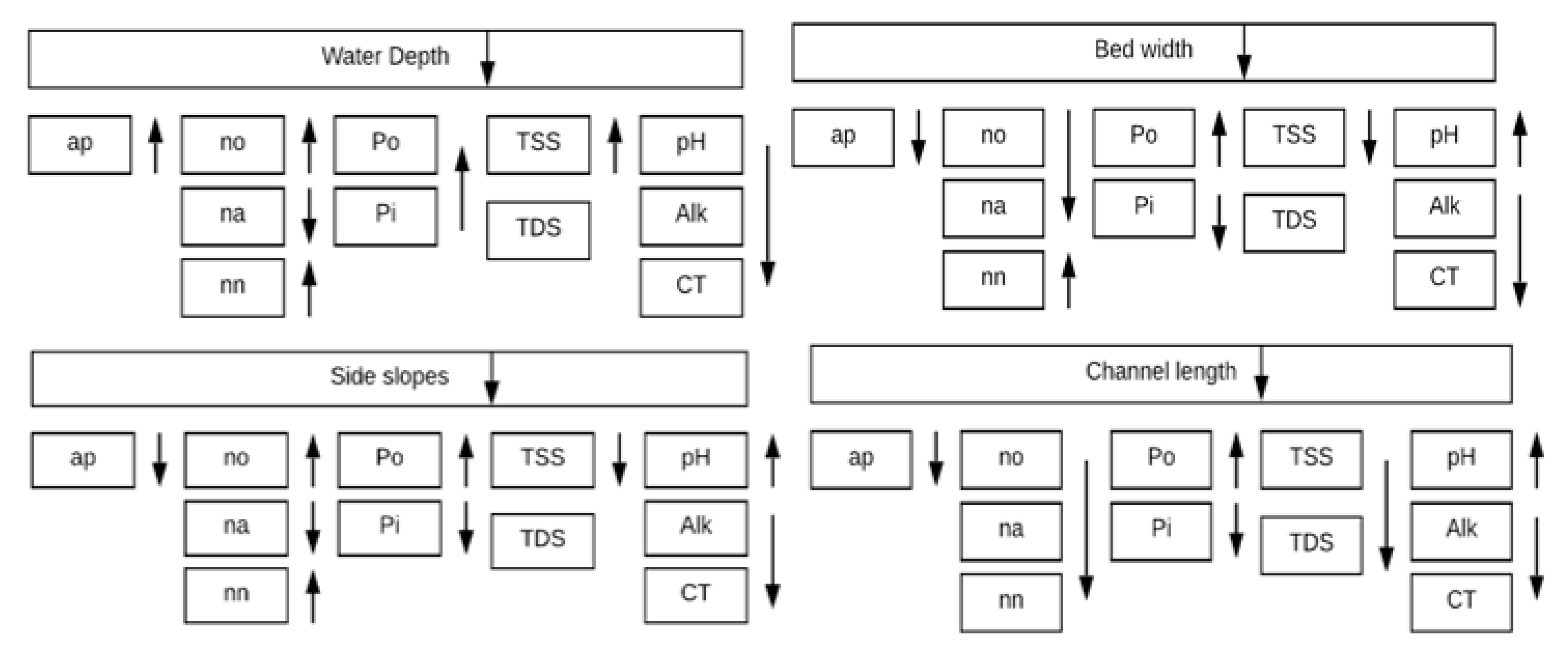
It could be concluded out of this research study that changing the geometry of a canal has an impact on its water quality. The studied water quality variables of the Sheikh Zayed Canal are in general slightly affected, but still some of those variables are affected more than others. The impact of change of each geometric characteristic on the studied water quality variables is summarized in Figure 3.

It could be realized from the results that the algae concentration is affected by the changing geometry; by changing the length between 5000 and 50,000 m and the water depth between 6 and 3 m, the algae increased by 2%, while by changing the bed width between 5 and 30 m and the side slopes between 0 and 2.5, the algae concentration decreased by 1%. The percentage change of algae is highly affected by the initial algal count, which is too small in this case. In other cases, the % change is expected to be greatly affected when the algal count is high. The pH is significantly affected by changing geometry; for the main canal, the pH decreased by 13% by changing length between 5000 m and 50,000 m, it is increased by 7% for changing bed width between 5 and 30 m, it increased by 3% when changing side slopes between 0 and 2.5 m, while it is not affected by changing the water depth. For the sub-canal, the pH decreased by 2% when changing length between 5000 m and 22,000 m. As for the total carbon, it increased by 64% for the length change; it decreased by 25% for the bed width change; it decreased by 14% for the side slopes change, and it is not affected by water depth. Moreover, the total nitrogen, total phosphorus, and alkalinity have not considerably changed by changing channel geometry.

Though the case study for this research was selected to be Sheikh Zayed canal in Toshka, the study results could generally be applied to any waterway anywhere if the hydrologic and meteorological conditions of the waterway are provided. The hydrologic conditions are volume flow rate, water velocity, and channel geometry, while the meteorological conditions are air temperature, atmospheric pressure, shortwave, wind speed, etc.

It could be expected that mathematically simulated variables’ concentrations of studied canals could vary more with changing geometry—but following the same trend—if the studied canal is heavily polluted more than the case study canal in this research paper. It is also worth to mention that in case of other larger canals or branches of rivers, where the volume flow rate is greater and the geometry is larger than the studied canal, the effect of changing canal geometry may impact water quality variables more significantly but with the same trend as found in this research study, and thus, the findings of this study could generally be applied on any waterway. Finally, the importance of studying the effect of canal geometry on water quality variables may be used as an assessment tool—from the water quality point of view—aiding designers when comparing different sizes of canals before construction. Moreover, when designing the river or canal waste allocation plan, the effect of geometry should be studied because the geometry of those waterways changes constantly due to silt deposit and erosion, and thus, the water quality variables are affected. Therefore, it is recommended to assess the effect of geometry of waterways on water quality variables in order to take it into consideration when designing the waste allocation plan for a certain waterway.

From the water quality simulation of the sub-canal, it could be observed that when all geometric parameters of a canal change at the same time, the behavior of the water quality variables’ concentrations will not be the same as in the case of changing each parameter alone and addressing its effect on water quality variables. For this case study here, it is recommended that the users of the water of the sub-canals should be aware that some water quality variables are going to be deteriorated as compared with the main canal; thus, this should be taken into consideration when determining the waste allocation plan for the total length of the Sheikh Zayed canal with its branches.