Abstract
Modelling of recharge under irrigation zones for input to groundwater modelling is important for assessment and management of environmental risks. Deep vadose zones, when coupled with perched water tables, affect the timing and magnitude of recharge. Despite the temporal and spatial complexities of irrigation areas; recharge in response to new developments can be modelled semi-analytically, with most outputs comparing well with numerical models. For parameter ranges relevant to the western Murray Basin in southern Australia, perching can reduce the magnitude of recharge relative to irrigation accessions and will cause significant time lags for changes to move through vadose zone. Recharge in the vicinity of existing developments was found to be similar to that far from existing developments. This allows superposition to be implemented spatially for new developments, thus simplifying estimation of recharge. Simplification is further aided by the use of exponential approximants for recharge responses from individual developments.
1. Introduction
Irrigated agriculture leads to greater infiltration of water than non-irrigated agriculture, especially in semi-arid and arid regions [1]. This, in turn, leads to greater recharge to underlying groundwater systems, where it can cause salinization and waterlogging of agricultural land and salinization of water resources [2] and associated riparian zones. Where groundwater is fresh, irrigation recharge may have environmental benefits in returning fresh groundwater to streams and groundwater-dependent ecosystems and providing recharge for groundwater users [3].
The assessment and management of irrigation environmental risks requires an understanding of the processes that link actions, such as irrigation development and subsequent water use measures, and the environmental impacts. This linkage is not just characterized by changes in water fluxes, but in time delays for pressure changes to move from the site of the action (irrigation fields) to the site of the impact (streams, affected land, groundwater-dependent ecosystems). Where water tables are deep, the unsaturated zone under irrigation areas is an important pathway between actions and groundwater systems, that link to impacts [4]. Yet, this zone is often poorly understood, falling between the disciplines of the agronomic engineering and hydrogeology, meaning that links between actions and impacts may be poorly understood.
Previous models of the unsaturated zone have mostly assumed that water moves under gravity towards the water tables [5,6]. This means that below the agricultural zone, fluxes do not change in magnitude from the agricultural soil zone to the groundwater. However, the larger soil water fluxes under irrigation may not be able to be transmitted by gravity [7], where soil vertical hydraulic conductivity is low. This leads to conditions of perched water tables, with increased hydraulic gradients, saturated conditions and lateral movement of water above these low-conductivity zones [8,9,10]. Sub-surface drainage may be required to avoid waterlogging and land salinity and water may be lost to the land surface from the perched layer by drainage and evapotranspiration. Perched water tables may, therefore, both change the magnitude of vertical fluxes and ‘smear’ the movement of pressure changes over time. Modelling perched water tables is important for recharge in karstic geology [11], managed aquifer recharge [12], contaminant sites [8,9,10] and ecology of ephemeral streams [13,14].
Irrigation districts can be complex, with different zones being developed over time over a range of soils and water table depths. Any unsaturated zone model needs to be used in conjunction with groundwater models, which are often implemented to assess irrigation risks and support the design of mitigation measures. Unsaturated zone models, therefore, need to represent the main processes in these complex irrigation districts that are important for the assessment and management of risks; yet be simple enough to be practically implemented. The unsaturated zone models are required to link management actions, such as water use measures to recharge across the irrigation district as a function of time, and space.
While numerical hydrological models are able to model these processes, the implementation of such models under complex irrigation districts with perched water tables is often impractical. Simplicity of process representation may be addressed by keeping the number of parameters small, seeking data sources that may be used for the parameterization and calibration of parameters, and using algorithms that can be run relatively quickly in conjunction with the groundwater model. The models and algorithms should be capable of representing the lifetime of irrigation districts, including new developments, water-use efficiency measures and decommissioning.
This paper describes the semi-analytical PerTy3 model, which has been developed to address issues in the western Murray Basin in southern Australia. Basin-wide strategies have been responsible for reducing river salinity in the lower reaches of the River Murray [15]. This has been possible through the combination of groundwater pumping and incentives for improving water use efficiency of irrigation districts. Groundwater models have been implemented across the western Murray Basin to assess salt load to the river. The highest-risk irrigation areas in the western Murray Basin overlie a saline regional groundwater system, which discharges into the River Murray. The paper tests and documents the PerTy3 model, as it relates to new developments.
However, even the application of semi-analytical models can be complex and resource-intensive, so this paper also explores the application of conceptual transfer functions [16,17,18] for individual actions, that can be superimposed. If such functions are shown to work, it would allow a transfer function model to be used for each development and action and then added, thus simplifying the estimation of recharge. Such models have previously been used for regions in which there are frequent fluctuations of the water table in response to recharge events.
Finally, since perched water tables lead to lateral movement of water, there is a need to consider both ‘greenfield’ and ‘brownfield’ developments. A greenfield development is one for which there is no hydraulic interference from nearby irrigation areas, while the opposite is true for brownfield developments. The antecedent moisture caused by prior nearby developments is thought to reduce time lags for wetting fronts to reach the water table. If so, there would be a need to consider the configuration of irrigation developments, which would add considerable complexity to the estimation of recharge under irrigation areas. This paper will consider the effect of interference between irrigation fields.
The aims of this study are to:
- develop and test a semi-analytical unsaturated zone model to predict recharge under new irrigation developments with perched water tables. The main attributes being sought are:
- (a)
- a conceptual model representing the main physical processes at the scale of the irrigation district and periods of seasons and years;
- (b)
- continuity of modelling between conditions of perching and non-perching;
- (c)
- a limited number of additional parameters;
- (d)
- availability of field data that could be used to calibrate parameters;
- (e)
- benchmarking against appropriate numerical models;
- (f)
- use of agronomic modelling outputs as input and generates recharge as output to be used in groundwater models; and
- (g)
- a process for estimating recharge under brownfield developments.
- explore the use of even simpler modelling approaches based upon:
- (a)
- superposition of actions; and
- (b)
- conceptual approximants for transfer functions.
A further paper [19] describes the development of models for change in recharge due to water-use efficiency measures and for the whole-of-lifetime irrigation, including new development, water-use measures and decommissioning. A pilot study for the Loxton-Bookpurnong district in the western Murray Basin is described in [20]. The soil properties and other characteristics of that area will be used within this paper.
2. Theory
This section describes the processes and theory that underlies the semi-analytical model, PerTy3 and perched water tables, more generally. More specifically, this section supports objectives 1(a–c); namely, the description of a conceptual model representing the main physical processes at the scale of the irrigation district and periods of seasons and years; provides continuity of modelling between conditions of perching and non-perching; and includes a limited number of additional parameters. Non-dimensionalisation is used to group related parameters and, therefore, simplify the model.
The motivation for this study is illustrated in Figure 1, which shows the hydrogeological model of the Loxton-Bookpurnong irrigation district in southern Australia. Irrigation development has led to a perched water table above a low-conductivity clay layer and a groundwater mound in the underlying regional groundwater system. The increased groundwater gradients lead to greater volumes of saline groundwater entering the River Murray.
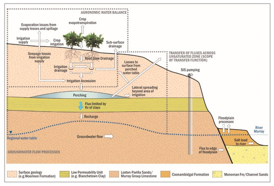
Figure 1.
Conceptualizations of the Loxton-Bookpurnong Irrigation District, showing perched water table under the irrigation district, and groundwater flow to the River Murray. model used to simulate recharge under perched water tables.
Figure 2 shows the conceptual model for the fluxes in the vadose zone. There are three semi-infinite layers of homogeneous soils, in which the second layer is of lower permeability. The left boundary condition is a no flow boundary, which means this is a line of symmetry. The upper boundary is the base of the agronomic zone, the left side of which underlies irrigated agriculture, and to the right side underlies non-irrigated agriculture. The upper boundary condition is a downward water flux, irrigation accession, as determined by agricultural practices, including channel leakage and spillage. For the one-dimensional systems discussed below, the whole upper surface is irrigated. The lower boundary condition is the water table, which is assumed to be constant. The profile is assumed to be initially at steady-state, with the root zone drainage at the boundary condition being relevant to either native vegetation or non-irrigated agriculture. At time zero, irrigation is implemented leading to an increase in root zone drainage. As the vertical flux may also consist of leakage or spillage from channels, it will be referred to as irrigation accession. In the western Murray Basin context, the new irrigation accession rate is ~100–400 mm/year), while the pre-irrigation flux (~0.1 mm/year for native vegetation or 2–30 mm/year for dryland agriculture).
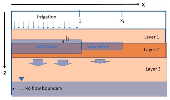
Figure 2.
Used to simulate recharge under perched water tables. The left-hand boundary is a no flow boundary, representing a line of symmetry. The variables are non-dimensionalised, with x = 1 being the outer limit of irrigation and x = x1 being the outer limit of perched water. Below layer 3 is the saturated zone of the aquifer.
This paper considers situations, where there is a reasonable probability of perched water tables under the irrigation area. This means that the irrigation accession should be sufficiently high or the saturated vertical conductivity sufficiently low for perched water tables to occur. Where it does occur, the ponded head builds up on the impeding layer and water moves laterally over the impeding layer, where it infiltrates into the impeding layer.
The layers of the unsaturated zone have been parameterised using the modified Mualem–Brooks–Corey model [21,22] for each layer. The water retention curve is given by:
where ψ is the soil suction, hb is the air-entry point, λ is a fitting parameter, and the relative saturation, , is given by
where θ is the volumetric water content, θr is the residual volumetric water content and θs is the saturation volumetric water content. The relative permeability, Kr, is given by:
where m is a fitting parameter related to the connectivity of soil pores.
Ɵ = (ψ/hb)−λ, ψ > hb
Θ = 1, ψ ≤ hb
Kr =Θm,
The hydraulic conductivity, K, is obtained by multiplying Kr by the saturated hydraulic conductivity. These parameters will be different for the different layers and a subscript i will be subsequently used to distinguish layer i. The parameters are assumed to be the same for both vertical and horizontal properties, except for the saturated conductivity. A superscript h and v will be used with the saturated hydraulic conductivity to characterise anisotropy. The values given to the parameters is given in the Methods section.
The underlying equations are non-dimensionalised using the vertical length scale, l2, timescale S2l2/Ks2v, horizontal length scale x0, and vertical flux Ks2v; where li is the thickness of the ith layer; x0 is the half-width of the irrigated area; Ksiv is the saturated vertical conductivity of the ith layer; and S2 is the specific yield for the 2nd layer for the initial dry conditions. The purpose of the non-dimensionalisation is to simplify the range of situations as much as possible using scaling and non-dimensional variables.
2.1. Unsaturated Zone Conditions
The PerTy3 model, as it relates to new developments, is adapted from the wetting front model [5]. In that model, the movement of water through the vadose zone occurs via gravity, causing a pressure (or wetting) front. Behind the wetting front, the flux of water is equal to the new flux, while below it, the flux equals the old flux. The wetting front moves with the speed (non-dimensional):
where zwf is the depth of the wetting front below the land surface; An and Ao are the non-dimensional irrigation accessions for the irrigated and pre-existing agriculture respectively; and θn and θo are the volumetric water contents above and below the wetting front. Their values are such that the relative vertical hydraulic conductivity equals An and Ao, respectively. When the pressure front reaches the water table, the recharge (dimensioned) increases from IAo to IAn. Equation (5) can be used to estimate the time delay between the change in land use and the change in groundwater recharge. The above theory, or variants of it, has been used to estimate time delays for changes in non-irrigated agriculture to affect the underlying groundwater. In this paper, we look to adapt this model to the situation, where the soil conductivity of parts of the vadose zone is sufficiently low to not allow the new water flux to move vertically by gravity alone. The simplicity of the model is appropriate for our knowledge of soil properties and input fluxes over representative scales. The parameters in Equations (1)–(4) will change for each layer. A subscript ‘i’ will be used to denote these parameters for layer i.
dzwf/dt = (An − Ao)/(θn − θo)
2.2. Situations Where Perched Water Tables Occur
The conceptual model in PerTy3 considers five stages for the pressure front to move through to the water table and for the new recharge rate to be attained. These are:
Stage 1: the pressure front moves through first layer according to Equation (5).
Stage 2: the interface between layers 1 and 2 needs to become saturated for the perched situation to occur. A wetting front continues to move through layer 2 while the moisture content about the interface is increasing. However, the dimensionless vertical flux across a broad zone from above the interface to below the pressure front is reducing from An to Ao.
Stage 3: saturated conditions develop at the interfaces of the first and second layers. This causes a saturation front to move downward behind the wetting front into layer 2, while the perched layer begins to build up in layer 1. The zone between wetting and saturation fronts is near-saturated and can be broad. The perched layer causes the hydraulic gradient in the saturated zone to be greater than that of gravity alone. As the ponded head rises, the hydraulic gradient continues to increase and the flux behind the wetting front increases. Water begins to move laterally above the interface between layers one and two and begins to infiltrate into the impeding layer.
Stage 4: the wetting front has reached the base of layer 2 and begins to move through layer three. The surface of the perched water table continues to rise towards an equilibrium, as does the flux behind the wetting front. As the flux increases, the saturation zone moves slowly towards the base of layer 2.
Stage 5: the wetting front has reached the water table. The recharge rises from the old irrigation accession rate. The recharge continues to rise until the perched water table reaches a new equilibrium. This occurs when the increased gradient through the second layer and the increased area of infiltration means that the recharge is equal to the irrigation accession. Where layer one is sufficiently thin, water from the perched water table is intercepted either by evapotranspiration or sub-surface drainage. This prevents the recharge from reaching the irrigation accession flux.
In adapting the wetting front model to perched situations, the following changes are incurred:
- Darcy’s Law is applied to the saturated zone in the upper clay layer. We assume that all of the hydraulic resistance is due to the clay and hence proportional to the thickness of the saturated layer, while the ponded head means a hydraulic gradient greater than one, purely due to gravity.
- The ponded head increases to the stage where the irrigation accession flux can pass through layer 2, or it fills all of layer 1.
- The perching results in a distribution of transit times for a change in irrigation accession rate to reach the water table.
- There may be a difference in magnitude between the irrigation accession and recharge, but only where some of the irrigation accession is returned to the land surface. If not, at equilibrium the recharge rate equals the irrigation accession rate.
- We have found it necessary to no longer consider the wetting front as a sharp transition from pre-development conditions to saturation. The existence of air-entry suction, below which hydraulic conditions the same as saturation occur and the near saturated zone means that the transition can be significant.
- As the wetting front moves through layer 3, the increasing vertical water flux at the base of layer 2 can lead to the wetting front moving more quickly as it moves to the water table.
The sections below describe these stages in more mathematical detail. Table 1 lists all the parameters used, their symbols and units and the equation number, where first used.

Table 1.
Glossary of parameters, symbols and units used in equations and the equation number, where first used.
2.3. Stage 1
During stage 1, the rate of movement of the wetting front is given by Equation (5). The dimensionless time for the wetting front to reach the top of the clay layer is given by:
t1 = l1(θn1 − θo1)/((An − Ao)l2)
The variable t1 is sensitive to θn1, this needs to be calculated for the new flux.
2.4. Stage 2
Once the wetting front reaches the interface between layers 1 and 2, the low permeability of layer 2 means that moisture begins to accumulate about the interface. The additional moisture creates a moisture gradient both below and above the interface in different directions. These gradients allow more or less moisture than would occur by gravity alone at that moisture content and allows the flux and soil suction to be continuous at the interface. A mass balance argument means that the difference in flux at the upper and lower ends of the segment is equal to the rate of accumulation in that segment. The time for saturation to occur is given by:
where θb is the background water content. For layer 1, this background value is the new moisture content and for layer 2, this is the old moisture content. We will return to the calculation of integral (7) later.
t2 = ∫(θ − θb)dz/(An − Ao),
2.5. Stage 3
The dimensionless equations describing the mass balance of the perched layer are:
where
h is the head of the perched water table, x = 1 represents the edge of the irrigation field; x = x1 is the edge of the wetted zone outside of the irrigation field; x0 is the half-width of the irrigated field; and q is the vertical flux into layer 2. Continuity in h and the flux of water (and therefore gradient in h) is assumed to occur at x = 1. At x = x1, h is zero.
B = Ks1hl22/(Ks2vx02)
A = IAn/Ks2v
β = (θs1 − θn1)/(θs2 − θo2)
For the above equations, A is a dimensionless parameter that reflects the degree of perching, with perching not occurring for smaller A and interception of the perched head with the upper boundary condition for larger A. The dimensionless parameter, B, reflects the degree to which lateral movement occurs. As B approaches zero, there is no lateral movement and the system behaves as a 1D system. For very large B, the perched layer spreads thinly across the impeding layer. We also shall assume for this stage, that the head of the perched layer is lower than the upper boundary, i.e.,
h ≤ l1/l2
Darcy’s Law across the saturated zone implies that:
where zsat is the depth of the saturation front. This assumes that the main hydraulic impedance is in the second layer. Under the wetting front model,
q = 1 + h/zsat
dzwf/dt = q
This assumes that the new flux is much greater than the old flux. During Stage 3, the wetting front has not reached the base of layer 2.
In addition to the equations above, some further assumptions are added in order to estimate recharge:
- We shall ignore the effect of the ponded head outside the irrigated field on the infiltration into the impeding layer, i.e.,
q = dzwf/dt = 1, 1 < x < x1
- 2.
- We shall assume quasi-steady-state Depuit–Forchheimer equations for this area, which leads to the following equations:
h = (1 + sqrt(B)h1 − x)/sqrt(B), 1 < x < x1
x1= h1sqrt(B) + 1, and
- 3.
- We shall assume that the head is constant across the irrigated field. Combining Equations (8), (9), (18) and (19) gives:
βdh1/dt = A − q − h1sqrt(B). 0< x < x1
- 4.
- We shall assume in early times of ponding that the lateral movement is small, and processes are vertical. We shall also assume that the separation between saturation fronts and wetting fronts is constant. By defining the dimensionless parameter:we find that zsat and h increase linearly:α = h/zsat,zsat = (1 + α)th = α(1 + α)tα = (−(1 + β) + sqrt((1 + β)2 + 4(A − 1)β)/(2β), andq = 1 + α
Equation (25) indicates a flux greater than the free drainage flux through a saturated clay layer (q = 1).
Stage 3 finishes when the wetting front reaches the bottom of layer 2. To estimate when this occurs, it is necessary to estimate the thickness of the zone, Φ, between the wetting front and the saturated zone (Figure 3a). If we assume that this zone is in a quasi-steady state, this can be estimated from Darcy equation to give:
where φ is a soil hydraulic property and the integral in Equation (26) goes from 0 (saturated) to ψ3, and in Equation (27) from hb2 to ψ3, where ψ3 is either (a) the matric potential relating to the pre-development drainage, where the transition zone is entirely within the clay layer or (b) the soil matric suction at the interface with layer 3. We shall assume that φ is constant with respect to q.
Φ = φ/(q − 1) = ∫dψ/((q/Kr(ψ) − 1)l2),
Φ = hb2/((q − 1)l2)+ ∫ dψ/((q/(Kr(ψ) − 1)l2)
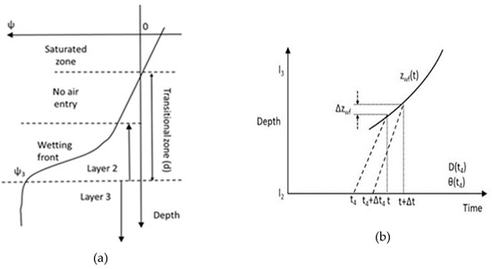
Figure 3.
Figures showing two aspects of the modelling: (a) near-saturated zone between wetting front and saturation front, as described in Equation (26); and (b) changing speed of wetting front, as flux behind increases.
Once the wetting front reaches the base of layer 2, the flux at top of layer 3 increases to q = 1 + α and the wetting front begins to move through this layer. This occurs at non-dimensional time after perching begins:
and the ponded head will be:
t3 = (1 − φ/α)/(1 + α),
ho = α − φ
By knowing the flux during this third stage, it is possible to use the steady-state Darcy’s Law to calculate t2 in Equation (7).
2.6. Stage 4
After the wetting front reaches the base of layer 2, Equations (14) and (26) can be combined to estimate the vertical flux:
q = h + 1 + φ
Incorporating Equation (30) into (20), the mass balance for the perched layer becomes:
where φ is calculated using Equation (27). This has the solution:
where h0 and t0 are, respectively, the head and time at which the wetting front breaks through the clay layer Equation (29). The equilibrium head, heq, is given by:
h = heq + exp(−(t − t0)(1 + sqrt(B))/β)(h0 − heq)
heq = (A − 1 − φ)/(1 + sqrt(B))
The effect of B is to not only reduce the steady-state ponded head, but it also quickens the rate at which it is attained. To understand this better, we consider the dimensioned time scale:
ts = l2S2β/((1 + sqrt(B))Ks2v)
As B becomes very large, ts becomes:
ts ~ x0s1/sqrt(Ks1h Ks2v)
Hence, the time scale involves a mixture of the horizontal conductivity of the sand layer and the vertical conductivity of the clay layer. This is not surprising given that both soil parameters influence both the magnitude of the ponded head and the ability of the water to move laterally.
Equation (30) implies that the vertical flux through the clay layer would also approach exponentially the equilibrium value qeq from q0. Equation (30) and Equation (32). The extent of the wetting outside the irrigation field also increases exponentially to the equilibrium value x1eq from x10 in parallel with the ponded head (Equation (18) and Equation (32)). Equation (16) implies that the aggregated vertical flux through the clay external to the irrigation field is proportional to the extent of wetting.
As the flux at the base of layer 2 increases, the velocity of the wetting front can increase. The speed of the wetting front is given by Equation (5), but with A replaced by q. Unlike the situation where there is no perching, the water content at the wetting front, θwf, is likely to change as the flux at the bottom of layer 2 changes gradually. The change in flux (and associated water content) will move at a speed determined by the group velocity, dK/dθ. This will continue until the change reaches either the wetting front or the capillary fringe (in the case, where the wetting front has already reached the capillary fringe). In the former situation, the time at which the change reaches the wetting front is given by:
where t4 is the time at which the change at the change occurs at the bottom of layer 2 and dK/dθ(θ(t4)) = vg is the group velocity as determined there.
t − t4 = zwf/(dK/dθ(θ(t0))) = zwf/vg,
Figure 3b shows the process of calculating the rate of movement of the wetting front. Following the logic of that diagram allows zwf to be calculated by integrating the following equation:
where vwf is the velocity of the wetting front and vg is the group velocity. If dK/dθ >> ΔK/Δθ, as is the case for our parameterisation of layer 3, this simplifies to:
Δzwf = vwfΔt4/(1 + vwf/vg)
zwf = ∫vwfdt4
Equation (38) implies that changes in flux and water content at the base of layer 2 are transmitted quickly to the wetting front. This causes the wetting front to move more quickly. Once the wetting front reaches the water table, the changes in flux should transmit quickly to the water table. Under the assumption that dK/dθ >> ΔK/Δθ, the gap in time between the flux at the base of layer 2 disappears. The effect of the higher fluxes at the base of layer 2 during the propagation of the wetting front through layer 3 is to quicken the pace of the wetting front but also to increase the flux at the time the wetting front reaches the water table. The speed at which the wetting front moves through layer 3 is less than that for the unperched situation as the flux at the base of layer 2 is less than for the unperched situation.
Computationally, the inclusion of the assumption simplifies and quickens the algorithms but not including the assumption is still computationally viable. The simpler assumption is made in PerTy3.
2.7. Stage 5
Once the wetting front reaches the water table, recharge rises from the pre-development flux to a new higher flux, less than the irrigation flux. The recharge rate continues to increase, exponentially asymptoting to the irrigation accession flux. The program ignores the effect of capillary fringe on timing. For example, for native vegetation or dryland agriculture the corresponding soil suction could be up to 10 m, while for irrigated agriculture, the corresponding suction is more likely 10′s of cm. We shall assume that the bottom of layer 3 is the capillary fringe corresponding to irrigation.
If the perched head rises to the stage where it intercepts the upper boundary condition, there is no capacity for further infiltration to occur. We refer to this as recharge rejection. This occurs when:
heq = (A − 1 − φ)/(1 + sqrt(B)), h > l1/l2
Any excess water is returned to the surface as evapotranspiration. This process can lead to waterlogging and salinity and generally sub-surface drainage is required. The volume of rejected recharge can be estimated using Equations (19) and (30):
D/IA = (A − 1 − φ − h(1 + sqrt(B)))/A
In portraying outputs, a normalised transfer function is often used:
TF(t) = (R(t) − Ro)/(IAn − IAo)
A transfer function is a mathematical model of a system that maps its input to its output (or response). An analogous transfer function can be defined for drainage (or rejected recharge). Where there is no rejected recharge, TF(t) = 0 for t = 0; and approaches 1 after long periods. Hence it represents a cumulative probability distribution for time delays for pressure to travel through the vadose zone. Where there is rejected recharge, TF(t) is less than one after long periods but the sum of transfer functions for recharge and drainage approaches one. Transfer functions take on greater significance where they can be superimposed for a combination of actions. A modified transfer function will be defined below for application to superposition.
2.8. Theory: Summary
- Irrigation development leads to the formation of a wetting front that moves through layer 1.
- Once the wetting front reaches the interface between layers 1 and 2, the low permeability of layer 2 means that moisture begins to accumulate about the interface.
- The ponded head is zero until the end of Stage 2, increases linearly until end of stage 3 and then exponentially asymptotes to an equilibrium head during stages 4 and 5.
- The flux at the base of layer 2 is zero until the end of stage 3 and then increases exponentially to the irrigation accession rate.
- The recharge rate is zero until the end of stage 4 and then increases exponentially to the irrigation accession flux.
- While the ponded head increases to the stage where the irrigation accession flux passes through layer 2, the value of this may be so high that it intercepts the upper surface.
3. Methods
This section describes the modelling methodology used to meet objectives 1 and 2(a–b) of the study; namely to benchmark the PerTy3 model against an appropriate numerical model; develop a process for estimating recharge under brownfield developments; and explore the use of even simpler modelling approaches based upon superposition of actions, and conceptual approximants for transfer functions.
3.1. Model Implementation
To achieve these objectives, a series of implementations of the PerTy3 and the numerical model, FEFLOW (finite-element subsurface flow simulation system), are used. The default parameters used for both the one- and two-dimensional (2D) modelling are shown in Table 2. One-dimensional (1D) situations represents those, where lateral movement of water is minimal, and hence where B approximates zero. The default parameters have been derived using published estimates of soil hydraulic parameters for the Mallee region [23] and defining equivalent parameters for the Brooks–Corey–Mualem model. The irrigation flux pre-development, IAo, has been assumed to be 10 mm/year for all experiments. For the two-dimensional experiments, the half-width of the irrigation area is assumed to be 500 m. Pertinent information on the irrigation water balance is from [24].
Table 2.
Default soil parameters used in the modelling.
The numerical modelling is undertaken using FEFLOWTM [25]. FEFLOW solves the governing flow equations in porous media for variable saturation. Richards’ equation is solved for a single dominant fluid phase (in this case water) with an assumed stagnant air phase that is at atmospheric pressure everywhere. FEFLOW implements a number of empirical and spline models for variable saturation. Fine mesh refinement is used to achieve stable numerical solutions for the adopted choices of the Mualem–Brooks–Corey model parameters. The vertical mesh size for both the 1D and 2D modelling is 10 cm (250 (1D) or 150 (2D) elements), while for the 2D modelling, the horizontal mesh size is 10 m (200 elements).
Table 3 details the various modelling experiments and the associated parameters. The modelling has been designed to achieve the various objectives:
Table 3.
Benchmarking experiments.
- 1–6 (1D), 1–4 (2D) are a series of simulations for new developments that cover a range of non-perched and perched situations and illustrate varying degrees of lateral movement. These simulations demonstrate the main processes and the outputs allow benchmarking of the models. For each experiment, the PerTy3 and FEFLOW models are used.
- The experiments 5–10 (2D) are designed, in conjunction with Experiments 1–4 (2D), to explore the effect of a brownfield developments in the vicinity of a development, already at equilibrium. More specifically, the recharge under a greenfield development (1–4(2D)) is compared to brownfield developments either directly adjacent to or 250 m away from a development at equilibrium. The FEFLOW outputs will be compared to the superposition of the two developments.
- Experiments 10–13 (2D) are designed to compare recharge brownfield sites in the vicinity of greenfield sites, that are 5 years old. The FEFLOW outputs will be compared to the superposition of the two developments.
3.2. Transfer Functions and Superposition
In this section, we describe the concept of a transfer function for application to superposition, to support objective 2(a). For this purpose, a modified transfer function for the recharge is defined:
where the superscript * indicates the minimum of IA and the maximum irrigation accession without rejected recharge. We can define a similar transfer function for drainage, TF″, where:
where Do is the original drainage rate, IA** is the maximum of IA and the maximum irrigation accession that occurs without rejected recharge.
TF′(t) = (R(t) − Ro)/(IAn* − IAo*)
TF″(t) = (D(t) − Do)/(IAn** − IAo**)
The general aim is to generate outputs, with appropriate accuracy, for a range of inputs. In line with information theory, we would look to see whether simplifications are possible, by using, for example, processes, such as superposition. As the system is not necessarily linear, there is no reason to believe that superposition would necessarily apply to a range of situations. Some situations are not expected to follow superposition including those where thresholds are involved, such as the initiation of perching or rejected recharge. The addition of two actions, that do not individually exceed the threshold but in aggregation do so, is not linear.
If superposition does apply, the aggregate transfer function for a sequence of actions that affect irrigation accession:
where IAj is a sequence of modified irrigation accessions that occur from j = 0 to j = p + 1 and TF’j+1 is the modified transfer function that applies for a change of irrigation accession from IA*j to IA*j+1.
TF’(t) = (∑j(IA*j+1 − IA*j) TF’j+1)/(IA*p+1 − IA*0)
The pattern of the aggregate TF’ with time would broadly follow that of IA, perhaps with time delays and some ‘smearing’ and capping at the maximum irrigation accession for which there is no rejected recharge. Where superposition applies, this could simplify the numerical process. The transfer function could be generated for individual actions alone and this allows the overall aggregated transfer function to be generated. While the theory above describes physical processes, the analytical model is simplified, with assumptions such as spatial homogeneity, flat surface elevations etc. It is possible to consider transfer functions as conceptual models, using enough complexity to broadly replicate the recharge response. Such models have previously been used for recharge [16,18].
For this paper, we will compare the recharge under a brownfield development and the original greenfield development with the superposition of the two individual recharge outputs. Brownfield sites were thought previously to have shorter time delays, as they have already been wetted. Should the superposition be a good approximation, this may simplify the estimation of recharge under a complex irrigation district by allowing each development to be considered individually and then aggregated.
3.3. Approximants
In this section, we explore the application of approximants for the transfer function. In general, an approximant is a function, series, or other expression which is an approximation to the solution of a problem. Here, we trial the application of a conceptual model, specifically a linear reservoir model with a time delay, to approximate transfer functions, namely:
where a, t5 and t6 are fitted parameters. Such models have previously been used [18] for recharge through a deep vadose zone. Such conceptual models have been used widely in surface hydrology to calibrate surface flow models. The linear reservoir model forms a good approximation where the output (recharge) is a linear function of the storage (the mass of water in the unsaturated zone) [18].
TF(t) ~ 1 − exp(−a(t − t6)), t > t5
4. Results
4.1. One-Dimensional Modelling
Figure 4a compares the outputs for FEFLOW and PerTy3 for transfer functions for modelling Experiments 1(1D)–6(1D). There was no perching for Experiments 1, 2 and 5. These resemble step-functions, with consistency of results between the two forms of modelling. The values of A for these experiments were 0.3, 0.75 and 0.75, respectively. The model outputs were again consistent, with Experiments 3 and 6 showing perching. The transfer function showed a step increase, followed by an apparent exponential approach to one. The model outputs for the ponded head for these experiments are also consistent (Figure 4b) and both show an exponential approach to equilibrium after a delay and an initial linear rise. The values of A for these experiments were both 1.5. The modelling outputs for Experiment 4 show the least consistency with the numerical rise in the transfer function being slower; and the ponded rise occurring slightly later but both intercepting the upper surface (500 cm). Drainage or rejected recharge occurs with the increase for the analytical function occurring nearly 5 years later than the numerical output for drainage. Overall, the modelling outputs show that the processes are correct and the outputs are adequate for use in groundwater modelling.
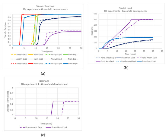
Figure 4.
Of outputs from one-dimensional outputs from PerTy3 (semi-analyt-ical) (dashed) and FEFLOW (numerical) (solid) models (a) transfer functions; (b) ponded head and (c) normalized drainage volume.
4.2. Two-Dimensional Modelling
The outputs for both the FEFLOW and PerTy3 models are consistent across a range of values of B from 0.1 to 10 (Figure 5a). The PerTy3 outputs are flatter and lower than those from FEFLOW. This is due to the representation of recharge external to the irrigated field (Figure 5b). The partitioning between recharge occurring outside and inside the irrigated field is consistent across the models, but PerTy3 shows initial delays in recharge occurring outside the field. Another modelling experiment (not shown here) shows even greater inconsistency, suggesting that assumptions were not adequate. The most likely cause is the lack of consideration of ponding external to the irrigated field. This would have the effect of delaying recharge increases.
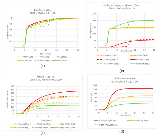
Figure 5.
Comparison of outputs from two-dimensional semi-analytical and numerical modelling for new accession rate of 200 mm/year: (a) Transfer functions (Total) for B = 0.1, 1, 10; (b) Transfer functions (total, under irrigation field, external to irrigation field) for B = 10. (c) Perched heads for B = 0.1, 1.0, 10 for an increase in IA to 200 mm/year. The head for the FEFLOW model is for x = 0, while that for PerTy3 is an average across the irrigated field. (d) the width of the wetted zone outside the irrigation field for B = 0.1, 1.0, 10, and an increase in IA to 200 mm/year.
The FEFLOW output for the perched head (Figure 5c) if for x = 0, while that for PerTy3 is an average across the irrigation field. While the FEFLOW output is higher than the PerTy3, the temporal distributions are approximately parallel. There is a large change in head for B = 0.1 (340 cm) to B = 10 (120 cm). The wetted width PerTy3 outputs (Figure 5d) shows a large variation from 90 m (B = 0.1) to 250 m (B = 10).
4.3. Modelling of Brownfield Developments
The effect of brownfield developments at a range of distances is shown in Figure 6. For low values of B (Figure 6a), there is almost no difference whether the new development is placed next to an existing field or at infinite distance (greenfield development). Even for B of 10, there is not much difference. For brownfield developments next to an existing development at equilibrium (Figure 6b), there is some earlier recharge and then later some delayed recharge. The earlier recharge is presumably due to pre-wetting by the existing development and the later delays due to the expansion on one side being constrained by the existing development.
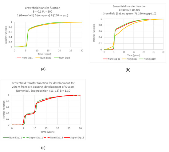
Figure 6.
Functions for brownfield developments: (a) numerical outputs at varying distances from a pre-existing steady-state development and B = 0.1; (b) numerical outputs at varying distances from a pre-existing steady-state development and B = 10; (c) numerical outputs for the total development of a new development followed by another development, 250 m away for B = 1, 10 compared to superposition of numerical outputs for two independent developments, one 5 years after the other.
For brownfield developments occurring 5 years after a new development (Figure 6c) there is, minimal effect of separation.
4.4. Approximants
The trial of approximants was mostly successful with good matching with an exponential function (Figure 7). The worst fit was for Experiment 4 (1D) (Figure 7a). For this experiment, the ponded head reached the upper boundary condition by about year 17. This appears to change the temporal pattern of recharge, which is not captured by the approximant.
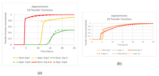
Figure 7.
Approximants against numerical solutions for which perching occurs. Solid lines represent numerical solutions and dashed lines approximants. (a) 1D modelling experiments 3, 4 and 6. The approximants are respectively: 1 − exp(− 0.07 × (t + 10)), t < 12; 4: min(0.486,1 − exp(−0.18 × (t − 14))), t > 15; and 6: 1 − exp( − 0.22 × (t + 4.4)), t > 5. (b) 2D Modelling Experiments 2, 3 and 3a. The approximants are respectively: 2: 1 − exp(− 0.12 × (t + 2.5)), t > 6; 3: 1 − exp( − 0.13 × (t − 0.8)), t > 4; and 3a:1 − exp(−0.15 × (t + 1)), t > 5.
The coefficient in the exponential is similar for all the 2D modelling experiments. The theory is predicting change in the exponential for experiment 3a. On the other hand, the 1D modelling is showing considerable variation, which was not expected. However, Figure 4a shows that the analytical expressions, which have similar coefficients for all the experiments, adequately fit the numerical simulation. The 1D modelling is trying to fit over small variations of the transfer function and then becomes sensitive to issues such as numerical dispersion.
Perhaps the largest difficulties are 1) the estimation of the time delay until recharge occurs and 2) the reference time in the exponential. However, the analytical model appears to be adequately estimating time delays and becomes an issue of finding the simplest form of estimation.
Overall, the collection of results shows promise for using approximants, in addition to using a PerTy3 or numerical models.
5. Discussion
5.1. Accuracy of Modelling
Modelling will necessarily involve simplifications of reality. For example, (1) all surfaces are assumed to be topographically flat; and (2) layers are considered to be physically homogeneous with known properties. The values of hydraulic properties need to be considered to be conceptual in nature, rather than being true values. The study here has tried to incorporate the key processes. The comparison between models tests mathematical errors.
The comparison of model outputs show that the outputs were consistent in most aspects for the 1D modelling. Two exceptions were (1) the transfer function for Experiment 4; the situation involving interception of the ponded head with the upper boundary condition; and (2) the drainage volumes for Experiment 4. These discrepancies were related in that the PerTy3 output showed that the perched head reached the upper boundary condition about five years later than the FEFLOW output. This has led to drainage volumes occurring five years later, although volumes were similar. It also meant that recharge has equilibrated at about the same time as this interception for PerTy3; while recharge has equilibrated some years after the perched head has intercepted the upper surface, causing a distortion of the transfer function. Despite these discrepancies, the consistency of the model shows that the representation of the processes are accurate.
The comparison of model outputs for 2D modelling does not show the same level of consistency. In particular, PerTy3, compared to FEFLOW, overpredicts (1) the delay in recharge occurring external to the irrigated field; and (2) the exponential decay in transfer function. Both may be due to ignoring the additional ponded head on recharge external to the irrigated field. The mound extends beyond the irrigated field [24] and this reduces delays for recharge to occur, causing recharge to increase continuously rather than be delayed. The mounding also changes the shape of the moisture storage in the unsaturated zone, which will affect the exponential decay [19].
The outputs for FEFLOW and PerTy3 2D models are consistent in the partitioning of recharge between under the irrigated field and external to the irrigated field; the reduction of the perched head with B, and the exponential decay of perched head and wetted width. Thus, while some 2-dimensional aspects are not adequately modelled, most other aspects appear to be adequate for the objectives of the transfer function.
The comparison of model outputs with field observations will be discussed in [20].
5.2. Brownfield Developments
There has been some discussion in the Australian context, that brownfield developments should respond more quickly due to antecedent moisture. The results here show that while this partially occurs for high values for B, there are no lateral impacts (i) for B = 0.1 or 1, or (ii) for separations of 250 m or more; and that (iii) for no separation, there are delays in recharge that outweigh the early breakthroughs. The lack of lateral impacts, especially for B = 0.1, 1, appears to be due to limited wetted extent outside irrigated fields. The later time delays for B = 10 are probably due to the inability of water to move laterally on one side. The effect would be similar to a larger irrigation field, with higher perched water table and relatively smaller wetted extent.
The small interaction between irrigated fields means that a complex irrigation area with new developments occurring at different times could be modelled as a superposition of impacts for individual fields. This would greatly simplify the calculation of recharge under the irrigation district. Should the circumstances be such that there are interactions (high B, small gaps between irrigation fields, the results here indicate that there may be simple approximations, but this would require more work.
5.3. Approximants
The study showed that the transfer functions for both 1D and 2D were able to be approximated by an exponential function with a reference time. The best-fit coefficient for the exponential was consistent across the 2D modelling, but variable for the 1D modelling. However, the analytical value was reasonable for five of the six 1D outputs, suggesting that one value may be a reasonable approximation for most situations. If so, this requires only for the reference time and the time delay (the time at which recharge, and the exponential approximation begins). This was not investigated in this study. However, PerTy3 appears to be able to estimate the time delay and the change in recharge at that time, so it may become a matter of finding how this could be simplified or how these parameters change in response to different model parameters. The exponential function can be derived from a linear reservoir model in which the total recharge is linear with respect to the mass of water in the perched water table.
The use of approximants and superposition may lead to simplification of the estimation of recharge. The approximants form a step towards considering transfer functions as conceptual models that are fitted by the groundwater response. This has been done previously [16,18] for situations where response times are quicker and individual events are independent. These are then used for calibration. For the situations considered here, the response from different actions gradually accumulate into one single evolving groundwater response. This can be used to calibrate the transfer function, where there is no rejected recharge and provided transfer functions do not vary greatly for different actions. Where there is rejected recharge, drainage can be used for calibration.
5.4. Data Requirements
Superficially, the model appears to require many parameters and hence should be considered as complex. For example, the model, in principle, requires several soil parameters for each layer. However, many of these parameters are based on texture and can be approximated based on lithology information and data [23]. The saturated vertical hydraulic conductivity for layer 2 and horizontal conductivity for layer 1 appear to be critical parameters and are reflected in the dimensionless variables A and B, which portray the range of behavior expected in the field [19]. A critical input to the model is the irrigation accession, IA. This also is incorporated in the dimensionless variable A. Where district-scale flux data is used e.g., surface water diversions, length of channels, this can only be converted to IA through a good knowledge of the irrigation area and how it has changed over the history of the irrigation district. In some cases, agronomic experiments have been conducted to estimate the field water balance and hence water-use efficiency factors. Information of this type may be able to highlight how irrigation accessions have changed over time in response to changed technology, rainfall and availability of surface water. While PerTy3 has not represented this component of the water balance, its accuracy is dependent on good information on surface water balance. The need for drainage is a sign that there is rejected recharge and is useful for the calibration of soil hydraulic parameters [19].
5.5. Further Work
The work above has shown that the processes are well understood; that the 1D modelling of these processes appears to be adequate, but the 2D modelling is only adequate for some aspects. In particular, the assumption that the ponded head is effectively zero external to the irrigated field is clearly inadequate. Some improvement to the model are, therefore, required, perhaps by considering the quasi-steady state analytical models [26], in which a non-zero perched head is incorporated. The 2D transfer function does not vary significantly from the 1D modelling, suggesting that the one transfer function may be adequate for a wide range of situations, and that an exponential model appears to be an adequate approximation. This suggests that such approximants may be useful for estimating recharge, but this requires more work. Brownfield irrigation developments appear to only differ from greenfield developments for large B parameters and for separations of less than 250 m. This suggests that treating developments as independent may be a reasonable approximation of a range of situations. However, more work would be required for the other situations to find the best estimation method.
6. Conclusions
This paper has described the modelling of recharge from new irrigation developments, where there is the potential for perching over a deep vadose zone. The model relies on a surface water balance of the irrigation area and is intended to provide input to regional groundwater models. The model adapts algorithms for which there is no perching to those with perching, allowing a smooth transition through the parameter A.
The work shows that hydrological equilibrium between irrigation accession inputs and recharge to the water table can occur by increased hydraulic gradient through the clay and a greater area of ponded infiltration through the clay. Where the head of the perched water table is sufficiently close to the land surface, some water is returned to the land surface either through sub-surface drainage or by evapotranspiration. There is good agreement between estimates of recharge, ponded head and return to the surface from the semi-analytical PerTy3 model and those from the numerical FEFLOW model for one-dimensional situations, where recharge occurs beneath the irrigated fields. The perching leads to some proportion of the recharge occurring after a long time delay from the timing of the new development.
The model shows that for the parameter range chosen here the effect of two-dimensionality on the total recharge appears to be minor, whereas more detailed processes, such as the proportion of recharge that occurs external to the irrigation field and the ponded head, are sensitive. These latter lateral effects scale in a predictable fashion to a parameter B. Since recharge models usually only require the total recharge, the lack of sensitivity should simplify the modelling.
The modelling also shows that the recharge under brownfield developments, which are developed near pre-existing developments do not appear to be significantly different to that from greenfield developments. This allows the recharge under realistic and complex scenarios of irrigation development to be treated through superposition of recharge from individual fields.
The main input to PerTy3 is the irrigation accession under irrigation. The accuracy of the recharge outputs from PerTy3 is dependent on good information for irrigation accessions over the history of the irrigation development. This, in turn, is dependent on knowing how the irrigation area, and water-use efficiency has changed over time.
Author Contributions
Conceptualization, G.R.W., D.C. and T.S.; methodology, G.R.W., T.S.; software, G.R.W., T.S.; validation, G.R.W. and T.S.; formal analysis, G.R.W.; investigation, G.R.W. and T.S.; resources, D.C., G.R.W.; data curation, G.R.W., T.S. and D.C.; writing—original draft preparation, G.R.W. writing—review and editing, D.C.; project administration, D.C.; funding acquisition, D.C. All authors have read and agreed to the published version of the manuscript.
Funding
This research was partially funded by MURRAY-DARLING BASIN AUTHORITY, project number MD004683.
Acknowledgments
The authors would like to thank the members of the Technical Committee (Juliette Woods, Ray Evans, Emmanuel Xevi and Prathapar) and Hugh Middlemis for technical advice.
Conflicts of Interest
The authors declare no conflict of interest.
References
- Kurtzman, D.; Scanlon, B.R. Groundwater Recharge through Verti sols: Irrigated Cropland vs. Natural Land, Israel. Vadose Zone J. 2011, 10, 662–674. [Google Scholar] [CrossRef]
- Khan, S. Rethinking rational solutions for irrigation salinity. Australas. J. Water Resour. 2005, 9, 129–140. [Google Scholar] [CrossRef]
- Williams, J.; Grafton, R.Q. Missing in action: Possible effects of water recovery on stream and river flows in the Murray-Darling Basin, Australia. Australas. J. Water Resour. 2019, 23, 78–87. [Google Scholar] [CrossRef]
- Cook, P.G.; Jolly, I.D.; Walker, G.R.; Robinson, N.I. From drainage to recharge to discharge: Some timelags in subsurface hydrology. Dev. Water Sci. 2003, 50, 319–326. [Google Scholar] [CrossRef]
- Jolly, I.D.; Cook, P.G.; Allison, G.B.; Hughes, M.W. Simultaneous water and solute movement through unsaturated soil following an increase in recharge. J. Hydrol. 1989, 111, 391–396. [Google Scholar] [CrossRef]
- Rossman, N.R.; Zlotnik, V.A.; Rowe, C.M.; Szilagyi, J. Vadose zone lag time and potential 21st century climate change effects on spatially distributed groundwater recharge in the semi-arid Nebraska Sand Hills. J. Hydrol. 2014, 519, 656–669. [Google Scholar] [CrossRef]
- Bouwer, H. Effect of Irrigated Agriculture on Groundwater. J. Irrig. Drain. Eng. 1987, 113, 4–15. [Google Scholar] [CrossRef]
- Orr, B.R. A Transient Numerical Simulation of Perched Groundwater Flow at the Test Reactor Area, Idaho National Engineering and Environmental Laboratory, Idaho, 1952–1994; U.S. Geological Survey Water Resources Investigations Report 99-4277; U.S. Geological Survey: Denver, CO, USA, 1999.
- Truex, M.J.; Oostrom, M.; Carroll, K.C.; Chronister, G.B. Perched-Water Evaluation for the Deep Vadose Zone Beneath the B, BX, and BY Tank Farms Area of the Hanford Site; Pacific Northwest National Laboratory: Richland, WA, USA, 2013. [Google Scholar]
- Oostrom, M.; Truex, M.J.; Carroll, K.C.; Chronister, G.B. Perched-water analysis related to deep vadose zone contaminant transport and impact to groundwater. J. Hydrol. 2013, 505, 228–239. [Google Scholar] [CrossRef]
- Weiss, M.; Gvirtzman, H. Estimating Ground Water Recharge using Flow Models of Perched Karstic Aquifers. Groundwater 2007, 45, 761–773. [Google Scholar] [CrossRef] [PubMed]
- Ganot, Y.; Holtzman, R.; Weisbrod, N.; Nitzan, I.; Katz, Y.; Kurtzman, D. Monitoring and modeling infiltration-recharge dynamics of managed aquifer recharge with desalinated seawater. Hydrol. Earth Syst. Sci. 2017, 21, 4479–4493. [Google Scholar] [CrossRef]
- Rains, M.C.; Fogg, G.E.; Harte, T.; Dahlgren, R.A.; Williamson, R.J. The role of perched aquifers in hydrological connectivity and biogeochemical processes in vernal pool landscapes, Central Valley, California. J. Hydrol. 2013, 505, 228–239. [Google Scholar]
- Villeneuve, S.; Cook, P.G.; Shanafield, M.; Wood, C.; White, N. Groundwater recharge via infiltration through an ephemeral riverbed, central Australia. J. Arid Environ. 2015, 117, 47–58. [Google Scholar] [CrossRef]
- Murray-Darling Basin Authority. Basin Salinity Management 2030 (BSM2030). Murray-Darling Basin, Canberra. 2015. Available online: https://www.mdba.gov.au/publications/mdba-reports/basin-salinity-management-2030 (accessed on 26 March 2020).
- Besbes, M.; de Marsily, G. From infiltration to recharge: Use of a parametric transfer function. J. Hydrol. 1984, 74, 271–293. [Google Scholar] [CrossRef]
- Mattern, S.; Vanclooster, M. Estimating travel time of recharge water through a deep vadose zone using a transfer function model. Environ. Fluid Mech. 2010, 10, 121–135. [Google Scholar] [CrossRef]
- Wang, X.S.; Ma, M.-G.; Li, X.; Zhao, J.; Dong, P.; Zhou, J. Groundwater response to leakage of surface water through a thick vadose zone in the middle reaches area of Heihe River Basin, in China. Hydrol. Earth Syst. Sci. 2010, 14, 639–650. [Google Scholar] [CrossRef]
- Walker, G.R.; Currie, D.; Smith, A. Modelling the effect of efficiency measures and increased irrigation development on groundwater recharge through a deep vadose zone. Water. under review.
- Currie, D.; Laattoe, T.; Walker, G.R.; Smith, A.; Woods, J.; Bushaway, K. Modelling groundwater returns to streams from irrigation areas with perched water tables. Water. under review.
- Schaap, M.G.; van Genuchten, M.T. A Modified Mualem-van Genuchten Formulation for Improved Description of the Hydraulic Conductivity Near Saturation. Vadose Zone J. 2006, 5, 27–34. [Google Scholar] [CrossRef]
- Brooks, R.H.; Corey, A.T. Hydraulic Properties of Porous Media; Colorado State University: Fort Collins, CO, USA, 1964. [Google Scholar]
- Meissner, T. Relationship between soil properties of Mallee soils and parameters of two moisture characteristics models. In Proceedings of the SuperSoil 2004: 3rd Australian and New Zealand Soils Conference, Sydney, Australia, 5–9 December 2004; Available online: http://www.regional.org.au/au/pdf/asssi/supersoil2004/2018_meissnert.pdf (accessed on 26 March 2020).
- Meissner, T. Estimation of Accession for Loxton and Bookpurnong Irrigation Areas; Department of Environment and Water: Adelaide, Australia, 2019.
- Diersch, H.-J. Finite Element Modeling of Flow, Mass and Heat Transport in Porous and Fractured Media; Springer: Berlin/Heidelberg, Germany, 2014. [Google Scholar] [CrossRef]
- Kacimov, A.R.; Obnosov, Y.V. An exact analytical solution for steady seepage from a perched Aquifer to a low-permeable sublayer: Kirkham-Brock’s legacy revisited. Water Resour. Res. 2015, 51, 3093–3107. [Google Scholar] [CrossRef]
© 2020 by the authors. Licensee MDPI, Basel, Switzerland. This article is an open access article distributed under the terms and conditions of the Creative Commons Attribution (CC BY) license (http://creativecommons.org/licenses/by/4.0/).