Article

Recovery of Soil Hydraulic Properties for Assisted Passive and Active Restoration: Assessing Historical Land Use and Forest Structure

1
Laboratory of Ecology and Forest Restoration (LERF), Department of Biological Sciences, “Luiz de Queiroz” College of Agriculture, University of São Paulo, Av. Pádua Dias 11, Piracicaba SP 13418-900, Brazil
2
Department of Soil Science, “Luiz de Queiroz” College of Agriculture, University of São Paulo, Av. Pádua Dias 11, Piracicaba SP 13418-900, Brazil
3
Forest Hydrology Laboratory, “Luiz de Queiroz” College of Agriculture, University of São Paulo, Av. Pádua Dias 11, Piracicaba SP 13418-900, Brazil
4
Council for Agricultural Research and Economics, Research Centre for Agriculture and Environment (CREA-AA), Via C. Ulpiani 5, 70125 Bari, Italy
5
Université de Lyon, UMR5023 Ecologie des Hydrosystèmes Naturels et Anthropisés, CNRS, ENTPE, Université Lyon 1, 3 rue Maurice Audin, 69518 Vaulx-en-Velin, France
*
Author to whom correspondence should be addressed.
Water 2019, 11(1), 86; https://doi.org/10.3390/w11010086
Submission received: 22 November 2018 / Revised: 26 December 2018 / Accepted: 28 December 2018 / Published: 7 January 2019
(This article belongs to the Special Issue Soil Hydrology for a Sustainable Land Management: Theory and Practice)

Abstract

:
Tree planting and natural regeneration are the main approaches to achieve global forest restoration targets, affecting multiple hydrological processes, such as infiltration of rainfall. Our understanding of the effect of land use history and vegetation on the recovery of water infiltration and soil attributes in both restoration strategies is limited. Therefore, we investigated the recovery of top-soil saturated soil hydraulic conductivity (Ks), soil physical and hydraulic properties in five land use types: (i) a secondary old-growth forest; (ii) a forest established through assisted passive restoration 11 years ago; (iii) an actively restored forest, with a more intensive land use history and 11 years of age; (iv) a pasture with low-intensity use; and (v) a pasture with high-intensity use, in the Brazilian Atlantic Forest. For these land use types, we determined the historical land use patterns and conducted soil sampling, using the Beerkan method to determine Ks values in the field. We also measured tree basal area, canopy cover, vegetation height, tree density and species richness in forest covers. The Ks decreased when land use was more intense prior to forest restoration actions. Our results indicate that land use legacy is a crucial factor to explain the current difference in soil and vegetation attributes among study sites.

1. Introduction

Forest restoration strategies are being implemented around the world through ambitious international (e.g., Bonne Challenge and New York Declaration on Forests), regional (e.g., Initiative 20 × 20 and AFR100) and national initiatives such as restoration plans in many countries [1]. Consequently, secondary forests have expanded in tropical regions [1,2]. In Brazil, the location of our study area, the “Atlantic Forest Restoration Pact” aims by 2050 to increase the current forest cover from 17% to at least 30%, with a restoration target of 15 million hectares [3]. These initiatives include both passive and active restoration strategies. Passive ecological restoration refers to spontaneous recovery of tree species in an ecosystem that has been damaged, while assisted passive restoration involves human interventions to assist natural regeneration [4,5]. This can include introduction of propagules and removal of invasive species and persistent disturbances, for example, fire or livestock grazing [4]. On the other hand, active restoration requires a higher human intervention through planting of tree seedlings to accelerate the recovery process [6,7].
Both restoration approaches have been shown to impact positively the provision of ecosystem services, as well recovering biodiversity and ecosystem functions [8]. However, most restoration research around the world has focused on aboveground plant communities, whilst the belowground environment (e.g., soil physical and hydraulic properties) has been poorly studied [9,10]. For example, the response of the infiltration process, and soil physical and hydraulic properties after forest restoration is virtually unknown [11]. A crucial parameter in the infiltration process is the soil saturated hydraulic conductivity (Ks), which influences water percolation through the soil matrix [12,13]. It is well known from previous studies that Ks is highly variable compared to other soil physical properties [14,15]. In fact, the Ks depends strongly on the highly variable soil structure, and it is known to vary several orders of magnitude [16,17], especially on forested soils [18,19]. In general, Ks recovery and soil hydraulic properties have been reported separately in passive [20,21,22,23,24] and active [25,26,27,28] restoration, but few comparisons between both restoration strategies have been conducted. Lozano-Baez et al. [28] investigated the surface Ks recovery under a nine-year-old actively restored forest in the Atlantic Forest of Brazil and observed that the land use prior to forest restoration influences the Ks recovery. Moreover, the few recent comparisons between active and passive restoration show contradictory results. For instance, Ks at 12.5 cm depth in Brazilian Amazônia was higher under a 15-year-old passively restored forest than a 10-year-old tree plantation [11]. In contrast, other authors in Madagascar found much lower surface Ks in 2–10-year-old naturally regenerating fallow than actively restored forest of 6–9 years of age [29].
Most previous studies have assessed the recovery of soil physical and hydraulic properties without addressing the relationships among soil, vegetation and land use history. These relationships are fundamental to better understand the recovery process (e.g., resilience of the ecosystem) and successional trajectories after forest restoration [30,31]. Foster et al. [32] argued that the imprints of past land use on ecosystems may persist for decades to centuries. In particular, after forest restoration, such imprints of past land use on soil (e.g., Ks, soil physical and hydraulic properties) may persist for a time frame of more than a decade, as suggested by several studies [12,26,33]. However, the above-mentioned mechanisms and relationships that affect the recovery process are poorly understood.
As part of a larger research effort investing the effects of forest restoration on Ks, this study aimed to extend the work of Lozano-Baez et al. [28] at a new location. Apart from presenting new Ks data for pastures with different land use intensities and a secondary old-growth forest, this paper includes the first measurements of Ks for a forest established through assisted passive restoration in the Brazilian Atlantic Forest. We further quantified and compared the Ks, soil physical and hydraulic properties recovery of active vs. assisted passive restoration strategies from the same restoration program described by Lozano-Baez et al. [28]. We examined whether differences in land use history led to differences in these soil attributes (e.g., Ks, bulk density, soil organic carbon content, soil porosity, initial and saturated soil water content) and vegetation attributes (e.g., basal area, canopy cover, vegetation height, tree density and species richness). We studied five land-cover types: (i) a secondary old-growth forest, used as a reference forest (hereafter, RF); (ii) a forest established through assisted passive restoration (hereafter, APR); (iii) an actively restored forest (hereafter, AR); (iv) a pasture with low-intensity use (hereafter, LiP); and (v) a pasture with high-intensity use (hereafter, HiP). In forest stands, we associated the recovery of Ks, soil physical and hydraulic properties with the vegetation attributes. We hypothesized that Ks would vary with intensity of land use in the past among land-cover types as follows: RF > APR > AR > LiP > HiP. As the AR site had a more intensive land use history, we expected that Ks recovery and vegetation attributes would be higher in the APR.

2. Materials and Methods
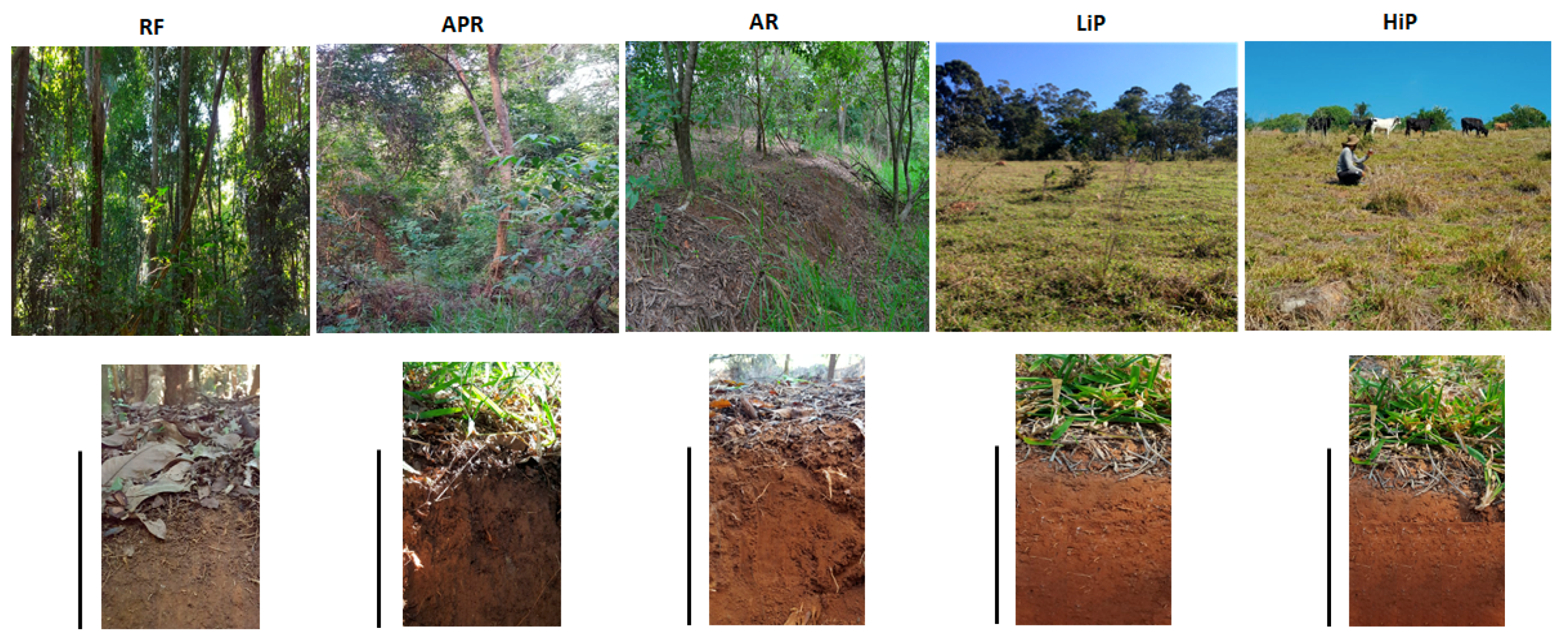
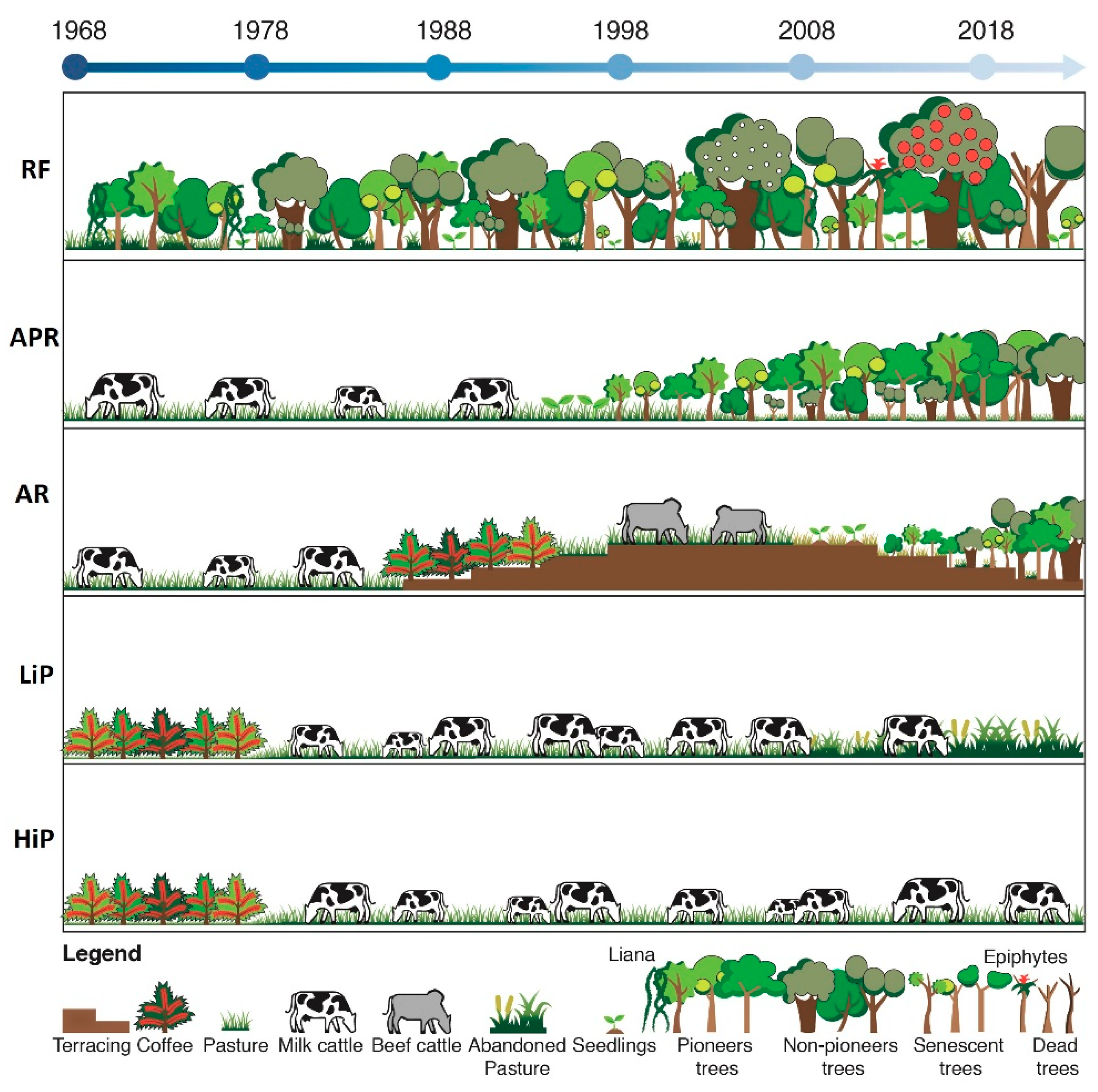
2.1. Study Area

The study area is located in the county of Campinas (22°53′ S, 46°54′ W), São Paulo State, Southeast Brazil (Figure 1). The climate in this region is classified as Cwa according to the Köppen classification mean annual precipitation is 1700 mm and mean annual temperature is 20 °C, with dry winters and wet summers [34]. Our study sites are located at the transition between the Atlantic Plateau and the Peripheral Depression geomorphological provinces [35]. The soils are classified as Ultisols [36] and the original vegetation in this area is a seasonal semi-deciduous forest, belonging to the Atlantic Forest biome. This region is highly fragmented, because of 200 years of historical landscape changes [37]. In particular, our study area is located inside the sub-basin of the Atibaia River where the main land uses are native vegetation and pastureland, occupying 33% and 30% of the sub-basin, respectively. The native vegetation includes Atlantic Forest remnants with different sizes and ages [38].
Within this area, we selected five land uses to measure soil physical and hydraulic properties, vegetation structure and diversity (Figure 2). In general, the deforestation of our study area already existed at the beginning of the 19th century, with the objective of introducing coffee (Coffea arabica) plantations. However, after the crisis in coffee cultivation during the early 20th century, the plantations were gradually replaced by pastures.
Land use history for the study sites was reconstructed based on interviews with the local population and aerial photographs taken in 1968, 1978, 1994, 2005 and 2017. The site RF is a secondary old-growth forest characterized by having the highest slope between the study sites, which was 28.8 ± 4.9% (SD). The slope was measured in the study plots with laser distance meter. Site RF was used as a control area to assess reference values for soil physical and hydraulic properties. According to interviews, in the early 20th century, this site was affected by natural fire disturbances and it was partially cleared at least once in the past for agricultural purposes. Moreover, aerial photographs showed that forest cover in most of the area was established and has increased since 1968. In this context, all RF plots were located in sites with forest cover in the last 40 years.
Site APR is located adjacent to the LiP. The slope (28.1 ± 2.8%) was similar to the RF. From 1968 to 1994, it was used for milk cattle grazing. Then, the area was abandoned and remained without a specific land use until 2007, leaving the forest to naturally regrow over 12 years. In 2007, to decide the best restoration strategy for the area, the “Diagnostic” protocol proposed by Rodrigues et al. [37] was implemented. This protocol allowed identifying the initial environmental situation and evaluating the potential of autogenic restoration of the area. Considering that this site evidenced favorable abiotic and biotic conditions (e.g., naturally regenerating native plants) for native plant establishment, the restoration diagnosis was of fair potential for autogenic restoration. Thus, forest restoration techniques included the encouragement of regenerating individual native trees and shrubs by manual and chemical control of invasive grasses. Moreover, enrichment plantings with native tree species were also implemented in patches without natural regeneration. In this regard, our measurements reflect the effect of 11 years of APR on a soil with a previous second-growth forest.
At AR site, the slope (22.8 ± 1.7%) was lower than the RF and APR. Initially, this site was used for dairy cattle grazing from 1968 to 1986. Later, it was replaced by coffee (C. arabica) plantations until 1994. It is important to emphasize that, at the beginning of the coffee plantation phase, widespread terracing was implemented. Then, in 1994, the coffee was replaced by pastures with Urochloa brizantha for beef cattle grazing. In 2007, the “Diagnostic” protocol mentioned previously was implemented. Given that AR site evidenced very few spontaneously regenerating seedlings and degraded environmental conditions that limited the passive restoration strategy, the restoration diagnosis in this area was of very low potential for autogenic restoration. Thus, AR was implemented through a restoration model that aimed to provide economical insurance and ensure successional processes to landowners [37]. Restoration plantings were implemented as mixed plantation with high-diversity-mix of seedlings (>50 native trees species). During the planting, these species were organized in fourth groups (e.g., initial, filling, middle and final species) according to the rate of growth and commercial value. Initial species (e.g., Acacia polyphilla, Croton floribundus and Schinus terebinthifolius) can be harvested for fuel production in 10–15 years, and are characteristically fast-growing, providing fast soil coverage and beneficial initial conditions for other species growth. Filling species (e.g., Croton urucurana, Gochnatia polymorpha and Trema micrantha) are also fast-growing species planted in the same line as the species. Middle species (e.g., Astronium graveolens, Gallesia integrifolia and Machaerium stipitatum) can be harvested during Years 20–25, and are more valuable wood species that will replace the initial and filling species. Final species (e.g., Aspidosperma polyneuron, Cariniana estrellensis and Cariniana legalis) are narrow canopy and slow-growing species that can be harvested during Years 40–45 for luxury and finished carpentry. The species planted are listed in Table S1. The total density of seedling was 1660 ind·ha−1, in a 3 m × 2 m spacing, using mechanized soil preparation. Before planting, invasive grasses were controlled through herbicide application. Fertilizers and irrigation were applied at the time of planting and during the first year [37,39]. As a result, our measurement in this restoration site represent the effect of 11 years of active restoration on highly degraded soil, with an intense land use history.
Site LiP with a slope of 22.7 ± 2.1% is located adjacent to the HiP, and both sites share a similar land use history until 2008. Since this year, in the LiP, grazing has been intermittent and with low productivity (e.g., stocking rate lower than two livestock units per hectare). During our field campaign, the vegetative cover in the LiP was dominated by the same grass specie (U. brizantha), with a mean height about 50 cm and isolated native trees, shrub species and nonnative grasses scattered in the area were also evident (Figure 2). Consequently, our results reflect the influence of 40 years of grazing, with a lower land use intensity in the last decade.
At site HiP, the slope was 23.3 ± 3.2%. This site was covered by a coffee (C. arabica) plantation until 1968. Afterwards, the coffee was replaced by pasture, planting U. brizantha as grass species. Since 1978, this area has been heavily grazed with dairy cattle, supporting a stocking rate greater than two livestock units per hectare, with regular application of fertilizers and other inputs. As a result, our measurements at this site represent the effect of 40 years of continuous grazing.
A graphical summary of the land use history for the five land uses described previously is provided in Figure 3.

2.2. Experimental Design

The study sites were located in a similar landscape position along the hillslope gradient and were selected to have the same soil type following Zwartendijk et al. [23]. In forest stands, we established four plots, and for the pasture sites three plots were established. Sampling the same number of plots per land uses was impossible due the restricted accessibility in pasture sites, resulting in 18 plots altogether (Figure 1). For sampling vegetation and soil attributes, the size of each plot was 500 m2 (50 m long and 10 m wide), a total area of 2000 m2 for each site. The size and number of plots were chosen according to similar investigations aimed at evaluating vegetation structure and composition in tropical forest restoration projects [40,41,42].

2.3. Vegetation Sampling

Vegetation sampling was conducted from September to November 2017 in the RF, APR and AR plots. In each 500 m2 plot, we identified and sampled all living trees and shrubs with height ≥ 50 cm and diameter at breast height (DBH) > 5 cm. Additionally, we installed a 200 m2 (50 m long and 4 m wide) subplot at the center of each plot, to identify and measure all trees and shrubs with DBH < 5 cm and height ≥ 50 cm. For all sites considered in this investigation, we measured the following vegetation attributes: (1) tree basal area; (2) canopy cover; (3) vegetation height; (4) tree density; and (5) species richness. These are key ecological indicators, useful to evaluate vegetation structure and composition in tropical forest restoration projects, also, they are being recommend in Atlantic Forest monitoring protocols [42,43]. As suggested by Viani et al. [42], the percentage of canopy cover in each plot was measured by an adaptation of the line interception method [44], installing a 50 m line transect in the middle of each study plot. Vegetation height was measured with a 5 m measuring stick, and the remaining height of trees taller than this was estimated visually. As suggested by Suganuma and Durigan [40], for tree density, we analyzed: (1) density of trees (DBH > 5 cm); and (2) density of saplings (DBH 1–5 cm). In the same way, for species richness, we analyzed: (1) total richness (all individual sampled); (2) overstory richness (DBH > 5 cm); and (3) richness of saplings (DBH 1–5 cm). For all previous ecological indicators, we calculated the mean values per study site. In addition, for all sampled individuals we classified the species origin as: native or nonnative to the study region. Specifically, in the AR site, we evaluated planted tree mortality.

2.4. Soil Sampling

Soil sampling was conducted during the dry season in April 2018. In the middle of each plot, we installed a 50 m transect along the hillslope gradient. At intervals of 15 m, three disturbed soil samples at 0–5 cm depth were collected. Before soil sampling, the litter and a small layer of soil (e.g., organic horizon) of less than 1 cm was removed. We determined the soil particle size distribution (PSD) with sand particle separation, the particle density (Pd) and soil organic carbon content (OC). The PSD analyses were carried out according to the hydrometer method [45]. Then, soil textures were classified following the USDA standards. The Pd was determined using the helium gas pycnometer method [46], and the OC analyses were performed following the Walkley–Black method [47]. In the same transects, at 7 m intervals, soil hydraulic measurements were conducted. In the specific case of AR site, to minimize spatial variability and possible induced effects by tillage, we placed the seven sampling points in the inter-plant space of planting lines. At each sampling point, we performed the Beerkan method [48,49]. A total of 126 Beerkan experiments were carried out, using a steel ring with an inner diameter of 16 cm inserted to a depth of about 1 cm into the soil surface. In each infiltration point, a known volume of water (150 mL) was repeatedly poured into the cylinder at a small height above soil surface (e.g., a few cm) and the energy of the water was dissipated with the hand fingers to minimize the soil disturbance. Then, the time needed for complete infiltration was logged. This procedure was repeated until the difference in infiltration time between two or three consecutives trials became negligible. Following a procedure commonly used for Beerkan method, at the beginning of each infiltration run, and near the steel ring, we collected one undisturbed soil core (100 cm3) at 0–5 cm depth to determine the bulk density (ρb) and the initial volumetric soil water content (θi). Saturated soil hydraulic conductivity (Ks) values were estimated by the Steady version of the Simplified method based on a Beerkan Infiltration run (SSBI method) [50]. According to previous a investigation carried out by Lozano-Baez et al. [28] on the same area, this method was chosen to avoid uncertainties due to a specific shape of the cumulative infiltration [51,52].
In addition, the undisturbed soil cores were used to determine total soil porosity (Pt), soil microporosity (Mic) and soil macroporosity (Mac). The Pt was calculated using ρb and mean Pd of each plot [53]. The Mic was estimated using a tension table with application of 6 kPa suction, and Mac was obtained by the difference between Pt and Mic [54]. Finally, according to Lassabatere et al. [48], at the end of each infiltration test, a disturbed soil sample was collected to determine the saturated gravimetric water content, and ρb was used to calculate the saturated volumetric soil water content (θs).

2.5. Data Analysis

The hypothesis of normal distribution of both the raw and the log-transformed data was tested by the Kolmogorov–Smirnov test. One-way analysis of variance (ANOVA) was performed with raw or log-transformed data. When ANOVA null hypothesis was rejected, we used multiple comparisons to detect differences between pairs by applying the Tukey’s honestly significant difference test. The related p-values were computed and compared to the level of significance of 0.05. Alternative non-parametric tests (Kruskal–Wallis ANOVA) were used when even the log-transformed data were non-normally distributed. In this case, when ANOVA null hypothesis was rejected, multiple comparisons between pairs were made with the Bonferroni method (adjusted p-values). Variables means were calculated for soil attributes according to the statistical distribution of the data, e.g., geometric mean for log-normal distributions and arithmetic means for normal distributions [55]. According to Lee et al., the appropriate CV expression for a log-normal distribution was calculated for the geometric means, and the usual CV was calculated for the arithmetic means [56]. Pearson’s correlation coefficient was calculated to identify correlation among the selected soil attributes: Pt, Mic, Mac, OC, θi, ρb and Ks across all study sites. Furthermore, to compare the soil and vegetation attributes among land use types, Principal Component Analysis (PCA) was performed on standardized variables. All statistical analyses were carried out using the Minitab© computer program (Minitab Inc., State College, PA, USA).

3. Results

3.1. Vegetation Attributes

A total of 541 saplings and 646 trees distributed in 38 families, 92 genera, and 138 species were sampled. For non-native species, we found 62 saplings and 147 trees, representing 11% and 23% of the total, respectively (Tables S2 and S3). Although the basal area and vegetation height of trees were much higher in RF, these did not differ statistically with both restored forests. The canopy cover showed significant differences in AR with RF and APR. We highlight the higher similarity between RF and APR for density of trees and saplings (Table 1), as a result of the high density of non-native trees Psidium guajava and Tecoma stans, which represented 24% and 5% of trees in APR, respectively. In contrast, non-native trees in the RF and AR represented 18% and 16%, respectively, of all tree individuals sampled in each site. Additionally, the total richness, the density and richness of trees and saplings were markedly lower in AR, where 14% of planted trees (e.g., initial species) were dead yet there was a higher presence of grasses (e.g., U. brizantha) observed in all plots.

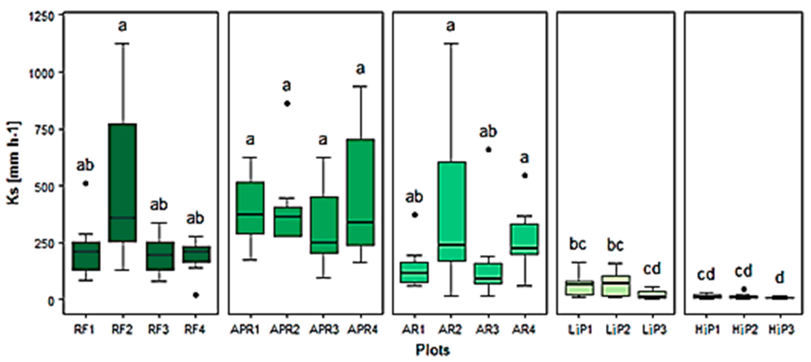
3.2. Soil Physical and Hydraulic Properties

The texture of the upper layers of the soil (0–5 cm) was clay loam in APR and pasture sites, while it was sandy clay loam in RF and AR sites. The clay content at the study sites ranged between 21% and 44%, but only the RF with lower values of clay differed significantly from the other study sites. Moreover, soil samples taken from the HiP showed the highest clay content. The silt ranged between 18% and 37%, with higher silt values in APR that differed significantly from other land-covers. The sand content varied between 31% and 55%, and was significantly lower in APR compared with other study sites (Table 2).
Comparisons of ρb values between study sites revealed higher similarity between RF and APR, while AR presented similar ρb values with both pasture sites. The Pd had similar values in all study sites, ranging from 2.61 to 2.71 g cm−3. The OC varied significantly among sites (from 4.6 to 25.6 g kg−1), with higher values in HiP and markedly lower values in AR. The soil Mac ranged from 0.16 to 0.38 cm3 cm−3, with greater values observed in RF, followed by the APR, AR, LiP and HiP. Similar results were obtained for Pt, which varied from 0.48 to 0.66 cm3 cm−3. In contrast, the soil Mic (from 0.21 to 0.43 cm3 cm−3) was much higher in pasture sites and decreased in forest land-covers, with lower values in RF and AR. In addition, the θi at the time of the Beerkan infiltration run varied between 0.12 and 0.32 cm3 cm−3, with significant lower values in the RF. The θs varied between 0.29 and 0.75 cm3 cm−3 with significant lower values in restored forests. The Ks at the soil surface in the study land uses ranged from 4 mm h−1 to a maximum of 1121 mm h−1. The higher Ks was evidenced in APR, which was only similar with RF and significantly different from other three land uses. The Ks values obtained in the RF were lower than APR. In contrast, the Ks of AR between 15 and 1121 mm h−1 was similar to RF and differed significantly for the other three land uses. In addition, across the five land uses, Ks values varied least and differed significantly from each other at the LiP and HiP (Table 3).
Within-site plots, high variability in Ks was observed in the RF plots and within the two restored forest classes. In contrast, smaller variations were evidenced in pasture sites. Figure 4 includes the results of the of the Tukey’s test for all sampled plots. The grouping information highlights the significant and non-significant comparisons for all sampled plots. In the first group, the forest plots evidenced not significant differences due to the high Ks variability within these plots (e.g., Ks means from 104 to 407 mm h–1). Then, the second group (RF1, RF3, RF4, AR1, AR3, LiP1 and LiP2) showed significant differences with pasture sites, which were grouped in a third (LiP1, LiP2, LiP3, HiP1 and HiP2) and fourth group (LiP3, HiP1, HiP2 and HiP3). In general, the LiP and HiP plots were similar, and mean Ks values altogether (e.g., from 8 to 47 mm h–1) were very low (Figure 4).
According to the Pearson’s correlation coefficient among selected soil attributes across all study sites, significant positive correlations were found for Pt vs. Mac (0.60) and Ks vs. Mac (0.67). In contrast, significant negative correlations were found for ρb vs. Pt (−0.99), ρb vs. Mac (−0.58) and Ks vs. Mic (−0.49) (Figure S1).
The first and second axis of the PCA for the soil attributes explained 43.0% and 29.3%, respectively, of the variation among all study sites. This analysis revealed a gradient of land-cover types from pastures to forest covers. As expected, the pasture sites were separated from the forest covers due to the higher Mic and ρb. Similarly, the higher ρb values in AR plots contributed to separating the study site. Then, APR plots were more similar to RF plots, and both forest covers were associated with higher Ks, Mac, Pt, θi and OC values (Figure 5A). The PCA correlating the soil and vegetation attributes showed a clear segregation among forest cover sites, explaining 55.2% and 16.5% of the variation in the first and second axis, respectively. This analysis showed that RF plots were mainly related with larger trees, evidencing higher correlation with vegetation attributes such as height of trees, density of saplings, basal area, canopy cover and overstory richness, also it was evidenced intermediate values of Mic. Considering the vegetation attributes in APR plots, the PCA showed positive correlation with total richness of species, density of trees and richness of saplings, also positive correlation and higher values of Ks, θi, Mac and Pt were found in these plots. By contrast, the separation of AR plots was driven by the higher ρb values and lower vegetation attributes, since AR site had a more intensive land use history compared to RF and APR sites. In particular, among AR plots, AR3 was the most different plot, composed by few and smaller trees growing in a compacted soil (Figure 5B).

4. Discussion

4.1. Effects of Land-Cover Type and Land Use History on Soil Physical and Hydraulic Properties

Assessing the Ks recovery, soil physical and hydraulic properties of different forest restoration strategies, and investigating their relationships with land use history, vegetation structure and composition, provided the opportunity to identify the extent to which these forest restoration strategies contribute to supplying ecosystem functions as infiltration of rainwater. The variation of Ks among land-cover types was not as we expected, due to the higher Ks evidenced in APR and lower in RF. However, our results supported the first study hypothesis, namely that a more intensive land use history in AR resulted in a lower Ks recovery compared to APR. Importantly, despite both restored forest types being located in the same soil type and landscape position, it was not clear from our measurements whether APR resulted in a faster recovery of Ks compared to AR, due to the high variability in land use history. Similar situations have been reported in several tropical studies [26,29]. In addition, the Ks recovery in APR could be associated with improved soil physical and hydraulic properties, which suggest a higher soil pore connectivity. Hassler et al. [12] found similar Ks at 0–6 cm depth between 100-year-old and 12–15-year-old secondary forests in Panama. Similarly, Leite et al. [24], at Brazilian Caatinga, obtained no significant differences for surface Ks between old-growth forest (more than 55 years) and young secondary forest (7 years). This Ks recovery to pre-pasture levels was also detected at 12.5 cm depth after 15 years of pasture abandonment for an Oxisol in the Brazilian Amazon [11] and by other studies carried out in tropical environments [20,21]. In contrast, after 10 years of natural regeneration in Ecuador, no significant changes of Ks were reported at 12.5 cm depth for an Inceptisol, which was related with invasive species delaying the Ks recovery [33].
Our Ks in the RF plots can be compared with those for Lozano-Baez et al. [28], as both investigations in the same forest biome estimated the Ks with the SSBI method, on the same soil texture (e.g., sandy clay loam) and at the same soil depth used an identical measurement technique (e.g., Beerkan method) and instruments. Our mean Ks in the RF (215 mm h−1) was close to reported value (387 mm h−1) by Lozano-Baez et al. [28] under similar soil conditions. This difference can be explained by the more conserved soil conditions in the study area of Lozano-Baez et al. [28], for example, as their remnant forest was never burned or cultivated. In contrast, our RF was partially cleared and was affected by natural fire disturbances. This observation is in line with several studies, which suggest that in old-growth tropical forests the Ks can be affected by past soil degradation and intensity of forest use [11,15,29,57]. The Ks values obtained in RF plots (e.g., from 23 to 1122 mm h−1) showed the high spatial variability of the infiltration process under forest cover, which can be associated with the heterogeneous soil structure, lower ρb and higher Mac [57,58,59]. Another factor to consider is the spatial heterogeneity of our RF, where different landscape conditions such as higher slope and vegetation attributes among sample plots could have influenced the Ks variability. In this sense, we believe that the true reference soil condition could be represented by RF plot RF2, due to observed low soil disturbance in this plot, which is consistent with the higher tree basal area (39.4 m2 ha−1), vegetation height (average of 12.9 m), species richness (41 trees and non-tree; Table 1 and Table S4), OC and soil porosity (Table 3 and Table S5). Unfortunately, it was not possible to find similar forests in the study area, but we could expect that infiltration capacity in other Brazilian Atlantic Forest patches will be directly related with the forest age and forest conditions, which has been shown by several studies [12,24,60]. Therefore, the Ks values in RF could be limited by the number of measurements (n = 28), which should be increased in future studies, considering the gradient and spatial heterogeneity of forest cover.
Our results highlight the importance of land use legacy on Ks recovery after forest restoration. The restoration diagnosis in APR and AR based on the “Diagnostic” protocol [37], allowed evidencing significant differences in the initial environmental situations (e.g., naturally regenerating native plants) and land use history between both sites. In fact, the initial differences in the initial environmental situations in each restored site allowed the restoration practitioners to identify and select at the beginning of the restoration project the most suitable restoration strategy. Figure 3 provides a graphical summary of these differences between APR and AR. Our findings are also in agreement with other studies that reported lower Ks when land use was more intense prior to forest regrowth [11,21,27]. In this sense, our AR site with a more intensive land use history, resulted in significant lower Ks, which could be attributed mainly to greater soil exposure and soil compaction during the land use history. Our mean Ks in the AR site (163 mm h−1) was considerably higher than the reported value (54 mm h−1) by Lozano-Baez et al. [28] on the same soil texture (e.g., sandy clay loam). This difference can be explained by the higher ρb values found in the actively restored forest of Lozano-Baez et al. [28].
Despite no statistically significant differences being found between AR and other forest plots, we stress that the specific past land use intensity and management in each plot could also have played an important role in soil degradation. Thus, we found AR plots (AR1 and AR3), where the Ks values were below the mean of other forest plots. The lower Ks in these plots are consistent with their higher ρb and Mic, lower Mac and OC (Table S5) and possibly a more intensive past management, suggesting that these plots still retain the “memory” from the previous land use. Similar results have been reported by Bonell et al. [26], for a 10-year-old Acacia plantation in India growing in Ultisols and Oxisols, with lower Ks when compared to less disturbed forests. On the other hand, the higher Ks in restored plots AR2 and AR4 is closer to the RF and APR plots, indicating that in some cases after 11 years the active restoration could reach the infiltration recovery target defined by the reference conditions. This finding agrees with recent literature reviews, which show that Ks recovery after tree planting in the tropics occur across a wide range of soil conditions [61,62] and probably after more than one decade [26,33]. In addition, it is important to underscore that before tree planting at AR site, trampling pressure occurred for 13 years over abandoned agricultural terraces, causing terracing failure. Several previous studies have reported an increase in soil loss, surface runoff, ρb and reduction of infiltration rates after terrace abandoning [63,64]. Another important factor that might have influenced the current Ks in AR site is the possible soil compaction during soil preparation, tree planting using bulldozers or tractors is associated with high levels of soil disturbance, and the effects of this soil preparation can persist long after tree planting [65]. Overall, these circumstances suggest that initial soil conditions before forest restoration actions at AR site were more degraded than in APR. Nevertheless, in our study the lack of soil measurements in each moment of the land use history precludes a stronger understanding of the relative impacts of historical land management on Ks recovery, thus future studies should consider the role of previous land use, comparing sites with a truly identical history.
The significantly lower Ks observed in pasture sites compared to forest land-cover types was consistent with several previous studies [20,33,66], supporting the importance of preserving the forest cover and promoting forest restoration actions in the landscape to maintain the infiltration process. This result can be attributed to higher ρb and Mic in both pasture sites (Table 3). In the present study, we observed a significant higher Ks in the LiP compared to HiP. The differences in Ks between LiP and HiP are mainly related to factors such as cattle-grazing intensity and the duration of pasture cover, which has been similarly reported in several other tropical studies [11,12,66]. Additionally, the similar OC between pasture sites and forest covers (RF and APR) is a trend that has been previously noted by other authors [9,22,28,67], suggesting that such similarities are linked to the accumulation of organic matter by the root system of grasses, the animal-derived inputs and application of fertilizers.

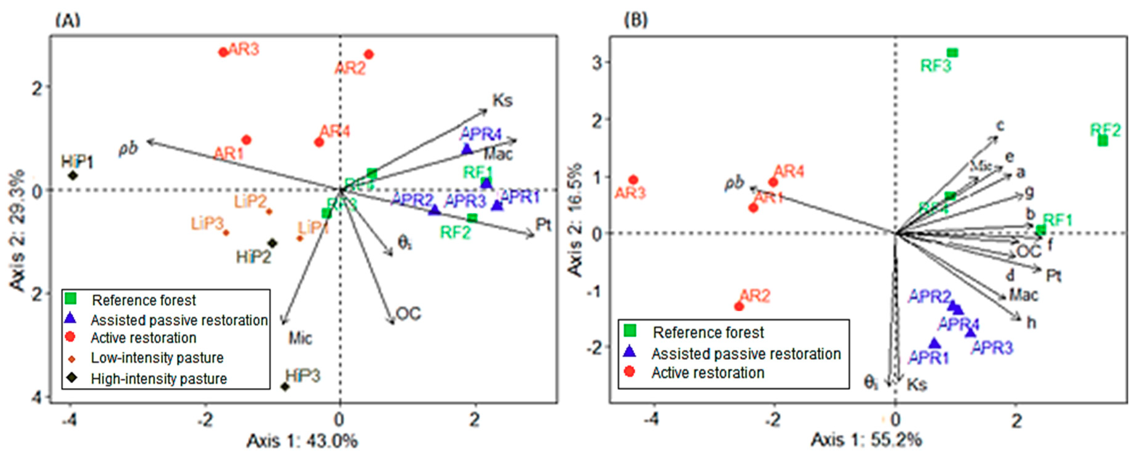
4.2. Relationships between Soil, Vegetation and Land Use History

When evaluating vegetation attributes in forest cover sites, our study revealed the significantly lower values in AR and higher values in RF. The higher values of vegetation attributes in the RF could be explained as a consequence of the longer time that this old-growth forest (Figure 3) has remained undisturbed [68,69]. It is interesting to note that basal area and vegetation height of trees in AR could reach statistically similar values to the RF. Similarly, Garcia et al. [70] found in the same biome no significant differences in the basal area between actively restored forests (12, 23 and 55 years old) and the reference condition. Furthermore, it is noteworthy in AR that, while Ks, basal area and vegetation height of trees have reached statistically similar values with the RF, other vegetation attributes, such as canopy cover, tree density and species richness, were significantly lower than those for the RF plots. For instance, the lower canopy cover, density and richness of saplings (e.g., lack of regenerating trees) in AR might compromise the future forest structure [68], which could hamper the recovery of soil hydraulic properties [62]. Although the herbaceous cover was not directly quantified, we observed a higher abundance of grasses (e.g., U. brizantha) in AR site, which could be related to the lower canopy cover. The open canopy conditions in AR may have favored the persistence of grasses, hindering the recruitment of new trees species [71]. In contrast, APR site had statistically similar Ks (Figure 4) and vegetation attributes to the RF (Table 1). However, the vegetation attributes in APR were mainly influenced by non-native trees, such as P. guajava, an aggressive pioneer species with allelopathic potential [72]. For these reasons, we suggest that both restored forests need management activities to improve soil and vegetation attributes. Canopy cover protects the soil from physical disturbance, and higher species richness and tree density with native species can produce a higher biomass and enhance the Ks [73,74].
One possible explanation for the different outputs between AR and APR are the initial soil conditions at each site. As mentioned above, when the forest restoration actions began in APR, the soil might have had better initial conditions (lower ρb, higher Ks, OC and soil porosity), and some degree of natural regeneration, which stimulated the potential recovery of the site and facilitating the recruitment of new trees species [3,37]. In AR site, the more intensive land use history probably led to an area with low resilience, a more compacted soil and poor OC. In particular, the intensity of past land use has been reported as the main factor affecting tropical forest recovery, for example, the vegetation in pastures with a long-lasting land use will regenerate more slowly relative to pastures used less intensively [75,76]. Both restoration approaches (APR and AR) have an important role in the process of restoring degraded ecosystems in tropical landscapes and can be used complementary to enhance the chances of restoration success [37,68]. To understand the soil hydraulic recovery after forest restoration, it is important that future studies consider the role of the duration and intensity of the previous land use, including parameters to assess the land use legacy effects [11,77] and more measurements over time in deeper soil layers, which may reveal further differences among restoration strategies.
The correlation results for Pt vs. Mac and Ks vs. Mac are in agreement with several other studies in the Atlantic Forest [30,58], which reported the positive influence of Mac for the pore space and infiltration process. This finding is consistent with the inverse relationships between Ks vs. ρb, Ks vs. Mic and Mac vs. ρb, also found by some studies [9,23,28,78]. High OC contributes to the trend of increasing Ks, soil porosity and reducing ρb values [9]. However, the reverse occurred in the present study, which can be attributed to the high OC and ρb in pastures sites as well as low OC in AR but with a high Ks, suggesting that recovery of soil physical and hydraulic properties is not only dependent on the OC. The result of the PCA indicate the importance of forest cover to promote the infiltration and better soil physical and hydraulic properties. This could be associated with the litter inputs, roots and higher soil faunal activity produced by the trees, which can influence positively the aggregate stability, Mac and OC, thereby Ks increase in forest covers [79,80]. Nevertheless, there is a need to further research the plant–soil interactions; for example, little attention has been paid to the effects of individual trees, richness and density of species on Ks and soil hydraulic properties [80].

5. Conclusions

The Ks recovery differed between AR and APR sites. As we expected, the knowledge of the land use history was crucial for understanding the current differences among the study sites for Ks, soil physical and hydraulic properties. This is consistent with our previous work [28] in the same forest restoration program. The Ks and vegetation attributes decreased when land use was more intense prior to forest restoration actions. The influence of land use intensity on soil physical and hydraulic properties could also be evidenced in the comparison between LiP and HiP. The present results further illustrate the positive correlation between Ks and vegetation attributes (tree basal area, vegetation height of trees and overstory richness) in forests undergoing restoration.

Supplementary Materials

The following are available online at https://www.mdpi.com/2073-4441/11/1/86/s1, Figure S1: Correlogram showing the Pearson correlations coefficients between soil attributes across the study sites: Reference Forest, Assisted Passive Restoration, Active Restoration, Low-intensity Pasture and High-intensity Pasture. Table S1: List of species used in the Active Restoration site. Table S2: Species list of the trees with DBH > 5 cm sampled in the studies sites: Reference Forest, Assisted Passive Restoration and Active Restoration. Table S3: Species list of the trees with DBH 1–5 cm sampled in the studies sites: Reference Forest, Assisted Passive Restoration and Active Restoration. Table S4: Vegetation attributes across the study plots. Table S5: Mean for soil attributes in the depth 0–5 cm across the study plots.

Author Contributions

S.E.L.-B. carried out the data collection and wrote the initial draft. M.C. participated in the design of the study and helped to draft and edit the manuscript. S.F.d.B.F. and R.R.R. provided important advice on the concept of structuring of the manuscript and supervised the study. M.C. and S.D.P. analyzed the data and made great contributions to writing the manuscript. All authors reviewed and approved the final manuscript.

Funding

This research was supported by the Fundação de Amparo à Pesquisa do Estado de São Paulo (BIOTA/FAPESP Program: 2013/50718-5 and 1999/09635-0), and Conselho Nacional de Desenvolvimento Científico e Tecnológico (CNPq 561897/2010-7 and Miguel Cooper’s, Ricardo Ribeiro Rodrigues’s and Silvio Frosini de Barros Ferraz’s scientific productivity fellowships).

Acknowledgments

We would like to thank Carolina Bozetti Rodrigues and Luiz Felippe Salemi for their valuable suggestions. We are grateful for Vanessa Erler Sontag who illustrated the land use history, as well as for the taxonomist and researchers who assisted the plant species identification: Vinicius Castro Souza, Fabiano Turini Farah, Thiago Bevilacqua, Gabriel Dalla Colleta and Marcelo Antonio Pinho Ferreira. We thank Daigard Ricardo Ortega, Monica Borda, Miller Ruiz, Raissa Corrêa de Andrade, Renato de Oliveira, Nayana Alves Pereira, Glaucia Santos, Aline Franzosi and all field assistants for their company and help in the field. The authors also would like to thank the landowners who allowed the forest sampling and anonymous reviewers for their constructive comments.

Conflicts of Interest

The authors declare no conflict of interest.

References

  1. Chazdon, R.L. Beyond deforestation: Restoring forests and ecosystem services on degraded lands. Science 2008, 320, 1458–1460. [Google Scholar] [CrossRef]
  2. Keenan, R.J.; Reams, G.A.; Achard, F.; de Freitas, J.V.; Grainger, A.; Lindquist, E. Dynamics of global forest area: Results from the FAO Global Forest Resources Assessment 2015. For. Ecol. Manag. 2015, 352, 9–20. [Google Scholar] [CrossRef] [Green Version]
  3. Rodrigues, R.R.; Gandolfi, S.; Nave, A.G.; Aronson, J.; Barreto, T.E.; Vidal, C.Y.; Brancalion, P.H.S. Large-scale ecological restoration of high-diversity tropical forests in SE Brazil. For. Ecol. Manag. 2011, 261, 1605–1613. [Google Scholar] [CrossRef]
  4. Shono, K.; Cadaweng, E.A.; Durst, P.B. Application of assisted natural regeneration to restore degraded tropical forestlands. Restor. Ecol. 2007, 15, 620–626. [Google Scholar] [CrossRef]
  5. Zahawi, R.A.; Reid, J.L.; Holl, K.D. Hidden costs of passive restoration: Passive restoration. Restor. Ecol. 2014, 22, 284–287. [Google Scholar] [CrossRef]
  6. Holl, K.D.; Aide, T.M. When and where to actively restore ecosystems? For. Ecol. Manag. 2011, 261, 1558–1563. [Google Scholar] [CrossRef]
  7. Badalamenti, E.; da Silveira Bueno, R.; Campo, O.; Gallo, M.; La Mela Veca, D.; Pasta, S.; Sala, G.; La Mantia, T. Pine stand density influences the regeneration of Acacia saligna Labill. H.L. Wendl. and native woody species in a mediterranean coastal pine plantation. Forests 2018, 9, 359. [Google Scholar] [CrossRef]
  8. Crouzeilles, R.; Ferreira, M.S.; Chazdon, R.L.; Lindenmayer, D.B.; Sansevero, J.B.B.; Monteiro, L.; Iribarrem, A.; Latawiec, A.E.; Strassburg, B.B.N. Ecological restoration success is higher for natural regeneration than for active restoration in tropical forests. Sci. Adv. 2017, 3, 1–7. [Google Scholar] [CrossRef]
  9. Gageler, R.; Bonner, M.; Kirchhof, G.; Amos, M.; Robinson, N.; Schmidt, S.; Shoo, L.P. Early response of soil properties and function to riparian rainforest restoration. PLoS ONE 2014, 9, e104198. [Google Scholar] [CrossRef]
  10. Mendes, M.S.; Latawiec, A.E.; Sansevero, J.B.B.; Crouzeilles, R.; de Moraes, L.F.D.; Castro, A.; Pinto, H.N.A.; Brancalion, P.H.S.; Rodrigues, R.R.; Chazdon, R.L.; et al. Look down—There is a gap—The need to include soil data in Atlantic Forest restoration: Scarcity of soil data in restoration. Restor. Ecol. 2018. [Google Scholar] [CrossRef]
  11. Zimmermann, B.; Elsenbeer, H.; De Moraes, J.M. The influence of land-use changes on soil hydraulic properties: Implications for runoff generation. For. Ecol. Manag. 2006, 222, 29–38. [Google Scholar] [CrossRef]
  12. Hassler, S.K.; Zimmermann, B.; van Breugel, M.; Hall, J.S.; Elsenbeer, H. Recovery of saturated hydraulic conductivity under secondary succession on former pasture in the humid tropics. For. Ecol. Manag. 2011, 261, 1634–1642. [Google Scholar] [CrossRef]
  13. Zimmermann, A.; Schinn, D.S.; Francke, T.; Elsenbeer, H.; Zimmermann, B. Uncovering patterns of near-surface saturated hydraulic conductivity in an overland flow-controlled landscape. Geoderma 2013, 195–196, 1–11. [Google Scholar] [CrossRef]
  14. Alagna, V.; Di Prima, S.; Rodrigo-Comino, J.; Iovino, M.; Pirastru, M.; Keesstra, S.; Novara, A.; Cerdà, A. The impact of the age of vines on soil hydraulic conductivity in vineyards in eastern Spain. Water 2017, 10, 14. [Google Scholar] [CrossRef]
  15. Di Prima, S.; Marrosu, R.; Lassabatere, L.; Angulo-Jaramillo, R.; Pirastru, M. In situ characterization of preferential flow by combining plot- and point-scale infiltration experiments on a hillslope. J. Hydrol. 2018, 563, 633–642. [Google Scholar] [CrossRef]
  16. Cullotta, S.; Bagarello, V.; Baiamonte, G.; Gugliuzza, G.; Iovino, M.; La Mela Veca, D.S.; Maetzke, F.; Palmeri, V.; Sferlazza, S. Comparing different methods to determine soil physical quality in a mediterranean forest and pasture land. Soil Sci. Soc. Am. J. 2016, 80, 1038–1056. [Google Scholar] [CrossRef]
  17. Di Prima, S.; Bagarello, V.; Angulo-Jaramillo, R.; Bautista, I.; Cerdà, A.; del Campo, A.; González-Sanchis, M.; Iovino, M.; Lassabatere, L.; Maetzke, F. Impacts of thinning of a Mediterranean oak forest on soil properties influencing water infiltration. J. Hydrol. Hydromech. 2017, 65, 276–286. [Google Scholar] [CrossRef] [Green Version]
  18. Elrick, D.E.; Reynolds, W.D. Methods for analyzing constant-head well permeameter data. Soil Sci. Soc. Am. J. 1992, 56, 320–323. [Google Scholar] [CrossRef]
  19. Deb, S.K.; Shukla, M.K. Variability of hydraulic conductivity due to multiple factors. Am. J. Environ. Sci. 2012, 8, 489–502. [Google Scholar] [CrossRef]
  20. Godsey, S.; Elsenbeer, H. The soil hydrologic response to forest regrowth: A case study from southwestern Amazonia. Hydrol. Process. 2002, 16, 1519–1522. [Google Scholar] [CrossRef]
  21. Ziegler, A.D.; Giambelluca, T.W.; Tran, L.T.; Vana, T.T.; Nullet, M.A.; Fox, J.; Vien, T.D.; Pinthong, J.; Maxwell, J.; Evett, S. Hydrological consequences of landscape fragmentation in mountainous northern Vietnam: Evidence of accelerated overland flow generation. J. Hydrol. 2004, 287, 124–146. [Google Scholar] [CrossRef]
  22. Paul, M.; Catterall, C.P.; Pollard, P.C.; Kanowski, J. Recovery of soil properties and functions in different rainforest restoration pathways. For. Ecol. Manag. 2010, 259, 2083–2092. [Google Scholar] [CrossRef]
  23. Nyberg, G.; Bargués Tobella, A.; Kinyangi, J.; Ilstedt, U. Soil property changes over a 120-yr chronosequence from forest to agriculture in western Kenya. Hydrol. Earth Syst. Sci. 2012, 16, 2085–2094. [Google Scholar] [CrossRef] [Green Version]
  24. Leite, P.A.M.; de Souza, E.S.; dos Santos, E.S.; Gomes, R.J.; Cantalice, J.R.; Wilcox, B.P. The influence of forest regrowth on soil hydraulic properties and erosion in a semiarid region of Brazil. Ecohydrology 2017, 11, 1–12. [Google Scholar] [CrossRef]
  25. Mapa, R.B. Effect of reforestation using Tectona grandis on infiltration and soil water retention. For. Ecol. Manag. 1995, 77, 119–125. [Google Scholar] [CrossRef]
  26. Bonell, M.; Purandara, B.K.; Venkatesh, B.; Krishnaswamy, J.; Acharya, H.A.K.; Singh, U.V.; Jayakumar, R.; Chappell, N. The impact of forest use and reforestation on soil hydraulic conductivity in the Western Ghats of India: Implications for surface and sub-surface hydrology. J. Hydrol. 2010, 391, 47–62. [Google Scholar] [CrossRef]
  27. Ghimire, C.P.; Bruijnzeel, L.A.; Bonell, M.; Coles, N.; Lubczynski, M.W.; Gilmour, D.A. The effects of sustained forest use on hillslope soil hydraulic conductivity in the Middle Mountains of Central Nepal: Sustained forest use and soil hydraulic conductivity. Ecohydrology 2014, 7, 478–495. [Google Scholar] [CrossRef]
  28. Lozano-Baez, S.; Cooper, M.; Ferraz, S.; Ribeiro Rodrigues, R.; Pirastru, M.; Di Prima, S. Previous land use affects the recovery of soil hydraulic properties after forest restoration. Water 2018, 10, 453. [Google Scholar] [CrossRef]
  29. Zwartendijk, B.W.; van Meerveld, H.J.; Ghimire, C.P.; Bruijnzeel, L.A.; Ravelona, M.; Jones, J.P.G. Rebuilding soil hydrological functioning after swidden agriculture in eastern Madagascar. Agric. Ecosyst. Environ. 2017, 239, 101–111. [Google Scholar] [CrossRef]
  30. Cooper, M.; Rosa, J.D.; Medeiros, J.C.; de Oliveira, T.C.; Toma, R.S.; Juhász, C.E.P. Hydro-physical characterization of soils under tropical semi-deciduous forest. Sci. Agricol. 2012, 69, 152–159. [Google Scholar] [CrossRef] [Green Version]
  31. Ziter, C.; Graves, R.A.; Turner, M.G. How do land-use legacies affect ecosystem services in United States cultural landscapes? Landsc. Ecol. 2017, 32, 2205–2218. [Google Scholar] [CrossRef]
  32. Foster, D.; Swanson, F.; Aber, J.; Burke, I.; Brokaw, N.; Tilman, D.; Knapp, A. The importance of land-use legacies to ecology and conservation. BioScience 2003, 53, 77–88. [Google Scholar] [CrossRef]
  33. Zimmermann, B.; Elsenbeer, H. Spatial and temporal variability of soil saturated hydraulic conductivity in gradients of disturbance. J. Hydrol. 2008, 361, 78–95. [Google Scholar] [CrossRef] [Green Version]
  34. Mello, M.H.; Pedro Junior, M.J.; Ortolani, A.A.; Alfonsi, R.R. Chuva e Temperatura: Cem Anos de Observações em Campinas; Boletim Tecnico; IAC: Campinas, Brazil, 1994. [Google Scholar]
  35. de Oliveira, L.H.d.S.; Valladares, G.S.; Coelho, R.M.; Criscuolo, C. Soil vulnerability to degradation at Campinas municipality, SP. Geografia (Londrina) 2014, 22, 65–79. [Google Scholar]
  36. Soil Survey Staff. Keys to Soil Taxonomy, 12th ed.; USDA-Natural Resources Conservation Service: Washington, DC, USA, 2014.
  37. Rodrigues, R.R.; Lima, R.A.F.; Gandolfi, S.; Nave, A.G. On the restoration of high diversity forests: 30 years of experience in the Brazilian Atlantic Forest. Biol. Conserv. 2009, 142, 1242–1251. [Google Scholar] [CrossRef]
  38. Molin, P.G.; Gergel, S.E.; Soares-Filho, B.S.; Ferraz, S.F.B. Spatial determinants of Atlantic Forest loss and recovery in Brazil. Landsc. Ecol. 2017, 32, 857–870. [Google Scholar] [CrossRef]
  39. Preiskorn, G.M.; Pimenta, D.; Amazonas, N.T.; Nave, A.G.; Gandolfi, S.; Rodrigues, R.R.; Belloto, A.; Cunha, M.C.S. Metodologia de restauração para fins de aproveitamento econômico (reservas legais e áreas agrícolas). In Pacto Pela Restauração da Mata Atlântica—Referencial dos Conceitos e ações de Restauração Florestal; Rodrigues, R.R., Brancalion, P.H.S., Eds.; LERF/ESALQ: Instituto BioAtlântica: São Paulo, Brazil, 2009; pp. 158–175. ISBN 978-85-60840-02-1. [Google Scholar]
  40. Suganuma, M.S.; Durigan, G. Indicators of restoration success in riparian tropical forests using multiple reference ecosystems: Indicators of riparian forests restoration success. Restor. Ecol. 2015, 23, 238–251. [Google Scholar] [CrossRef]
  41. Toledo, R.M.; Santos, R.F.; Baeten, L.; Perring, M.P.; Verheyen, K. Soil properties and neighbouring forest cover affect above-ground biomass and functional composition during tropical forest restoration. Appl. Veg. Sci. 2018, 21, 179–189. [Google Scholar] [CrossRef]
  42. Viani, R.A.G.; Barreto, T.E.; Farah, F.T.; Rodrigues, R.R.; Brancalion, P.H.S. Monitoring young tropical forest restoration sites: How much to measure? Trop. Conserv. Sci. 2018, 11, 1–9. [Google Scholar] [CrossRef]
  43. Chaves, R.B.; Durigan, G.; Brancalion, P.H.S.; Aronson, J. On the need of legal frameworks for assessing restoration projects success: New perspectives from São Paulo state (Brazil): Legal instruments for assessing restoration. Restor. Ecol. 2015, 23, 754–759. [Google Scholar] [CrossRef]
  44. Canfield, R. Application of line interception method in sampling range vegetation. J. For. 1941, 39, 388–394. [Google Scholar] [CrossRef]
  45. Gee, G.; Or, D. Particle-size analysis. In Methods of Soil Analysis: Physical Methods; Dane, J.H., Topp, C., Eds.; Soil Science Society of America: Madison, WI, USA, 2002; pp. 255–293. ISBN 978-0-89118-841-4. [Google Scholar]
  46. Flint, A.L.; Flint, L.E. Particle density. In Methods of Soil Analysis: Physical Methods; Dane, J., Topp, G.C., Eds.; Soil Science Society of America: Madison, WI, USA, 2002; pp. 229–240. [Google Scholar]
  47. Walkley, A.; Black, I.A. An examination of the degtjareff method for determining soil organic matter, and a proposed modification of the chromic acid titration method. Soil Sci. 1934, 37, 29–38. [Google Scholar] [CrossRef]
  48. Lassabatère, L.; Angulo-Jaramillo, R.; Soria Ugalde, J.M.; Cuenca, R.; Braud, I.; Haverkamp, R. Beerkan estimation of soil transfer parameters through infiltration experiments—BEST. Soil Sci. Soc. Am. J. 2006, 70, 521. [Google Scholar] [CrossRef]
  49. Braud, I.; De Condappa, D.; Soria, J.M.; Haverkamp, R.; Angulo-Jaramillo, R.; Galle, S.; Vauclin, M. Use of scaled forms of the infiltration equation for the estimation of unsaturated soil hydraulic properties (the Beerkan method). Eur. J. Soil Sci. 2005, 56, 361–374. [Google Scholar] [CrossRef]
  50. Bagarello, V.; Di Prima, S.; Iovino, M. Estimating saturated soil hydraulic conductivity by the near steady-state phase of a Beerkan infiltration test. Geoderma 2017, 303, 70–77. [Google Scholar] [CrossRef]
  51. Alagna, V.; Iovino, M.; Bagarello, V.; Mataix-Solera, J.; Lichner, L. Alternative analysis of transient infiltration experiment to estimate soil water repellency. Hydrol. Process. 2018. [Google Scholar] [CrossRef]
  52. Di Prima, S.; Concialdi, P.; Lassabatere, L.; Angulo-Jaramillo, R.; Pirastru, M.; Cerdà, A.; Keesstra, S. Laboratory testing of Beerkan infiltration experiments for assessing the role of soil sealing on water infiltration. Catena 2018, 167, 373–384. [Google Scholar] [CrossRef]
  53. Danielson, R.E.; Sutherland, P.L. Porosity. In Methods of Soil Analysis. Part I. Physical and Mineralogical Methods. Agronomy Monograph No. 9; Klute, A., Ed.; American Society of Agronomy, Soil Science Society of America: Madison, WI, USA, 1986; pp. 443–461. [Google Scholar]
  54. EMBRAPA. Manual of Methods of Soil Analysis, 2nd ed.; Embrapa Soils: Rio de Janeiro, Brazil, 2011. [Google Scholar]
  55. Reynolds, W.D.; Drury, C.F.; Yang, X.M.; Tan, C.S. Optimal soil physical quality inferred through structural regression and parameter interactions. Geoderma 2008, 146, 466–474. [Google Scholar] [CrossRef]
  56. Lee, D.M.; Elrick, D.E.; Reynolds, W.D.; Clothier, B.E. A comparison of three field methods for measuring saturated hydraulic conductivity. Can. J. Soil Sci. 1985, 65, 563–573. [Google Scholar] [CrossRef]
  57. Scheffler, R.; Neill, C.; Krusche, A.V.; Elsenbeer, H. Soil hydraulic response to land-use change associated with the recent soybean expansion at the Amazon agricultural frontier. Agric. Ecosyst. Environ. 2011, 144, 281–289. [Google Scholar] [CrossRef] [Green Version]
  58. Salemi, L.F.; Groppo, J.D.; Trevisan, R.; de Moraes, J.M.; de Barros Ferraz, S.F.; Villani, J.P.; Duarte-Neto, P.J.; Martinelli, L.A. Land-use change in the Atlantic rainforest region: Consequences for the hydrology of small catchments. J. Hydrol. 2013, 499, 100–109. [Google Scholar] [CrossRef]
  59. Cooper, M.; Medeiros, J.C.; Rosa, J.D.; Soria, J.E.; Toma, R.S. Soil functioning in a toposequence under rainforest in São Paulo, Brazil. Rev. Bras. Ciência Solo 2013, 37, 392–399. [Google Scholar] [CrossRef]
  60. Ferraz, S.F.B.; Ferraz, K.M.P.M.B.; Cassiano, C.C.; Brancalion, P.H.S.; da Luz, D.T.A.; Azevedo, T.N.; Tambosi, L.R.; Metzger, J.P. How good are tropical forest patches for ecosystem services provisioning? Landsc. Ecol. 2014, 29, 187–200. [Google Scholar] [CrossRef]
  61. Ilstedt, U.; Malmer, A.; Verbeeten, E.; Murdiyarso, D. The effect of afforestation on water infiltration in the tropics: A systematic review and meta-analysis. For. Ecol. Manag. 2007, 251, 45–51. [Google Scholar] [CrossRef]
  62. Filoso, S.; Bezerra, M.O.; Weiss, K.C.; Palmer, M.A. Impacts of forest restoration on water yield: A systematic review. PLoS ONE 2017, 12, 1–26. [Google Scholar] [CrossRef]
  63. Wei, W.; Chen, D.; Wang, L.; Daryanto, S.; Chen, L.; Yu, Y.; Lu, Y.; Sun, G.; Feng, T. Global synthesis of the classifications, distributions, benefits and issues of terracing. Earth-Sci. Rev. 2016, 159, 388–403. [Google Scholar] [CrossRef] [Green Version]
  64. Atta, H.A.E.; Aref, I. Effect of terracing on rainwater harvesting and growth of Juniperus procera Hochst. ex Endlicher. Int. J. Environ. Sci. Technol. 2010, 7, 59–66. [Google Scholar] [CrossRef]
  65. Löf, M.; Dey, D.C.; Navarro, R.M.; Jacobs, D.F. Mechanical site preparation for forest restoration. New For. 2012, 43, 825–848. [Google Scholar] [CrossRef]
  66. Martínez, L.; Zinck, J. Temporal variation of soil compaction and deterioration of soil quality in pasture areas of Colombian Amazonia. Soil Tillage Res. 2004, 75, 3–18. [Google Scholar] [CrossRef]
  67. Nogueira, L.R.; da Silva, C.F.; Pereira, M.G.; Gaia-Gomes, J.H.; da Silva, E.M.R. Biological Properties and Organic Matter Dynamics of Soil in Pasture and Natural Regeneration Areas in the Atlantic Forest Biome. Rev. Bras. Ciência Solo 2016, 40. [Google Scholar] [CrossRef] [Green Version]
  68. César, R.G.; Moreno, V.S.; Coletta, G.D.; Chazdon, R.L.; Ferraz, S.F.B.; de Almeida, D.R.A.; Brancalion, P.H.S. Early ecological outcomes of natural regeneration and tree plantations for restoring agricultural landscapes. Ecol. Appl. 2018, 28, 373–384. [Google Scholar] [CrossRef]
  69. Chazdon, R.L.; Finegan, B.; Capers, R.S.; Salgado-Negret, B.; Casanoves, F.; Boukili, V.; Norden, N. Composition and dynamics of functional groups of trees during tropical forest succession in Northeastern Costa Rica: Functional groups of trees. Biotropica 2010, 42, 31–40. [Google Scholar] [CrossRef]
  70. Garcia, L.C.; Hobbs, R.J.; Ribeiro, D.B.; Tamashiro, J.Y.; Santos, F.A.M.; Rodrigues, R.R. Restoration over time: Is it possible to restore trees and non-trees in high-diversity forests? Appl. Veg. Sci. 2016, 19, 655–666. [Google Scholar] [CrossRef]
  71. de Souza, F.M.; Batista, J.L.F. Restoration of seasonal semideciduous forests in Brazil: Influence of age and restoration design on forest structure. For. Ecol. Manag. 2004, 191, 185–200. [Google Scholar] [CrossRef]
  72. Chapla, T.E.; Campos, J.B. Allelopathic evidence in exotic guava (Psidium guajava L.). Braz. Arch. Biol. Technol. 2010, 53, 1359–1362. [Google Scholar] [CrossRef]
  73. Niemeyer, R.J.; Fremier, A.K.; Heinse, R.; Chávez, W.; DeClerck, F.A.J. Woody vegetation increases saturated hydraulic conductivity in dry tropical Nicaragua. Vadose Zone J. 2014, 13, 1–11. [Google Scholar] [CrossRef]
  74. Fischer, C.; Tischer, J.; Roscher, C.; Eisenhauer, N.; Ravenek, J.; Gleixner, G.; Attinger, S.; Jensen, B.; de Kroon, H.; Mommer, L.; et al. Plant species diversity affects infiltration capacity in an experimental grassland through changes in soil properties. Plant Soil 2015, 397, 1–16. [Google Scholar] [CrossRef]
  75. Holl, K.D.; Zahawi, R.A. Factors explaining variability in woody above-ground biomass accumulation in restored tropical forest. For. Ecol. Manag. 2014, 319, 36–43. [Google Scholar] [CrossRef] [Green Version]
  76. Rocha, G.P.E.; Vieira, D.L.M.; Simon, M.F. Fast natural regeneration in abandoned pastures in southern Amazonia. For. Ecol. Manag. 2016, 370, 93–101. [Google Scholar] [CrossRef]
  77. Bürgi, M.; Östlund, L.; Mladenoff, D.J. Legacy Effects of Human Land Use: Ecosystems as Time-Lagged Systems. Ecosystems 2017, 20, 94–103. [Google Scholar] [CrossRef]
  78. Owuor, S.O.; Butterbach-Bahl, K.; Guzha, A.C.; Jacobs, S.; Merbold, L.; Rufino, M.C.; Pelster, D.E.; Díaz-Pinés, E.; Breuer, L. Conversion of natural forest results in a significant degradation of soil hydraulic properties in the highlands of Kenya. Soil Tillage Res. 2018, 176, 36–44. [Google Scholar] [CrossRef]
  79. Bargués Tobella, A.; Reese, H.; Almaw, A.; Bayala, J.; Malmer, A.; Laudon, H.; Ilstedt, U. The effect of trees on preferential flow and soil infiltrability in an agroforestry parkland in semiarid Burkina Faso. Water Resour. Res. 2014, 50, 3342–3354. [Google Scholar] [CrossRef] [PubMed] [Green Version]
  80. Ilstedt, U.; Bargués Tobella, A.; Bazié, H.R.; Bayala, J.; Verbeeten, E.; Nyberg, G.; Sanou, J.; Benegas, L.; Murdiyarso, D.; Laudon, H.; et al. Intermediate tree cover can maximize groundwater recharge in the seasonally dry tropics. Sci. Rep. 2016, 6, 1–12. [Google Scholar] [CrossRef] [PubMed]
Figure 1. Location of the 18 study plots in the state of São Paulo, Southeast Brazil.
Water 11 00086 g001
Figure 2. Pictures showing the vegetation cover and the Ultisol top-soil profile for each study site. The black lines in each top-soil profile represent 0.2 m scale. RF, Reference Forest; APR, Assisted Passive Restoration; AR, Active Restoration; LiP, Low-intensity Pasture; HiP, High-intensity Pasture.
Water 11 00086 g002
Figure 3. Land use history for each land use type. RF, Reference Forest; APR, Assisted Passive Restoration; AR, Active Restoration; LiP, Low-intensity Pasture; HiP, High-intensity Pasture.
Water 11 00086 g003
Figure 4. Ks at the surface by individual plots. Different letters above boxplots indicate significant difference based on Tukey’s test (p < 0.05). RF, Reference Forest; APR, Assisted Passive Restoration; AR, Active Restoration; LiP, Low-intensity Pasture; HiP, High-intensity Pasture. The subscript number refer to plot numbers.
Water 11 00086 g004
Figure 5. Principal component analysis (PCA) biplot based on soil attributes (A); and PCA correlating soil and vegetation attributes (B). Symbols represent plot sites for each land-cover type: Reference Forest (RF), Assisted Passive Restoration (APR), Active Restoration (AR), Low-intensity Pasture (LiP) and High-intensity Pasture (HiP). The soil physical and hydraulic are indicated in the vectors as follow: ρb, bulk density; θi, initial volumetric soil water content; Ks, saturated soil hydraulic conductivity; OC, soil organic carbon content; Mac, soil macroporosity; Mic, soil microporosity; and Pt, total soil porosity. The vegetation attributes are indicated in the vectors by the letters: (a) basal area; (b) canopy cover; (c) vegetation height of trees; (d) density of trees; (e) density of saplings; (f) total richness of species; (g) overstory richness; and (h) richness of saplings.
Water 11 00086 g005
Table 1. Mean vegetation attributes (± standard error, n = 4) sampled in the forest stands. Different superscript letters denote statistically significant differences between land use types, according to the Tukey’s test (p < 0.05), except for the basal area and vegetation height of trees where Kruskal–Wallis test (p < 0.05) was applied. RF, Reference Forest; APR, Assisted Passive Restoration; AR, Active Restoration; LiP, Low-intensity Pasture; HiP, High-intensity Pasture.
RFAPRAR
Basal area (m2/ha−1)26.4 ± 4.49 a20.8 ± 2.53 a12.5 ± 3.32 a
Canopy cover (%)95.8 ± 2.17 a91.3 ± 1.49 a77.5 ± 3.11 b
Vegetation height of trees (m)10.1 ± 1.16 a7.79 ± 0.57 a7.00 ± 0.11 a
Density of trees (ind·ha−1)1,325 ± 137 a1,300 ± 72 a610 ± 72 b
Density of saplings (ind·ha−1)3,950 ± 172 a1,963 ± 959 ab850 ± 119 b
Total richness (tree and non-tree)82 ± 4 a62 ± 1 a38 ± 2 b
Overstory richness50 ± 2 a41 ± 1 a30 ± 1 b
Richness of saplings62 ± 2 a39 ± 3 b15 ± 1 b
Note. Different superscript letters denote statistically significant differences between land use types, according to the Tukey’s test (p < 0.05), except for the basal area and vegetation height of trees where Kruskal–Wallis test (p < 0.05) was applied.
Table 2. Mean values for soil particle size distribution, and textural class according to the USDA classification of the depth 0–5 cm for each land use type. For each variable, different superscript letters denote statistically significant differences between land use types, according to the Tukey’s test (p < 0.05). RF, Reference Forest; APR, Assisted Passive Restoration; AR, Active Restoration; LiP, Low-intensity Pasture; HiP, High-intensity Pasture.
Land CoverClay (%)Silt (%)Sand (%)Sand (%) Textural Class
Very FineFineMediumCoarseVery Coarse
RF24.8 b25.9 b49.3 a6.23 a14.0 abc12.8 a9.21 a6.99 aSandy clay loam
APR30.2 a31.9 a37.9 c6.28 a12.1 c9.11 c5.54 c4.84 bClay loam
AR30.0 ab23.9 b46.1 ab5.73 a14.2 ab11.7 ab7.67 b6.68 aSandy clay loam
LiP31.7 a22.6 b45.7 ab6.60 a15.1 a12.6 ab6.87 bc4.44 bClay loam
HiP33.6 a23.2 b43.1 bc5.82 a12.8 bc10.7 bc7.43 b6.34 abClay loam
Note. Number of soil texture samples: RF = 12, APR = 12, AR = 12, LiP = 9 and HiP = 9. Different superscript letters denote statistically significant differences between land use types, according to the Tukey’s test (p < 0.05).
Table 3. Mean and associated coefficient of variation (CV, in parenthesis) of soil bulk density (ρb in g cm−3), soil particle density (Pd in g cm−3), soil organic carbon content (OC g kg−1), saturated soil hydraulic conductivity (Ks in mm h−1), microporosity (Mic in cm3 cm−3), macroporosity (Mac in cm3 cm−3), total soil porosity (Pt in cm3 cm−3), initial volumetric soil water content (θi in cm3 cm−3) and saturated volumetric soil water content (θs in cm3 cm−3), of the depth 0–5 cm for each land use type. For each variable, different superscript letters denote statistically significant differences between land use types, according to the Tukey’s test (p < 0.05). RF, Reference Forest; APR, Assisted Passive Restoration; AR, Active Restoration; LiP, Low-intensity Pasture; HiP, High-intensity Pasture.
Land CoverρbPdOCKsMicMacPtθiθs
RF1.04 b2.66 ab16.2 a215 ab0.29 ab0.32 a0.61 a0.18 c0.48 ab
(7.06)(1.17)(24.3)(90.2)(14.6)(9.82)(4.54)(12.6)(22.2)
APR1.04 b2.68 a16.4 a351 a0.31 bc0.29 a0.60 a0.24 a0.45 b
(6.50)(1.11)(21.4)(58.4)(9.12)(9.18)(2.53)(14.1)(19.4)
AR1.19 a2.68 a10.3 b163 b0.29 c0.25 b0.56 b0.20 bc0.38 c
(7.20)(0.49)(35.5)(135.5)(12.8)(10.1)(4.49)(13.7)(14.7)
LiP1.14 a2.65 ab15.1 ab32.6 c0.33 ab0.22 c0.57 b0.22 ab0.54 a
(7.12)(0.82)(12.4)(155.0)(10.8)(11.7)(5.31)(10.8)(15.0)
HiP1.18 a2.64 b18.6 a10.4 d0.34 a0.20 c0.55 b0.22 ab0.50 ab
(12.0)(0.67)(28.4)(82.9)(11.9)(9.90)(9.59)(27.0)(15.5)
Note. For ρb, Ks, Mic, Mac, Pt, θi and θs numbers of soil sample: RF = 28, APR = 28, AR = 28, LiP = 21 and HiP = 21. For Pd and OC number of soil samples: RF = 12, APR = 12, AR = 12, LiP = 9 and HiP = 9. Different superscript letters denote statistically significant differences between land use types, according to the Tukey’s test (p < 0.05).

