Deep Learning Algorithms for Wind Speed Prediction in Complex Terrain Using Meteorological Data

Abstract

As core components of power grids, overhead transmission lines must traverse mountains and rivers, particularly in complex terrain where traditional wind speed prediction methods exhibit significant shortcomings in capturing sudden wind speed changes and spatial structural characteristics. The present study proposes a deep learning-based complex terrain wind speed prediction algorithm model utilizing meteorological data with the objective of enhancing the precision of wind speed variation prediction. The model utilizes historical meteorological data and terrain attributes derived from digital elevation models as inputs. The model’s design incorporates a terrain-aware temporal convolutional network and a terrain-modulated initialization strategy, resulting in high sensitivity to wind field variations. Subsequently, a terrain-relative position encoding bridging module is constructed to fuse local terrain features with spatial structural priors. A novel terrain-guided sparse attention mechanism is proposed to direct the model’s focus toward complex terrain regions, thereby enhancing the model’s capacity to predict wind speed with greater precision. The experimental results demonstrate that, for conventional wind speed prediction, this model reduces the mean absolute error and root mean square error by 6.6% and 30%, respectively, compared to current mainstream models. In tasks involving strong wind prediction, the model exhibits a reduction in the average false negative rate and false positive rate by 11.3% and 4.7%, respectively, when compared to conventional models. This finding suggests the model’s efficacy and robustness in complex terrain wind speed prediction tasks.

1. Introduction

In recent years, China has proposed the strategic objectives of achieving carbon peaking and achieving carbon neutrality—the “dual-carbon” strategy—to address climate change and advance the energy transition [1]. This strategy has driven the large-scale integration of renewable energy sources, such as wind power, into the grid. However, this integration has posed significant challenges to the safe and stable operation of transmission networks due to their inherent variability. Consequently, the ability to predict strong wind events has emerged as a pivotal technical challenge in ensuring the security of transmission grids [2]. According to China’s Ground Meteorological Observation Specifications [3], a strong wind event is defined as an instantaneous wind speed measured at a specified height reaching or exceeding 17 m/s. Wind fields exhibit rapid (≥5 m/s within ≤10 min), abrupt (change rate ≥ 3 m/s/10 min, duration ≤ 30 min), and nonlinear (Lyapunov exponent > 0) characteristics in complex terrain. This leads to sudden surges in instantaneous wind loads on overhead lines, potentially triggering conductor flutter, insulator string flashover, and even tower collapse and line breakage, posing a significant threat to grid resilience [4]. In particular, when UHV corridors traverse complex terrain featuring interlaced canyons, ridges, and plateaus, the coupling of multi-scale dynamic processes—such as canyon acceleration, flow separation, and gravity wave breaking—enables near-surface strong winds to undergo “explosive” variability from formation to dissipation within minute-scale windows. Conventional numerical models based on static equilibrium assumptions struggle to resolve their sub-kilometer-scale energy-level bursts and intermittent characteristics. Therefore, developing prediction models that accurately capture the dynamic variability of wind fields is crucial for enhancing our theoretical understanding and engineering capabilities in order to mitigate meteorological hazards within complex-terrain power grids [5].

Traditional wind speed prediction methods primarily include numerical weather prediction (NWP), ground observation systems (such as Doppler radar, lidar, and automatic weather stations), post-processing of NWP outputs, and models based on time series or statistical regression [6]. Although NWP methods are theoretically robust due to their physical process modeling, they consume substantial computational resources and have long update cycles, making them ill-suited for real-time responses to rapidly changing wind fields. Early wind speed prediction research widely adopted methods such as the gust factor approach; statistical modeling techniques; and traditional machine learning methods such as Autoregressive Integrated Moving Average (ARIMA) models, Support Vector Regression (SVR), and Random Forests (RFs). While these methods demonstrate certain advantages in handling linear or stable wind speed time series—featuring strong modeling capabilities and high computational efficiency—they exhibit significant limitations in addressing wind speed fluctuations, spatio-temporal coupling relationships, and abrupt change processes. Consequently, they struggle to meet the demands of high-precision wind field prediction in complex environments [7,8,9].

In contrast, neural network methods, which have been widely adopted in recent years—particularly deep learning models capable of jointly modeling spatial and temporal features—have demonstrated higher accuracy and stronger generalization capabilities in wind speed prediction tasks. Leveraging their robust complex mapping modeling and automatic feature extraction abilities, these approaches have gradually become the mainstream direction in this field [10,11,12]. Ma [13] designed a multi-task learning strategy based on multi-channel meteorological observation data, jointly modeling wind speed prediction and wind direction classification to enhance model robustness and training efficiency. Liang et al. [14] integrated multi-source meteorological features with transfer learning strategies to improve the generalization capability of cross-regional wind speed prediction models. Niu et al. [15] introduced attention mechanisms into gated recurrent unit (GRU) structures to achieve short-term wind speed prediction for wind farms. Khattak et al. [16] demonstrated the potential of deep learning models in identifying extreme meteorological events by integrating the TabNet model with Bayesian optimization algorithms. Hu et al. [17] employed a spatio-temporal convolutional network model to predict wind speeds using correlated spatio-temporal data such as wind speed, temperature, and pressure. Zhang et al. [18] proposed a Multi-Factor Weather Prediction Network (MFWPN) for studying fine-grid vector wind speed forecasting. Dujardin et al. [19] proposed a deep learning-based method for forecasting weather states at different scales, integrating it with high-resolution topography. Le et al. [20] developed a modular architecture combining neural networks and downscaling models to analyze complex interactions between local wind fields and terrain. Liu et al. [21] introduced a deep learning model based on the UNET architecture to analyze the impact of different terrains on wind speed. These studies demonstrate that deep learning methods possess significant advantages in modeling complex wind field structures and capturing extreme weather signals, providing crucial references for the variability and implementation of wind speed prediction models.

Although existing models have achieved phased results in multi-step forecasting of wind speed sequences, spatio-temporal feature extraction, and uncertainty modeling, they still commonly exhibit issues such as response lag, underestimation of magnitude, and insufficient spatio-temporal coupling modeling capabilities when confronting extreme meteorological conditions characterized by abrupt wind speed changes and complex spatial structures. This makes it difficult to meet the demand for high-precision, robust wind speed prediction models in complex terrain scenarios. First, most studies focused on optimizing individual components—such as using Convolutional Long Short-Term Memory (ConvLSTM) to model temporal dynamics, Transformers to capture spatial long-range dependencies, or GRUs to simplify model architecture—without systematically modeling the synergistic mechanisms among spatial, temporal, and attention components. Second, in complex terrain environments characterized by rapid wind speed fluctuations and strong spatial heterogeneity, existing methods struggle to simultaneously preserve local details and fit global trends. This leads to prediction issues such as lag and excessive error, limiting their applicability in complex topography.

The present study proposes a deep learning-based wind speed prediction model for complex terrain using meteorological data. The primary contributions are enumerated below:

(1)

A temporal modeling framework based on terrain-aware TCNs and a spatial position-encoding bridging module were constructed. Complex terrain weight initialization strategies and learnable relative position encoding were designed and implemented to enhance the model’s sensitivity and expressiveness toward sudden wind speed variations in complex terrain.

(2)

A terrain-aware Informer model integrating terrain-sensing mechanisms with sparse attention structures is proposed. This model achieves terrain-guided sparse attention and multi-scale feature fusion, enabling it to focus more on terrain-sensitive regions and effectively improve wind speed prediction accuracy in complex terrain areas.

2. Algorithms Fundamentals

2.1. Temporal Convolutional Networks

A Temporal Convolutional Network (TCN) is a model based on convolutional neural networks, constructed by incorporating causal convolutions, dilated convolutions, and residual connections. It is specifically designed for handling time series problems, effectively capturing correlations between data points to enable predictions of subsequent data. When utilizing longer temporal information in causal convolutions, the network becomes increasingly complex as the retrospective time span extends and the number of hidden layers grows, hindering training efficiency. This challenge led to the development of dilated convolutions. The dilated causal convolution architecture is illustrated in Figure 1 [22].

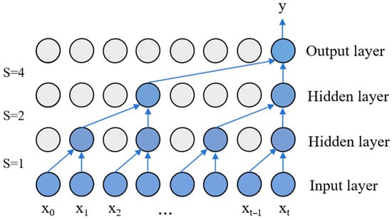
Figure 1. Expansion-causality convolution architecture diagram.

Simple causal convolutions struggle to process extended time series. To address this, TCN employs dilated convolutions. The computational process for dilated convolutions is as follows:

$$G(x_t)={\displaystyle {\displaystyle \sum }_{i=1}^{m-1}g(i)x_{t-si}}$$

(1)

where s denotes the expansion factor; g represents the filter; m indicates the filter size; g(i) signifies the i-th element of filter g; and G(x_t) denotes the network output corresponding to input x_t at time step t during the expansion convolution computation.

To address the vanishing or exploding gradient issues caused by introducing causal convolutions and dilated convolutions, TCN incorporates residual modules. These modules weight and fuse the model’s input x into its output G(x), ultimately yielding the TCN’s output y:

$$\mathrm{y}=Activation(x+G(x))$$

(2)

where Activation denotes the activation function; G(x) represents the output after the dilated convolution operation; and y signifies the final output of the residual module.

2.2. Informer

Informer is an enhanced high-performance prediction algorithm based on the Transformer architecture. It consists of an encoder and decoder, incorporating mechanisms such as multi-head probabilistic self-attention, self-attention distillation layers, and one-step forward prediction. It reduces computational complexity through multi-head sparse self-attention; addresses memory constraints caused by stacking lengthy sequences via self-attention distillation layers; and resolves slow prediction speeds for long sequences through one-step forward prediction. The Informer architecture is illustrated in Figure 2.

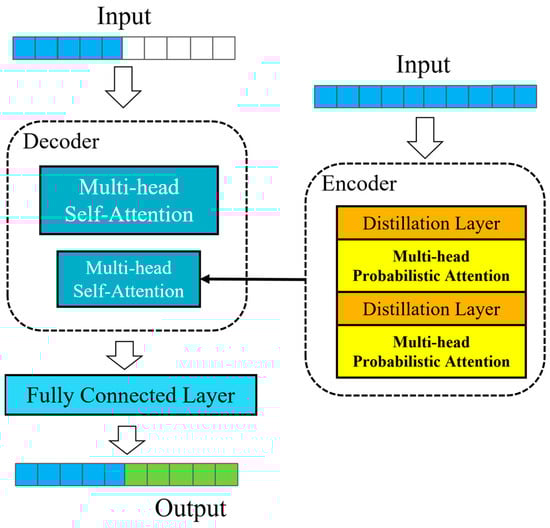
Figure 2. Structure of Informer.

In the Informer model: The encoder/decoder box-in-box module employs a stacked architecture, and multi-head probabilistic self-attention enhances the model’s capacity to recognize complex patterns in time series data. This is achieved by dividing the attention mechanism into multiple heads, thereby capturing contextual information across different subspaces within the input sequence. The self-attention distillation layer extracts knowledge from pre-trained self-attention models to improve learning efficiency and performance, particularly when parameters are limited or computational resources are scarce. One-step forward prediction enables the model to rapidly generate predictions for the next time step based on current information during time series forecasting, enhancing prediction immediacy and accuracy. For a comprehensive overview of the implementation procedures, please refer to reference [23].

3. Method

The proposed model utilizes a deep learning-based approach for wind speed prediction, with its framework illustrated in Figure 3. The fundamental premise of this model is the integration of historical meteorological data with terrain attributes derived from digital elevation models (DEMs), thereby facilitating precise wind speed predictions in complex topography through three key modules. First, a Topography-Aware Temporal Convolutional Network (T-TCN) extracts temporal evolution features of wind speed. Topographic information has been demonstrated to modulate the model’s initial weights, thereby enhancing its sensitivity to variations in wind speed. Secondly, a Topography-Spatial Bridging Unit (TSUB) integrates topographic features with meteorological data. The model incorporates relative position encoding, enabling it to comprehend spatial relationships between disparate geographic locations. The terrain-guided sparse attention mechanism (T-Informer) is a key component of the model, as it enables the model to focus on key terrain regions relevant to the prediction target when processing long-sequence data. This enhancement of prediction accuracy is a significant contribution of the T-Informer.

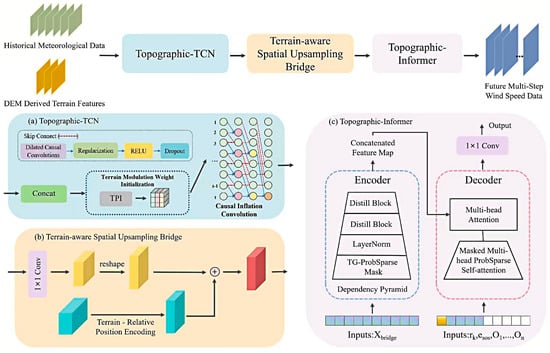
Figure 3. Algorithm framework.

3.1. T-TCN (Topographic-TCN)

In strong wind forecasting tasks, meteorological time series data exhibit significant short-term volatility and long-term dependencies. Recurrent neural networks (RNNs) and their variants, including long short-term memory (LSTM) and gated recurrent unit (GRU), encounter difficulties when explicitly incorporating static depth-of-field (DOF) information during the processing of meteorological data. To effectively capture multi-scale meteorological variability characteristics, this study extended this approach. Addressing the pronounced topographic forcing in strong wind processes over complex terrain, we propose the terrain-aware module T-TCN (Topographic-TCN). This module incorporates terrain attributes derived from digital elevation models (DEMs) as static covariates into the input layer. This enables the model to explicitly perceive terrain-modulated wind field processes while extracting temporal features.

Input tensors are concatenated using the “weather + terrain” approach:

$$X\in R^{T\times (D_{\mathrm{met}}+D_{dem})}$$

(3)

where T denotes the number of time steps, which is determined by the pre-event window length and sampling interval. Meteorological Channel Dmet = 6 (Air Temperature (°C), Air Pressure (hPa), Precipitation (mm), Wind Speed (m/s), Wind Direction (°), Humidity (%)) and the terrain channel D_dem = 3 (slope, aspect, and terrain position index TPI), which is bilinearly interpolated and resampled for each site and spatially and temporally aligned with meteorological sequences.

To enhance the model’s initial sensitivity to sudden wind signal changes in steep terrain areas, T-TCN employs a terrain-modulated weight initialization strategy. Building upon standard initialization, it applies a prior weighting to convolutional kernel weights using the site’s TPI value as a modulation factor:

$${\mathrm{w}}_k^{(l)}\leftarrow w_k^{(l)}\otimes (1+\alpha \cdot \tanh (TPI))$$

(4)

The modulation strength α = 0.1 was determined through grid search. This strategy enhances the response capability of channels corresponding to high TPI regions (such as ridges and passes) during the initial phase without altering the network structure, accelerating the convergence of precursor features for strong wind.

Each layer of the T-TCN transforms the input through a one-dimensional causal convolution. For each time step t, the causal convolution at layer L simultaneously operates on the joint meteorological-topographic channel:

$${\mathrm{h}}_t^{(\mathrm{l})}=\sigma ({\displaystyle {\displaystyle \sum }_{k=0}^{K-1}{W}_k^{(l)}}\cdot h_{t-d_l\cdot k}^{(l-1)}+b^{(l)})$$

(5)

where K denotes the convolution kernel size; d_l = 2^l−1 represents the dilation factor for layer L, which increases exponentially with depth; $W_{\mathrm{k}}^{(l)}\in R^{C_{out}\times C_{in}}$ represents learnable weights; σ(·) denotes the activation function; and causality is ensured by constraining t − d_l·k ≥ 0 to prevent the introduction of future information.

To stabilize training of deep networks, T-TCN incorporates residual connections. For layers with consistent channel counts, an identity mapping is performed:

$${\mathrm{h}}^{(t)}=\mathrm{Re}LU(Conv{D}_{causal,d_l}(h^{(l-1)}))+h^{(l-1)}$$

(6)

If the number of channels does not match, dimension alignment is performed via a 1 × 1 convolution:

$$h(l)=\mathrm{Re}LU(Conv1D_{causal,d_l}(h^{(l-1)}))+Conv1D_{1\times 1}(h^{(l-1)})$$

(7)

Ultimately, the T-TCN module outputs a high-dimensional temporal feature tensor after encoding:

$$Z=TCN(X)\in R^{T\times H},H=64$$

(8)

Among these, the hidden dimension H = 64 represents the optimal compromise point determined through grid search combined with early stopping. The feature tensor Z not only preserves the multiscale dynamic information of the original meteorological data sequence, but also integrates extensive temporal context through the dilated convolution mechanism. Simultaneously, it embeds terrain modulation information, providing the subsequent wind speed prediction module with an input representation that exhibits both physical consistency and terrain expressiveness.

3.2. TSUB (Terrain-Aware Spatial Upsampling Bridge)

The terrain-enhanced feature Z output by the T-TCN module contains local meteorological-terrain coupling information. However, its channel dimension does not match the dimension required by the subsequent Informer encoder and it lacks terrain-relative position priors. To address this, we designed a lightweight TSUB (Terrain-aware Spatial Upsampling Bridge) module to perform dimensionality expansion and inject terrain-relative position encoding, providing the Informer encoder with high-rank, terrain-sensitive input representations.

First, 1 × 1 pointwise convolution is applied to expand the 64-dimensional input to 512 dimensions:

$$X^{(0)}=Con{v}_{1\times 1}(Z)\in R^{24\times 512}$$

(9)

This operation does not alter the temporal resolution but merely reweights the T-TCN multiscale responses through cross-channel linear combinations, providing ample representational capacity for subsequent attention computations.

Since standard Transformers employ absolute cosine position encoding, they remain insensitive to non-uniform sampling (15-min intervals) and topographical variations. TSUB introduces learnable relative position encoding that simultaneously accounts for temporal lags and terrain-spatial differences:

$$P_{t,s}=w_r(\Delta t)+w\xi (\log d_{ij},\Delta h_{ij},\cos ({\mathrm{\Phi }}_i-{\mathrm{\Phi }}_j))$$

(10)

where $\Delta \mathrm{t}$ represents the time interval, d_ij denotes the horizontal distance between stations, h_ij indicates the elevation difference, and ${\mathrm{\Phi }}_{\mathrm{i}}$ represents the slope angle. The encoded vector is added element-wise to the features:

$$X^{(1)}=X^{(0)}+P$$

(11)

This enables the model to perceive typical terrain-lag modes such as “same slope-lag” or “leeward slope-synchronization” in subsequent attention computations without requiring additional parameters.

The TSUB module final output is

$$X_{\mathrm{bridge}}\in R^{T\times 512}$$

(12)

The temporal dimension is maintained at T steps while the channel dimension is expanded to 512, combining high-rank expressive power with terrain-relative position priors. This can be directly fed into the Informer encoder for subsequent global modeling.

3.3. T-Informer (Topographic-Informer)

Building upon the original Informer’s “encoder–decoder” framework, the T-Informer (Topographic-Informer) module was designed to optimize wind speed prediction over complex terrain by incorporating topographic prior information at each stage.

The input sequence length is designated as T = 20 for the T-Informer module encoder. The module is centered on Topographic-Guided ProbSparse Multi-head Self-attention (TG-ProbSparse Attention), which performs sparse filtering on masks under multi-head parallel processing. Subsequent to the output of 512-dimensional features, residual connections and LayerNorm have been demonstrated to stabilize training. Subsequently, a two-layer stacked Distillation block compresses sequence length, forming pyramid features E that incorporate both global dependencies and preserve topographically salient signals.

For input sequence X, a single distillation block performs

$$X_{\mathrm{out}}=MaxPool(ELU(Conv1D_{k-3}{,}_{causal}(X)))$$

(13)

Here, k denotes the causal convolution kernel size, causal represents causal convolution, and ELU signifies the activation function.

The decoder input is constructed using generative inference: first, a 512-dimensional learnable Start-of-Sequence embedding serves as the start token, followed by concatenation with an all-zero vector to form a future time slot placeholder. The learnable “terrain-wind type” vectors obtained from offline clustering are then concatenated by site type before the start token to form the decoder input. This step simultaneously injects terrain-wind prior information while reserving space for wind speed prediction. The decoder input construction is represented as follows:

$$X_{\mathrm{dec}}={\left[r_k,e_{sos},O_1,\dots ,O_n\right]}^T$$

(14)

where r_k denotes the learnable embedding for the k-th terrain-wind type; e_sos represents the learnable Start-of-Sequence vector; and O_t serves as a zero-padded placeholder at time step t.

The decoder self-attention employs a lower-triangular mask to prevent peeking at future observations. Cross-attention uses the encoder output E as the key/value, querying from the decoder itself to establish a historical-future mapping.

The decoder’s final hidden state D is reduced to a single channel via 1 × 1 convolution, yielding the wind speed prediction V_t:

$${\mathrm{V}}_{\mathrm{t}}=Con{v}_{1\times 1}(D_{-\mathrm{t}:})$$

(15)

where t denotes the result at the t-th time step; D_−t represents the hidden state after t time steps following the decoder output; and Conv_1×1 indicates a 1 × 1 convolution with an output channel of 1, mapping the 512-dimensional feature to a 1-dimensional wind speed value.

4. Experiment

4.1. Experimental Setup and Dataset

The experimental operating system environment used was Ubuntu 22.04, with an NVIDIA GeForce RTX 4070 12 GB graphics card, an AMD Ryzen 7 PRO 5845 CPU, and 16 GB of memory. The Python version used was 3.9.19, and the CUDA version was 12.4. The experiment ran for 500 iterations with a batch size of 20. Model training was optimized using the Adam optimizer with a learning rate of 5 × 10⁻⁴. The Adam optimizer’s exponential decay rates were set to 0.5 and 0.99, respectively, with an initial learning rate of 0.001.

This paper first selects the Wind Speed Prediction Dataset [24] to validate the model’s effectiveness in conventional wind speed prediction. The dataset covers convective conditions and includes daily average wind speed records from five meteorological variable sensors at weather stations, comprising 6574 samples as shown in Figure 4. Data originates from open areas and represents daily averages at a height of 21 m. The dataset includes scalar wind speed data (directionless), precipitation, maximum and minimum temperatures, and grass minimum temperature. This study utilizes four variables—wind speed, precipitation, maximum temperature, and minimum temperature—as model inputs. The dataset is partitioned into a training set (70% of total data), a test set (20% of total data), and a validation set (10% of total data).

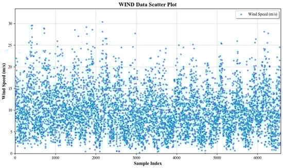
Figure 4. Daily wind speed sample sequences contained in the Wind Speed Prediction Dataset.

Secondly, this paper utilizes the SCWDS dataset from the China Meteorological Administration to validate the model’s effectiveness in strong wind forecasting [25]. This dataset is derived from severe convective weather records that have been meticulously archived by the National Meteorological Center of China. The records are sourced from 2413 national-level surface meteorological stations, thereby ensuring a comprehensive and representative sample of meteorological data. The study encompasses a total of 11,732 sample data points, which are distributed across a number of provinces, including Sichuan and Tibet. Figure 5 shows the number of events in each year, 2017–2024. The dataset under consideration encompasses 207 strong wind events, with each event providing hourly continuous observation sequences. Of these, 78.3% (165/207 events) occurred in complex terrain regions, encompassing the eastern edge of the Qinghai–Tibet Plateau and the Yunnan–Guizhou Plateau. The dataset encompasses scalar wind speed (directionless), air temperature, precipitation, atmospheric pressure, and humidity data corresponding to the time window of each strong wind event. The present study employs a model that incorporates five variables: wind speed, air temperature, precipitation, atmospheric pressure, and humidity. The spatial extent of the dataset was uniformly processed to 200 × 200 km. The temporal resolution employed event-driven sampling, with each sample recording the maximum 6-min wind speed within a 2-h window before and after severe convective events. This served as an operational proxy for short-duration strong winds. The dataset was partitioned into a training set, which comprised 70% of the total data, a test set, which comprised 20% of the total data, and a validation set, which comprised 10% of the total data.

Figure 5. The SCWDS dataset contains the number of daily wind speed observations. Data originate from national-level stations within a 200 km radius centered on the location of weather events, with wind speed measured at a height of 10 m.

This study evaluated the performance of predictive models using four metrics: Root Mean Square Error (RMSE), Mean Absolute Error (MAE), Mean Absolute Percentage Error (MAPE), and goodness-of-fit. Goodness-of-fit is commonly measured using the coefficient of determination (R-Square, R²). RMSE, MAE, and MAPE serve as accuracy assessment metrics, while R² functions as an indicator of the model’s goodness-of-fit.

(1) RMSE: A metric for measuring the magnitude of error between predicted and actual values. RMSE reflects the standard deviation of prediction errors; a smaller value indicates a higher model prediction accuracy.

$$RMSE=\sqrt{{\displaystyle \frac{1}{n}}{\displaystyle {{\displaystyle \sum }}_{i=1}^n{\left(y_i-{\widehat{y}}_i\right)}^2}}$$

(16)

Here, n denotes the sample size, y_i represents the i-th observed value (actual value), and i denotes the i-th predicted value.

(2) MAE: A measure of the average absolute deviation between predicted values and actual values. MAE provides the average absolute magnitude of prediction errors and is insensitive to outliers. A smaller value indicates a higher model prediction accuracy.

$$MAE={\displaystyle \frac{1}{n}}{\displaystyle {{\displaystyle \sum }}_{i=1}^n\left|y_i-{\widehat{y}}_i\right|}$$

(17)

(3) MAPE: A metric that measures the percentage of prediction error relative to the actual value. MAPE provides the percentage of prediction error relative to the actual value, with smaller values indicating higher prediction accuracy of the model.

$$MAPE={\displaystyle \frac{100\%}{n}}{\displaystyle {{\displaystyle \sum }}_{i=1}^n\left|\frac{y_i-{\widehat{y}}_i}{y_i}\right|}$$

(18)

(4) R²: A measure of how well a model explains the variation in the data. The closer the R² value is to 1, the better the model fits the data.

$$R^2=1-{\displaystyle \frac{{\displaystyle {{\displaystyle \sum }}_{i=1}^n{\left(y_i-{\widehat{y}}_i\right)}^2}}{{\displaystyle {{\displaystyle \sum }}_{i=1}^n{\left(y_i-{\overline{y}}_i\right)}^2}}}$$

(19)

Here, i represents the average value of the observed data.

4.2. Comparative Experiment on Conventional Wind Speed Prediction

In order to ascertain the efficacy of the model presented in this paper in predicting conventional wind speeds, a comparative experiment was conducted using the Wind Speed Prediction Dataset. It should be noted that the Wind Speed Prediction Dataset primarily originates from observational data under convective conditions. This implies that high wind speed events caused by non-convective factors (such as large-scale circulation systems and orographic acceleration) are underrepresented in the dataset. Given the current limited availability of publicly accessible wind speed prediction datasets, this dataset remains effective for validating the model’s predictive capability regarding conventional wind speed trends. In subsequent research, we will incorporate datasets encompassing more meteorological processes to further enhance the model’s universality.

This paper selects several widely used deep learning sequence prediction models as a control group, including Recurrent Neural Networks (RNN) [26], Long Short-Term Memory Networks (LSTM) [27], Bidirectional Long Short-Term Memory Networks (Bi-LSTM) [28], and Transformer models [29]. Furthermore, to comprehensively evaluate model performance, we also introduce several models that have demonstrated outstanding performance in wind speed sequence prediction: the Seq model [30], the SSA-BP model [31], and the GWO-BP model [32].

The experiment focuses on the daily forecasting cycle, employing RMSE, MAE, MAPE, and R² as quantitative metrics to evaluate the deviation between model predictions and actual values. In comparative experiments, we ensured all models were trained on identical training datasets. Input data underwent preprocessing via signal-frequency analysis methods such as Empirical Mode Decomposition (EMD) or Enhanced Empirical Mode Decomposition (EEMD). This approach enabled fair performance comparisons under consistent conditions, thereby validating the superiority of the proposed model.

In order to ascertain the reliability of the model’s wind speed prediction results, a total of 30 independent runs were conducted. The standard deviation of the prediction errors was subsequently calculated to determine the dispersion of the experimental results.

$$RMSE\sigma =\sqrt{{\displaystyle \frac{1}{N}}{{\displaystyle {\displaystyle \sum }_{i=1}^N(RMS{E}_i-\overline{RMSE})}}^2}$$

(20)

Within the formula, RMSEσ denotes the standard deviation of the 30 prediction errors, N represents the number of independent runs (30), RMSE_i indicates the root mean square error (RMSE) value of the ith independent run, and $\overline{RMSE}$ signifies the mean of the 30 RMSE values.

The p-value is a pivotal statistical parameter that is employed to ascertain the validity of predictive results. In this paper, the t-test is employed to assess significant differences among different models (with p < 0.05 as the significance level criterion).

The experimental results are presented in Table 1. The initial four columns present prediction evaluation metrics (RMSE, MAE, MAPE, R²), while the final two columns display robustness test metrics (σ, p). Among these, RMSE, MAE, R², and σ are all dimensionless statistics.

Table 1. Experimental Results Comparing Wind Speed Predictions Across Different Models on the Wind Speed Prediction Dataset.

Model	RMSE	MAE	MAPE	R2	RMSEσ	p
RNN	4.18	3.08	61.6%	0.73	0.02	<0.05
LSTM	4.06	2.94	58.8%	0.79	0.015	<0.05
Bi-LSTM	4.29	2.48	49.6%	0.84	0.018	<0.05
Transformer	3.47	2.80	56.0%	0.81	0.014	<0.05
Seq	2.19	2.71	54.6%	0.90	0.016	<0.05
GWO-BP	2.34	1.49	29.8%	0.88	0.018	<0.05
SSA-BP	1.79	1.37	27.4%	0.91	0.015	<0.05
Our	1.25	1.28	25.6%	0.95	0.008	<0.05

The Wind Speed Prediction Dataset for the input model comprises four variables: wind speed (m/s), maximum temperature (°C), minimum temperature (°C), and precipitation (mm). Due to the disparity in their numerical ranges and measurement units, direct input of these variables into the model would result in an uneven emphasis, amplifying the impact of variables with higher values in the prediction results while diminishing the influence of variables with lower values. Consequently, the raw variable data necessitates normalization processing.

The Z-score is a frequently employed technique for data normalization. Subsequent to the normalization process, the original variables entered into the model are converted into dimensionless values. This action aligns the variables on the same quantitative scale and facilitates the subsequent predictions of the model.

The formula for this substance is as follows:

Z = (x − μ)/σ

(21)

In this equation, x denotes the raw data value of the Wind Speed Prediction Dataset variable, μ represents the sample mean of this variable in the training set, and σ indicates the sample standard deviation of this variable in the training set.

Specifically, the model proposed in this paper achieved the lowest RMSE and MAE values of 1.25 and 1.28, respectively, indicating minimal error and the best predictive performance. Furthermore, it exhibited optimal MAPE performance at a mere 25.6%, denoting the lowest percentage error between predicted and actual values. Additionally, the model’s R² value of 0.95 approaches a perfect fit, thereby demonstrating its strongest ability to interpret data variations.

A comparison of the proposed model with RNN, LSTM, Bi-LSTM, and Transformer models reveals that the former attains optimal results across all evaluation metrics. In comparison to the Seq, SSA-BP, and GWO-BP algorithms, which have demonstrated efficacy in conventional wind speed forecasting, our model exhibits reduced errors in RMSE, MAE, and MAPE, while exhibiting enhanced fit in R². The findings suggest that the model exhibits enhanced accuracy and reliability in conventional wind speed prediction tasks.

To provide a more intuitive demonstration of the models’ predictive performance, this paper visualizes the wind speed prediction results of different models on the validation set, as shown in Figure 6.

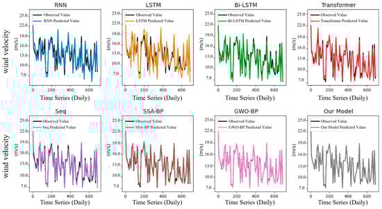
Figure 6. Performance of Different Models in Predicting Conventional Wind Speed on the Wind Speed Prediction Dataset.

The experimental findings suggest that the prediction curve of this model demonstrates the highest degree of alignment with the actual value curve, exhibiting minimal deviation and error. This finding suggests that the model exhibits a notable advantage in predicting conventional wind speeds. Furthermore, the GWO-BP and SSA-BP algorithms demonstrate satisfactory predictive performance, with their prediction curves closely approximating the actual value curve. In contrast, deep learning-based models, such as RNN and LSTM, while demonstrating the capacity to discern the general trend of wind speeds, exhibit reduced prediction accuracy in specific regions when compared to the custom model and alternative optimization algorithms.

4.3. Strong Wind Forecast Comparison Experiment

The present study utilizes the SCWDS dataset to conduct comparative experiments on strong wind forecasting, with the objective of evaluating the model’s predictive performance. In order to more accurately assess the model’s capability in strong wind prediction, this section of comparative experiments abandons metrics such as MAE and instead utilizes the following indicators to evaluate the model’s forecasting performance:

(1) Accuracy

Accuracy refers to the proportion of correctly predicted samples out of the total number of samples. It is a commonly used performance metric for measuring the overall predictive accuracy of a model, the higher the value, the higher the model’s prediction accuracy. The calculation formula is as follows:

$$Accuracy={\displaystyle \frac{TP+TN}{TP+TN+FP+FN}}$$

(22)

where TP represents true positives (correctly predicted positive cases), TN denotes true negatives (correctly predicted negative cases), FP signifies false positives (incorrectly predicted positive cases), and FN indicates false negatives (incorrectly predicted negative cases).

(2) True Skill (TS) Score

TS score is a metric that comprehensively evaluates both true positives and true negatives, measuring the usefulness of a model’s predictions, the smaller the value, the higher the model’s prediction accuracy. The calculation formula is as follows:

$$TS={\displaystyle \frac{TP}{TP+FP+FN}}$$

(23)

The higher the TS score, the better the model performs in predicting extreme events.

(3) Miss Rate (MR)

The miss rate refers to the proportion of actual extreme events that the model fails to correctly predict. The calculation formula is as follows:

$$MR={\displaystyle \frac{FN}{TP+FN}}$$

(24)

The lower the false negative rate, the higher the predictive accuracy of the model.

(4) False Alarm Rate (FAR)

The false alarm rate refers to the proportion of non-extreme events that the model incorrectly predicts as extreme events. The calculation formula is as follows:

$$FAR={\displaystyle \frac{FP}{TN+FP}}$$

(25)

The lower the false alarm rate, the higher the predictive accuracy of the model.

The comparison algorithms employed in this experiment represent state-of-the-art artificial intelligence models, demonstrating strong performance in wind speed prediction. The following models are of particular significance: RNN, LSTM, Transformer, Bi-LSTM, PredRNN, as well as the advanced wind speed prediction algorithms MAU [33] and STAM [34].

The comparative experiment utilized five variables from the SCWDS dataset—wind speed, air temperature, precipitation, air pressure, and humidity—combined with three regional variables: slope gradient, slope aspect, and terrain position index (TPI) as model inputs. The prediction results were uniformly defined as follows: values ≥17 m/s were classified as “1,” while values <17 m/s were classified as “0.” The comparative results of strong wind predictions across different models using the SCWDS dataset are presented in Table 2.

Table 2. Comparison of Extreme Wind Prediction Results Across Different Models on the SCWDS Dataset.

Model	$\mathbf{A}\mathbf{c}\mathbf{c}\mathbf{u}\mathbf{r}\mathbf{a}\mathbf{c}\mathbf{y}$	TS Score	MR	FAR
RNN	0.28	0.35	52.4%	27.6%
LSTM	0.34	0.24	54.6%	25.4%
Transformer	0.21	0.16	51.7%	19.1%
Bi-LSTM	0.55	0.33	50.9%	18.4%
PredRNN	0.47	0.29	47.6%	16.9%
MAU	0.51	0.41	49.0%	16.1%
STAM	0.62	0.45	35.5%	15.3%
Our	0.70	0.57	34.2%	10.6%

The experimental results indicate that the proposed model attained the highest scores in Accuracy and TS Score, specifically 0.70 and 0.57, respectively, substantiating its remarkable accuracy in predicting strong wind events. The proposed model demonstrates superiority in MR and FAR metrics, with underreporting and overreporting rates of 24.2% and 10.6%, respectively—values that are considerably lower than those observed in other comparison methods. In contrast, Bi-LSTM exhibits underreporting and overreporting rates of 50.9% and 18.4%, respectively, while Transformer shows rates of 51.7% and 19.1%.

Meanwhile, the STAM model demonstrated somewhat poorer performance in experiments, validating the effectiveness of its spatio-temporal attention mechanism. However, our model achieved a 26.7% improvement in TS score compared to STAM, while reducing the false negative rate and false positive rate by 31.8% and 30.7%, respectively. This improvement stems from the terrain-guided sparse attention mechanism’s precise focusing capability on complex topographical features such as ridges and passes. Furthermore, while STAM employs purely data-driven attention, the proposed model demonstrates superior generalization by incorporating relevant terrain data. Experimental results indicate that the proposed model achieves higher reliability and accuracy in strong wind prediction.

The model presented in this paper demonstrates superior performance across all four evaluation metrics: Accuracy, TS Score, FAR, and FAR. This indicates the model’s capacity to predict strong winds with greater accuracy and reliability. These performance enhancements are attributable to the model’s innovative physical mechanisms, which primarily encompass the following aspects:

(1) Terrain-Modulated Initialization: By pre-weighting convolutional kernel weights using the Terrain Position Index (TPI), the model responds more sensitively to wind speed variations in terrain-sensitive regions such as ridges and valleys. This terrain-modulation mechanism enables the model to better capture terrain’s accelerating, decelerating, and guiding effects on wind speed, thereby enhancing its predictive capability for extreme wind events.

(2) Terrain-Relative Position Encoding: The TSUB module introduces terrain-relative position encoding, injecting terrain variations and spatial relative position information into the feature space. This encoding mechanism enables the model to better perceive terrain’s influence on wind speed variations, significantly improving prediction accuracy, particularly in complex terrain.

(3) Terrain-Guided Sparse Attention: The T-Informer module employs terrain-guided sparse attention to dynamically adjust attention weight distributions, enabling the model to focus on terrain-sensitive regions. This attention mechanism excels in handling extreme wind events, substantially reducing both under-reporting and over-reporting rates.

The aforementioned aspects illustrate that the model presented in this paper possesses significant advantages in capturing strong wind events, which is crucial for its further practical application in strong wind warning systems.

5. Conclusions

The present study proposes a deep learning algorithm for predicting wind speeds in complex terrain based on meteorological data, with the objective of achieving precise wind speed predictions. First, by incorporating terrain-related data and designing a weight initialization strategy, higher response weights are assigned to terrain-complex regions at the input stage. Secondly, by incorporating terrain-relative position priors into the high-dimensional feature space, the efficient coupling of local abrupt features with global structural information is facilitated. In conclusion, the model’s precision in forecasting strong winds is significantly enhanced by the terrain-guided sparse attention mechanism. The model’s capability for routine wind speed prediction was validated through experimental means. To this end, daily observations from the Wind Speed Prediction Dataset were utilized, while its performance in forecasting strong wind events was assessed using continuous observations from the SCWDS dataset. Of the models tested, experimental findings indicate that the proposed model attains optimal prediction outcomes for both conventional wind speeds and strong wind events, manifesting significant advantages of high accuracy and low false alarm rates. Subsequent research endeavors will concentrate on the following areas: First, multimodal observational data is introduced to explore a fusion prediction framework driven by radar-satellite-ground station collaboration. Second, conducting cross-regional transfer experiments is necessary to validate the model’s applicability and stability across different topographic and climatic zones, such as the Qinghai–Tibet Plateau and the southeastern coastal regions.

References

- Gao, Y.; Zeng, F. Value-Added Areas and Implementation Pathways for Synergistic Development of Meteorology and the “Dual Carbon” Strategy. Product. Res. 2024, 28, 30–35. [Google Scholar]
- Liu, H.; Mi, X.; Li, Y. Smart deep learning based wind speed prediction model using wavelet packet decomposition, convolutional neural network and convolutional long short term memory network. Energy Convers. Manag. 2018, 166, 120–131. [Google Scholar] [CrossRef]
- China Meteorological Administration. Specifications for Surface Meteorological Observation; China Meteorological Press: Beijing, China, 2003. [Google Scholar]
- Gazafroudi, A.S. Assessing the Impact of Load and Renewable Energies’ Uncertainty on a Hybrid System. Int. J. Energy Power Eng. 2016, 5, 2016050202-11. [Google Scholar] [CrossRef]
- Huang, Y.; Zhang, B.; Pang, H.; Wang, B.; Lee, K.Y.; Xie, J.; Jin, Y. Spatio-temporal wind speed prediction based on Clayton Copula function with deep learning fusion. Renew. Energy 2022, 192, 526–536. [Google Scholar] [CrossRef]
- Ding, Y.; Ye, X.W.; Guo, Y. A multistep direct and indirect strategy for predicting wind direction based on the EMD-LSTM model. Struct. Control Health Monit. 2023, 2023, 4950487. [Google Scholar] [CrossRef]
- Li, X.; Li, K.; Shen, S.; Tian, Y. Exploring time series models for wind speed forecasting: A comparative analysis. Energies 2023, 16, 7785. [Google Scholar] [CrossRef]
- Valdivia-Bautista, S.M.; Domínguez-Navarro, J.A.; Pérez-Cisneros, M.; Vega-Gómez, C.J.; Castillo-Téllez, B. Artificial intelligence in wind speed forecasting: A review. Energies 2023, 16, 2457. [Google Scholar] [CrossRef]
- Khan, S.; Mazhar, T.; Khan, M.A.; Shahzad, T.; Ahmad, W.; Bibi, A.; Saeed, M.M.; Hamam, H. Comparative analysis of deep neural network architectures for renewable energy forecasting: Enhancing accuracy with meteorological and time-based features. Discov. Sustain. 2024, 5, 533. [Google Scholar] [CrossRef]
- Shao, B.; Song, D.; Bian, G.; Zhao, Y. Wind speed forecast based on the LSTM neural network optimized by the firework algorithm. Adv. Mater. Sci. Eng. 2021, 2021, 4874757. [Google Scholar] [CrossRef]
- Wang, M.; Wang, J.; Yu, M.; Yang, F. Spatiotemporal wind speed forecasting using conditional local convolution and multidimensional meteorology features. Sci. Rep. 2024, 14, 26219. [Google Scholar] [CrossRef] [PubMed]
- Yu, C.; Ma, Y. A novel model for wind speed point prediction and quantifying uncertainty in wind farms. Electr. Eng. 2025, 107, 6395–6409. [Google Scholar] [CrossRef]
- Ma, J.; Liu, W.; Yan, W. Deep Learning-Based Methods for Meteorological Element Prediction. J. Trop. Meteorol. 2021, 37, 186–193. [Google Scholar] [CrossRef]
- Liang, T.; Chen, C.; Tan, J.; Jing, Y. Wind Speed Prediction Based on Multi-aspect Feature Extraction and Transfer Learning. J. Sol. Energy 2023, 44, 132–139. [Google Scholar]
- Niu, Z.; Yu, Z.; Tang, W.; Wu, Q.; Reformat, M. Wind power forecasting using attention-based gated recurrent unit network. Energy 2020, 196, 117081. [Google Scholar] [CrossRef]
- Khattak, A.; Zhang, J.; Chan, P.-W.; Chen, F. Assessment of wind shear severity in airport runway vicinity using interpretable TabNet approach and Doppler LiDAR data. Appl. Artif. Intell. 2024, 38, 2302227. [Google Scholar] [CrossRef]
- Hu, F.; Feng, X.; Xu, H.; Liang, X.; Wang, X. Ultra-short-term spatio-temporal wind speed prediction based on OWT-STGradRAM. IEEE Trans. Sustain. Energy 2025, 16, 1–18. [Google Scholar] [CrossRef]
- Zhang, Z.; Lin, L.; Gao, S.; Wang, J.; Zhao, H.; Yu, H. A machine learning model for hub-height short-term wind speed prediction. Nat. Commun. 2025, 16, 3195. [Google Scholar] [CrossRef]
- Dujardin, J.; Lehning, M. Wind-Topo: Downscaling near-surface wind fields to high-resolution topography in highly complex terrain with deep learning. Q. J. R. Meteorol. Soc. 2022, 148, 1368–1388. [Google Scholar] [CrossRef]
- Le Toumelin, L.; Gouttevin, I.; Galiez, C.; Helbig, N. A two-fold deep-learning strategy to correct and downscale winds over mountains. Nonlinear Process. Geophys. 2024, 31, 75–97. [Google Scholar] [CrossRef]
- Liu, J.; Shi, C.; Ge, L.; Tie, R.; Chen, X.; Zhou, T.; Gu, X.; Shen, Z. Enhanced wind field spatial downscaling method using UNET architecture and dual cross-attention mechanism. Remote Sens. 2024, 16, 1867. [Google Scholar] [CrossRef]
- Li, Y.; Zhang, L.; Lei, Y.; Ran, J.; Ye, G. Short-term electricity consumption forecasting method based on temporal convolutional network and gated re-current unit. Water Resour. Power 2021, 39, 198–201. [Google Scholar]
- Zhou, H.; Zhang, S.; Peng, J.; Zhang, S.; Li, J.; Xiong, H.; Zhang, W. Informer: Beyond efficient transformer for long sequence time-series forecasting. In Proceedings of the AAAI Conference on Artificial Intelligence, Virtual, 2–9 February 2021; Volume 35, pp. 11106–11115. [Google Scholar]
- Fedesoriano. “Wind Speed Prediction Dataset”. Kaggle, 2022. Available online: https://www.kaggle.com/datasets/fedesoriano/wind-speed-prediction-dataset (accessed on 10 July 2025).
- Liu, N.; Xiong, A.; Zhang, Q.; Liu, Y.; Zhan, Y.; Liu, Y. Construction of a Basic Dataset for Training Artificial Intelligence Applications in Severe Convective Weather. J. Appl. Meteorol. 2021, 32, 530–541. [Google Scholar] [CrossRef]
- Medsker, L.R.; Jain, L. Recurrent neural networks. Des. Appl. 2001, 5, 2. [Google Scholar]
- Hochreiter, S.; Schmidhuber, J. Long short-term memory. Neural Comput. 1997, 9, 1735–1780. [Google Scholar] [CrossRef]
- Wang, S.; Wang, X.; Wang, S.; Wang, D. Bi-directional long short-term memory method based on attention mechanism and rolling update for short-term load forecasting. Int. J. Electr. Power Energy Syst. 2019, 109, 470–479. [Google Scholar] [CrossRef]
- Vaswani, A.; Shazeer, N.; Parmar, N.; Uszkoreit, J.; Jones, L.; Gomez, A.N.; Kaiser, Ł.; Polosukhin, I. Attention is all you need. arXiv 2017, arXiv:1508.04409. [Google Scholar] [CrossRef]
- Du, B.; Li, Y.; Ma, Z.; Wang, H.; Zhang, L. A Seq2Seq Wind Speed Prediction Model with Multi-Feature Embedding. Comput. Eng. Des. 2021, 42, 2061–2068. [Google Scholar]
- Zhang, J.; Meng, J.; Li, D.; Chen, X. Wind Speed Prediction Method Along Railway Lines Based on SSA-BP. Comput. Simul. 2023, 40, 209–212+260. [Google Scholar]
- Wang, Y.; Wang, X.; Duan, Y. Short-Term Wind Power Generation Forecasting Based on the GWO-BP Model. Yunnan Hydropower 2023, 39, 67–71. [Google Scholar]
- Chang, Z.; Zhang, X.; Wang, S.; Ma, S.; Ye, Y.; Xiang, X.; Gao, W. MAU: A motion-aware unit for video prediction and beyond. Adv. Neural Inf. Process. Syst. 2021, 34, 26950–26962. [Google Scholar]
- Chang, Z.; Zhang, X.; Wang, S.; Ma, S.; Gao, W. STAM: A spatiotemporal attention based memory for video prediction. IEEE Trans. Multimed. 2022, 25, 2354–2367. [Google Scholar] [CrossRef]
Disclaimer/Publisher’s Note: The statements, opinions and data contained in all publications are solely those of the individual author(s) and contributor(s) and not of MDPI and/or the editor(s). MDPI and/or the editor(s) disclaim responsibility for any injury to people or property resulting from any ideas, methods, instructions or products referred to in the content. |
© 2025 by the authors. Licensee MDPI, Basel, Switzerland. This article is an open access article distributed under the terms and conditions of the Creative Commons Attribution (CC BY) license.