Real-Time Production of High-Resolution, Gap-Free, 3-Hourly AOD over South Korea: A Machine Learning Approach Using Model Forecasts, Satellite Products, and Air Quality Data

Abstract

Aerosol optical depth (AOD) is essential for air quality monitoring and climate research. However, satellite-based retrievals suffer from cloud-related data gaps, and reanalysis products are limited by coarse spatial resolution and substantial production latency. This study develops a real-time, gap-free, high-resolution (1.5 km) AOD retrieval system for South Korea. The system integrates Copernicus Atmosphere Monitoring Service (CAMS) forecasts, high-resolution meteorological fields, and ground-based air quality observations within a machine learning framework. Three models with varying training periods were systematically evaluated using cross-validation and independent validation with 2024 Aerosol Robotic Network (AERONET) data. The optimal model, trained on 2015–2023 data, achieved a mean absolute error (MAE) of 0.075 and a correlation coefficient (R) of 0.841 during the 2024 independent validation, significantly outperforming the original CAMS forecast. The system demonstrated robust and consistent performance across varying land cover types, seasons, and AOD conditions, from clean to highly polluted. Empirical orthogonal function (EOF) analysis confirmed that the product successfully captures physically meaningful spatiotemporal patterns, including transboundary pollution transport, regional emission gradients, and topographic effects. Providing real-time, gap-free, 3-hourly daytime AOD, the proposed model overcomes the limitations of cloud-induced gaps in satellite data and the latency and coarseness of reanalysis products. This enables robust operational monitoring and aerosol research across the Korean Peninsula.

1. Introduction

Atmospheric aerosols are fine solid or liquid particles suspended in the atmosphere that exert diverse impacts on the Earth system, including radiative forcing and climate processes [1,2]. These particles, emitted into the atmosphere through natural processes (e.g., sea salt, wildfires, and volcanic ash) and anthropogenic activities (e.g., fossil fuel combustion), serve as both key variables in climate change and major air pollutants that determine air quality [3]. To quantify and monitor the complex effects of aerosols, various parameters are employed, among which the most fundamental is the Aerosol Optical Depth (AOD). AOD is a dimensionless quantity that represents the degree to which solar radiation is attenuated by scattering and absorption caused by aerosols along the entire vertical atmospheric column. Because it quantifies the total aerosol loading in the atmosphere and reflects regional air pollution levels and characteristics, AOD has been widely used in atmospheric monitoring studies, facilitated by its capability for both ground-based and satellite-based remote sensing [4,5].

To accurately monitor aerosol properties, National Aeronautics and Space Administration (NASA) developed the Aerosol Robotic Network (AERONET) system—an international federation of ground-based sun/sky radiometer networks operating globally [6]. Through standardized instrumentation and rigorous quality control protocols, AERONET ensures high accuracy and consistency in AOD measurements across stations worldwide, making it a global benchmark dataset for validation in numerous studies [7,8,9,10]. While AERONET provides high temporal resolution and accuracy at specific sites, its spatial coverage remains limited, making it challenging to capture spatiotemporal variability of aerosol. Therefore, for spatially continuous and long-term aerosol characterization, satellite- and model-based AOD products are indispensable.

Satellite sensors such as the Moderate Resolution Imaging Spectroradiometer (MODIS), Visible Infrared Imaging Radiometer Suite (VIIRS), and Multi-Angle Imaging Spectroradiometer (MISR) have provided long-term, global AOD raster datasets [11,12]. These products form the foundation for studies of long-range aerosol transport, air quality trends, and climate model evaluation at global scales. However, the most significant obstacle to satellite-based AOD retrieval is cloud contamination, which causes large areas of missing data. Moreover, undetected sub-pixel clouds or cloud shadows can be misinterpreted as high-concentration aerosol plumes, leading retrieval algorithms to overestimate AOD [13] severely.

In contrast, model-based AOD is derived from numerical models that simulate aerosol generation, transport, and removal processes using physical and chemical equations, combined with satellite and ground-based observations through data assimilation systems. Systems such as Copernicus Atmosphere Monitoring Service (CAMS) and Modern-Era Retrospective Analysis for Research and Applications Version 2 (MERRA-2) compensate for missing satellite data and provide spatially and temporally continuous, physically consistent aerosol datasets [14,15]. Data assimilation enhances the accuracy of reanalysis products compared with standalone numerical models and supports future air quality forecasting. However, the coarse spatial resolution (tens of kilometers) imposed by computational constraints hinders the representation of local-scale phenomena. Furthermore, uncertainties originating from emission inventories, boundary conditions, and parameter approximations can introduce systematic biases [16,17,18]. According to the CAMS global reanalysis validation report, CAMS tends to underestimate AOD over major dust source regions such as the Sahara Desert and exhibits regional biases due to inadequate representation of biomass-burning and secondary organic aerosol optical properties [19].

Recently, artificial intelligence (AI) techniques such as machine learning (ML) and deep learning (DL) have emerged as powerful tools for AOD estimation, leveraging their ability to learn complex and nonlinear relationships utilizing large datasets of auxiliary variables. For instance, Lipponen et al. [20] applied a deep learning correction network to predict the approximation error between Sentinel-3 AOD products and AERONET observations, achieving accuracy improvements compared with the original product. She et al. [21] proposed a deep neural network (DNN) model that directly retrieves AOD from Himawari-8 top-of-atmosphere (TOA) reflectance, demonstrating that AOD estimation can be achieved directly from satellite reflectance without inverse correction. To address spatial data gaps in satellite observations, Liu et al. [22] developed a Bi-ConvRNN model that combines convolutional neural networks (CNNs) and bidirectional recurrent neural networks (RNNs) to fill hourly gaps in Geostationary Ocean Color Imager (GOCI) AOD data. Ding et al. [23] integrated MODIS Multi-Angle Implementation of Atmospheric Correction (MAIAC) and MERRA-2 AOD products using a TabNet model to generate a daily 0.01° gap-free AOD dataset for Asia with the Root Mean Square Error (RMSE) of 0.23.

These studies have demonstrated achievements in enhancing retrieval accuracy, learning complex nonlinear relationships, filling spatial gaps, and correcting systematic biases. Nevertheless, each has its own drawbacks, which depend on limited objectives and methodologies. Satellite-based approaches provide high temporal resolution; however, significant challenges remain due to missing pixels caused by clouds and other surface reflectance issues. While studies supplementing these satellite gaps with reanalysis data have shown excellent performance, their real-time applicability is limited by production delays of several months. Moreover, because satellite AOD is typically used as a regression target, retrieval accuracy cannot exceed that of the original satellite data [22]. Efforts to improve reanalysis accuracy have generally been conducted at a daily temporal resolution, meaning their outputs cannot reflect the diurnal variation of AOD.

Therefore, this study aims to develop a real-time AOD retrieval system that provides high-resolution, gap-free, 3-hourly data over South Korea. This is achieved by combining CAMS AOD forecasts, satellite AOD climatology, meteorological data, and air quality data within a machine learning framework. The resulting outputs demonstrate the highest accuracy among similar studies, irrespective of season and land cover type, allowing for its practical application to real-time AOD monitoring. Furthermore, the Empirical Orthogonal Function (EOF) analysis is employed to reveal the spatiotemporal variability of the AOD field over South Korea.

2. Materials and Methods

2.1. Study Region

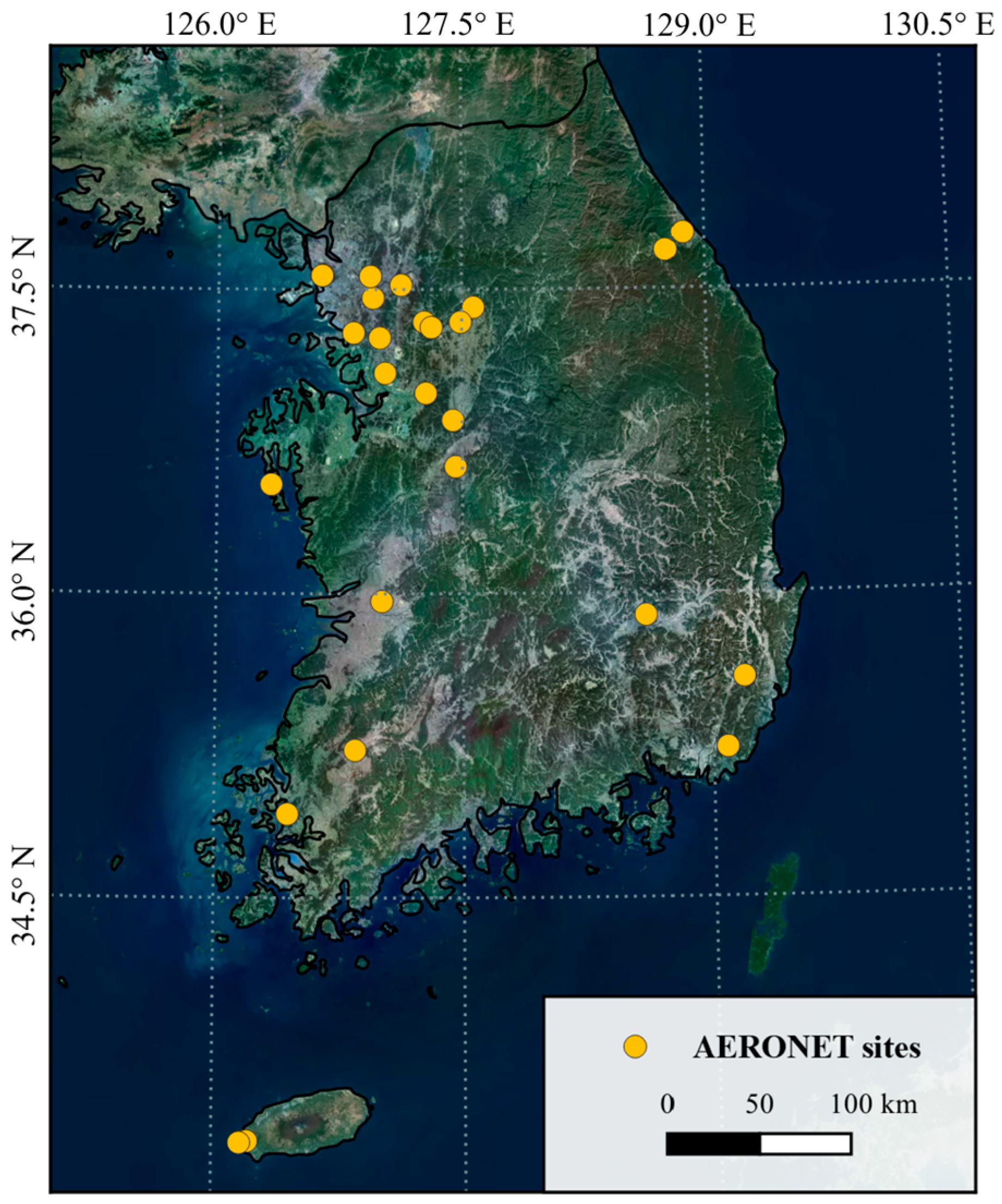
The Korean Peninsula, located along the eastern margin of the East Asian continent, is influenced by both long-range transboundary transport from China and local anthropogenic emissions, resulting in pronounced spatiotemporal variability in aerosol concentrations [24,25]. In particular, the combined effects of springtime Asian dust events and regional air pollution highlight the need for high spatial and temporal resolution AOD monitoring. Moreover, Korea’s complex topography (comprising mountains, plains, and coastal regions) and the complex terrain and land surface within its relatively small territory pose challenges for accurate representation when using coarse-resolution CAMS data (approximately 0.4°). Frequent cloud occurrences further hinder the spatiotemporal continuity of satellite observations. To overcome these limitations, we focused on the terrestrial regions of Korea to develop a high-resolution, gap-free, 3-hourly AOD retrieval system, for daytime periods when AOD observations are typically available (Figure 1).

Figure 1. Location of South Korea and distribution of inland AERONET sites (n = 26, yellow dots).

2.2. Datasets

2.2.1. AERONET AOD

AERONET is a global ground-based sun photometer network operated under the leadership of NASA’s Goddard Space Flight Center, providing optical and physical aerosol property measurements, including AOD [6]. The AERONET observations exhibit relative uncertainties of 0.2–0.5% for reference instruments and about 1.5% for field instruments in the visible and near-infrared spectral ranges [26]. AERONET Version 3 classifies its data by quality level as Level 1.0 (unscreened), Level 1.5 (cloud-screened), and Level 2.0 (quality-assured). Level 2.0 represents the final quality-assured dataset corrected before and after field deployment, with an accuracy of ±0.01–0.02 for wavelengths ranging from 340 to 1640 nm [27]. We used observations from 26 AERONET stations across inland Korea, as illustrated in Figure 1 and detailed in Appendix A. The quality-assured AOD measurements from 2015 to 2024 were used as ground truth reference data for our AI modeling.

2.2.2. AOD Forecast Field

The CAMS, operated by the European Centre for Medium-Range Weather Forecasts (ECMWF), provides atmospheric monitoring and forecasting services by integrating numerical modeling, satellite observations, and in situ measurements. CAMS issues global atmospheric composition forecasts twice daily (00 and 12 UTC) at approximately 40 km × 40 km resolution, predicting the spatiotemporal distributions of aerosols and trace gases on a real-time basis. The CAMS global atmospheric composition forecasting system is based on the Integrated Forecasting System (IFS). It assimilates satellite-derived AOD data from MODIS, VIIRS, and Polar Multi-Sensor Aerosol Product (PMAP) through four-dimensional variational data assimilation (4D-VAR). We used the Total Aerosol Optical Depth at 550 nm product from 2015 to 2024. Because this dataset does not incorporate ground-based measurements such as AERONET observations into its assimilation process [28], it can be used as an input variable for our AI modeling. Validation of CAMS AOD forecasts over East Asia for March–May 2025 shows a correlation coefficient (R) of 0.72 with AERONET observations [29], indicating that the model provides reliable synoptic-scale aerosol information.

2.2.3. Monthly AOD Climatology

The MODIS onboard the Terra and Aqua satellites employ the MAIAC algorithm, which integrates time-series analysis and image processing for cloud detection, aerosol retrieval, and atmospheric correction [30]. We used MODIS MAIAC AOD data at 550 nm with approximately 1 km spatial resolution to generate a monthly AOD climatology over the past 20 years (2004–2023). daily MAIAC AOD over South Korea has been validated against AERONET with R = 0.836 [31], confirming its reliability. While daily MAIAC AOD is ideal for capturing day-to-day variability, it often contains significant spatial gaps due to cloud cover, limiting its utility for real-time operational applications. To ensure spatiotemporally continuous AOD estimates at 3-hourly intervals, we utilized meteorological variables at a 3-hourly resolution. Furthermore, daily MAIAC AOD was aggregated monthly to provide a spatio-seasonal baseline, allowing the model to more effectively distinguish anomalous deviations from expected background conditions. The climatology provides the “expected” background, while the other dynamic predictors provide the “signal” for extreme episodes.

2.2.4. Numerical Model-Based Meteorological Data

Gridded meteorological data were obtained in real time from the Local Data Assimilation and Prediction System (LDAPS) operated by the Korea Meteorological Administration (KMA). LDAPS is a regional forecasting system based on the Unified Model (UM) that provides high-resolution (1.5 km) meteorological forecasts over the Korean Peninsula. The system receives boundary conditions from a global model at 3-h intervals and produces eight forecasts per day (00, 03, 06, 09, 12, 15, 18, and 21 UTC). We used analysis fields at 00, 03, 06, and 09 UTC as meteorological inputs.

A total of 11 meteorological parameters were used for AOD retrieval, grouped into four categories: moisture, dynamics, precipitation, and radiation. Moisture-related variables (specific humidity, relative humidity, dew point temperature, latent heat flux, and low cloud cover: RH, DPT, LHTFL, and LCDC) govern hygroscopic growth of aerosols. Under high relative humidity conditions, aerosol light scattering increases nonlinearly, substantially enhancing AOD [32,33]. Dynamic variables (wind components and planetary boundary layer height: UGRD, VGRD, and HPBL) determine aerosol transport, dispersion, and vertical dilution. Shallow boundary layers promote aerosol accumulation near the surface, thereby elevating AOD. Temperature (TMP) and pressure (PRES) influence atmospheric stability and indirectly modulate boundary layer height [34,35,36]. Precipitation-related variables (convective precipitation and low cloud cover: NCPCP and LCDC) represent wet scavenging processes that remove aerosols from the atmosphere, reducing AOD [37]. Finally, the radiative variable (total downward shortwave radiation: TDSWR) reflects solar attenuation by aerosols and associated surface cooling effects [38]. According to the 2024 KMA verification report, LDAPS achieves 24-h forecast RMSE values of 1.59 °C for 850 hPa temperature and 12.18 m for 500 hPa geopotential height over South Korea [39]. These metrics demonstrate its high fidelity in representing the meteorological forcing required for aerosol modeling.

2.2.5. Ground-Based Air Quality and Meteorological Data

Ground-based air quality data were obtained from the AirKorea network operated by the Korea Ministry of Climate, Energy and Environment, which provides real-time pollutant concentrations from 663 monitoring stations nationwide. The stations measure four gaseous species (sulfur dioxide, carbon monoxide, nitrogen dioxide, and ozone; SO₂, CO, NO₂, O₃) and two species of particulate matter (PM), such as PM10 and PM2.5, in accordance with national ambient air quality monitoring standards.

PM includes not only primary particles directly emitted from sources, but also secondary particles formed when gaseous precursors such as SO₂, nitrogen oxides (NO_X), and volatile organic compounds (VOCs) undergo chemical reactions under specific meteorological conditions to produce sulfates (SO_X) and other secondary aerosols [40,41,42]. These gaseous precursors and particulate concentrations directly influence AOD by scattering and absorbing visible radiation. Consequently, all six pollutant variables were employed as inputs for our AI modeling.

Additionally, the Korea Meteorological Administration operates the Automated Synoptic Observing System (ASOS), which provides visibility observations from 95 stations nationwide. Visibility data is derived from laser beam scattering intensity and reported as a 10-min moving average. Because visibility directly reflects the optical properties of atmospheric particles and is closely related to AOD, ASOS visibility data were incorporated as an additional input variable to enhance AOD retrieval performance.

Table 1 summarizes the datasets used in this study. While AERONET AOD serves as the target variable, the remaining 20 variables are the input features selected following a redundancy analysis.

Table 1. The data information used in this study.

Datasets	Parameter	Description	Resolution
AERONET AOD	AOD_500 nm	AOD at 500 nm
	440–675_Angstrom_Exponent	Ångström Exponent (440–675 nm)
CAMS AOD	Total aerosol optical depth at 550 nm	AOD at 550 nm	40 km/1 h
MAIAC AOD	AOD_550 nm	AOD at 550 nm	1 km/1 day
LDAPS	TDSWS	Total Downward Surface Shortwave Flux	1.5 km/3 h
	NCPCP	Large-Scale Precipitation
	UGRD	U-Component of Wind
	VGRD	V-Component of Wind
	LHTFL	Latent Heat Net Flux
	TMP	Temperature
	RH	Relative Humidity
	DPT	Dew Point Temperature
	LCDC	Low Cloud Cover
	HPBL	Planetary Boundary Layer Height
	PRES	Surface Pressure
AirKorea	SO2	Sulfur Dioxide (SO2)	1 h
	CO	Carbon Monoxide
	NO2	Nitrogen Dioxide (NO2)
	O3	Ozone (O3)
	PM10	Particulate Matter ≤ 10 μm
	PM2.5	Particulate Matter ≤ 2.5 μm
KMA ASOS	VIS	Visibility	1 h

2.3. Data Processing and Integration

2.3.1. Data Preprocessing

The matching between CAMS AOD and AERONET observations was performed by extracting, for each hour (00, 03, 06, and 09 UTC), the nearest AERONET measurement within a time window of 30 min at each station. Because most AERONET instruments (CIMEL Electronique, Paris, France) measure AOD at 500 nm, it was interpolated to 550 nm using the Ångström exponent (AE) between 440 and 675 nm to ensure physical consistency with CAMS AOD [43].

$${AOD}_{550 \mathrm{nm}}={AOD}_{500 \mathrm{nm}}{\left({\displaystyle \frac{550}{500}}\right)}^{-\alpha }$$

(1)

where α represents the AE parameter computed over the 440–675 nm wavelength range.

2.3.2. Training Dataset Construction

The training dataset for model development was constructed based on CAMS’s spatial resolution. The LDAPS meteorological fields, AirKorea air quality data, and ASOS visibility observations were spatially averaged and temporally matched to the CAMS grid. Specifically, LDAPS meteorological variables were aggregated by averaging all 1.5 km grid cells located within each CAMS grid cell. For AirKorea and ASOS stations, values from the nearest station or stations within each CAMS grid cell were assigned at the corresponding observation times. The target variable as ground truth, AERONET AOD, was represented by the 550 nm AOD measured at the station nearest to the center of each CAMS grid cell.

Through this process, a spatially and temporally aligned training dataset was established to learn the relationship for correcting systematic biases that may reside in CAMS AOD. Data from 2015 to 2023 were used for model training, while the 2024 dataset was reserved as a separate validation set to evaluate the model’s temporal generalization performance.

2.3.3. High-Resolution Input Preparation

For model application and validation, a high-resolution input dataset was constructed based on LDAPS data. The CAMS AOD fields were downscaled to 1.5 km resolution using bilinear interpolation. At the same time, point-based observations from AirKorea and ASOS were spatially interpolated onto the same grid through ordinary kriging with an optimized variogram.

This two-step multi-resolution approach was designed to (i) effectively learn bias-correction patterns of CAMS AOD at its native resolution during training, and (ii) generate physically consistent, high-resolution AOD fields during application by leveraging detailed atmospheric information. By integrating high-resolution meteorological fields that capture fine-scale atmospheric processes, the downscaled AOD can reflect not only statistical relationships but also physical mechanisms governing aerosol formation, transport, and removal.

2.4. Real-Time AOD Retrieval Model Development

2.4.1. Random Forest Model Configuration

An RF regression model was employed to simulate AERONET AOD. RF constructs an ensemble of decision trees generated via bootstrap sampling, enabling effective learning of complex, nonlinear relationships among variables. It is robust against overfitting and computationally efficient, making it suitable for large-scale datasets [44].

All input data for the RF model can be provided in real time. Meteorological variables capture hygroscopic growth, transport, and vertical mixing processes of aerosols; air pollutants represent secondary aerosol formation; and visibility reflects optical extinction properties [45]. By integrating these variables, the RF model can learn the statistical relationships and the underlying physical mechanisms of aerosol processes. While certain input variables—such as moisture-related parameters—exhibit physical correlations, Random Forest is inherently robust to multicollinearity due to its bootstrapping and random feature selection. Furthermore, our experiments confirmed that retaining the full set of variables yielded optimal validation performance. The model was implemented using Python’s scikit-learn library (version 1.6.1), with hyperparameters tuned to balance complexity and performance. The number of trees was set to 100, and the maximum tree depth to 20 by utilizing the hyperparameter optimization process of Python Optuna library (version 4.1.0).

2.4.2. Training Strategy

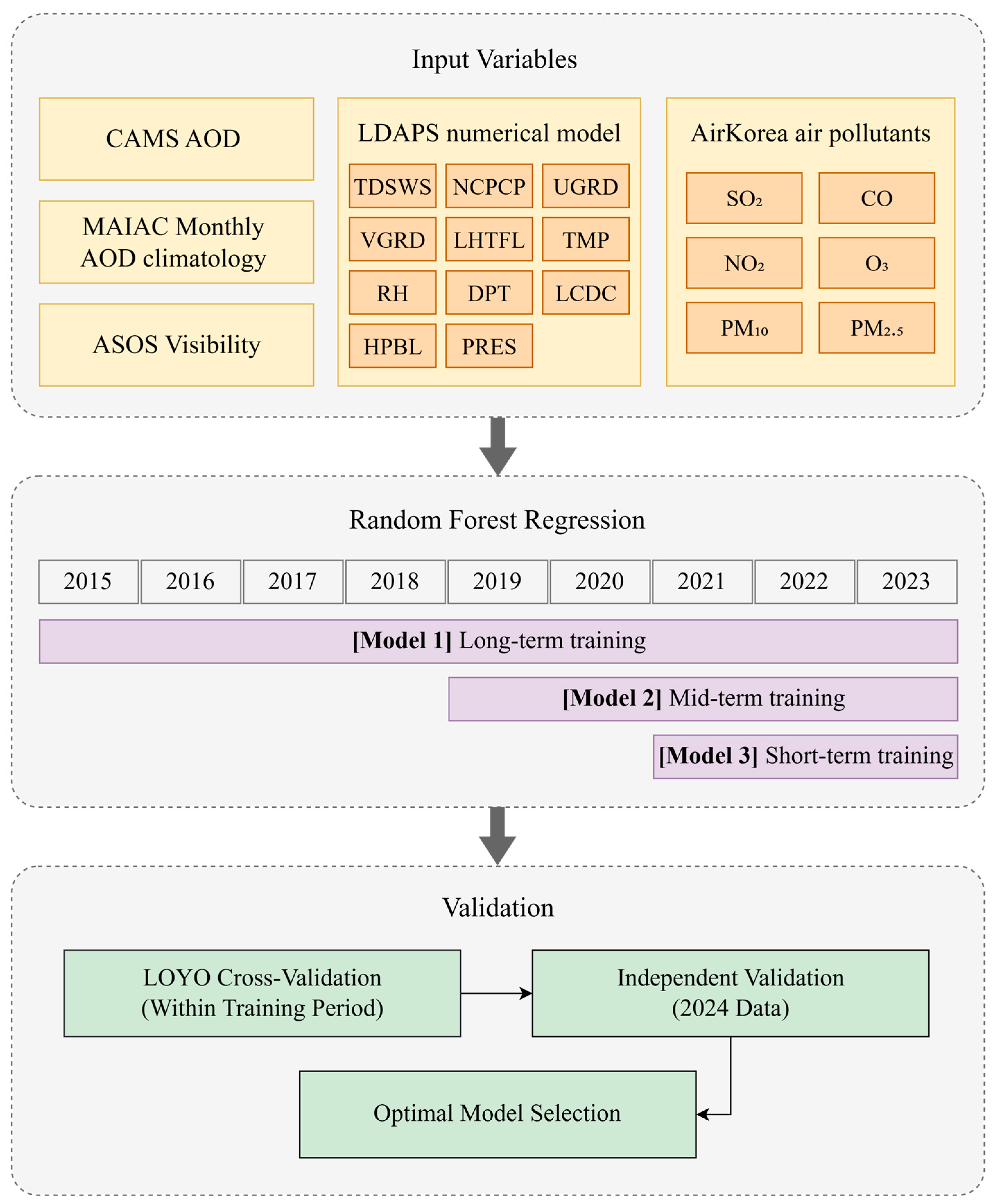
To quantitatively assess the generalization capability and the ability to reflect recent atmospheric composition trends, three RF models were constructed with different training periods (Figure 2): (i) the Full-Period Model (2015–2023), trained on nine years of data to comprehensively capture seasonal and interannual aerosol variability; (ii) the Recent 5-Year Model (2019–2023), emphasizing midterm atmospheric trends and improved sensitivity to recent air quality changes; and (iii) the Recent 3-Year Model (2021–2023), focusing on the most recent aerosol conditions and emphasizing short-term atmospheric states. The three models employed identical input variables, differing only in training duration. The optimal training period was selected based on comparative validation results.

Figure 2. Overview of the Random Forest-based high-resolution AOD retrieval system.

2.5. Real-Time AOD Retrieval Model Evaluation

Model validation was conducted using AERONET Level 2.0 data from 2024, which were not included in training. The 3-hourly AOD outputs at resolution of 1.5 km were compared with AERONET observations matched within a time window of 30 min.

Model performance was evaluated using the metrics such as mean bias, Mean Absolute Error (MAE), RMSE, and correlation coefficient. Additionally, the Expected Error (EE) criterion for land surfaces, defined in the MODIS Collection 6 Dark Target algorithm, ±(0.05 + 0.15 × AERONET AOD), was applied [46]. This threshold accounts for absolute uncertainty (0.05) from surface characteristics, sensor calibration, and aerosol model limitations, as well as relative uncertainty (0.15) proportional to AOD. Retrieval performance is considered acceptable if at least two-thirds (≈66% or ~1 standard deviation) of the estimates fall within this EE envelope [47]. This benchmark has been widely adopted in satellite-based AOD retrieval algorithms, including MODIS, VIIRS, and GOCI [7,48,49].

A multi-level validation strategy was implemented to optimize models trained with different temporal spans. First, Leave-One-Year-Out (LOYO) cross-validation was applied within each training period to evaluate temporal generalization and potential overfitting. Then, the results from the independent 2024 validation set were used to determine the optimal training duration. For the selected optimal model, we conducted the assessment of model performance across land-cover types and the case studies of time-series AOD variations across concentration ranges.

3. Results

3.1. Model Performance

3.1.1. Leave-One-Year-Out Cross-Validation

To evaluate the temporal generalization capability of the three RF models, LOYO cross-validation was performed within each model’s training period (Table 2, Table 3 and Table 4). The long-term training model (2015–2023), Model 1, exhibited consistent performance across all test years, with a mean RMSE of 0.150, a mean MAE of 0.092, and a mean R of 0.825 (Table 2). The mean bias was −0.002, indicating minimal systematic error, and the slight interannual variation in performance suggests that long-term training data contributed to overall model stability.

Table 2. Leave-One-Year-Out (LOYO) cross-validation results for Model 1 with a long-term training period (2015–2023).

Test Year	Bias	MAE	RMSE	R	Samples (Total)
2015	−0.027	0.108	0.175	0.821	2403
2016	−0.028	0.119	0.194	0.798	5346
2017	−0.004	0.098	0.163	0.858	3560
2018	0.035	0.095	0.146	0.855	3384
2019	0.016	0.099	0.158	0.819	2389
2020	0.007	0.075	0.134	0.812	2735
2021	0.009	0.076	0.121	0.827	4016
2022	−0.023	0.078	0.138	0.809	4535
2023	−0.004	0.077	0.125	0.825	5491
Average	−0.002	0.092	0.150	0.825	33,857

Table 3. Leave-One-Year-Out (LOYO) cross-validation results for Model 2 with mid-term training period (2019–2023).

Test Year	Bias	MAE	RMSE	R	Samples (Total)
2019	0.018	0.103	0.166	0.799	2389
2020	0.006	0.075	0.133	0.814	2735
2021	0.013	0.077	0.122	0.823	4016
2022	−0.026	0.078	0.139	0.812	4535
2023	−0.003	0.078	0.126	0.821	5491
Average	0.002	0.082	0.137	0.814	19,166

Table 4. Leave-One-Year-Out (LOYO) cross-validation results for Model 3 with a short-term training period (2021–2023).

Test Year	Bias	MAE	RMSE	R	Samples (Total)
2021	0.025	0.082	0.126	0.820	4016
2022	−0.024	0.079	0.140	0.807	4535
2023	0.003	0.079	0.127	0.818	5491
Average	0.001	0.080	0.131	0.815	14,042

The mid-term model (2019–2023), Model 2, recorded a mean RMSE of 0.137, MAE of 0.082, and R of 0.814 (Table 3). Although the MAE and RMSE were slightly lower than those of Model 1, the R decreased marginally. The model achieved its best performance in 2020–2021 (MAE: 0.075–0.077), with a mean bias close to zero (0.002). The short-term model (2021–2023), Model 3, achieved the lowest overall errors among the three models, with a mean RMSE of 0.131 and MAE of 0.080 (Table 4). The bias was minimal (0.001), and the model maintained stable performance despite the limited training data. However, because LOYO validation was performed only three times, assessment of long-term temporal stability was relatively limited.

Overall, the LOYO results demonstrated that all three models maintained temporal consistency without significant overfitting. The lower errors of the short-term model suggest enhanced responsiveness to recent atmospheric conditions. In contrast, the higher correlation coefficient of the long-term model indicates a superior ability to capture the general spatiotemporal variability of AOD.

3.1.2. Independent Validation with 2024 Data

To evaluate model performance on a fully independent dataset, all three models were validated against AERONET observations from 2024, which were not used in training. Figure 3 presents scatter plots comparing model-predicted AOD with AERONET measurements. All models exhibited similarly high and consistent performance during the independent validation. Model 1 achieved an MAE of 0.075, RMSE of 0.125, and R of 0.841, with 75.8% of predictions falling within the EE range (Figure 3a). Model 2 yielded an MAE of 0.076, RMSE of 0.128, and R of 0.835, with 75.1% within the EE range (Figure 3b). Model 3 showed an MAE of 0.076, RMSE of 0.127, and R of 0.833, with 74.4% within the EE range (Figure 3c). All models exhibited small biases ranging from −0.023 to −0.028, indicating effective control of systematic errors.

Figure 3. Scatter density plots of predicted versus observed AERONET AOD for 2024: (a) Model 1 (trained on 2015–2023), (b) Model 2 (2019–2023), and (c) Model 3 (2021–2023). The black dashed lines represent the 1:1 reference, while red solid lines indicate the linear regression fits. Gray shaded areas denote the MODIS expected error (EE) envelope of ±(0.05 + 0.15 × AOD). The color scale reflects the density of data points.

Particularly, the performance differences observed among the models during LOYO validation nearly disappeared in the independent validation. The differences in MAE and RMSE among the models were within 0.001 and 0.003, respectively, indicating practically equivalent accuracy. Model 1 achieved the highest correlation (R = 0.841) and the most significant fraction within the EE range (75.8%), confirming that the advantages of long-term training persisted even for unseen data. For all models, AOD values were densely concentrated below 0.5, while relatively greater scatter appeared in high AOD regions (AOD > 1.0). Nonetheless, the points were evenly distributed around the 1:1 line, indicating stable predictive performance across a wide range of AOD values.

3.1.3. Optimal Model Selection

Based on a comprehensive evaluation of the LOYO cross-validation and 2024 independent validation results, Model 1 (trained over 2015–2023) was selected as the optimal model (Table 5). Model 1 demonstrated superior performance across multiple metrics. In the 2024 independent validation, it achieved the lowest MAE (0.075) and RMSE (0.125), along with the highest within-EE ratio (75.8%). The model maintained the highest R in both LOYO and independent validation (0.825 and 0.841, respectively), indicating the spatiotemporal variability of AOD. Notably, Model 1 outperformed all other configurations on the fully independent 2024 dataset, confirming its strong predictive capability for future atmospheric conditions.

Table 5. Summary of model performance comparison. Best scores are in bold.

Model	Training Period	LOYO RMSE	LOYO R	2024 RMSE	2024 R
(1) Long-term	2015–2023	0.150	0.825	0.125	0.841
(2) Mid-term	2019–2023	0.137	0.814	0.128	0.835
(3) Short-term	2021–2023	0.131	0.815	0.127	0.833

The performance of Model 1 can be attributed to several advantages provided by nine years of training data. The extended training period encompasses diverse meteorological conditions, seasonal variations in AOD, and extreme pollution episodes, thereby enhancing model robustness. A larger training sample size (33,857 observations) allows the RF ensemble to effectively learn complex nonlinear relationships without overfitting. Furthermore, the long-term dataset captures evolving trends in atmospheric composition and emission patterns, enabling the model to maintain adaptability to recent atmospheric conditions. Therefore, Model 1 was adopted as the final configuration for all subsequent analyses in this study.

The variable importance analysis (Table 6) identifies CAMS AOD as the primary predictor (64%), establishing it as a critical synoptic-scale background for regional estimation. The remaining 36% of the variance is effectively captured by surface air quality and meteorological data. Notably, the high importance of PM2.5 and Visibility (VIS) underscores the model’s ability to incorporate local emission signals and optical properties that coarse-resolution global models often overlook. Furthermore, the significant contributions of DPT, TMP, and LCDC suggest that the model correctly reflects the physical processes of hygroscopic growth and aerosol-cloud interactions.

Table 6. Feature importance of the optimal model.

Feature	Importance	Feature	Importance
CAMS	0.63665	VGRD	0.01598
PM25	0.04931	TDSWS	0.01588
VIS	0.04479	PRES	0.01584
DPT	0.02530	HPBL	0.01562
TMP	0.02491	NO2	0.01479
LCDC	0.02463	RH	0.01450
PM10	0.01995	LHTFL	0.01344
O3	0.01692	SO2	0.00782
UGRD	0.01675	CO	0.00726
Monthly Climatology	0.01655	NCPCP	0.00310

3.2. Performance by AERONET Site and Land Cover Type

Because the CAMS AOD forecast fields are generated by numerical modeling with satellite data assimilation, they reflect characteristics of satellite-based AOD retrievals. Satellite AOD is typically derived by inverting TOA reflectance, which is more sensitive to aerosol signals over dark surfaces than over bright surfaces [50]. To assess the impact of surface reflectance on AOD retrieval uncertainty, we evaluated model performance by land cover types. Land cover was classified using the MODIS land cover product (MCD12Q1) into categories (e.g., urban, forest, cropland, and coastal). The dominant land-cover category within a 10 km × 10 km window centered on each station was then assigned to that site.

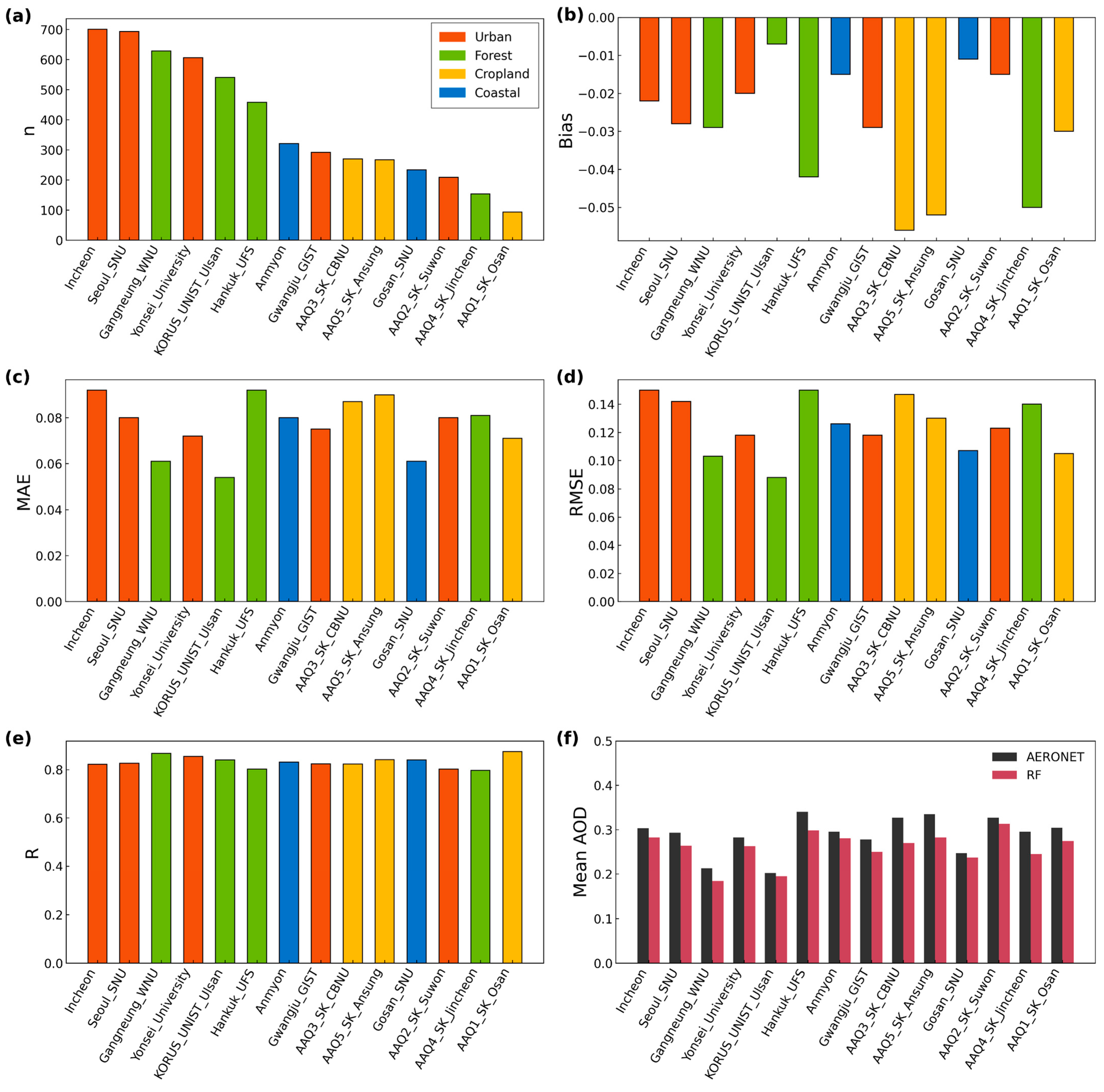
Figure 4 summarizes validation statistics and mean AOD distributions for 14 AERONET sites. Most sites exhibited strong performance, with MAE and RMSE generally in the ranges 0.06–0.09 and 0.10–0.15, respectively. Among individual sites, Gangneung_WNU in forest areas showed the best results, to which low mean AOD and stable atmospheric conditions likely contributed (Figure 4f). In contrast, Hankuk_UFS and sites in cropland areas, often adjacent to urban districts and influenced by mixed emission sources, displayed relatively larger errors (Figure 4c,d). Major urban stations (Seoul_SNU, Yonsei_University, and Incheon) maintained consistent performance despite the complexity of urban environments (Figure 4e). Overall, the model achieved correlations exceeding 0.80 at most sites with minimal systematic bias (Figure 4b).

Figure 4. (a–e) Bar charts showing sample size (n), bias, MAE, RMSE, and correlation coefficient (R) by AERONET site, color-coded by land cover: Urban (orange), Forest (green), Cropland (yellow), and Coastal (blue). (f) Mean AOD comparison between AERONET (black) and RF model (red) across all sites.

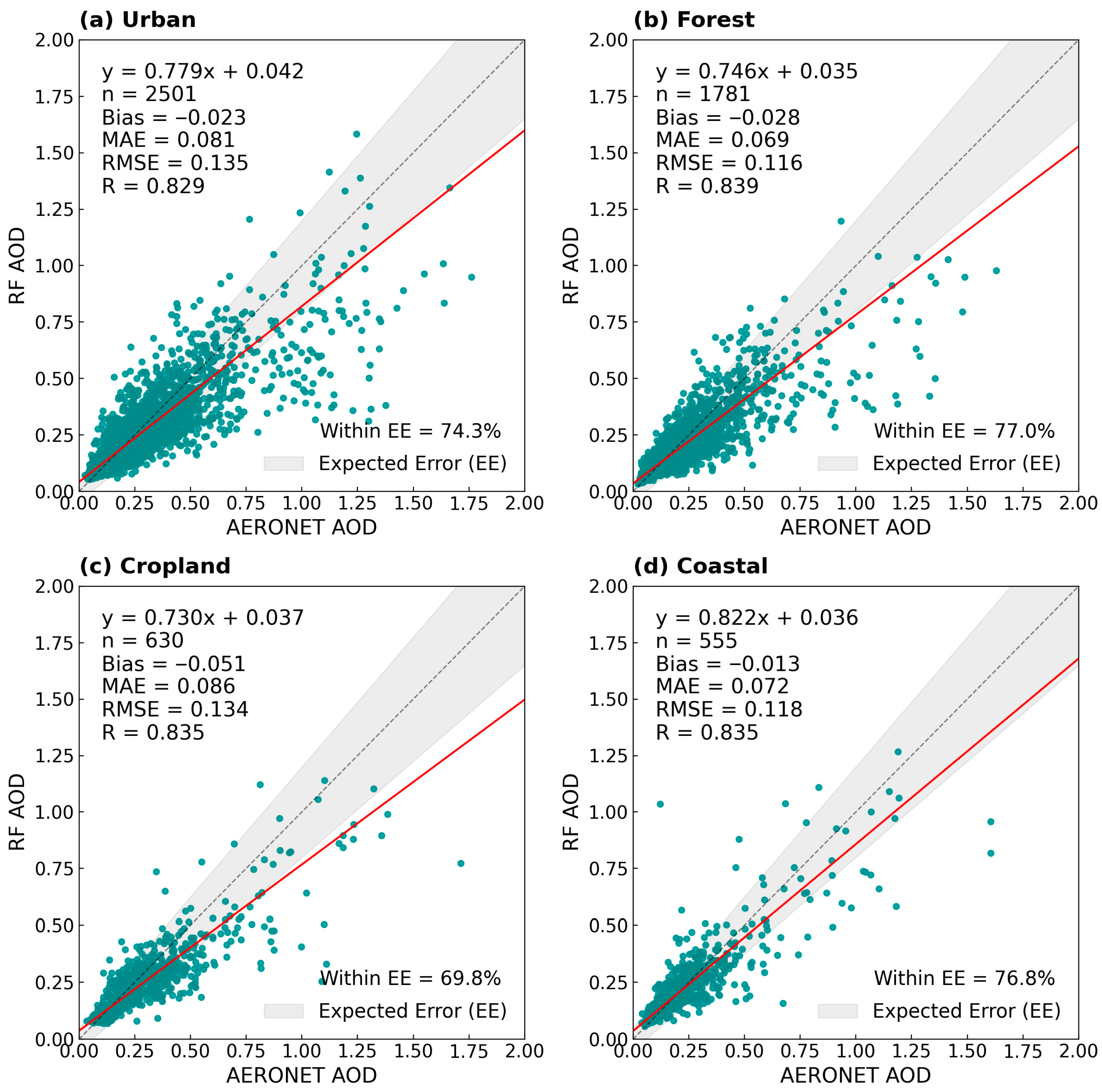
The results for each station by land cover type are presented in Figure 5. The model performed robustly across all surface conditions. In particular, Forest sites achieved the lowest MAE (0.069) and RMSE (0.116), representing the best performance among the four land-cover classes (Figure 5b). A correlation of 0.839 and a slight bias (−0.028) suggest that the relatively dark forest background facilitates effective capture of aerosol signals in the satellite-informed CAMS forecasts.

Figure 5. Scatter density plots of RF-predicted versus AERONET-observed AOD for 2024, categorized by land cover type: (a) Urban, (b) Forest, (c) Cropland, and (d) Coastal. The black dashed lines represent the 1:1 reference, the red solid lines indicate the linear regression fits, and the gray shaded areas denote the MODIS expected error (EE) envelope of ±(0.05 + 0.15 × AOD).

Coastal regions also showed strong performance (MAE = 0.072; RMSE = 0.118; R = 0.835), with balanced predictions across the full AOD range and the smallest bias (−0.013) among all classes, indicating stable model behavior in marine-influenced environments (Figure 5d).

The urban class, validated with the most significant sample (n = 2501), yielded an MAE of 0.081, RMSE of 0.135, and R of 0.829, demonstrating good performance and high correlation despite complex emission mixtures, suggesting that the model adequately represents diverse urban aerosol sources (Figure 5a).

Cropland regions exhibited an MAE of 0.086, RMSE of 0.134, and R of 0.835 along with a relatively larger bias (−0.051) compared with other classes (Figure 5c). This is likely due to the coexistence of urban and industrial activities near agricultural zones, where heterogeneous aerosol types increase retrieval uncertainty.

Across all land-cover types, correlation coefficients exceeded 0.83, confirming that our model delivers robust AOD estimation performance regardless of surface characteristics.

3.3. Performance by Season

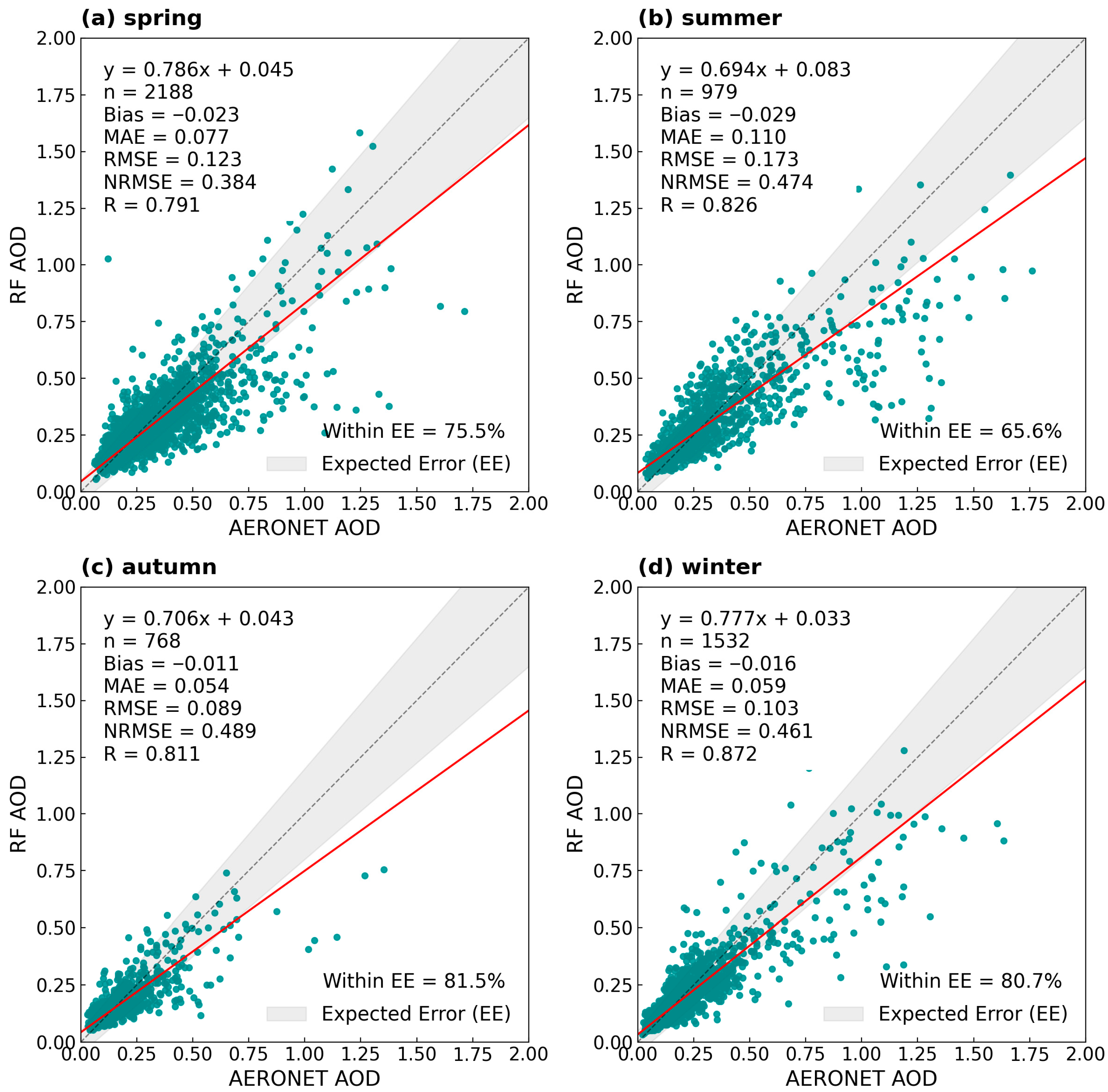
The performance validation across all four seasons demonstrated that the proposed model yields consistently high accuracy in estimating AOD over South Korea. As shown in the seasonal scatter plots (Figure 6), the RF-derived AOD values generally align well with the reference AERONET observations, with the majority of data points falling within the EE envelope. Quantitatively, the correlation with the AERONET remained strong and stable, ranging from a minimum of R = 0.791 in spring to a maximum of R = 0.872 in winter. Furthermore, the model exhibited a low systematic offset, with the bias staying very close to zero across all seasons (e.g., –0.023 in spring and –0.011 in autumn). The MAE and RMSE metrics confirmed the robustness of the model performance. We observed notably low error ranges: MAE fluctuated between 0.054 (autumn) and 0.110 (summer), and RMSE varied between 0.089 (autumn) and 0.173 (summer). Recognizing the slight seasonal variability inherent in these absolute error metrics, we calculated the Normalized Root Mean Square Error (NRMSE), utilizing the seasonal mean AOD as the normalization factor, to better assess the inherent spread relative to the mean. The calculated NRMSE values demonstrated high stability across all seasons, spanning a narrow range from 0.384 to 0.489. The consistency shown by NRMSE, despite the seasonal changes in absolute RMSE, strongly suggests that the model is well-calibrated and reliably meets the stringent quality requirements for satellite AOD products consistently throughout the year.

Figure 6. Seasonal scatter density plots of RF-predicted versus AERONET-observed AOD in 2024: (a) Spring, (b) Summer, (c) Autumn, and (d) Winter. The black dashed lines represent the 1:1 reference, the red solid lines indicate the linear regression fits, and the gray shaded areas denote the expected error (EE) envelope of ±(0.05 + 0.15 × AOD).

3.4. Time-Series Analyses for Various AOD Events

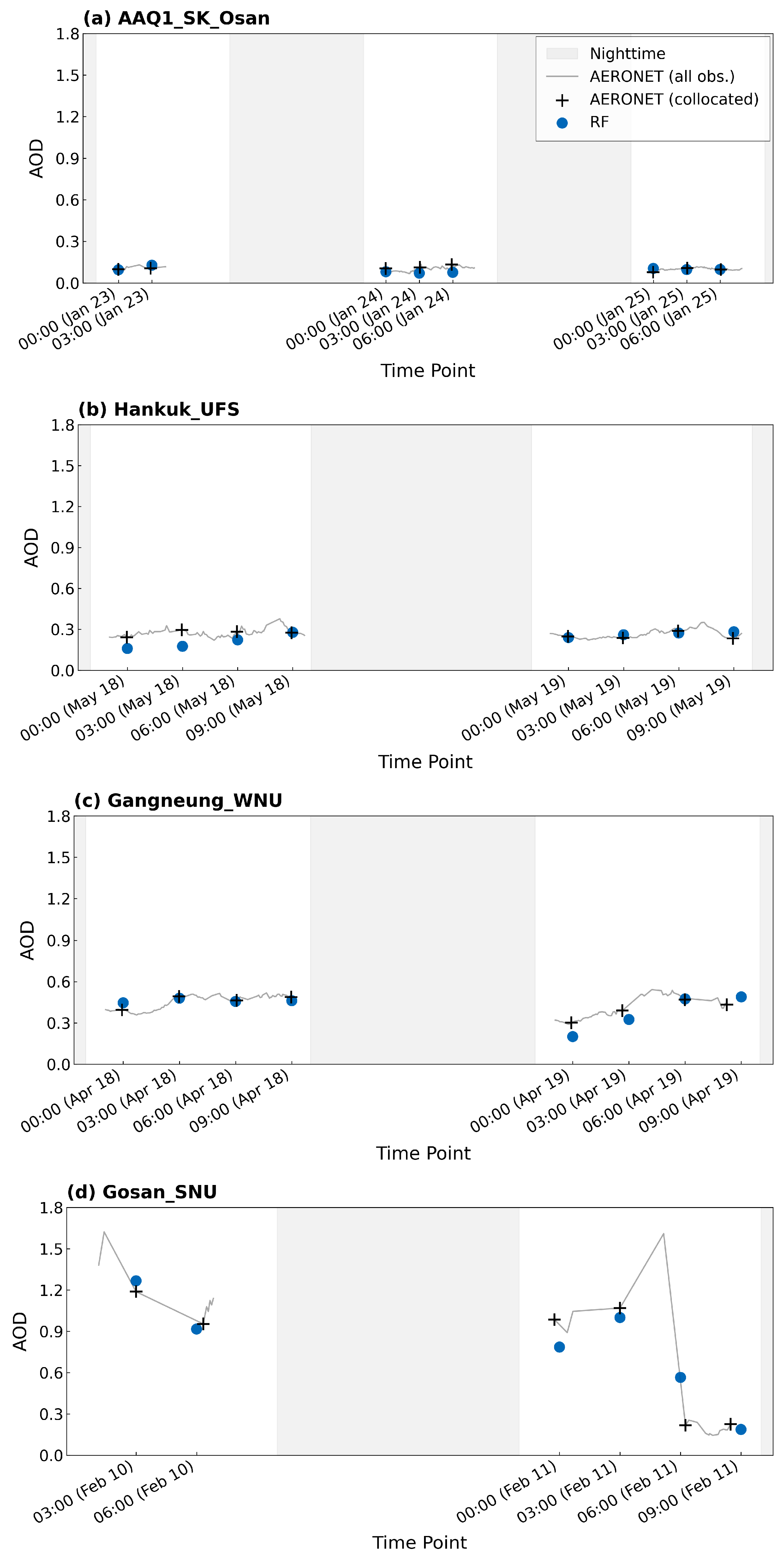
To evaluate changes in model performance under different pollution levels, AERONET AOD observations were categorized into four concentration ranges for 2024: clean atmosphere (0.0–0.2), thin aerosols (0.2–0.4), thick aerosols (0.4–0.8), and very thick aerosols (≥0.8). Figure 7 presents representative time-series comparisons of RF-model AOD and AERONET observations for each class.

Figure 7. Time series comparison of RF model AOD (blue dots) and AERONET AOD observations (black crosses with gray line) for representative cases across different AOD ranges: (a) Clean (0.0–0.2, AAQ1_SK_Osan), (b) Thin (0.2–0.4, Hankuk_UFS), (c) Thick (0.4–0.8, Gangneung_WNU), and (d) Very Thick (≥0.8, Gosan_SNU). Shaded gray areas mark nighttime, when AERONET data are unavailable.

Under clean-air conditions (Figure 7a), observations from the AAQ1_SK_Osan site during January 23–25 indicate a low-concentration episode. This period represents a typical winter meteorological pattern characterized by cold-air mass intrusions and clean atmospheric conditions. The RF model closely tracked AERONET, reproducing AOD below 0.1 and accurately following the observations on 23 and 25 January. This indicates stable performance even under low signal-to-noise conditions, enabled by effective fusion of diverse predictors. RF estimates were not generated during nighttime (shaded areas) when AERONET observations are unavailable.

For the thin aerosol range (Figure 7b), the Hankuk_UFS case from 18–19 May is shown. The RF model captured the diurnal pattern in the 0.2–0.3 range but underestimated by approximately 0.1 at 00 UTC on 18 May. This transient error likely reflects the combined effects of a shallow morning boundary layer and the interplay among input variables. The agreement improved markedly after 03 UTC as the boundary layer developed, consistent with the stabilization of daytime conditions. On 19 May, the model maintained consistent accuracy across all hours, and 3-hourly predictions aligned well with the continuous AERONET trend, suggesting rapid adaptation to transient meteorological variability.

For thick aerosol conditions (Figure 7c), a high-loading episode at Gangneung_WNU is shown, characteristic of springtime pollution with AOD rising to 0.4–0.5. Our model closely tracked AERONET on both days, reproducing persistently high AOD on 18 April and the increasing trend on 19 April. Minor deviations from observations at specific time points, but overall temporal variability was well captured, demonstrating robust performance under elevated aerosol burdens.

For very thick aerosols (Figure 7d), we examine an extreme transboundary event that occurred at Gosan_SNU (February 10–11). On February 10, during the Chinese Lunar New Year, intensive fireworks and industrial emissions were likely transported eastward by the westerlies, resulting in a canonical long-range transport case. Extreme AOD (>1.2) was observed at 03 UTC on 10 February, followed by a gradual decrease as the polluted air mass shifted eastward and atmospheric dispersion increased. the proposed model reproduced both the rapid concentration changes and the subsequent decline. Some discrepancies likely reflect greater uncertainty in the predictors under extreme conditions. Overall, the model captured the transition from very high loading to cleaner conditions, indicating utility for monitoring the temporal evolution of severe dust and transboundary pollution events.

In summary, the proposed model successfully reproduced the 3-hourly AOD variability across the full spectrum of atmospheric loading, from clean to highly polluted conditions. Its performance was remarkably stable under low-to-moderate conditions (AOD < 0.8), accurately capturing both diurnal and day-to-day variability, and also faithfully reflecting the temporal evolution of extreme events. This high versatility across diverse atmospheric regimes supports the practical applicability of the system for real-time AOD monitoring.

3.5. Creation of High-Resolution Gap-Free AOD Maps

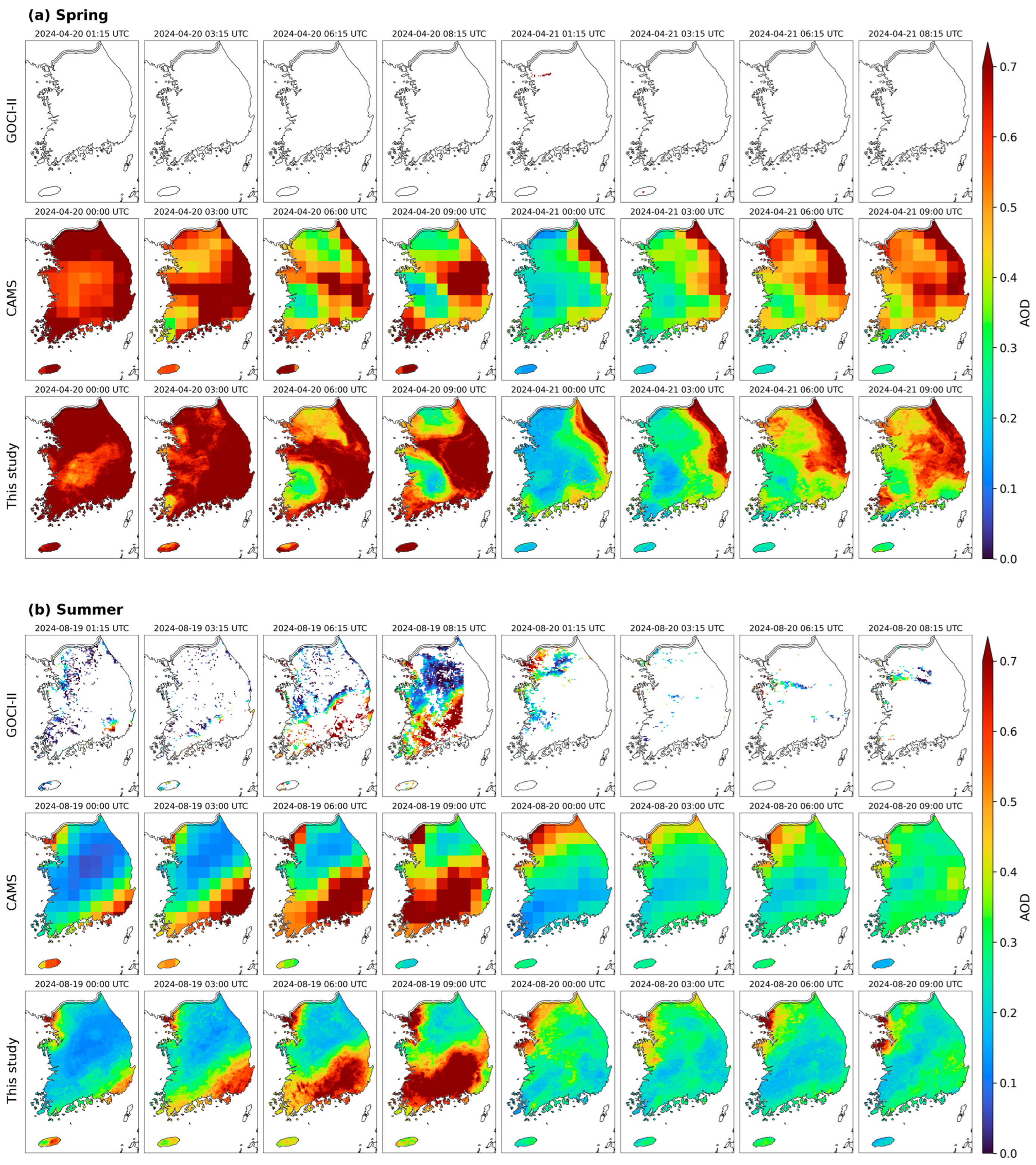
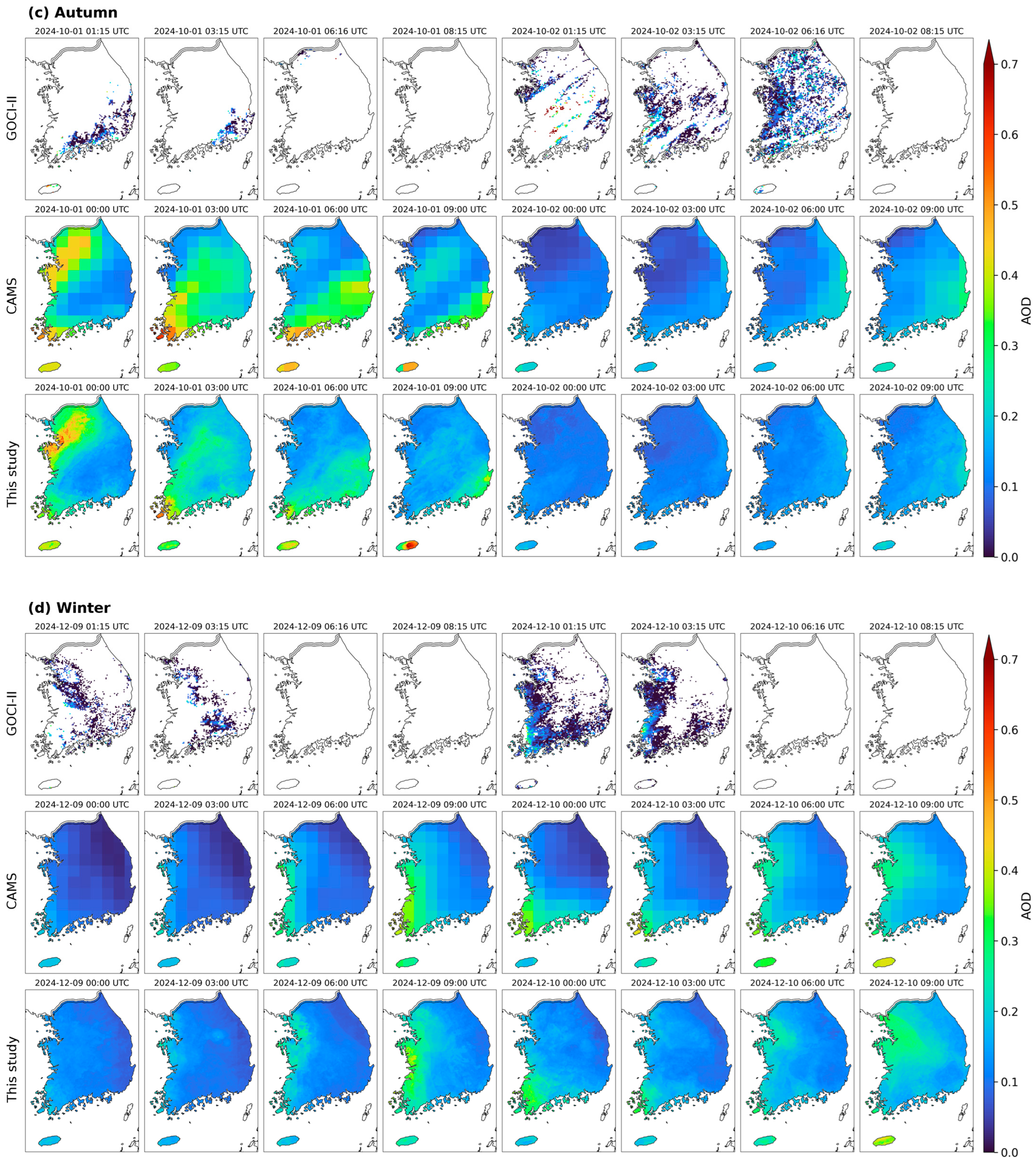
To evaluate seasonal spatial patterns and demonstrate the gap-filling capability of the proposed model, we compared two consecutive days from each season in 2024 against CAMS forecasts and satellite observations (Figure 8). Specifically, we utilized retrievals from the Geostationary Ocean Color Imager II (GOCI-II), South Korea’s geostationary satellite, to facilitate continuous comparisons between our gap-free products and operational satellite datasets. The selected periods were Spring (April 20–21), Summer (August 19–20), Autumn (October 1–2), and Winter (December 9–10). Three AOD products were evaluated at 3-hourly intervals: satellite-derived GOCI-II retrievals (~3 km resolution, matched to the nearest hours at 00, 03, 06, and 09 UTC), CAMS forecasts (~40 km resolution), and our RF model retrievals (1.5 km resolution).

Figure 8. Seasonal comparison of AOD products over South Korea in 2024. Each panel displays two consecutive days for each season: (a) Spring (April 20–21), (b) Summer (August 19–20), (c) Autumn (October 1–2), and (d) Winter (December 9–10). The rows represent GOCI-II retrievals (top; 3 km resolution), CAMS forecasts (middle; ~40 km resolution), and the proposed RF model (bottom; 1.5 km resolution). All data are presented at 3-hourly intervals from 00:00 to 09:00 UTC, with GOCI-II matched to the nearest available observation times.

The GOCI-II AOD exhibited pervasive spatial gaps due to cloud contamination (Figure 8a,b) and limited retrievals during winter caused by shortened daylight hours (Figure 8d). Such extensive data loss fundamentally constrains the utility of satellite products for operational air quality monitoring, where continuous coverage is essential. While CAMS forecasts are gap-free, their coarse resolution fails to resolve local-scale variability, often smoothing aerosol distributions into broad regional patterns. In contrast, our RF model provided seamless, gap-free coverage while capturing fine-scale spatial gradients across all seasons.

In Spring (Figure 8a), when dust intrusions and local emissions drove high AOD (>0.4) along the western coast, GOCI-II failed to provide any retrievals due to extensive cloud cover. This highlights the inherent limitations of optical satellite observations. Our model, however, clearly delineated the spatial extent and eastward progression of these elevated AOD zones, identifying localized hotspots that CAMS represented as diffuse patterns. Summer (Figure 8b) similarly showed fragmented GOCI-II coverage, whereas the developed model captured fine-scale gradients over metropolitan areas. In Autumn (Figure 8c) and Winter (Figure 8d), the RF model maintained continuous spatial distributions even under shortened daylight conditions and low aerosol loading (AOD < 0.2), resolving subtle coastal variations.

Overall, the proposed RF model effectively addresses the complementary weaknesses of existing systems: the cloud-induced gaps in satellite retrievals and the inadequate spatial resolution of global forecast models. This advancement enables high-resolution, continuous monitoring of aerosol variability, a capability vital for operational air quality surveillance over the Korean Peninsula.

4. Discussion

4.1. Comparison with CAMS Baseline

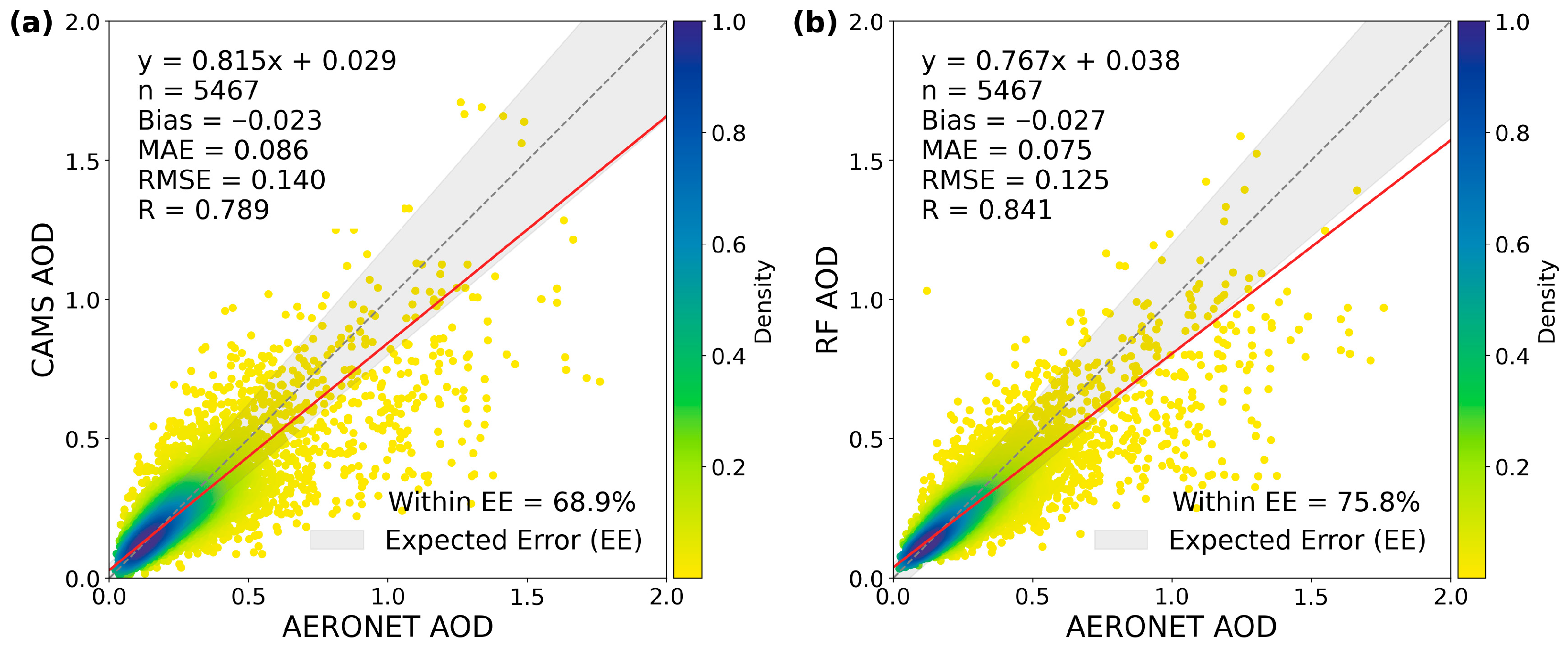
We developed a real-time, high-resolution, 3-hourly AOD retrieval system based on AERONET observations, using CAMS AOD forecasts as a key input variable and adding satellite AOD climatology from MODIS, meteorological variables from LDAPS, and air quality observations from AirKorea. Although CAMS provides global-scale AOD forecasts, its coarse spatial resolution (approximately 40 km) limits regionally accurate monitoring. Figure 9 compares the original CAMS predictions and our model’s outputs with AERONET observations as ground truth for the entire year of 2024.

Figure 9. Scatter density plots comparing AOD retrievals with AERONET observations for the full year of 2024: (a) original CAMS forecast and (b) the proposed RF model. The black dashed lines represent the 1:1 reference, the red solid lines indicate the linear regression fits, and the gray shaded areas denote the expected error (EE) envelope. The color bars represent the density of data points.

The original CAMS forecasts (Figure 9a) achieved MAE 0.086, RMSE 0.140, and R 0.789, capturing the general variability of AOD but failing to reproduce detailed local fluctuations, as reflected by the lower correlation. In contrast, the proposed model (Figure 9b) yielded MAE 0.075, RMSE 0.125, and R 0.841, demonstrating substantial improvements across all statistical metrics. The correlation increased from 0.789 to 0.841, indicating a better representation of local-scale AOD variability. While CAMS exhibits a favorable slope (0.815)—reflecting a physics-based framework that preserves the dynamic range—it suffers from higher variance. In contrast, our RF model substantially reduces scatter through statistical optimization, effectively minimizing both systematic biases and random errors to enhance operational performance.

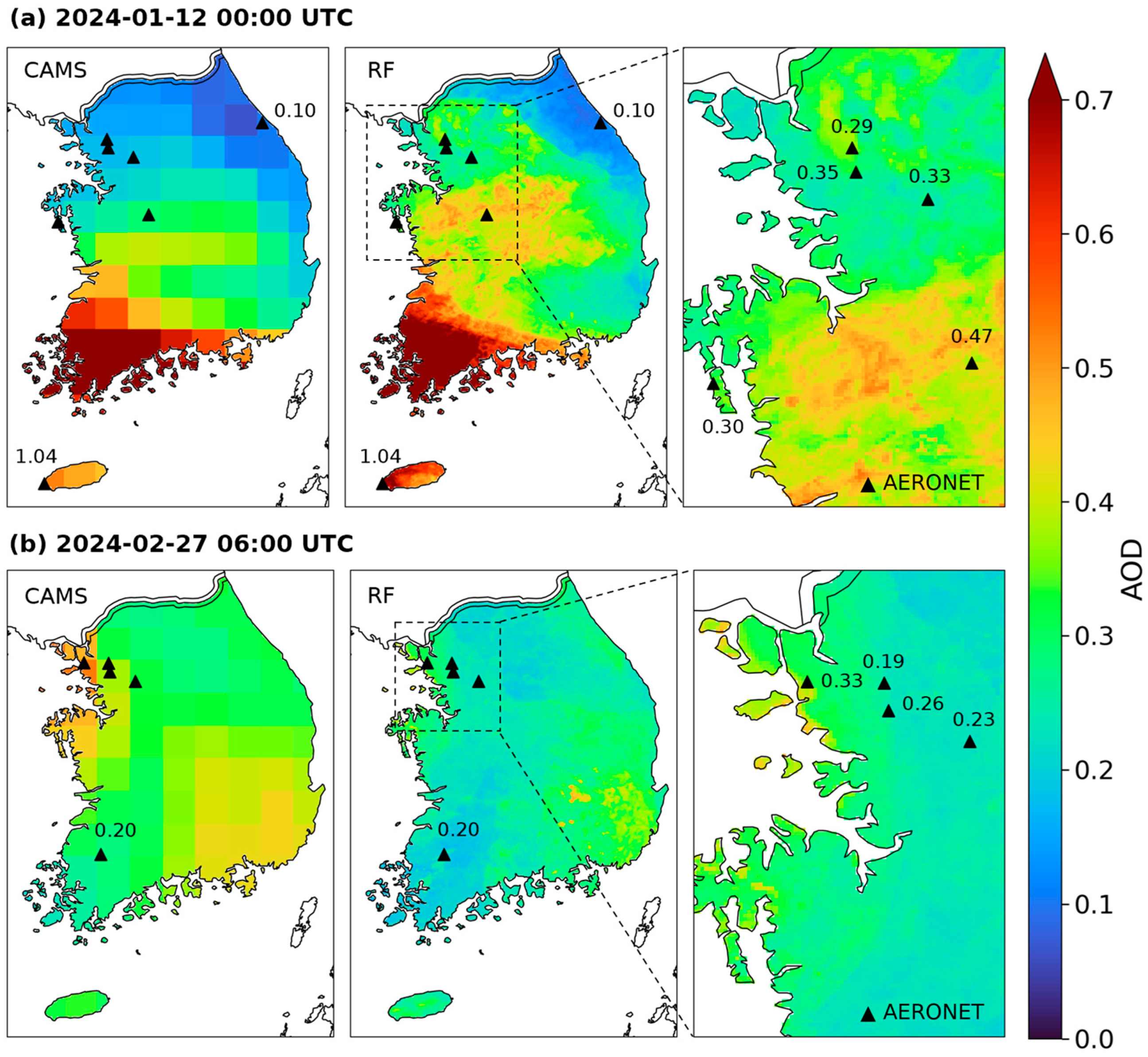
Table 7 and Figure 10 present representative examples illustrating the differences in spatial reproduction capability between the CAMS forecasts and the RF-derived AOD fields. Figure 10a shows a high aerosol loading episode on 12 January 2024, with the Gosan_SNU AERONET site recording an AOD of 1.04. CAMS underestimated AOD at most observation sites due to its coarse spatial resolution, representing the high concentration belt across the west coast and southern regions only as broad regional averages. In contrast, the proposed model successfully captured the fine-scale spatial structure of elevated AOD extending from the southwestern coast to the central inland areas. The magnified panel shows that our model resolves localized variations over the Seoul Metropolitan Area and the west coast (AOD 0.2–0.47) at fine scales.

Table 7. Comparison of CAMS and our model AOD regarding multiple AERONET sites.

Date and Time	Station	Latitude (°)	Longitude (°)	CAMS	Ours	AERONET
2024011200	Gosan_SNU	33.29222	126.1617	0.524	0.725	1.044
2024011200	Anmyon	36.53854	126.3302	0.199	0.321	0.301
2024011200	AAQ3_SK_CBNU	36.62630	127.4566	0.290	0.387	0.472
2024011200	Hankuk_UFS	37.33883	127.2658	0.183	0.259	0.334
2024011200	Seoul_SNU	37.45806	126.9511	0.174	0.300	0.348
2024011200	Yonsei_University	37.56443	126.9348	0.174	0.364	0.298
2024011200	Gangneung_WNU	37.77100	128.8670	0.104	0.124	0.097
2024022706	Gwangju_GIST	35.22828	126.8431	0.280	0.197	0.200
2024022706	Hankuk_UFS	37.33883	127.2658	0.320	0.227	0.226
2024022706	Seoul_SNU	37.45806	126.9511	0.380	0.258	0.262
2024022706	Yonsei_University	37.56443	126.9348	0.380	0.263	0.191
2024022706	Incheon	37.56882	126.6372	0.529	0.328	0.330

Figure 10. Comparison of CAMS and our model AOD spatial distributions for (a) high AOD case (January 12) and (b) moderate background case (February 27). Triangles indicate AERONET station locations with observed AOD values. The right panels show magnified views of the metropolitan region with detailed AERONET station values.

Figure 10b depicts a moderate background case on 27 February 2024, when most AERONET observations ranged from 0.19 to 0.33. CAMS produced a spatially extensive, moderately high AOD field across the western region, including the Seoul metropolitan area. This failed to capture the observed clean state. In contrast, the proposed model accurately reproduced the nationwide background AOD levels (0.2–0.3). The zoomed-in map shows detailed spatial differentiation over the areas surrounding Seoul (0.1–0.33).

In both cases, the RF model restored fine-scale AOD variability smoothed in the CAMS forecasts. The retrieved fields closely matched AERONET observations. The model corrected both CAMS underestimation during high AOD episodes and overestimation under clean conditions, producing distributions more consistent with ground truth. These results confirm that our model goes beyond simple spatial interpolation of CAMS fields, instead using additional predictors, such as meteorological and air pollutant variables, to reproduce AERONET-observed AOD distributions more accurately.

The proposed model outperformed the original CAMS forecasts across all evaluation metrics, achieving genuine accuracy improvements beyond those achievable through interpolation alone. By integrating satellite AOD climatology, meteorological variables, and air quality observation, the model effectively transformed sparse AERONET point observations into a spatially continuous field. As is also evident from the seasonal comparisons in Figure 8, the proposed method successfully captured urban-scale aerosol distributions and localized variability that global CAMS forecasts could not resolve. These results demonstrate that the proposed system provides an AOD product that is operationally applicable for air quality monitoring and forecasting.

CAMS is known to underestimate AOD in East Asia, with a Modified Normalized Mean Bias (MNMB) of −15% to −25% [51]. Since CAMS AOD is our most dominant predictor (importance = 0.64), the model inevitably inherits some of this signal. However, the two-step multi-resolution approach does not introduce systematic underestimation.

• Bias Reduction, not Inheritance: Our model actually reduces the bias magnitude compared to the raw CAMS data. For instance, while CAMS often shows biases exceeding 20%, our model maintains an MBE of around −0.02, demonstrating that the integration of high-resolution LDAPS and AirKorea data effectively performs bias correction rather than just inheriting error.
• Scale Invariance of Meteorological Relationships: Regarding the aggregation of predictors, we aggregated 1.5 km LDAPS data to 40 km during Step-1 to ensure a consistent spatial scale with CAMS. While the absolute values of variables (e.g., humidity, wind speed) may differ slightly between 1.5 km and 40 km, the physical relationship between these meteorological variables and AOD remains relatively stable across these scales. Therefore, the learned bias-correction rules remain valid when high-resolution inputs are applied in Step-2.
• Effective Downscaling: Our approach treats the 40 km CAMS data as a coarse prior and uses high-resolution meteorological and surface features to refine the spatial gradients. As seen in Figure 8, our model captures fine-scale urban/industrial plumes that are absent in the coarse CAMS fields, which would not be possible if the aggregation had suppressed the model’s learning capacity.

4.2. EOF Analysis for Spatiotemporal Variability

The developed AOD product exhibited a strong correlation with AERONET observations (R = 0.841); however, ground-based validation alone cannot fully characterize the spatiotemporal variability of the entire domain. Over Korea, AOD is governed by complex interactions among local emissions, meteorological conditions, and transboundary transport from China. Therefore, an additional evaluation was conducted to verify whether the retrieved product appropriately reproduces these physical patterns. To this end, an EOF analysis was applied to the daily mean AOD field for 2024, decomposing the spatiotemporal dataset into principal spatial modes (EOFs) and their corresponding temporal coefficients (principal components, PCs). Each EOF mode characterizes large-scale mechanisms that are difficult to identify from point observations, while the associated PC quantifies the temporal evolution of each spatial pattern.

The analysis was performed using AOD anomalies over South Korea, focusing on variability rather than absolute magnitudes. PCs were standardized using Z-scores, so that positive (PC > 0) and negative (PC < 0) values represent deviations above or below the mean variability, respectively.

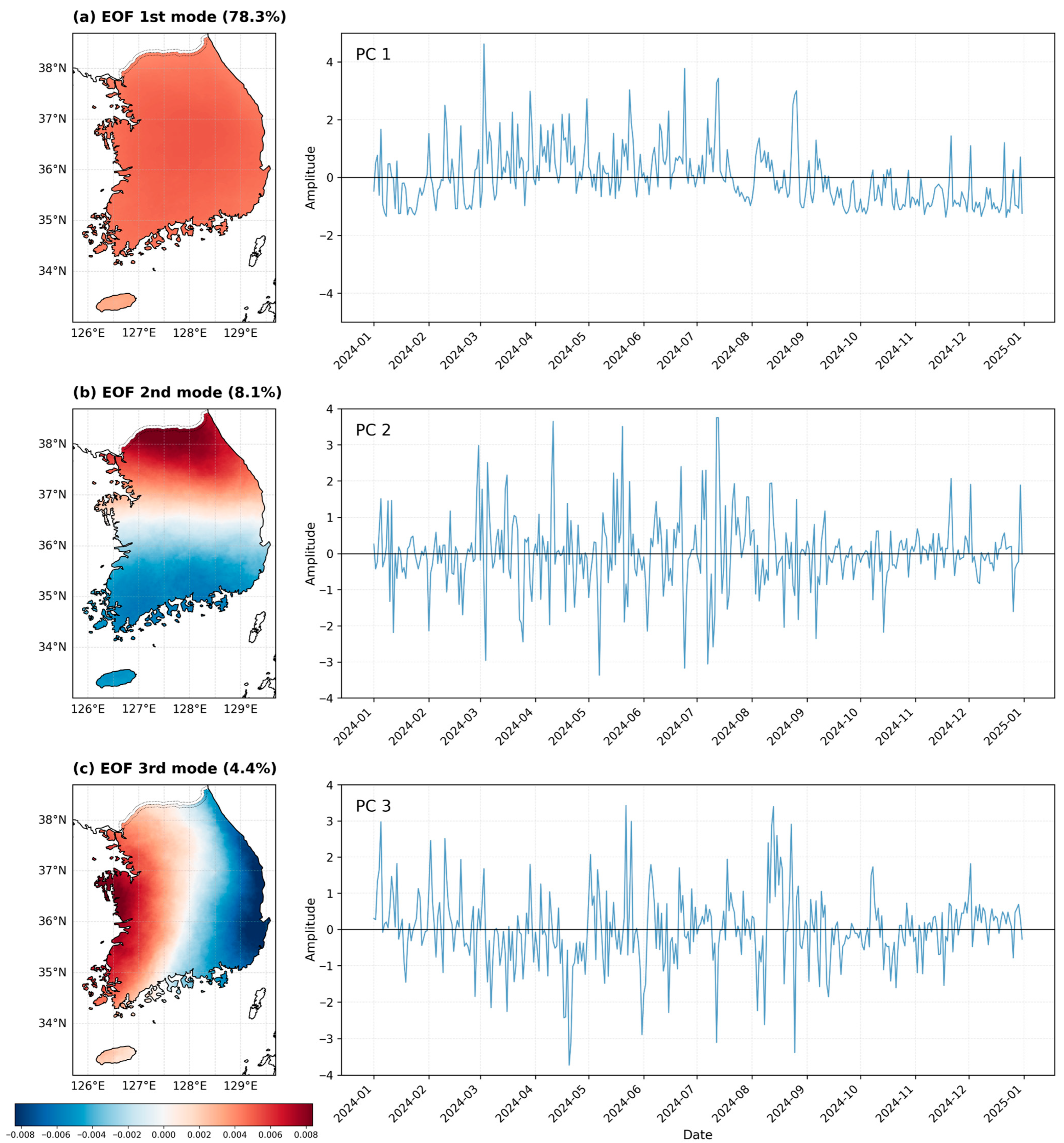
The EOF analysis of daily mean AOD for 2024 revealed three dominant modes, which together explained 90.8% of the total variance. The first mode (EOF1) accounted for approximately 78.3% of the total variance (Figure 11a). Spatially, it exhibited nearly uniform positive loadings (PC1 > 0) across the Korean Peninsula, indicating that AOD variability is primarily controlled by synoptic-scale atmospheric circulation rather than local emission sources. This coherent pattern of nationwide increases or decreases reflects the dominant influence of continental-scale factors such as long-range transport, synoptic pressure patterns, and ventilation efficiency. The PC1 time series displayed a clear seasonal cycle: positive values during spring and summer (March–August) correspond to high AOD episodes driven by continental aerosol influx under northwesterly flow and enhanced photochemical activity [52,53,54], whereas sustained negative values during autumn and winter (September–February) reflect cleaner conditions associated with weakened transport and stronger atmospheric stability.

Figure 11. Empirical orthogonal function (EOF) decomposition of the Korea-domain AOD field for 2024. The left panels show spatial loadings (unitless), and the right panels show the corresponding standardized principal component (PC) time series. The fraction of explained variance by each mode is indicated in parentheses: (a) Mode 1 (78.3%), (b) Mode 2 (8.1%), and (c) Mode 3 (4.4%). The sign of the patterns is arbitrary; positive PC values indicate an increase in AOD over red areas and a decrease over blue regions.

The second mode (8.1% of variance, Figure 11b) displays a north–south dipole pattern, with positive loadings over the Seoul Metropolitan Area and negative loadings along the southern coast. The PC2 time series showed weaker seasonality and higher-frequency fluctuations than PC1, suggesting transient synoptic variability and episodic local emissions. Positive phases (PC2 > 0) represent increased AOD in northern Korea, typically associated with continental inflow under northwesterly winds. Polluted air masses transported from north and eastern China first reach northwestern Korea (e.g., Seoul, Incheon, and the Chungnam coastal region), where they interact with strong local emissions, enhancing AOD through secondary aerosol formation [55]. As these air masses move southeastward, dispersion leads to lower AOD over the southern regions. Conversely, negative phases indicate enhanced AOD in the south, likely linked to southerly flows, moisture advection, or local stagnation events.

The third mode (EOF3), explaining 4.4% of the total variance (Figure 11c), showed an east–west contrast, with positive loadings along the west coast and negative loadings over the east. The positive phase corresponds to AOD enhancement along the western coast and major urban areas under westerly winds. In contrast, the negative phase reflects higher AOD in eastern or mountainous inland regions. This pattern arises under easterly or northeasterly flow, when the Taebaek Mountains block ventilation and induce stagnation on the east side. Under such conditions, industrial emissions in Ulsan, Pohang, and Busan accumulate due to limited dispersion, and frequent springtime wildfires in the eastern mountains can further elevate AOD levels [56]. In contrast, subsiding air on the western slopes promotes ventilation, maintaining relatively lower AOD there.

Collectively, the three EOF modes demonstrate that the developed AOD product successfully reproduces (i) the dominant national-scale seasonal and synoptic signals (EOF1) and (ii) physically interpretable regional gradients (EOF2–EOF3) that are often obscured in coarse-resolution datasets. In particular, the east–west contrast in EOF3 provides statistical evidence for episodic increases in AOD over eastern Korea relative to the west.

By providing spatiotemporally continuous data, the product captures aerosol dynamics across multiple scales, from continental long-range transport to topography and meteorology-driven local variability, thus going beyond site-level replication to faithfully reproduce the spatiotemporal mechanisms of aerosol variability over the Korean Peninsula. Importantly, whereas such regional patterns (e.g., the north–south dipole in EOF2 and east–west contrast in EOF3) were indistinct in the coarse CAMS fields, they were clearly resolved in our high-resolution AOD product.

5. Conclusions

We developed a real-time AOD retrieval system over South Korea, which provides high-resolution, gap-free, 3-hourly data by integrating CAMS forecasts, MODIS AOD climatology, LDAPS meteorological fields, and ground-based air-quality observations within an RF framework. Unlike traditional cloud-prone satellite retrievals and latency-afflicted, coarse reanalysis data, our AI model produces AOD products that are real-time, high-resolution, and spatially continuous. Moreover, the proposed model provides superior accuracy compared to the original CAMS data and shows stable performance irrespective of land cover types and seasons.

Utilizing CAMS forecasts eliminates production latency, enabling 3-hourly operational AOD retrievals. The integration of high-resolution LDAPS meteorology and AirKorea air-quality data allows the model to incorporate key physical processes like hygroscopic growth, secondary aerosol formation, and transport dynamics. This achieves physically consistent downscaling, moving beyond simple statistical interpolation. Our model outputs represent Korea’s complex terrain and heterogeneous emission sources in detail, producing spatiotemporally continuous data that effectively mitigate cloud-related gaps in satellite observations. Long-term training over nine years further enhanced model robustness across diverse meteorological conditions and aerosol concentration ranges.

Independent validation for 2024 (trained on 2015–2023 data) confirmed strong performance, yielding a MAE of 0.075, RMSE of 0.125, R of 0.841, and achieving 75.8% of predictions within the MODIS expected error range. These metrics represent marked improvement over the original CAMS forecasts and show comparable accuracy to established satellite AOD retrieval algorithms. Consistent and robust performance was observed across all land-cover types (urban, forest, cropland, and coastal) and AOD ranges (0.0–1.0+).

EOF analysis further revealed that the AOD product successfully captured Korea’s dominant aerosol patterns: (1) Nationwide seasonal variability driven by long-range transport (EOF1, 78.3%), (2) North–south gradients between the Seoul Metropolitan Area and southern regions (EOF2, 8.1%), and (3) East–west contrasts induced by the Taebaek Mountains (EOF3, 4.4%). This confirms that the proposed system physically and statistically captures aerosol dynamics from continental to local scales, moving beyond simple point-based emulation.

The system’s future applications include real-time air-quality surveillance, pollution source tracking, aerosol-meteorology interaction studies, and numerical model validation. By providing continuous, high-resolution AOD information—even in areas with sparse AERONET coverage or under cloudy conditions—it offers a valuable, uninterrupted tool for air-quality management and policy development across the Korean Peninsula.

References

1. Myhre, G.; Samset, B.H.; Schulz, M.; Balkanski, Y.; Bauer, S.; Berntsen, T.K.; Zhou, C. Radiative forcing of the direct aerosol effect from AeroCom Phase II simulations. Atmos. Chem. Phys. 2013, 13, 1853–1877. [Google Scholar] [CrossRef]
2. Huang, X.; Ding, A. Aerosol as a critical factor causing forecast biases of air temperature in global numerical weather prediction models. Sci. Bull. 2021, 66, 1917–1924. [Google Scholar] [CrossRef] [PubMed]
3. Zhang, R.-J.; Ho, K.-F.; Shen, Z.-X. The role of aerosol in climate change, the environment, and human health. Atmos. Ocean. Sci. Lett. 2012, 5, 156–161. [Google Scholar]
4. Van Donkelaar, A.; Martin, R.V.; Brauer, M.; Kahn, R.; Levy, R.; Verduzco, C.; Villeneuve, P.J. Global estimates of ambient acceptable particulate matter concentrations from satellite-based aerosol optical depth: Development and application. Environ. Health Perspect. 2010, 118, 847–855. [Google Scholar] [CrossRef]
5. Raffuse, S.M.; McCarthy, M.C.; Craig, K.J.; DeWinter, J.L.; Jumbam, L.K.; Fruin, S.; Lurmann, F.W. High-resolution MODIS aerosol retrieval during wildfire events in California for use in exposure assessment. J. Geophys. Res. Atmos. 2013, 118, 11242. [Google Scholar] [CrossRef]
6. Holben, B.N.; Eck, T.F.; Slutsker, I.A.; Tanre, D.; Buis, J.P.; Setzer, A.; Smirnov, A. AERONET—A federated instrument network and data archive for aerosol characterization. Remote Sens. Environ. 1998, 66, 1–16. [Google Scholar] [CrossRef]
7. Liu, H.; Remer, L.A.; Huang, J.; Huang, H.C.; Kondragunta, S.; Laszlo, I.; Jackson, J.M. Preliminary evaluation of S-NPP VIIRS aerosol optical thickness. J. Geophys. Res. Atmos. 2014, 119, 3942–3962. [Google Scholar] [CrossRef]
8. Martins, V.S.; Lyapustin, A.; de Carvalho, L.A.; Barbosa, C.C.F.; Novo, E.M.L.D.M. Validation of high-resolution MAIAC aerosol product over South America. J. Geophys. Res. Atmos. 2017, 122, 7537–7559. [Google Scholar] [CrossRef]
9. Kikuchi, M.; Murakami, H.; Suzuki, K.; Nagao, T.M.; Higurashi, A. Improved hourly estimates of aerosol optical thickness using spatiotemporal variability derived from Himawari-8 geostationary satellite. IEEE Trans. Geosci. Remote Sens. 2018, 56, 3442–3455. [Google Scholar] [CrossRef]
10. Choi, M.; Lim, H.; Kim, J.; Lee, S.; Eck, T.F.; Holben, B.N.; Liu, H. Validation, comparison, and integration of GOCI, AHI, MODIS, MISR, and VIIRS aerosol optical depth over East Asia during the 2016 KORUS-AQ campaign. Atmos. Meas. Tech. 2019, 12, 4619–4641. [Google Scholar] [CrossRef]
11. Wei, X.; Chang, N.B.; Bai, K.; Gao, W. Satellite remote sensing of aerosol optical depth: Advances, challenges, and perspectives. Crit. Rev. Environ. Sci. Technol. 2020, 50, 1640–1725. [Google Scholar] [CrossRef]
12. Bilal, M.; Mhawish, A.; Ali, M.A.; Qiu, Z.; de Leeuw, G.; Kumar, M. Retrieval of aerosol optical depth from satellite observations: Accuracy assessment, limitations, and usage recommendations over South Asia. In Atmospheric Remote Sensing; Elsevier: Amsterdam, The Netherlands, 2023; pp. 19–38. [Google Scholar]
13. Cai, H.; Zhong, B.; Liu, H.; Du, B.; Liu, Q.; Wu, S.; Jiang, J. An improved deep learning network for AOD retrieving from remote sensing imagery focusing on sub-pixel cloud. GISci. Remote Sens. 2023, 60, 2262836. [Google Scholar] [CrossRef]
14. Randles, C.A.; Da Silva, A.M.; Buchard, V.; Colarco, P.R.; Darmenov, A.; Govindaraju, R.; Flynn, C.J. The MERRA-2 aerosol reanalysis, 1980 onward. Part I: System description and data assimilation evaluation. J. Clim. 2017, 30, 6823–6850. [Google Scholar] [CrossRef]
15. Inness, A.; Ades, M.; Agustí-Panareda, A.; Barré, J.; Benedictow, A.; Blechschmidt, A.M.; Suttie, M. The CAMS reanalysis of atmospheric composition. Atmos. Chem. Phys. 2019, 19, 3515–3556. [Google Scholar] [CrossRef]
16. Fine, J.; Vuilleumier, L.; Reynolds, S.; Roth, P.; Brown, N. Evaluating uncertainties in regional photochemical air quality modeling. Annu. Rev. Environ. Resour. 2003, 28, 59–106. [Google Scholar] [CrossRef]
17. Holnicki, P.; Nahorski, Z. Emission data uncertainty in urban air quality modeling—Case study. Environ. Model. Assess. 2015, 20, 583–597. [Google Scholar] [CrossRef]
18. Li, S.; Chen, L.; Fan, M.; Tao, J.; Wang, Z.; Yu, C.; Liu, Y. Estimation of GEOS-Chem and GOCART simulated aerosol profiles using CALIPSO observations over the contiguous United States. Aerosol Air Qual. Res. 2016, 16, 3256–3265. [Google Scholar] [CrossRef]
19. Kapsomenakis, J.; Zerefos, C.; Langerock, B.; Errera, Q.; Basart, S.; Cuevas, E.; Bennouna, Y.; Thouret, V.; Arola, A.; Pitkänen, M.R.A.; et al. Validation Report of the CAMS Global Reanalysis of Aerosols and Reactive Gases, Years 2003–2021; Copernicus Atmosphere Monitoring Service (CAMS) Report CAMS2_82_2022SC1_D82.4.2.1-2022; CAMS: Reading, UK, 2022. [Google Scholar]
20. Lipponen, A.; Reinvall, J.; Väisänen, A.; Taskinen, H.; Lähivaara, T.; Sogacheva, L.; Kolehmainen, V. Deep-learning-based post-process correction of the aerosol parameters in the high-resolution Sentinel-3 Level-2 Synergy product. Atmos. Meas. Tech. 2022, 15, 895–914. [Google Scholar] [CrossRef]
21. She, L.; Zhang, H.K.; Li, Z.; de Leeuw, G.; Huang, B. Himawari-8 aerosol optical depth (AOD) retrieval using a deep neural network trained using AERONET observations. Remote Sens. 2020, 12, 4125. [Google Scholar] [CrossRef]
22. Liu, N.; Li, Y.; Zang, Z.; Hu, Y.; Fang, X.; Lolli, S. A deep learning-based imputation method for missing gaps in satellite aerosol products by fusing numerical model data. Atmos. Environ. 2024, 325, 120440. [Google Scholar] [CrossRef]
23. Ding, Y.; Ni, W.; Dong, J.; Yang, J.; Meng, S.; Li, S. Spatiotemporal analysis and anomalous trends of Asia AOD (2001–2024): Insights from a deep learning fusion model and EOF decomposition. Remote Sens. 2025, 17, 1741. [Google Scholar] [CrossRef]
24. Lee, S.; Kim, M.; Kim, S.Y.; Lee, D.W.; Lee, H.; Kim, J.; Liu, Y. Assessment of long-range transboundary aerosols in Seoul, South Korea from Geostationary Ocean Color Imager (GOCI) and ground-based observations. Environ. Pollut. 2021, 269, 115924. [Google Scholar] [CrossRef]
25. Park, D.H.; Kim, S.W.; Kim, M.H.; Yeo, H.; Park, S.S.; Nishizawa, T.; Kim, C.H. Impacts of local versus long-range transported aerosols on PM10 concentrations in Seoul, Korea: An estimate based on 11-year PM10 and lidar observations. Sci. Total Environ. 2021, 750, 141739. [Google Scholar] [CrossRef] [PubMed]
26. Giles, D.M.; Sinyuk, A.; Sorokin, M.G.; Schafer, J.S.; Smirnov, A.; Slutsker, I.; Lyapustin, A.I. Advancements in the Aerosol Robotic Network (AERONET) Version 3 database—Automated near-real-time quality control algorithm with improved cloud screening for Sun photometer aerosol optical depth (AOD) measurements. Atmos. Meas. Tech. 2019, 12, 169–209. [Google Scholar] [CrossRef]
27. Eck, T.F.; Holben, B.N.; Reid, J.S.; Dubovik, O.; Smirnov, A.; O’Neill, N.T.; Kinne, S. Wavelength dependence of the optical depth of biomass burning, urban, and desert dust aerosols. J. Geophys. Res. Atmos. 1999, 104, 31333–31349. [Google Scholar] [CrossRef]
28. Copernicus Atmosphere Monitoring Service. CAMS: Global Atmospheric Composition Forecast Data Documentation. Available online: https://confluence.ecmwf.int/display/CKB/CAMS:+Global+atmospheric+composition+forecast+data+documentation (accessed on 2 October 2025).
29. Richter, A.; Arola, A.; Benas, N.; Benedictow, A.; Bennouna, Y.; Blake, L.; Bouarar, I.; Bowdalo, D.; Clerbaux, C.; Emili, E.; et al. Validation Report of the CAMS Near-Real-Time Global Atmospheric Composition Service: March–May 2025; Copernicus Atmosphere Monitoring Service (CAMS) Report CAMS2_82_bis_2025SC1_D82_bis.1.1.1-MAM2025; ECMWF: Reading, UK, 2025. [Google Scholar] [CrossRef]
30. Lyapustin, A.; Wang, Y.; Korkin, S.; Huang, D. MODIS Collection 6 MAIAC algorithm. Atmos. Meas. Tech. 2018, 11, 5741–5765. [Google Scholar] [CrossRef]
31. Kim, S.; Jeong, Y.; Youn, Y.; Cho, S.; Kang, J.; Kim, G.; Lee, Y. A Comparison between Multiple Satellite AOD Products Using AERONET Sun Photometer Observations in South Korea: Case Study of MODIS, VIIRS, Himawari-8, and Sentinel-3. Korean J. Remote Sens. 2021, 37, 543–557. [Google Scholar]
32. Yoon, S.C.; Kim, J. Influences of relative humidity on aerosol optical properties and aerosol radiative forcing during ACE-Asia. Atmos. Environ. 2006, 40, 4328–4338. [Google Scholar] [CrossRef]
33. Chen, J.; Li, Z.; Lv, M.; Wang, Y.; Wang, W.; Zhang, Y.; Cribb, M. Aerosol hygroscopic growth, contributing factors, and impact on haze events in a severely polluted region in northern China. Atmos. Chem. Phys. 2019, 19, 1327–1342. [Google Scholar] [CrossRef]
34. Li, Z.; Guo, J.; Ding, A.; Liao, H.; Liu, J.; Sun, Y.; Zhu, B. Aerosol and boundary-layer interactions and impact on air quality. Natl. Sci. Rev. 2017, 4, 810–833. [Google Scholar] [CrossRef]
35. Su, T.; Li, Z.; Kahn, R. Relationships between the planetary boundary layer height and surface pollutants derived from lidar observations over China: Regional pattern and influencing factors. Atmos. Chem. Phys. 2018, 18, 15921–15935. [Google Scholar] [CrossRef]
36. Pohorsky, R.; Baccarini, A.; Brett, N.; Barret, B.; Bekki, S.; Pappaccogli, G.; Schmale, J. In situ vertical observations of the layered structure of air pollution in a continental high-latitude urban boundary layer during winter. Atmos. Chem. Phys. 2025, 25, 3687–3715. [Google Scholar] [CrossRef]
37. Fan, J.; Wang, Y.; Rosenfeld, D.; Liu, X. Review of aerosol-cloud interactions: Mechanisms, significance, and challenges. J. Atmos. Sci. 2016, 73, 4221–4252. [Google Scholar] [CrossRef]
38. Ramanathan, V.C.P.J.; Crutzen, P.J.; Kiehl, J.T.; Rosenfeld, D. Aerosols, climate, and the hydrological cycle. Science 2001, 294, 2119–2124. [Google Scholar] [CrossRef] [PubMed]
39. Korea Meteorological Administration. Verification of Numerical Weather Prediction Systems 2024; Numerical Modeling Center: Seoul, Republic of Korea, 2024; ISSN 2950-8584. [Google Scholar]
40. Squizzato, S.; Masiol, M.; Brunelli, A.; Pistollato, S.; Tarabotti, E.; Rampazzo, G.; Pavoni, B. Factors determining the formation of secondary inorganic aerosol: A case study in the Po Valley (Italy). Atmos. Chem. Phys. 2013, 13, 1927–1939. [Google Scholar] [CrossRef]
41. Gentner, D.R.; Jathar, S.H.; Gordon, T.D.; Bahreini, R.; Day, D.A.; El Haddad, I.; Robinson, A.L. Review of urban secondary organic aerosol formation from gasoline and diesel motor vehicle emissions. Environ. Sci. Technol. 2017, 51, 1074–1093. [Google Scholar] [CrossRef]
42. Kim, Y.; Kim, H.; Kang, H.; de Foy, B.; Zhang, Q. Impacts of secondary aerosol formation and long range transport on severe haze during the winter of 2017 in the Seoul metropolitan area. Sci. Total Environ. 2022, 804, 149984. [Google Scholar] [CrossRef]
43. El-Metwally, M.; Alfaro, S.C.; Wahab, M.A.; Zakey, A.S.; Chatenet, B. Seasonal and inter-annual variability of the aerosol content in Cairo (Egypt) as deduced from the comparison of MODIS aerosol retrievals with direct AERONET measurements. Atmos. Res. 2010, 97, 14–25. [Google Scholar] [CrossRef]
44. Breiman, L. Random forests. Mach. Learn. 2001, 45, 5–32. [Google Scholar] [CrossRef]
45. Nebuloni, R. Empirical relationships between extinction coefficient and visibility in fog. Appl. Opt. 2005, 44, 3795–3804. [Google Scholar] [CrossRef] [PubMed]
46. Levy, R.C.; Remer, L.A.; Kleidman, R.G.; Mattoo, S.; Ichoku, C.; Kahn, R.; Eck, T.F. Global evaluation of the Collection 5 MODIS dark-target aerosol products over land. Atmos. Chem. Phys. 2010, 10, 10399–10420. [Google Scholar] [CrossRef]
47. Remer, L.A.; Kaufman, Y.J.; Tanré, D.; Mattoo, S.; Chu, D.A.; Martins, J.V.; Li, R.-R.; Ichoku, C.; Levy, R.C.; Kleidman, R.G.; et al. The MODIS Aerosol Algorithm, Products, and Validation. J. Atmos. Sci. 2005, 62, 947–973. [Google Scholar] [CrossRef]
48. Levy, R.C.; Mattoo, S.; Munchak, L.A.; Remer, L.A.; Sayer, A.M.; Patadia, F.; Hsu, N.C. The Collection 6 MODIS aerosol products over land and ocean. Atmos. Meas. Tech. 2013, 6, 2989–3034. [Google Scholar] [CrossRef]
49. Choi, M.; Kim, J.; Lee, J.; Kim, M.; Park, Y.J.; Holben, B.; Song, C.H. GOCI Yonsei aerosol retrieval version 2 products: An improved algorithm and error analysis with uncertainty estimation from 5-year validation over East Asia. Atmos. Meas. Tech. 2018, 11, 385–408. [Google Scholar] [CrossRef]
50. Seidel, F.C.; Popp, C. Critical surface albedo and its implications to aerosol remote sensing. Atmos. Meas. Tech. Discuss. 2011, 4, 7725–7750. [Google Scholar] [CrossRef]
51. Copernicus Atmosphere Monitoring Service. Validation Report of the CAMS Near-Real-Time Global Atmospheric Composition Service: Period December 2021–February 2022; CAMS: Reading, UK, 2022; Available online: https://atmosphere.copernicus.eu/node/770 (accessed on 20 December 2025).
52. Kim, M.J. The effects of transboundary air pollution from China on ambient air quality in South Korea. Heliyon 2019, 5, e02953. [Google Scholar] [CrossRef] [PubMed]
53. Lee, H.J.; Jo, H.Y.; Kim, S.W.; Park, M.S.; Kim, C.H. Impacts of atmospheric vertical structures on transboundary aerosol transport from China to South Korea. Sci. Rep. 2019, 9, 13040. [Google Scholar] [CrossRef]
54. Jordan, C.E.; Crawford, J.H.; Beyersdorf, A.J.; Eck, T.F.; Halliday, H.S.; Nault, B.A.; Schwarz, J.P. Investigation of factors controlling PM2.5 variability across the South Korean Peninsula during KORUS-AQ. Elem. Sci. Anth 2020, 8, 28. [Google Scholar] [CrossRef]
55. Lee, H.J.; Son, Y.S. Spatial variability of AERONET aerosol optical properties and satellite data in South Korea during NASA DRAGON-Asia campaign. Environ. Sci. Technol. 2016, 50, 3954–3964. [Google Scholar] [CrossRef]
56. Chang, D.Y.; Jeong, S.; Park, C.E.; Park, H.; Shin, J.; Bae, Y.; Park, C.R. Unprecedented wildfires in Korea: Historical evidence of increasing wildfire activity due to climate change. Agric. For. Meteorol. 2024, 348, 109920. [Google Scholar] [CrossRef]
Disclaimer/Publisher’s Note: The statements, opinions and data contained in all publications are solely those of the individual author(s) and contributor(s) and not of MDPI and/or the editor(s). MDPI and/or the editor(s) disclaim responsibility for any injury to people or property resulting from any ideas, methods, instructions or products referred to in the content.
Article Metrics
Citations
Article Access Statistics
Multiple requests from the same IP address are counted as one view.