Numerical Study of High-Buoyancy Pollutant Dispersion in a Two-Dimensional Street Canyon

Abstract

Simulating the dispersion of high-buoyancy pollutant is challenging because of the change in fluid density. A species transport (ST) model, which accounts for variable fluid density, was first validated by simulating light and heavy gas dispersion around a cubic building using computational fluid dynamics (CFD). This validated model was then employed to study wind flow and gas dispersion with varying plume buoyancies inside a two-dimensional street canyon. The applicability of a commonly used passive scalar transport (PST) model for simulating high-buoyancy gas dispersion was evaluated through comparisons with the ST model. The simulations demonstrated that the difference between the results of PST and ST models was negligible when a small amount of high-buoyancy pollutant was released, regardless of the gas type. However, when the emission rate was high, the fluid density was significantly altered, causing the results of the PST model to deviate substantially from those of the ST model. A clockwise recirculation was observed in all cases. This recirculation was strengthened when a large amount of light gas was released because of the positive buoyancy effect, resulting in low pollution levels. In contrast, the recirculation was suppressed, leading to high pollution levels in the case of heavy gas dispersion. This study indicated that both pollutant type and emission rate must be considered when using the PST model to simulate high-buoyancy gas dispersion.

1. Introduction

In recent years, accelerated urbanization has led to serious deterioration in urban air quality, raising widespread public concern. Exposure to air pollutants, both short-term and long-term, can cause adverse health effects [1]. The urban street canyon, located in the lower atmospheric boundary layer, represents a typical urban spatial configuration. Studies on pollutant dispersion inside street canyons can help formulate countermeasures to mitigate exposure risk for residents. Pollutant dispersion within an urban street canyon is influenced by multiple factors, including the aspect ratio [2], street canyon geometry [3,4,5], turbulence above the canyon [6], chemical reactions [7], and the presence of trees [8]. In addition to the aforementioned factors, the buoyancy effect is another critical factor that can significantly affect airflow and pollutant dispersion under low wind speed conditions.

In urban environments, the buoyancy effect arises from variations in ambient air density. These density variations are primarily caused by two factors: changes in air temperature and the transport of high-buoyancy pollutant whose density differs from that of air. Wind tunnel experiments conducted by Uehara et al. [9] and Allegrini et al. [10] have demonstrated the significant influence of thermal buoyancy on cavity flow and dynamics. Computational fluid dynamics (CFD) techniques have been widely employed to investigate flow and dispersion phenomena in thermal environments [11,12,13,14,15,16,17,18]. The CFD models adopted in these studies included Reynolds-averaged Navier–Stokes (RANS) equations [11,16,17,18] and large-eddy simulation (LES) [12,13,14,15]. Mei and Yuan [19] and Jiang et al. [20] explained the coupled effect of wind and thermal buoyancy on ventilation and pollutant transport in a two-dimensional (2D) street canyons. Their findings demonstrated that when the ground and leeward wall are heated, thermal buoyancy enhances the cavity recirculation, leading to lower pollution levels inside the canyon. Conversely, in cases with windward-wall heating, the recirculation was suppressed and could even break into two separate ones, resulting in higher pollution levels.

The gases can be categorized as light gas (such as methane, CH₄), neutral gas (such as ethylene, C₂H₄), or heavy gas (such as carbon dioxide, CO₂) based on their molecular weight or density relative to air. Both light and heavy gases are considered high-buoyancy gases, which are often released during emergency events such as urban fires or chemical plant leaks. Over the past few decades, researchers have employed various methodologies—including field measurements, wind tunnel experiments, and numerical simulations—to study the dispersion characteristics of these high-buoyancy gases. The Mock Urban Setting Test (MUST) project, a well-known near-full-scale outdoor experiment, was designed to support the development and validation of urban dispersion models [21]. It involved 15 min releases of propylene (C₃H₆) under various wind conditions and from multiple source locations. In subsequent simulations, however, the gas was typically treated as neutrally buoyant because the discharged volume was insufficient to significantly alter the ambient air density. The Jack Rabbit II project was a large-scale field experiment involving continuous releases of pressurized liquefied chlorine (Cl₂) from tanks containing 5 to 20 tons of liquid [22]. This project provided valuable insight into the transport behavior of heavy pollutants under real atmospheric conditions. Nevertheless, field measurements are often constrained by unpredictable meteorological conditions and sparse observation points, which complicates data reproducibility and limits their suitability for model validation. In contrast, wind tunnel experiments can provide well-controlled and stable flow conditions, offering a significant advantage in this regard. Lin et al. [23] investigated the dispersion of light and neutral gases around an isolated cubic building through wind tunnel experiments. Their findings indicated that high buoyancy in the light gas, combined with a high exhaust velocity, can prevent the pollutants from being trapped in the recirculation zone. Conversely, high buoyancy with a lower exhaust ratio may lead to stronger concentration fluctuations. However, accurately reproducing full-scale, buoyancy-dominated dispersion in wind tunnel experiments remains challenging, as it is difficult to satisfy the similarity criteria for both the buoyancy and Reynolds numbers simultaneously [24]. Unconstrained by similarity requirements, CFD enables the systematic investigation of gas dispersion under various buoyancy conditions. Olvera et al. [25] employed CFD to study the effects of plume buoyancy on the near-wake flow structure and dispersion behind a cubical building, finding that it induces significant flow disturbances and alters concentration profiles. Mokhtarzadeh-Dehghan et al. [26] utilized a RANS model to simulate the dispersion of a heavier-than-air gas from a ground-level line source in an atmospheric boundary layer. Their results highlighted the significant sensitivity of the dispersion to the turbulent Schmidt number. Tominaga and Stathopoulos [27] and Ma et al. [28] conducted CFD simulations of flow and high-buoyancy gas dispersion around an isolated cubic building. Their findings indicated that model performance for heavy gas falls between that of light and neutral gases, with LES generally yielding more accurate predictions than RANS. Furthermore, the study revealed that the increased vertical turbulent flux of light gas in the building’s recirculation zone enhances pollutant dilution.

As discussed above, CFD models are widely used to simulate pollutant dispersion in urban areas. However, selecting an appropriate pollutant transport model is crucial for obtaining accurate CFD results. For pollutants with a density equal to or slightly different from that of air, such as ethylene (C₂H₄) and carbon monoxide (CO), the passive scalar transport model is the standard choice for simulating neutral gas dispersion in the atmospheric boundary layer [29,30,31,32,33,34,35,36,37,38,39]. This model has also been applied to simulate the dispersion of heavier gases like SF₆, CO₂, and NO₂, when the pollutant constitutes a minor component of the air mixture [40,41,42]. However, the applicability of the passive scalar transport model for simulating high-buoyancy gas dispersion has not yet been examined.

Simulating the dispersion of high-buoyancy pollutants is challenging due to the induced changes in air density. In this study, a species transport model that accounts for variable air density was first validated against data for wind flow and light/heavy gas dispersion behind a cubical building. The validated CFD model was then employed to simulate the dispersion of pollutants with varying plume buoyancies inside a 2D street canyon. By comparing the results with those from the species transport model, this work examined the applicability and limitations of the passive scalar transport model for high-buoyancy gas dispersion scenarios. Furthermore, the buoyancy effects caused by light and heavy gas dispersion on the cavity flow and pollutant distribution patterns were analyzed. Finally, this study concluded with key findings and insights.

2. Governing Equations

This study conducted steady-state RANS simulations. The standard k − ε (SKE) model was selected as the turbulence model to study the flow and dispersion phenomena. Accounting for variable fluid density, the governing equations for the species transport model include the continuity equation, transport equations of momentum, pollutant, turbulent kinetic energy k and turbulent dissipation rate ε. The complete set of equations is presented below:

$${\displaystyle \frac{\partial \left(\rho U_j\right)}{\partial x_j}}=0$$

(1)

$${\displaystyle \frac{\partial \left(\rho U_i{U}_j\right)}{\partial x_j}}=-{\displaystyle \frac{\partial P}{\partial x_i}}+{\displaystyle \frac{\partial }{\partial x_j}}\left\{\left(\mu +{\mu }_t\right)\left({\displaystyle \frac{\partial U_i}{\partial x_j}}+{\displaystyle \frac{\partial U_j}{\partial x_i}}\right)\right\}-{\displaystyle \frac{2}{3}}{\displaystyle \frac{\partial \left(\rho k\right)}{\partial x_i}}+\rho g{\delta }_{i3}$$

(2)

$${\displaystyle \frac{\partial \left(\rho U_j\phi \right)}{\partial x_j}}={\displaystyle \frac{\partial }{\partial x_j}}\left\{\left(\alpha +{\displaystyle \frac{{\mu }_t}{S{c}_{\mathrm{t}}}}\right){\displaystyle \frac{\partial \phi }{\partial x_j}}\right\}$$

(3)

$${\displaystyle \frac{\partial \left(\rho k{U}_j\right)}{\partial x_j}}={\displaystyle \frac{\partial }{\partial x_j}}\left\{\left(\mu +{\displaystyle \frac{{\mu }_t}{{\sigma }_k}}\right){\displaystyle \frac{\partial k}{\partial x_j}}\right\}+P_k+G_b-\rho \epsilon$$

(4)

$${\displaystyle \frac{\partial \left(\rho \epsilon U_j\right)}{\partial x_j}}={\displaystyle \frac{\partial }{\partial x_j}}\left\{\left(\mu +{\displaystyle \frac{{\mu }_t}{{\sigma }_{\epsilon }}}\right){\displaystyle \frac{\partial \epsilon }{\partial x_j}}\right\}+{\displaystyle \frac{\epsilon }{k}}\left(C_{\epsilon 1}{P}_k+C_{\epsilon 3}{G}_b-C_{\epsilon 2}\rho \epsilon \right)$$

(5)

where indices i = 1, 2, 3 and j = 1, 2, 3 denote the three coordinate directions; U₁, U₂, U₃ are the mean velocity components (m·s⁻¹) in the x, y and z directions, respectively; P is the mean pressure (Pa); µ and µ_t represent the molecular and turbulent viscosities (kg·m⁻¹·s⁻¹), respectively; g is the gravitational acceleration (–9.81 m·s⁻²); α is the mass diffusion coefficient; Sc_t is the turbulent Schmidt number, assigned a commonly used value of 0.7 in this work; φ is the mass fraction of the pollutant; and ρ is the density of the fluid mixture (kg·m⁻³), which is treated as a variable. It is calculated via a volume-weighted mixing law based on the density and mass fraction of each component, given as follows:

$$\rho ={\displaystyle \frac{1}{\frac{{\phi }_p}{{\rho }_p}+\frac{{\phi }_a}{{\rho }_a}}}$$

(6)

where ρ_p and ρ_a are the densities of the pollutant and air, respectively; and φ_p and φ_a are their corresponding mass fractions.

The terms P_k and G_b in Equation (4) are source terms for the turbulent kinetic energy k, representing its production due to mean shear and buoyancy forces, respectively. Their expressions are given by:

$$P_k={\displaystyle \frac{1}{2}}{\mu }_t{\left({\displaystyle \frac{\partial U_i}{\partial x_j}}+{\displaystyle \frac{\partial U_j}{\partial x_i}}\right)}^2$$

(7)

$$G_b=-g{\displaystyle \frac{{\mu }_t}{\rho P{r}_{\mathrm{t}}}}{\displaystyle \frac{\partial \rho }{\partial x_3}}$$

(8)

Here, Pr_t denotes the turbulent Prandtl number, set to 0.9. The other model constants are assigned the following values: σ_k = 1.0, σ_ε = 1.3, C_ε1 = 1.44 and C_ε2 = 1.92. The constant C_ε3 is set to 0 when G_b < 0, and to 1.44 when G_b > 0.

Although the governing equations were solved for the pollutant mass fraction φ, the concentration field is displayed and discussed in terms of volume fraction in this work to facilitate intuitive interpretation. The conversion from mass fraction to volume percentage C is given by:

$$C={\displaystyle \frac{\phi {\rho }_a}{\phi {\rho }_a+\left(1-\phi \right){\rho }_{\mathrm{p}}}}$$

(9)

The species transport model in Equations (1)–(5) reduces to the commonly used passive scalar transport model when the total density ρ is considered as constant. Owing to its simplicity, the passive scalar transport model is widely employed for simulating pollutant dispersion in wind engineering. However, the applicability of this simplified model for simulating high-buoyancy pollutant transport has not been thoroughly examined. Therefore, a key objective of this study is to evaluate the performance and limitations of the passive scalar transport model in high-buoyancy dispersion scenarios.

3. Validation of the Species Transport Model

The species transport model was validated against wind tunnel experimental data on flow and gas dispersion around a cubic building [27]. Figure 1 displays the schematic of the model experiment. The building model dimensions were H = 0.2 m in both height and width. The inflow velocity followed a power law profile with an exponent of 0.25, with a mean velocity U_H = 0.4 m/s and a streamwise turbulence intensity of approximately 20% at height H. A square pollutant source (side length 0.025H) was positioned 0.5H downstream of the leeward building face, with an exhaust velocity W_s = 0.5U_H. Both light (ρ_p/ρ_a = 0.3) and heavy (ρ_p/ρ_a = 1.7) gases were released at 100% concentration from this source. Calculated concentrations were normalized by the reference concentration C₀ = Q_e/(H²U_H), where Q_e is the pollutant exhaust rate.

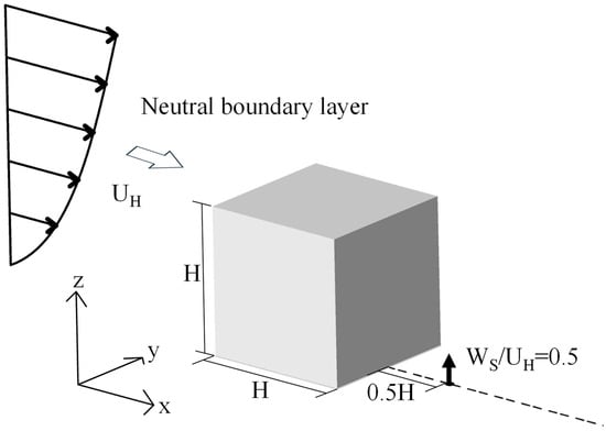
Figure 1. Schematic of the wind tunnel experiment for flow and gas dispersion around a cubic building.

The species transport equations, coupled with the SKE turbulence model, were solved to simulate the dispersion of light and heavy gas behind a cubic building. A second-order Upwind scheme was adopted for the discretization of the convection terms in the momentum equations. Pressure–velocity coupling was handled using the SIMPLE algorithm. The simulation utilized a hexahedral mesh system containing approximately 1.2 million cells. The Reynolds number (Re), based on the reference velocity U_H and the building height H was 5400. This mesh resolution is therefore considered sufficient for simulating wind flow around an isolated building at this moderate Re, as further mesh refinement was found to yield no significant improvement in the results. Figure 2 and Figure 3 present a comparison of the predicted dimensionless concentration distributions for the light and heavy gas, respectively, along three vertical lines downstream of the building (at x/H = 1.0, 1.5, and 2.0). For further validation, the LES and RANS results from Ma et al. [28], alongside the experimental data from Tominaga et al. [27], are also presented for comparison. The RANS-based CFD results from this study show close agreement with those reported by Ma et al. [28], and both align well with the trends observed in the experimental and LES data. Compared to the light gas dispersion case, the model demonstrated higher predictive accuracy for heavy gas dispersion—a finding consistent with the explanation offered by Tominaga and Stathopoulos [27]. For light gas dispersion, the RANS model slightly overestimated pollutant concentration near the ground at x/H = 1.0 and 1.5. This discrepancy may be attributed to uncertainties in the wind tunnel measurements, coupled with the inherent difficulty of RANS models in capturing the interaction between the turbulent wake and the positive buoyancy of a released light gas. A comparison of Figure 2 and Figure 3 reveals higher pollution levels for the heavy gas dispersion case. This trend was accurately reproduced by all tested CFD models. Overall, these results demonstrated that the RANS approach, when coupled with a species transport model, provides accurate predictions for the dispersion of high-buoyancy gases.

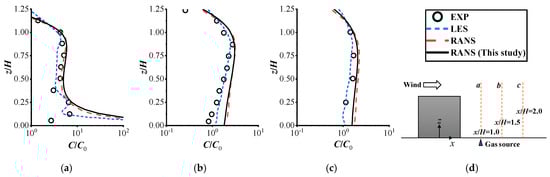
Figure 2. Vertical profiles of the dimensionless concentration C/C₀ for the light gas case at the center plane y/H = 0 behind the building: (a) x/H = 1.0; (b) x/H = 1.5; (c) x/H = 2.0; (d) positions of the vertical lines [27,28].

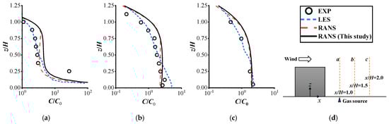
Figure 3. Vertical profiles of the dimensionless concentration C/C₀ for the heavy gas case at center plane y/H = 0 behind the building: (a) x/H = 1.0; (b) x/H = 1.5; (c) x/H = 2.0; (d) positions of the vertical lines [27,28].

4. Simulation Settings and Boundary Conditions

4.1. Simulation Arrangements

To more clearly investigate the interplay between wind and buoyancy, this study employed a 2D street canyon model to examine the resulting flow and dispersion patterns.

Kikumoto and Ooka [34] conducted wind tunnel experiments and LES on wind flow and neutral gas (C₂H₄) dispersion inside a 2D street canyon. The dimensions and geometry of the adopted street canyon model in this work were the same as those used by the above studies. Consequently, their experimental and LES results served as appropriate benchmarks for validating the present simulations. Figure 4a illustrates the 2D street canyon (or cavity) model, which has a width and height of H = 1 m, yielding an aspect ratio of 1. The canyon extends 0.3H in the spanwise direction. The computational domain above the street canyon has a vertical height of 0.2H, with upstream and downstream extensions of 0.6H each to allow for flow development. The inflow wind velocity was set to V_in = 1 m/s. The pollutants with varying plume buoyancies were released from a ground-level line source positioned at the canyon center. The source had a width of 20 mm, with the coordinate origin defined at its midpoint. All calculated concentrations were normalized by the reference concentration C* = Q/(V_in·H²), where Q is the volumetric discharge rate (m³/s).

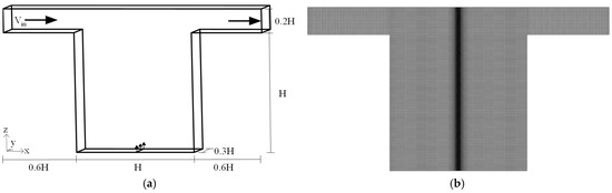
Figure 4. Geometry and mesh system of the 2D street canyon: (a) geometry; (b) mesh system (600,000).

Table 1 summarizes the six simulation cases performed in this study by solving the species transport equations. The cases are divided into two main scenarios based on pollutant discharge rate: low and high. For each scenario, light, neutral and heavy gases were considered. Ethylene (C₂H₄), with a molecular weight of 28 g/mol and a density close to that of air, was selected as the neutral gas for both scenarios. For the low-emission cases (Cases 1–3), the discharge rate was set to Q = 6 × 10⁻⁷ m³/s. Helium (He) with a molecular weight of 4 g/mol, and sulfur hexafluoride (SF₆) with a molecular weight of 146 g/mol were chosen as the light and heavy gases, respectively. These gases, with densities significantly different from air, were selected to test the performance of the passive scalar transport model under low emission conditions. For the high-emission cases (Cases 4–6), the discharge rate was increased to Q = 2.4 × 10⁻⁵ m³/s, forty times that of the low-emission cases. Methane (CH₄) with a molecular weight of 16 and carbon dioxide (CO₂) with a molecular weight of 44 served as the light and heavy gases, respectively. This set of cases was designed to examine whether significant discrepancies arise between the passive scalar and species transport models under conditions of substantial pollutant release.

Table 1. Simulation cases.

	Gas Type, Molecular Weight and Relative Density (ρp/ρa)
	Light Gas	Neutral Gas	Heavy Gas
Low emission rate Q = 6 × 10−7 m3/s	Case 1 He, 4, 0.14	Case 2 C2H4, 28, 0.97	Case 3 SF6, 146, 5.05
High emission rate Q = 2.4 × 10−5 m3/s	Case 4 CH4, 16, 0.55	Case 5 C2H4, 28, 0.97	Case 6 CO2, 44, 1.52

4.2. Boundary Conditions

The wind enters the domain from inlet with a uniform velocity of V_in = 1 m/s and a turbulence intensity of 4%. A zero-gradient condition was applied at the outlet. A symmetry conditions were adopted for the top and two side boundaries. No-slip wall boundary conditions were applied to all building surfaces, including the ground, windward wall, leeward wall, and the two roof surfaces. A pollutant with a concentration of 100% was released from the line source at two different volume flow rates: a low rate of Q = 6 × 10⁻⁷ m³/s and a high rate of Q = 2.4 × 10⁻⁵ m³/s.

Figure 4b displays the mesh systems used in this study. Hexahedral meshes were used for the simulations. The primary mesh, comprising 600,000 cells with a grid distribution of 130 × 30 × 110 in the x, y, and z directions, was applied to discretize the inner street canyon. Additionally, the gas discharge line was discretized using 10 points along the streamwise direction. The height of the first layer of fluid cells adjacent to the wall was set to 9 mm to ensure that the dimensionless wall distance, y⁺, was maintained between 20 and 50. This range satisfies the requirement for applying standard wall functions. For mesh sensitivity analysis, an additional, finer mesh system containing 1.8 million cells was generated.

Steady-state simulations were conducted employing the SKE turbulence model coupled with a species transport model. Buoyancy effects were accounted for in the k and ε equations. The air density was specified as ρ_a = 1.225 kg/m³. For the discretization of convection terms in the momentum equations, a second-order Upwind scheme was adopted. Pressure–velocity coupling was handled using the SIMPLE algorithm. Solution convergence was assumed when the residuals for all the transport equations fell below 10⁻⁶.

5. Results and Discussions

5.1. Validation of the Wind Flow and Passive Scalar Transport Model

Since the experiment conducted by Kikumoto and Ooka [34] involved the release of a neutrally buoyant gas (C₂H₄), passive scalar transport equations—which assume a constant fluid density—were first solved to validate the wind flow and pollutant concentration. Furthermore, this case was used to conduct mesh sensitivity analysis and to evaluate the performances of different turbulence models. Figure 5a compares the normalized mean streamwise velocity U/V_in along the vertical centerline at x/H = 0; Figure 5b compares the normalized mean vertical velocity W/V_in along the horizontal centerline at z/H = 0.5. Compared with wind tunnel experimental data and the LES results from Kikumoto and Ooka [34], the RANS models accurately predicted the velocity fields inside the street canyon, albeit with a slight overestimation of the wind speed. The difference between the results obtained with the SKE and the renormalisation group (RNG) k − ε models was minimal. Furthermore, compared to the results from the current mesh system (600,000 cells), those from the finer mesh system (1.8 million cells) showed no significant improvement. These findings collectively indicate that the simulation results based on the RANS approach are not sensitive to the choice of turbulence model or to the mesh density.

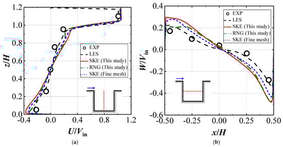
Figure 5. Comparison of normalized mean velocity profiles: (a) streamwise velocity U/V_in along the vertical centerline (x/H = 0); (b) vertical velocity W/V_in along the horizontal centerline (z/H = 0.5) [34].

Figure 6a,b shows the distributions of dimensionless concentration C/C* along the leeward wall (x/H = −0.45) and windward wall (x/H = 0.45), respectively. As expected, the concentration was higher on the leeward side and lower near the windward side—a pattern accurately captured by all CFD models. The results obtained using different RANS models and different mesh systems were nearly identical. These findings indicate that the performance of the SKE model is satisfactory for predicting both the wind flow and gas dispersion within a street canyon. Furthermore, we confirmed that the passive scalar transport model effectively simulates the dispersion of a neutrally buoyant gas. Based on these conclusions, the results obtained from the SKE model and the baseline mesh system (600,000 cells) were adopted for all subsequent studies. Finally, the concentrations predicted by the passive scalar transport model were used as a benchmark for comparison against the results from the species transport model (Cases 1–6).

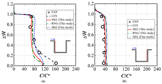
Figure 6. Comparison of normalized mean concentration C/C*: (a) along leeward side (x/H = −0.45); (b) along windward side (x/H = 0.45) [34].

5.2. Results for Low-Emission-Rate Cases

Figure 7a presents the mean streamlines and contours of dimensionless velocity magnitude U_mag/V_in for the neutrally buoyant gas dispersion case (Case 2). A comparison with the literature is valid because the release of a neutrally buoyant gas does not alter the background flow field. A large clockwise recirculation is observed inside the street canyon, with its core positioned near the center—a pattern that aligns with numerous studies of 2D street canyon flow under isothermal conditions with an aspect ratio of 1 [11,12,14,20,34]. The flow velocity throughout the canyon is generally low, approaching zero near the recirculation center. The highest velocities occur along the windward wall and near the ground. Figure 7b presents the corresponding normalized mean concentration field C/C*. Pollutant released from the floor-centered line source are blown toward the leeward side by the dominant recirculation. Consequently, elevated concentration levels are observed on the left-side ground and along the leeward wall. In contrast, concentrations remain low along the windward wall due to dilution by the incoming wind. A portion of the pollutant is transported out of the canyon through the top boundary via turbulent diffusion. For a neutrally buoyant gas, dispersion inside the canyon relies entirely on this wind-driven advection and turbulent diffusion. The flow structures and gas distribution patterns in Cases 1 and 3 are identical to those described here for Case 2.

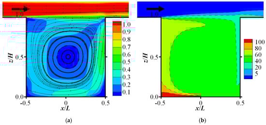
Figure 7. Distributions of mean flow and concentration fields for the low-emission-rate, neutrally buoyant gas case (Case 2, C₂H₄): (a) streamlines and contours of normalized mean velocity magnitude U_mag/V_in; (b) contours of normalized mean concentration C/C*.

Figure 8 presents the dimensionless velocity magnitude U_mag/V_in along the periphery of the street canyon (at a distance of 0.05H from the wall). For the passive scalar transport model, the density in all governing Equations (1)–(5) was treated as constant, whereas for the species transport model, it was treated as a variable. As displayed in Figure 8, the velocity magnitude distributions obtained from all CFD simulations nearly coincide. This indicates that for the low emission rates considered, the dispersion of buoyant pollutant—even with extreme variations in density—does not significantly alter the background flow field. Figure 9 compares the dimensionless mean concentration C/C* distributions along the same periphery line. The peak concentration is consistently observed near the lower leeward corner for all cases. Notably, the concentration profiles for light, neutrally buoyant, and heavy gases predicted by the species transport model are almost identical to each other and match the results from the passive scalar transport model. These findings demonstrate that, under low emission rates, the dispersion patterns and resulting concentration distributions are not sensitive to the gas type.

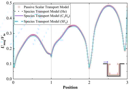
Figure 8. Normalized velocity magnitude U_mag/V_in along the building walls for all low-emission-rate cases (sampled at a distance of 0.05H from the walls).

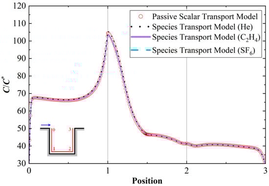
Figure 9. Normalized mean concentration C/C* along the building walls for all low-emission-rate cases (sampled at a distance of 0.05H from the walls).

Figure 10 displays the scaled density difference between the pollutant-air mixture and the ambient air, (ρ − ρ_a) × 10⁴. For Case 1 (light gas), the mixture density is lower than that of the incoming air; conversely, for Case 3 (heavy gas), it is higher. The spatial distribution of this density difference closely mirrors that of the concentration field shown in Figure 7b, with larger differences co-located with regions of higher concentration. It should be noted that the values in Figure 10 have been scaled by a factor of 10⁴; the actual density differences are therefore very small. Consequently, for the low emission rates considered, the dispersion of both light and heavy gases induces negligible change in the local fluid density. This finding is generally applicable to most pollutant dispersion scenarios within the atmospheric boundary layer. Under such conditions, the mixture density can be treated as constant. Therefore, solving the passive scalar transport equations—rather than the more complex species transport equations—represents the simplest and most efficient approach for simulating gas dispersion, even for pollutants with significant buoyancy differences.

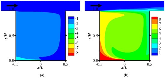
Figure 10. Scaled density difference between the mixture and ambient air (ρ − ρ_a) × 10⁴, inside the street canyon for low-emission-rate cases: (a) light gas dispersion (Case 1, He); (b) heavy gas dispersion (Case 3, SF₆).

5.3. Results for High-Emission-Rate Cases

For cases involving gas dispersion at high emission rate, methane (CH₄) served as the light gas (Case 4) and carbon dioxide (CO₂) served as the heavy gas (Case 6). The resulting single-circulation flow structure was consistent with that shown in Figure 7a. Figure 11 displays the distribution of U_mag/V_in along the periphery of the street canyon (at a distance of 0.05H from the wall) for all cases under the high emission rate conditions. Although the overall shapes of the curves are similar to those for the low emission rate cases shown in Figure 8, significant differences are evident among the CFD results. The velocity curve obtained from the passive scalar transport model overlaps with that of Case 5, which simulated the dispersion of a neutral gas (C₂H₄) by solving the species transport equation. This indicates that the dispersion of a neutral gas does not affect the flow field, regardless of the emission rate. The velocity magnitude in Case 4 is higher than that for the neutral gas because of the positive buoyancy effect caused by a light gas dispersion. Conversely, a remarkably lower wind speed is observed for the heavy gas dispersion (Case 6) because of the negative buoyancy effect, which will be discussed in a later section. These results demonstrated that the buoyancy effect induced by density difference becomes significant when a large amount of high-buoyancy gas is released.

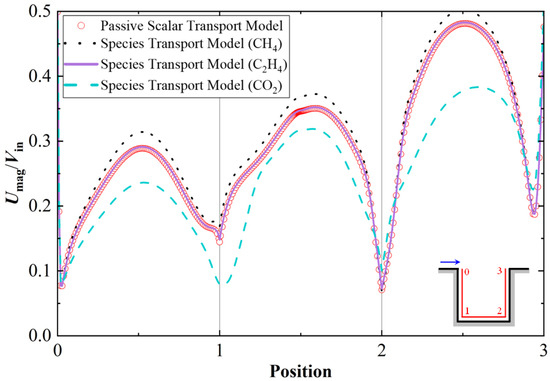
Figure 11. Distributions of the normalized mean velocity magnitude U_mag/V_in along the canyon walls for high emission cases (at a distance of 0.05H from the wall).

Figure 12 presents the dimensionless concentration distributions for Cases 4 and 6. The red and orange colors denote high-concentration zones (C/C* > 80). The extensive red and orange regions in the lower-left corner indicate that high-concentration pollutants accumulated in this area. Although the overall gas dispersion patterns are both similar to that displayed in Figure 7b, a significant difference is evident in Figure 12a,b. Compared with Case 4, much higher concentration was found near the lower-left corner in Case 6. This difference arises because the recirculation within the street canyon is enhanced when a large amount of light gas is released (Case 4), whereas it is suppressed when a large amount of heavy gases is released (Case 6). The enhanced recirculation draws more fresh air into the inner canyon, thereby diluting the polluted air.

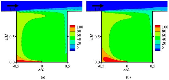
Figure 12. Contours of the normalized mean concentration C/C* for: (a) Case 4—light gas dispersion (CH₄); (b) Case 6—heavy gas dispersion (CO₂).

Figure 13 presents the near-wall concentration profiles for the three computational cases under high emission conditions. The profiles from the passive scalar transport model is included as a reference and it nearly coincided with that from Case 5. This agreement again demonstrates the effectiveness of passive scalar transport model for simulating a neutral gas dispersion, irrespective of the discharge rate. Relative to this neutral baseline, the concentration profile for the light gas (Cases 4) is significantly lower, while that for the heavy gas (Case 6) is markedly higher. The deviation is particularly pronounced for the heavy gas case.

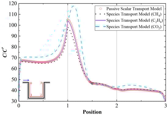
Figure 13. Normalized mean concentration C/C* along the inner walls for high-emission cases (at a distance of 0.05H from the wall).

Similarly, Figure 14 displays the density differences between the mixture and air, illustrating how much the air density was altered by the dispersion of high-buoyancy gases (the results are multiplied by 10³). The spatial distribution of this density difference closely resembles that of the concentration field in Figure 12. Consequently, the high-concentration regions correspond to areas of significant density difference. Furthermore, the magnitudes for the high-emission cases (Figure 14) are approximately ten times greater than those for the low-emission cases (Figure 10).

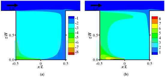
Figure 14. Contours of scaled density difference (ρ − ρ_a) × 10³ for high-emission cases: (a) Case 4—light gas dispersion (CH₄); (b) Case 6—heavy gas dispersion (CO₂).

5.4. Coupled Effects of Wind and Buoyancy Driving

The recirculation flow displayed in Figure 7a serves as the primary driving force within the street canyon, which is crucial for transporting pollutant from ground level to the top boundary. When the fluid density inside the street canyon changes, the buoyancy effect induced by density difference becomes an additional driving factor that interacts with the wind-driven flow.

As noted earlier, both thermal effect and high-buoyancy gas dispersion can alter the fluid density. In a previous study [20], we explained the interaction mechanism between wind and thermal buoyancy driving. As displayed in Figure 15a, when the ground or leeward wall is heated, the warmed air rises along the leeward wall because of its density reduction. This generates a positive buoyancy effect that can enhance the primary wind-driven recirculation. Conversely, when the windward wall is heated, as displayed in Figure 15b, thermal buoyancy exerts a negative effect.

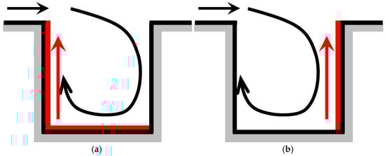
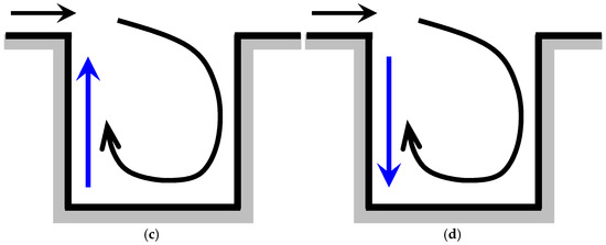
Figure 15. Mechanism of wind and buoyancy driving: (a) ground or leeward-wall heating; (b) windward-wall heating; (c) light gas dispersion; (d) heavy gas dispersion. (Panels (a,b) reproduced with permission from Ref. [20]. Copyright 2025 MDPI).

Similar to thermal buoyancy, the buoyancy effect induced by high-buoyancy gas dispersion can also either enhance or inhibit the primary recirculation, depending on the gas type. Unlike thermal buoyancy, which can manifest on either the leeward or windward side depending on which wall is heated, the buoyancy effect from pollutant dispersion always acts on the leeward side. Once a high-buoyancy gas is released from the line source, the primary recirculation transports the polluted air to the leeward side. For the light gas dispersion (Figure 15c), the low-density mixture tends to move upward, creating a positive buoyancy effect that enhances the primary recirculation. In contrast, for heavy gas dispersion (Figure 15d), the denser mixture tended to settle, generating a negative buoyancy effect that restricts the recirculation. The enhanced recirculation draws more fresh air into the street canyon, diluting the polluted air (Case 4). Conversely, restricted recirculation results in high pollution levels for the heavy gas case (Case 6).

Since the recirculation was consistently enhanced by light gas dispersion in this study, it cannot be disrupted by the release of any light gas. In contrast, heavy gas dispersion can potentially disrupt the single-recirculation flow structure if the induced negative buoyancy effect exceeds the wind-driven force. Consequently, CO₂ was selected as the heavy gas for the high-emission cases. A heavier gas such as SF₆ would not be suitable for this study, as its stronger negative buoyancy might fundamentally alter the flow regime under investigation. To maintain the one-recirculation flow pattern, both the release amount and the density of the heavy gas must be restricted. We tested release amounts larger than, and gases heavier than, CO₂; in these cases, the recirculation was completely disrupted by the negative buoyancy effect. Consequently, the oncoming wind could not enter the street canyon at all, and the entire space was filled with the heavy gas.

6. Conclusions

This study employed a validated species transport model with variable air density to investigate pollutant dispersion under varying plume buoyancies within a 2D street canyon. A passive scalar transport model was evaluated for its applicability in simulating high-buoyancy gas dispersion. Additionally, the buoyancy effects caused by the dispersion of light and heavy gases were analyzed. Based on a series of systematic numerical simulations, the following conclusions are derived:

(1) The performance of the standard k − ε model was satisfactory for predicting wind flow and gas dispersion within street canyons. The passive scalar transport model was effective for simulating neutral gas dispersion. Furthermore, the RANS approach, when coupled with the species transport model, was validated as a capable method for simulating both light and heavy gas dispersion.

(2) Under low emission rates, the dispersion of high-buoyancy pollutants only slightly altered the air density and flow field. Consequently, the concentration distributions of light, neutral, and heavy gases predicted by the species and passive scalar transport models are nearly identical.

(3) Under high emission rates, the dispersion of light and heavy gases can significantly alter the fluid density and velocity. Consequently, substantial differences emerged in the dispersion patterns of light, neutral, and heavy gases. For light and heavy gas cases, the concentrations predicted by the passive scalar transport model deviated considerably from those predicted by the species transport model.

(4) A single clockwise recirculation was observed inside the street canyon across all simulated cases, which transported the discharged pollutant to the leeward wall. The buoyancy effect from high-buoyancy gas dispersion affected the primary recirculation under high emission rates. Specifically, light gas dispersion introduced a positive buoyancy force that enhanced the recirculation, thereby reducing the pollution level within the canyon. Conversely, heavy gas dispersion generated a negative buoyancy force that restricted the wind-driven recirculation, resulting in higher pollution levels.

(5) This study demonstrated that the commonly used passive scalar transport model provides a simple and effective method for simulating neutral gas dispersion, irrespective of emission rate. It is also suitable for simulating high-buoyancy pollutant dispersion when the discharged gas quantity is insufficient to significantly alter the air density. However, the fluid density can change substantially and significant buoyancy effects can arise under high-emission scenarios. In such cases, the passive scalar transport model becomes inadequate, and the species transport model that accounts for variable fluid density must be employed to ensure accuracy.

References

- Shang, Y.; Sun, Z.; Cao, J.; Wang, X.; Zhong, L.; Bi, X.; Li, H.; Liu, W.; Zhu, T.; Huang, W. Systematic review of Chinese studies of short-term exposure to air pollution and daily mortality. Environ. Int. 2013, 54, 100–111. [Google Scholar] [CrossRef]
- Li, X.; Liu, C.; Leung, D. Large-eddy simulation of flow and pollutant dispersion in high-aspect-ratio urban street canyons with wall model. Bound.-Layer Meteorol. 2008, 129, 249–268. [Google Scholar] [CrossRef]
- Assimakopoulos, V.; ApSimon, H.; Moussiopoulos, N. A numerical study of atmospheric pollutant dispersion in different two-dimensional street canyon configurations. Atmos. Environ. 2003, 37, 4037–4049. [Google Scholar] [CrossRef]
- Huang, Y.; Hu, X.; Zeng, N. Impact of wedge-shaped roofs on airflow and pollutant dispersion inside urban street canyons. Build. Environ. 2009, 44, 2335–2347. [Google Scholar] [CrossRef]
- Gu, Z.; Zhang, Y.; Cheng, Y.; Lee, S. Effect of uneven building layout on air flow and pollutant dispersion in non-uniform street canyons. Build. Environ. 2011, 46, 2657–2665. [Google Scholar] [CrossRef]
- Kim, J.; Baik, J. Effects of inflow turbulence intensity on flow and pollutant dispersion in an urban street canyon. J. Wind Eng. Ind. Aerodyn. 2003, 91, 309–329. [Google Scholar] [CrossRef]
- Kikumoto, H.; Ooka, R. A study on air pollutant dispersion with bimolecular reactions in urban street canyons using large-eddy simulations. J. Wind Eng. Ind. Aerodyn. 2012, 104–106, 516–522. [Google Scholar] [CrossRef]
- Gromke, C.; Ruck, B. Influence of trees on the dispersion of pollutants in an urban street canyon-Experimental investigation of the flow and concentration field. Atmos. Environ. 2007, 41, 3287–3302. [Google Scholar] [CrossRef]
- Uehara, K.; Murakami, S.; Oikawa, S.; Wakamatsu, S. Wind tunnel experiments on how thermal stratification affects flow in and above urban street canyons. Atmos. Environ. 2000, 34, 1553–1562. [Google Scholar] [CrossRef]
- Allegrini, J.; Dorer, V.; Carmeliet, J. Wind tunnel measurements of buoyant flows in street canyons. Build. Environ. 2013, 59, 315–326. [Google Scholar] [CrossRef]
- Xie, X.; Liu, C.; Leung, D. Impact of building facades and ground heating on wind flow and pollutant transport in street canyons. Atmos. Environ. 2007, 41, 9030–9049. [Google Scholar] [CrossRef]
- Cheng, W.; Liu, C. Large-eddy simulation of turbulent transports in urban street canyons in different thermal stabilities. J. Wind Eng. Ind. Aerod. 2011, 99, 434–442. [Google Scholar] [CrossRef]
- Cai, X. Effects of differential wall heating in street canyons on dispersion and ventilation characteristics of a passive scalar. Atmos. Environ. 2012, 51, 268–277. [Google Scholar] [CrossRef]
- Li, X.; Britter, R.; Norford, L.; Koh, T.; Entekhabi, D. Flow and pollutant transport in urban street canyons of different aspect ratios with ground heating: Large-eddy simulation. Bound.-Layer Meteorol. 2012, 142, 289–304. [Google Scholar] [CrossRef]
- Jiang, G.; Yoshie, R. Large-eddy simulation of flow and pollutant dispersion in a 3D urban street model located in an unstable boundary layer. Build. Environ. 2018, 142, 47–57. [Google Scholar] [CrossRef]
- Jiang, G.; Hu, T.; Yang, H. Effects of Ground Heating on Ventilation and Pollutant Transport in Three-Dimensional Urban Street Canyons with Unit Aspect Ratio. Atmosphere 2019, 10, 286. [Google Scholar] [CrossRef]
- Chen, L.; Hang, J.; Chen, G.; Liu, S.; Lin, Y.; Mattsson, M.; Sandberg, M.; Ling, H. Numerical investigations of wind and thermal environment in 2D scaled street canyons with various aspect ratios and solar wall heating. Build. Environ. 2021, 190, 107525. [Google Scholar] [CrossRef]
- Cui, P.; Ji, R.; He, L.; Zhang, Z.; Luo, Y.; Yang, Y.; Huang, Y. Influence of GI configurations and wall thermal effects on flow structure and pollutant dispersion within urban street canyons. Build. Environ. 2023, 243, 110646. [Google Scholar] [CrossRef]
- Mei, S.; Yuan, C. Urban buoyancy-driven air flow and modelling method: A critical review. Build. Environ. 2022, 210, 108708. [Google Scholar] [CrossRef]
- Jiang, G.; Wu, M.; Li, H.; Wu, Y. Mechanism of Wind and Buoyancy Driving on Ventilation and Pollutant Transport in an Idealized Urban Street Canyon. Buildings 2024, 14, 3168. [Google Scholar] [CrossRef]
- Milliez, M.; Carissimo, B. Numerical simulations of pollutant dispersion in an idealized urban area, for different meteorological conditions. Bound.-Layer Meteorol. 2007, 122, 321–342. [Google Scholar] [CrossRef]
- Hanna, S.; Tickle, G.; Mazzola, T.; Gant, S. Dense gas plume rise and touchdown for Jack Rabbit II trial 8 chlorine field experiment. Atmos. Environ. 2021, 260, 118551. [Google Scholar]
- Lin, C.; Ooka, R.; Kikumoto, H.; Sato, T.; Arai, M. Wind tunnel experiment on high-buoyancy gas dispersion around isolated cubic building. J. Wind Eng. Ind. Aerodyn. 2020, 202, 104226. [Google Scholar] [CrossRef]
- Tominaga, Y.; Stathopoulos, T. Ten questions concerning modeling of near-field pollutant dispersion in the built environment. Build. Environ. 2016, 105, 390–402. [Google Scholar] [CrossRef]
- Olvera, H.; Choudhuri, A.; Li, W. Effects of plume buoyancy and momentum on the near-wake flow structure and dispersion behind an idealized building. J. Wind Eng. Ind. Aerodyn. 2008, 96, 209–228. [Google Scholar] [CrossRef]
- Mokhtarzadeh-Dehghan, M.; Akcayoglu, A.; Robins, A. Numerical study and comparison with experiment of dispersion of a heavier-than-air gas in a simulated neutral atmospheric boundary layer. J. Wind Eng. Ind. Aerodyn. 2012, 110, 10–24. [Google Scholar] [CrossRef]
- Tominaga, Y.; Stathopoulos, T. CFD simulations of near-field pollutant dispersion with different plume buoyancies. Build. Environ. 2018, 131, 128–139. [Google Scholar] [CrossRef]
- Ma, H.; Zhou, X.; Tominaga, Y.; Gu, M. CFD simulation of flow fields and pollutant dispersion around a cubic building considering the effect of plume buoyancies. Build. Environ. 2022, 208, 108640. [Google Scholar] [CrossRef]
- Rossi, R.; Philips, D.; Iaccarino, G. A numerical study of scalar dispersion downstream of a wall-mounted cube using direct simulations and algebraic flux models. Int. J. Heat Fluid Flow 2010, 31, 805–819. [Google Scholar] [CrossRef]
- Tominaga, Y.; Stathopoulos, T. Numerical simulation of dispersion around an isolated cubic building: Model evaluation of RANS and LES. Build. Environ. 2010, 45, 2231–2239. [Google Scholar] [CrossRef]
- Tominaga, Y.; Stathopoulos, T. CFD modeling of pollution dispersion in a street canyon: Comparison between LES and RANS. J. Wind Eng. Ind. Aerodyn. 2011, 99, 340–348. [Google Scholar] [CrossRef]
- Rossi, R.; Iaccarino, G. Numerical analysis and modeling of plume meandering in passive scalar dispersion downstream of a wall-mounted cube. Int. J. Heat Fluid Flow 2013, 43, 137–148. [Google Scholar] [CrossRef]
- Ai, Z.; Mak, C. Analysis of fluctuating characteristics of wind-induced airflow through a single opening using LES modeling and the tracer gas technique. Build. Environ. 2014, 80, 249–258. [Google Scholar] [CrossRef]
- Kikumoto, H.; Ooka, R. Large-eddy simulation of pollutant dispersion in a cavity at fine grid resolutions. Build. Environ. 2018, 127, 127–137. [Google Scholar] [CrossRef]
- Jiang, G.; Yoshie, R. Side ratio effects on flow and pollutant dispersion around an isolated high-rise building in a turbulent boundary layer. Build. Environ. 2020, 180, 107078. [Google Scholar] [CrossRef]
- Zheng, X.; Yang, J. Impact of moving traffic on pollutant transport in street canyons under perpendicular winds: A CFD analysis using large-eddy simulations. Sustain. Cities Soc. 2022, 82, 103911. [Google Scholar] [CrossRef]
- Jiang, G.; Wu, M.; Hu, T. Turbulence and Pollutant Statistics around a High-Rise Building with and without Overhangs. Atmosphere 2023, 14, 1771. [Google Scholar] [CrossRef]
- Cao, G.; Hu, T.; Jiang, G.; Cao, J.; Liu, Y. Effect of building parameters on urban ventilation efficiency for pedestrian areas: Considering internal and external pollution sources. J. Wind Eng. Ind. Aerodyn. 2025, 264, 106150. [Google Scholar] [CrossRef]
- Klippel, K.; Goulart, V.; Auerswald, T.; Galvao, E.; Ciarelli, P.; Reis, N.C., Jr.; Coceal, O. Spatial patterns of probability distributions for concentration fluctuations at the street network scale. Build. Environ. 2025, 285, 113491. [Google Scholar] [CrossRef]
- Salim, S.; Cheah, S.; Chan, A. Numerical simulation of dispersion in urban street canyons with avenue-like tree plantings: Comparison between RANS and LES. Build. Environ. 2011, 46, 1735–1746. [Google Scholar] [CrossRef]
- Nejat, P.; Calautit, J.; Majid, M.; Hughes, B.; Jomehzadeh, F. Anti-short-circuit device: A new solution for short-circuiting in windcatcher and improvement of natural ventilation performance. Build. Environ. 2016, 105, 24–39. [Google Scholar] [CrossRef]
- Mei, S.; Zhao, Y.; Talwar, T.; Carmeliet, J.; Yuan, C. Neighborhood scale traffic pollutant dispersion subject to different wind-buoyancy ratios: A LES case study in Singapore. Build. Environ. 2023, 228, 109831. [Google Scholar] [CrossRef]
Disclaimer/Publisher’s Note: The statements, opinions and data contained in all publications are solely those of the individual author(s) and contributor(s) and not of MDPI and/or the editor(s). MDPI and/or the editor(s) disclaim responsibility for any injury to people or property resulting from any ideas, methods, instructions or products referred to in the content. |
© 2025 by the authors. Licensee MDPI, Basel, Switzerland. This article is an open access article distributed under the terms and conditions of the Creative Commons Attribution (CC BY) license.