Construction of a Model for Estimating PM_2.5 Concentration in the Yangtze River Delta Urban Agglomeration Based on Missing Value Interpolation of Satellite AOD Data and a Machine Learning Algorithm

Abstract

Air pollution is an important environmental issue that affects social development and human life. Atmospheric fine particulate matter (PM_2.5) is the primary pollutant affecting the air quality of most cities in the authors’ country. It can cause severe haze, reduce air visibility and cleanliness, and affect people’s daily lives and health. Therefore, it has become a primary research object. Ground monitoring and satellite remote sensing are currently the main ways to obtain PM_2.5 data. Satellite remote sensing technology has the advantages of macro-scale, dynamic, and real-time functioning, which can make up for the limitations of the uneven distribution and high cost of ground monitoring stations. Therefore, it provides an effective means to establish a mathematical model—based on atmospheric aerosol optical thickness data obtained through satellite remote sensing and PM_2.5 concentration data measured by ground monitoring stations—in order to estimate the PM_2.5 concentration and temporal and spatial distribution. This study takes the Yangtze River Delta region as the research area. Based on the measured PM_2.5 concentration data obtained from 184 ground monitoring stations in 2023, the newly released sixth version of the MODIS aerosol optical depth product obtained via the US Terra and Aqua satellites is used as the main prediction factor. Dark-pixel AOD data with a 3 km resolution and dark-blue AOD data with a 10 km resolution are combined with the European Center for Medium-Range Weather Forecasts (ECMWF) reanalysis meteorological, land use, road network, and population density data and other auxiliary prediction factors, and XGBoost and LSTM models are used to achieve high-precision estimation of the spatiotemporal changes in PM_2.5 concentration in the Yangtze River Delta region.

1. Introduction

With the rapid development of China’s economy, the construction of new rural areas is constantly being promoted. Green land is decreasing, urban buildings are increasing, population distribution is becoming more concentrated, and automobile exhaust is being discharged in large quantities, resulting in frequent air pollution incidents. As such, urban air quality has become a hot topic. PM_2.5 (fine atmospheric particulate matter with an aerodynamic diameter of less than 2.5 microns) is an important indicator that can reflect the air quality status, and has attracted particular attention. Compared with PM10 (inhalable particulate matter with an aerodynamic diameter of less than 10 microns), PM_2.5 has a smaller particle size and a larger surface area, making it easier for it to adsorb surrounding toxic substances, heavy metals, and so on; furthermore, it has a longer transmission distance, stays in the atmosphere for a longer time, and can enter the alveolar terminal and even the blood circulation through human breathing. A large number of studies have shown that PM_2.5 has impacts on air quality, human health, the ecological environment, visibility, climate change, economic development, and many other aspects [1]. For example, PM_2.5 causes damage to the respiratory system, triggers lung inflammation, and is even related to gene mutations [2,3]. Particles of varying sizes in the air can also reduce air visibility to varying degrees. PM_2.5 has a much greater weakening effect on visible light than other particles, and is the main factor affecting visibility [4]. Hazy weather can affect people’s normal lives, which is mainly caused by tiny particles emitted from anthropogenic sources into the atmosphere, which disperse into the atmosphere to form solid aerosols called haze. Fine particles of PM_2.5 in the atmosphere are key pollutants in the formation of haze [5]. Severe haze can reduce visibility and cause inconvenience in people’s travel and transportation. In addition, the scattering and absorption of solar radiation by PM_2.5 is also expected to affect global climate change [6]. In addition, high concentrations of PM2.5 can cause serious social and economic losses. It has been estimated that, in 2010, the economic losses caused by PM_2.5 pollution in the Yangtze River Delta region were about 22.1 billion yuan while, in 2012, PM_2.5 pollution in Beijing, Shanghai, and other places caused economic losses of about 6.82 billion yuan [7,8]. Song Y. et al. [9] evaluated the direct economic losses caused by large-scale smog events and found that during January 2013, severe PM_2.5 pollution caused direct economic losses of about 23 billion yuan relating to the transportation and health sectors across the country, accounting for 98% of the total losses. It can be seen that obtaining timely and accurate PM_2.5 concentration data and its spatiotemporal distribution characteristics can provide important reference value for climate change research, health damage predictions, economic loss assessments, and so on. There are two main ways to obtain PM_2.5 concentration data: ground monitoring and satellite remote sensing. Conventional ground monitoring involves establishing ground monitoring stations for continuous observation. Since 2013, China has successively established a PM_2.5 monitoring network covering the whole country. As of 2023, the number of PM_2.5 monitoring stations reached 1497, and it is currently the country with the most atmospheric monitoring stations in the world [10]. Although ground monitoring stations can collect real-time data on PM_2.5 concentration in a timely and accurate manner, this method has the disadvantages of a limited number of stations, a high cost of station construction, and an uneven spatial distribution. Compared with traditional monitoring methods, satellite remote sensing can further make up for the shortcomings of ground monitoring sites. Through quantitative inversion of satellite remote sensing images, PM_2.5 concentration data with a wider range, higher resolution, and longer continuous observation time can be obtained. In addition, through satellite observation, the transmission path and distribution characteristics of pollutants, the location of pollution sources, and even the global pollution status and air quality changes can be obtained [11]. Aerosol refers to the general term for solid and gaseous particles suspended in the air with a diameter between 0.001 and 100 μm. Aerosol Optical Depth (AOD) refers to the integral of the extinction coefficient of particulate matter in the vertical column of the entire atmosphere under cloudless conditions. It is used to describe the weakening effect of aerosols on solar radiation and can reflect the turbidity of the atmosphere. AOD is a dimensionless quantity. Kahn et al. used a Multi angle Imaging Spectroradiometer (MISR) to study aerosols in the ocean air. The results showed that the particle size range corresponding to AOD inversion in the visible near-infrared spectral band was between 0.1 and 2 microns, which was close to the diameter range of PM_2.5 particles. This provides a theoretical basis for AOD inversion of PM_2.5. Therefore, using remote sensing technology to invert high-resolution PM_2.5 concentration data in urban areas and at larger scales has important practical significance. In order to achieve effective understanding and control of PM_2.5 in the Yangtze River Delta urban agglomeration in China and realize the detailed spatio-temporal quantification of PM_2.5, this study takes the Yangtze River Delta region of China as the research area, and uses the PM_2.5 hourly concentration data obtained by 184 ground monitoring stations in 2023 and the sixth version of the MODIS aerosol optical thickness products which have been newly released by NASA based on the Terra and Aqua satellites, including DT AOD data with a 3 km resolution obtained using the Dark Target (DT) algorithm and DB AOD data with a 10 km resolution obtained using the Deep Blue (DB) algorithm. Although MODIS 3 km dark pixel AOD and 10 km deep blue AOD have the following obvious limitations: a large number of pixels are missing in cloud and high aerosol optical thickness scenes, resulting in a reduction in effective observation days by about 30–50%; Only two crossings per day (Terra, Aqua), with insufficient time resolution to analyze short-term pollution outbreaks; The spatial resolutions of 3 km and 10 km may still mix multiple emission sources within the city, resulting in “same pixel, different source” errors; AOD–PM_2.5. The conversion requires the introduction of assumptions such as aerosol vertical profiles and humidity, as regional differences can amplify inversion uncertainty; There are few AERONET foundation verification sites in the Yangtze River Delta region, which limits direct cross validation. The main reason for choosing this data in this article is that MODIS products are long time series (>20 years) AOD data that simultaneously cover the entire Yangtze River Delta region (≥350,000 km²) and have a resolution of 3 km near urban scale, which can compensate for 124 ground PM_2.5 The problem of uneven distribution of site space; The C6.1 version of the Dark Pixel and Deep Blue algorithm has been systematically validated in different climate zones around the world, with clear error characteristics, making it easy to compensate for errors in the model through “missing pixel labeling + spatiotemporal weighted interpolation”; Combining ECMWF reanalysis with high-resolution auxiliary variables such as 1 km level land use and road network can effectively reduce spatial mixing errors in statistical models. Therefore, after weighing “coverage, spatiotemporal resolution, algorithm availability” and “known error controllability”, MODIS 3 km/10 km AOD is still the current condition for conducting PM_2.5 in the Yangtze River Delta region The optimal publicly available data source for high-precision spatiotemporal estimation. Based on the linear relationship between the AOD data of the two satellites and the respective advantages of the two data products, linear interpolation is used to fill in the areas where AOD data are missing. The fused AOD is used as the main prediction factor, combined with the reanalysis meteorological data from the European Center for Medium-Term Meteorological Forecasts (ECMWF), as well as population density, land use, and other auxiliary prediction factors. Spearman rank correlation analysis is performed to explore the key factors affecting the changes in the spatiotemporal distribution of PM_2.5 concentrations. The Extreme Gradient Boosting (XGBoost) model and the long short-term memory (LSTM) model are used, and the prediction results of the two models are compared and analyzed to achieve high-precision estimation of the spatiotemporal changes in PM_2.5 concentration in the Yangtze River Delta region. A flowchart of the research is shown in Figure 1.

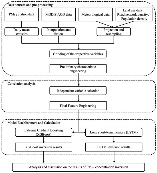
Figure 1. The research flowchart.

In recent years, the research on the estimation of the concentration of PM_2.5 has mostly relied on the traditional linear or shallow machine learning model, which has difficulty in capturing its complex nonlinear dynamics and long time-series dependence at the same time. Xgboost and LSTM break through this bottleneck from the two complementary perspectives of “feature interaction” and “time memory”, respectively: xgboost, based on the idea of boosting integration, constructs high-order nonlinear maps through layer by layer splitting, and has natural advantages for complex interactions between multi-source heterogeneous variables (satellite AOD, meteorology, LUCC, etc.). It can output feature importance to identify key drivers, and maintain excellent generalization ability in small to medium samples; By virtue of gating mechanism and memory unit, LSTM can depict PM_2.5 The accumulation, lag and periodic changes in the long time series effectively integrate the temporal dynamics of the reanalysis data of the meteorological field, and make up for the lack of xgboost in describing the “time dimension”. The combination of the two can not only analyze the “space attribute” nonlinear relationship, but also track the “time memory” evolution process, providing a more accurate and more explanatory estimation framework for the Yangtze River Delta, a region with complex meteorological emission transport mechanism and highly time-varying pollution process.

2. Data and Methods

2.1. Study Area

The Yangtze River Delta region is located on the eastern coast of China and is in an important position in the Asia-Pacific Economic Zone. It is one of the most important urban agglomerations in China and one of the regions with the fastest economic development, the highest degree of openness, the strongest innovation capabilities, and the largest number of immigrants. In 2018, the total GDP of the 25 cities in the Yangtze River Delta was approximately 17.8 trillion yuan [12]. Due to its superior location and strong industry, this rapid economic growth is also accompanied by the pressure of deteriorating environmental quality. According to the “Regional Plan for the Yangtze River Delta Region” [13], officially approved and implemented by the State Council on 24 May 2010, the Yangtze River Delta region includes Shanghai, Jiangsu Province, and Zhejiang Province, with a regional area of 211,700 square kilometers and a population of 150 million. The regional plan divides 25 cities in Shanghai, Jiangsu, and Zhejiang into core areas and radiation areas. The 16 core area cities include Shanghai, Nanjing, Hangzhou, Suzhou, Wuxi, Ningbo, Taizhou, Yangzhou, Zhenjiang, Nantong, Changzhou, Huzhou, Jiaxing, Shaoxing, Zhoushan, and Taizhou, with an area range of 118.33 E ~ 122.95 E and 29.04 N ~ 33.41 N.

2.2. Data Sources

The hourly updated ground PM_2.5 concentration data used in this study were derived from the hourly concentration values and 24 h concentration averages released in real time by the China Environmental Monitoring Center (CEMC) through the “National Urban Air Quality Real-time Release Platform” (https://www.sysu.edu.cn/newsen/info/1701/55691.htm, accessed on 26 October 2025). The ground PM_2.5 concentration data are obtained by monitoring using the micro-oscillating balance method, also known as the β-ray method. For our study, the hourly PM_2.5 concentration data for each monitoring station for the 365 days from 1 January to 31 December 2023 were downloaded. The research area covers 16 prefecture-level cities, 117 county-level cities, and 184 ground-based monitoring stations in the Yangtze River Delta region. The distribution of the research area and stations is shown in Figure 2.

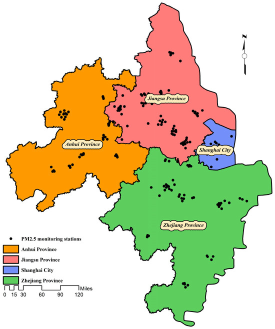
Figure 2. Study area and PM_2.5 monitoring station distribution map.

The MODIS AOD data used in this study were the C6 version of aerosol products downloaded from the LAADS (Level-1 Atmosphere Archive and Distribution System) website (https://ladsweb.modaps.eosdis.nasa.gov/, accessed on 26 October 2025), including AOD with a resolution of 3 km (M*D04-3K) and AOD with a resolution of 10 km (M*D04-L2), where “*” denotes “O” and “Y” (which stand for Terra and Aqua, respectively). The downloaded data were all in the HDF layered data format, and the remote sensing image processing software ENVI5.6 was used for unified projection and format conversion to obtain geotiff format files with a projection coordinate system of WGS-1984.

The reanalysis meteorological data of the European Center for Medium-Range Weather Forecasts (ECMWF) (https://apps.ecmwf.int/datasets/ (accessed 1 March 2024)) were used, including the temperature at 2 m above the ground (T_2m, K), the meridional wind speed (V₁₀, m/s, V is positive when the wind direction is south and negative when the wind direction is north), the zonal wind speed (U₁₀, m/s, U is positive when the wind direction is west and negative when the wind direction is east), the boundary layer height (PBL, m), the relative humidity near the ground (RH, %), and the atmospheric pressure (P, Pa).

The national land use data product of 2020 with a spatial resolution of 1 km was used, which was obtained from the Ministry of Land and Resources. The land use types include 6 primary types and 25 secondary types. According to the needs of the study, the ArcMap 10.8 software was used to extract and calculate the cultivated land, urban and rural land, industrial and mining land, and residential land in the primary classification in the study area. The secondary classification is paddy fields, dry land, urban land, rural settlements, and other construction land (factories, mines, large industrial areas, transportation roads, airports, etc., independent of towns).

The road data for the Yangtze River Delta region were obtained as spatial distribution vector data of roads in the country, which were downloaded from the Geographic National Conditions Monitoring Platform (http://www.dsac.cn/DataProduct/Index/200804, accessed on 26 October 2025). For this study, the road network density of national roads, provincial roads, county roads, urban roads, and expressways was calculated in a 3 km × 3 km grid (unit: km/km²). The population density data were obtained from the 2020 national census (unit: person/km²).

2.3. Data Preprocessing

In combining the 3 km DT AOD and 10 km DB AOD products of Aqua and Terra, the missing AOD data are filled in through the following three steps.

• The daily Aqua and Terra DT AOD data were matched in time and space, and the linear relationship between the two was analyzed. The daily correlation coefficient R value was calculated to be between 0.60 and 0.98, indicating that there is a good linear correlation between the two data products. The missing AOD values on the grid were filled through linear interpolation between the available data points. The calculation formula is as follows:

  $$\begin{array}{c}{AOD}_{A mis}={\alpha }_1+{\beta }_1{AOD}_{Terra}\end{array}$$

  (1)

  $$\begin{array}{c}{AOD}_{T mis}={\alpha }_2+{\beta }_2{AOD}_{Aqua}\end{array}$$

  (2)

  where ${AOD}_{A mis}$ and ${AOD}_{T mis}$ represent the missing Aqua and Terra AOD values, respectively; ${\alpha }_1$ and ${\alpha }_2$ are intercepts; and ${\beta }_1$ and ${\beta }_2$ are slopes that are calculated by establishing a linear relationship between the non-missing Aqua and Terra AOD values. When Aqua AOD data are missing, Formula (1) is used to calculate the missing AOD value; when Terra AOD is missing, Formula (2) is used to calculate the missing AOD value.
• The cubic convolution method provided by the ENVI remote sensing processing software was used to resample the DB AOD data of Aqua and Terra with a resolution of 10 km to a resolution of 3 km. The sampling rate is 0.3. The resampled DB AOD data were processed in the same way as in step 1.
• The linearly interpolated DT AOD was fused with the BD AOD; that is, the grid was filled with DB AOD where the DT AOD data were missing.

Taking the AOD product from 1 June 2023 as an example, Figure 3 show the processing results of the above fusion method.

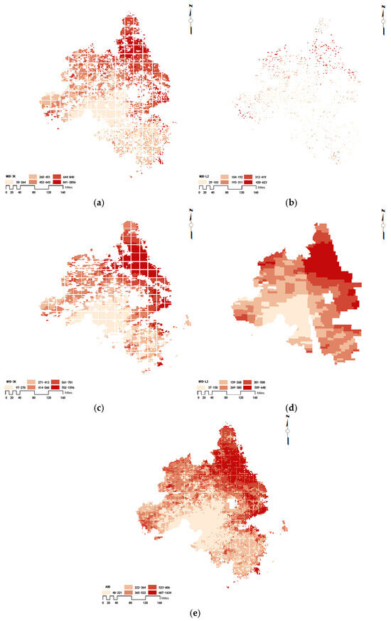
Figure 3. Results of AOD filling and fusion in the Yangtze River Delta region on 1 June 2023: (a) Aqua 3 km DT AOD; (b) Aqua 10 km DB AOD; (c) Terra 3 km DT AOD; (d) Terra 10 km DB AOD; (e) AOD interpolation and fusion results.

When performing spatiotemporal matching, the consistency of all data in time and space should be ensured as much as possible. The resolution of the AOD data after interpolation and fusion was 3 km × 3 km. In order to match with the AOD data, the Fishnet tool in the ArcGIS 10.8.2 software was used in this study to create 27,333 grids with a resolution of 3 km × 3 km for the entire study area. Then, AOD, meteorological elements, population density, land use (paddy fields, dry land, urban land, rural residential areas, and other construction land) area proportions, and road network density (national highways, provincial highways, county roads, expressways, and urban roads) were extracted for the 3 km × 3 km grids. With the grid where a PM_2.5 ground monitoring station is located as the center, the average value of each independent variable data in the 3 × 3 (81 km²) grids around the grid center was calculated and then spatially matched with the PM_2.5 concentration data. The temporal matching was based on date matching. The processing results for each variable are shown in Figure 4 and Figure 5.

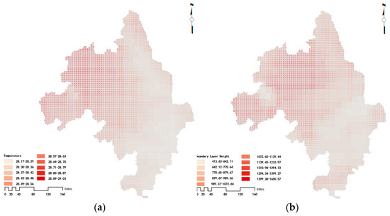
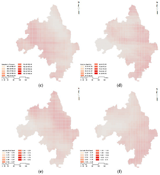
Figure 4. Results of the extraction of meteorological data in the Yangtze River Delta region on 1 June 2023: (a) temperature; (b) boundary layer height; (c) atmospheric pressure; (d) relative humidity; (e) longitudinal wind speed; (f) latitudinal wind speed.

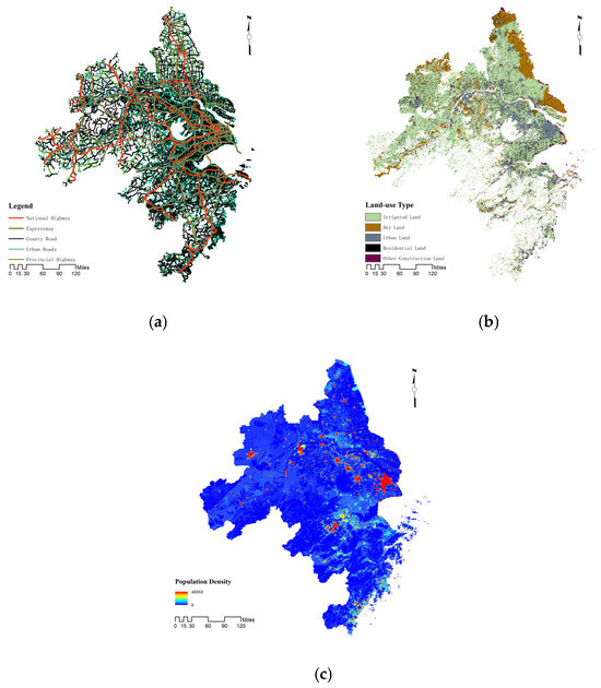
Figure 5. Preprocessing results for other independent variables: (a) Road network distribution in the Yangtze River Delta region in 2020; (b) land use distribution in the AOD filling and fusion results in the Yangtze River Delta region in 2023; (c) population density of the Yangtze River Delta region in 2020.

2.4. Research Methods

2.4.1. Correlation Analysis

For the grid data that were matched in time and space, Spearman correlation analysis was performed using the daily average PM_2.5 concentration data from the stations as the dependent variable and the remaining variables as independent variables. The correlation analysis results between PM_2.5 and various variables are shown in Table 1 and Table 2.

Table 1. Analysis results of the correlation between PM_2.5, AOD, and meteorological elements.

Variant	T AOD	A AOD	T	BLH	Pa	U	V	RH
Correlation Coefficient	0.532 **	0.536 **	−0.703 **	−0.415 **	0.442 **	−0.459 **	0.628 **	−0.545 **

** When the confidence level (two-sided) is 0.01, the correlation is significant.

Table 2. Correlation analysis results between PM_2.5 and other elements.

Variant	National Roads	Provincial Roads	County Roads	Expressways	Urban Land	Paddy Fields	Dry Land	Urban Land	Rural Settlements	Other Construction Land
Correlation Coefficient	0.190 *	0.222 *	0.258 **	0.357 **	0.207 *	0.218 *	0.300 **	0.223 *	0.331 **	0.269 **

** When the confidence level (two-sided) is 0.01, the correlation is significant, * When the confidence level (two-sided) is 0.05, the correlation is significant.

2.4.2. XGBoost Model

In this study, the XGBoost (Extreme Gradient Boosting) model algorithm was used for the fitting and prediction of time-series data, and the influence of each variable on the dependent variable was deeply analyzed and evaluated. XGBoost is an efficient machine learning method based on the gradient boosting framework. Its core idea is to gradually build a series of weak learners (usually decision trees) through an additive model and optimize the loss function through each step of gradient descent to finally form a powerful integrated model. Compared with traditional machine learning algorithms, the XGBoost model has excellent computational efficiency and generalization ability, and is particularly suitable for processing large-scale and complex time-series datasets.

The XGBoost model is particularly widely used with time-series data. It can predict future trends by modeling the complex nonlinear relationships between independent variables in the time dimension. When processing time-series data, the XGBoost algorithm effectively improves the fitting performance of the model through parallel computing and refined loss function optimization [14]. The algorithm also has the advantages of handling missing values, custom objective functions, and automatic feature selection, making it more robust in the prediction of time-series data [15]. Unlike linear models, the XGBoost model’s predictions not only rely on the input information at the current moment, but can also capture multi-dimensional feature interactions [16]. By combining multiple decision trees, the XGBoost model can effectively extract hidden patterns and trends in time-series data, improving the prediction accuracy of the model. In addition, XGBoost has built-in L1 and L2 regularization terms to prevent the model from overfitting and enhance its generalization ability on future data [17].

In the process of studying the fitting process, the XGBoost model also provides an evaluation mechanism for the degree to which each selected independent variable affects the dependent variable. Specifically, the XGBoost model can measure the role of each independent variable in the model through feature importance analysis. Feature importance is usually evaluated based on the gain value at the time of node splitting or the number of times a feature appears [18]. In this study, we used a gain-based feature importance analysis method to conduct a detailed evaluation of the impact of each independent variable on the target variable. This method helps to clearly identify the features that play key roles in the prediction of the dependent variable and those that contribute less to the model, which helps to further optimize the model and improve the prediction accuracy.

In the specific calculation process, the XGBoost Model minimizes the loss function by gradually fitting each base learner. In each round of iteration, the algorithm generates a new decision tree based on the residuals of the previous round to learn from these errors. Finally, by integrating multiple decision trees, the XGBoost Model achieves accurate fitting and prediction of time-series data. In this study, the model can not only fit the existing historical data but also effectively predicts future trend changes, which makes the XGBoost model an important tool for processing time-series data prediction tasks.

In addition, the XGBoost model is also used in this study to evaluate the complex dependencies between the independent and dependent variables. Through feature importance analysis, we can understand which independent variables play a key role in the prediction process of the model. The results of feature importance analysis provide us with valuable explanatory information, which helps to further understand the dynamic structure of time-series data and the relative importance of independent variables.

In order to improve the prediction performance of the model and optimize parameter selection, the XGBoost Model aims to minimize the loss function by iteratively constructing decision trees [19]. The goal of the XGBoost Model is to minimize the loss function L(θ), which is expressed as

$$\begin{array}{c}L\left(\theta \right)={\displaystyle \sum _{i=1}^n}l\left(y_i,{\widehat{y}}_i\right)+{\displaystyle \sum _{k=1}^K}\Omega \left(f_k\right)\end{array}$$

(3)

where $l\left(y_i,{\widehat{y}}_i\right)$ is the loss function, which is used to measure the difference between the true value $y_i$ and the predicted value $y_i$. The square error or logarithmic loss function is usually chosen [20]. $\Omega \left(f_k\right)$ is the regularization term, which is defined as

$$\begin{array}{c}\Omega \left(f_k\right)=\gamma T+{\displaystyle \frac{1}{2}}\lambda {\displaystyle \sum _j}{\omega }_j^2\end{array}$$

(4)

where $T$ is the number of leaf nodes in the tree, $\gamma$ is the regularization parameter, and ${\omega }_j^2$ is the weight of the leaf node. By introducing the regularization term, overfitting of the model can effectively be prevented [21].

The core of XGBoost is the learning of residuals. In each round of iteration, XGBoost builds a new decision tree based on the prediction residuals of the previous round [22]. Assuming that the prediction value of round $t$ is ${\widehat{y}}_i^{\left(t\right)}$, its calculation formula is

$$\begin{array}{c}{\widehat{y}}_i^{\left(t\right)}={\widehat{y}}_i^{\left(t-1\right)}+f_t\left(x_i\right)\end{array}$$

(5)

In this section, where applicable, the authors are required to disclose details of how generative artificial intelligence (GenAI) has been used in this paper (e.g., to generate text, data, or graphics, or to assist in study design, data collection, analysis, or interpretation). The use of GenAI for superficial text editing (e.g., grammar, spelling, punctuation, and formatting) does not need to be declared.

Here, $f_t\left(x_i\right)$ is the prediction given by tree $t$. To update the model parameters, XGBoost approximates the objective function using a second-order Taylor expansion as follows:

$$\begin{array}{c}{L}^{\left(t\right)}\approx {\displaystyle \sum _{i=1}^n}\left[g_i{f}_t\left(x_i\right)+{\displaystyle \frac{1}{2}}{h}_i{f}_t{\left(x_i\right)}^2\right]+\Omega \left(f_t\right)\end{array}$$

(6)

Here, $g_i$ and $h_i$ are the first-order and second-order derivatives; namely, the gradient and Hessian matrix, respectively. By minimizing this approximate loss, XGBoost can effectively update the model parameters [23].

XGBoost not only performs well in fitting and predicting time-series data, but also provides analysis tools for the importance of each variable. In feature importance analysis, the importance of a feature can be measured by the split gain; that is, the contribution of a feature to the reduction in the loss function when the tree splits the node [24]. Specifically, for each feature $x_i$, its importance can be expressed as

$$\begin{array}{c}Importance\left(x_j\right)={\displaystyle \sum _{nodes split on x_j}}Gain\end{array}$$

(7)

In addition, XGBoost also introduces a learning rate $\eta$ and subsampling strategy to further improve the robustness of the model. The introduction of the learning rate can alleviate the problem of excessive gradient updates during model training and make the model convergence more stable [25]. The adjustment formula for the learning rate $\eta$ is

$$\begin{array}{c}{\widehat{y}}_i^{\left(t\right)}={\widehat{y}}_i^{\left(t-1\right)}+\eta f_t\left(x_i\right)\end{array}$$

(8)

The subsampling strategy reduces the variance of the model and further reduces the risk of overfitting by randomly selecting a subset of features and data for training.

In this study, XGBoost was not only successfully used for fitting and predicting time-series data, but its built-in feature importance analysis function also helped to reveal the relative contribution of each variable to the target variable. This analysis not only provides an important basis for the interpretability of the model, but also provides a clear direction for subsequent optimization. By introducing regularization, second-order optimization, and feature importance analysis, XGBoost effectively improves the accuracy and stability of the model, demonstrating its powerful ability in processing complex time-series data. In general, XGBoost was successfully applied to the fitting and prediction of time-series data in this study and, through feature importance analysis, the relative contribution of independent variables to the prediction results was further revealed. This process not only enhances the accuracy and stability of the model but also provides a clear comparison of the importance of various independent variables for the prediction of the dependent variable, which can effectively improve the practical application value of the prediction model. The structure of extreme gradient model is shown in Figure 6.

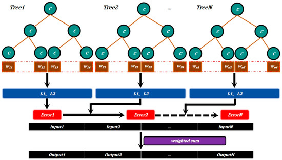
Figure 6. Extreme gradient-enhanced structure.

2.4.3. LSTM Model

A long short-term memory (LSTM) model can be applied to fit and predict time-series data. The LSTM is an improved version of the recurrent neural network (RNN). It introduces specially designed memory cells and gating mechanisms to deal with the long-term dependency problem, which traditional RNNs cannot effectively handle [26]. Traditional RNNs find it difficult to retain information over a long time, while the LSTM, through its unique design, can retain long-term information and suppress irrelevant information, making it particularly suitable for processing data with time-dependent characteristics. Compared with ordinary RNNs, LSTMs model long-term dependencies more accurately, giving them a significant advantage in processing complex time-series data.

The core of the LSTM network lies in its three gate mechanisms; namely, the input gate, the forget gate, and the output gate. These gates control how information flows in the memory cell [27]. Through the forget gate, the LSTM can selectively discard useless information from the past, and through the input gate, it can introduce new information to update the cell state. The output gate determines which parts of the cell state will affect the output at the current moment. Through the synergy of these gates, LSTM can dynamically adjust the content of memory cells, ensuring that the model has greater flexibility and accuracy in capturing long-term and short-term dependencies.

Specifically, when processing time-series data, LSTM calculates the input sequence of each time step through its layers of units in sequence. Unlike the simple hidden-state update of an ordinary RNN, LSTM adds a forget gate to each unit and refines the role of the input gate and output gate such that each unit can more reasonably choose which information should be retained, updated, or output. This mechanism greatly enhances the performance of the LSTM model in terms of long-term dependencies. As such, LSTMs have been widely used for a variety of tasks, including time-series prediction and natural language processing. The specific calculation process in each unit is as follows:

$$\begin{array}{c}{i}_t=\sigma (W_i\cdot [h_{t-1},x_t\left]\right)\end{array}$$

(9)

$$\begin{array}{c}{f}_t=\sigma (W_f\cdot [h_{t-1},x_t\left]\right)\end{array}$$

(10)

$$\begin{array}{c}{g}_t=\sigma (W_g\cdot [h_{t-1},x_t\left]\right)\end{array}$$

(11)

$$\begin{array}{c}{o}_t=\sigma (W_o\cdot [h_{t-1},x_t\left]\right)\end{array}$$

(12)

$$\begin{array}{c}{c}_t=f_t\odot c_{t-1}+i_t\odot g_t\end{array}$$

(13)

$$\begin{array}{c}{h}_t=o_t\odot {tanh(c}_t)\end{array}$$

(14)

In this study, the core structure of the long short-term memory network (LSTM) includes the hidden state $h_t$, the cell state $c_t$, the input $x_t$, the hidden state $h_{t-1}$ at the previous moment, and a series of gate units. Specifically, $h_t$ represents the hidden state at time $t$, $c_t$ represents the cell state at time $t$, and $x_t$ is the input at time $t$. The hidden state $h_{t-1}$ at the previous moment is the hidden state at time $t-1$ or the initial hidden state at time $t$= 0. In addition, the LSTM unit contains four key gate units: input gate it, forget gate ft, cell gate $g_t$, and output gate $o_t$. The function of these gates is to control the flow and update of information in the network through different mechanisms. $\sigma$ represents the Sigmoid function, and the symbol $\odot$ represents the Hadamard product, which is the operation of multiplying each element of the matrix one by one [28]. In traditional recurrent neural networks (RNNs), the output depends only on a linear combination of the current input and the hidden state of the previous moment. Therefore, when processing long time-series, the model will face the problem of “long-term dependency” and find it difficult to remember long-distance context information. By introducing a gate mechanism in the LSTM, the network can more precisely select information at each time step, deciding which information needs to be retained and which can be forgotten, thereby effectively alleviating the memory loss problem of traditional RNNs when processing long sequences. Specifically, the forget gate $f_t$ is responsible for determining which past information needs to be forgotten, while the input gate determines the contribution of the current input to updating the cell state, the cell gate $g_t$ controls the content of the cell state update, and, finally, the output gate $o_t$ determines which information will be used for the output.

It is precisely due to these refined control mechanisms that the LSTM network can flexibly manage the dependencies between long-term and short-term information, allowing it to perform well in processing time-series data. At each time step, the LSTM will comprehensively determine how to update the internal state of the model based on the current input and the hidden state and cell state of the previous moment, ensuring that important information is retained for a long time and irrelevant information is forgotten [29]. In this way, the LSTM network can deal with complex time-series problems more effectively.

With the evolution of models and the development of big data analysis needs, LSTM has become one of the mainstream methods for processing time-series data, and has been shown to perform well in various practical tasks, such as time-series prediction, natural language processing, and speech recognition. In this study, the LSTM network is also a key component, as its powerful modeling capabilities are used to handle the fitting and prediction of time-series data, effectively improving the model’s fitting and prediction performance. The structure of the long-term and short-term memory model is shown in Figure 7.

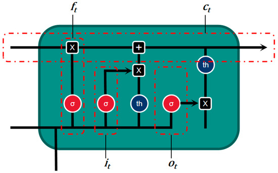
Figure 7. Unit structure diagram of a long short-term memory neural network.

3. Results

3.1. Correlation Analysis Results

This study uses the daily average PM_2.5 concentration at the monitoring sites as the dependent variable, and other site statistical variables after spatio-temporal matching are used as independent variables for Spearman correlation analysis. The analysis results show that PM_2.5 concentration is significantly correlated with AOD, temperature at 2 m above the ground, meridional wind speed and zonal wind speed at 10 m above the ground, boundary layer height, near-ground relative humidity, atmospheric pressure, population density, urban land, other construction land, and county roads, at least at the 0.01 level. Therefore, this study selected the above variables that passed the correlation test as independent variables to enter into the model.

3.2. Inversion Results Based on the XGBoost Model and LSTM Model

This study compared and analyzed the results of a PM_2.5 concentration simulation using the two models at each station through a density scatter plot.

PM_2.5 used in this study The daily station observation data covers 365 days from 1 January to 31 December 2023, and the original sample size is 23,696. In order to ensure the robustness of the model evaluation, the training set (70%, 16,587 items) and the test set (30%, 7109 items) were divided by random sampling according to the ratio of 7:3.

The analysis results of characteristic importance of xgboost model for various variables are shown in Figure 8 and Figure 9.

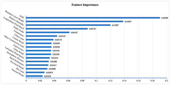
Figure 8. Characteristic weights of various variables.

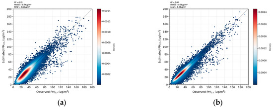
Figure 9. Density scatter plot of estimated and measured values for the XGBoost and LSTM models: (a) XGBoost; (b) LSTM.

This study compared and analyzed the results of a PM_2.5 concentration simulation using the two models at each station through a density scatter plot. The horizontal and vertical axes of the scatter plot represent the observed and simulated values of near-ground PM_2.5, respectively. At the same time, a 1:1 reference line (dashed line) is added to the figure to allow the model performance to be more intuitively evaluated. The color of the data points changes from blue to red according to the density, which clearly shows the density of the data distribution. In terms of model evaluation, the LSTM model shows a high coefficient of determination (R² = 0.88), which indicates that it can explain 88% of the variance of the target variable, has a good ability to capture the fluctuations of the actual observed values, and has a significant fitting effect. In contrast, the R² value of the XGBoost model is 0.75, which is slightly inferior. The root mean square error (RMSE), as a key indicator for measuring the prediction accuracy of the model, reflects the average deviation between the predicted value and the observed value. The RMSE of the LSTM model on the test set is 9.38 $\mathsf{\mu }\mathrm{g}/{\mathrm{m}}^3$, while the RMSE of the XGBoost model is 9.64 μg/m³, which shows that the average prediction error of the LSTM model is smaller. The mean absolute error (MAE) is also used to evaluate the prediction error of the model. The MAE of the LSTM model is 6.48 μg/m³, while the MAE of the XGBoost model is 6.82 μg/m³, which further confirms the advantage of the LSTM model in prediction accuracy. Combining the three indicators of R², RMSE, and MAE, the LSTM model is shown to be superior to the XGBoost model in terms of both goodness of fit and prediction performance, showing stronger generalization ability. In addition, although both models have a certain degree of underestimation, the degree of underestimation of the LSTM model is relatively mild. Overall, the LSTM model has superior performance in simulating the near-ground PM_2.5 concentration in the Yangtze River Delta urban agglomeration.

The area covered by this study was carefully divided into 27,333 3 × 3 km² longitude and latitude grid cells. The LSTM model and the XGBoost model simulated the near-surface PM_2.5 concentration for 365 days in 2023 and produced a total of 2,702,773 sets of data. By averaging the daily simulated data, this study successfully derived the daily average simulated value (estimated value) of the near-surface PM_2.5 concentration in the Yangtze River Delta urban agglomeration in 2023, and the data series are presented in the form of a line graph. At the same time, in order to achieve an intuitive comparison with the measured data, this study also shows the daily average station-observed values (observed value) of the near-surface PM_2.5 concentration in the form of a line graph.

It can be clearly seen from the Figure 10 that, in the Yangtze River Delta urban agglomeration, the daily average simulated value of the near-surface PM_2.5 concentration shows a high degree of consistency with the measured value and the two curves show an obvious trend of synchronous fluctuation. However, in some local periods, there is still a slight deviation between the simulated and measured values, which can mainly be attributed to the inherent limitations of the machine learning model itself. It is worth noting that in the overall comparison, the simulation value of the LSTM model is better than that of the XGBoost model in terms of the degree of fit of the data points, which strongly proves the advantage of the LSTM model in prediction accuracy.

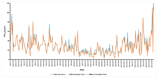
Figure 10. Time-series diagram of the daily average estimated PM_2.5 concentration and the daily average site observation value of PM_2.5 concentration.

Further analysis of the dynamic changes in the daily average data in 2023 shows that the near-ground PM_2.5 concentration reached its annual peak on 28 December, followed by a slight decline, and formed a second peak on 5 January. After February, the concentration value showed a steady downward trend and reached the lowest point of the year in July. From the overall annual perspective, the PM_2.5 concentration in winter is significantly higher than that in summer. This finding is of great significance for grasping the timing for the prevention and control of PM_2.5 pollution. The PM_2.5 concentration inversion map of the Yangtze River Delta urban agglomeration at quarterly time points is shown in Figure 11.

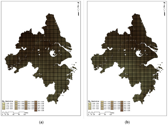
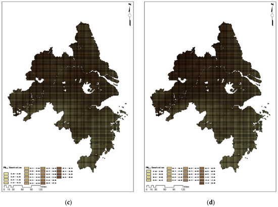
Figure 11. Retrieval results of PM_2.5 concentration in the Yangtze River Delta urban agglomeration at quarterly time points: (a) Retrieval results as of 1 March 2023; (b) Retrieval results as of 1 June 2023; (c) Retrieval results as of 1 September 2023; (d) Retrieval results as of 1 December 2023.

4. Conclusions

This study focused on the Yangtze River Delta region of China, relying on hourly PM_2.5 concentration data collected by 184 ground monitoring stations in 2023 and the sixth version of the MODIS aerosol optical thickness products from the Terra and Aqua satellites that has recently been released by NASA, including AOD data with a 3 km resolution inverted using the dark pixel algorithm (DT) and AOD data with a 10 km resolution inverted using the Deep Blue algorithm (DB). This study used the linear relationship between the AOD data of the two satellites, combined the advantages of the two data products, and performed linear interpolation to fill in the missing AOD data. On this basis, the fused AOD data were used as the main prediction factor, combined with the reanalysis meteorological data of the European Center for Medium-Range Weather Forecasts (ECMWF), population density, land use, and other auxiliary prediction factors. Spearman rank correlation analysis was performed to deeply explore the key factors affecting the changes in the spatiotemporal distribution of PM_2.5 concentrations. The results showed that PM_2.5 concentration is significantly correlated with AOD, temperature at 2 m above the ground, meridional and zonal wind speeds at 10 m above the ground, boundary layer height, near-ground relative humidity, atmospheric pressure, population density, urban land, other construction land, and county roads, all with a significance level of at least 0.01. Based on the above analysis, this study constructed an Extreme Gradient Boosting (XGBoost) model and a long short-term memory (LSTM) model for inversion of the PM_2.5 concentration. The results demonstrated that the LSTM model performs significantly better than the XGBoost model in terms of inversion accuracy. Specifically, the R² of the XGBoost model was 0.75, the root mean square error (RMSE) was 9.64 μg/m³, and the mean absolute error (MAE) was 6.82 μg/m³; while the R² of the LSTM model increased to 0.88, the RMSE was reduced to 9.37 μg/m³, and the MAE was reduced to 6.48 μg/m³. It can be seen that the LSTM model shows higher accuracy and feasibility in the context of PM_2.5 concentration estimation, and can be considered suitable for high-precision quantitative inversion work.

5. Limitations and Perspectives

In this study, linear interpolation and fusion methods were used to effectively fill in the areas where AOD data were missing, effectively increasing the amount of sample data for modeling. However, for areas where both Aqua and Terra AOD were missing and where there were no data for a long time, the aerosol optical thickness data required for the study could not be obtained through the AOD products provided by MODIS, resulting in an uneven spatial distribution and a discontinuous temporal distribution of the sample data. Therefore, the lack of sample data directly affected the fitting effect of the inversion models. Future research can consider combining aerosol data from multiple satellites to better address the problem of missing AOD data, improve data coverage, and achieve more accurate quantitative inversion.

The LSTM model used in this study can effectively solve the problem of spatiotemporal non-stationarity and showed a better fitting effect than the XGBoost model; however, the accuracy of the model is greatly affected by the amount of sample data. According to the experimental results, it can be found that the more sufficient the amount of sample data used for modeling, the more stable the trained model and the better the inversion result. However, due to various limitations, it is not guaranteed that sufficient sample data will be collected. Therefore, future research should try to improve and develop inversion models which remain suitable when only small amounts of sample data for the study of the dynamic spatiotemporal changes in PM_2.5 concentrations are available.

References

- Dennekamp, M.; Howarth, S.; Dick, C.A.J.; Cherrie, J.W.; Donaldson, K.; Seaton, A. Ultrafine particles and nitrogen oxides generated by gas and electric cooking. Occup. Environ. Med. 2001, 58, 511–516. [Google Scholar] [CrossRef] [PubMed]
- Happo, M.S.; Salonen, R.O.; Hälinen, A.I.; Jalava, P.I.; Pennanen, A.S.; Dormans, J.A.M.A.; Gerlofs-Nijland, M.E.; Cassee, F.R.; Kosma, V.-M.; Sillanpää, M.; et al. Inflammation and tissue damage in mouse lung by single and repeated dosing of urban air coarse and fine particles collected from six European cities. Inhal. Toxicol. 2010, 22, 402–416. [Google Scholar] [CrossRef]
- Duan, J.; Yu, Y.; Li, Y.; Jing, L.; Yang, M.; Wang, J.; Li, Y.; Zhou, X.; Miller, M.R.; Sun, Z. Comprehensive understanding of PM 2.5 on gene and microRNA expression patterns in zebrafish (Danio rerio) model. Sci. Total Environ. 2017, 586, 666–674. [Google Scholar] [CrossRef]
- Han, L.; Zhou, W.; Li, W.; Li, L. Impact of urbanization level on urban air quality: A case of fine particles (PM2. 5) in Chinese cities. Environ. Pollut. 2014, 194, 163–170. [Google Scholar] [CrossRef]
- Chen, C.Y.; Yin, X.B. Source, composition, formation and harm of PM2. 5 in haze. Univ. Chem 2014, 29, 1–6. [Google Scholar]
- Donner, L. Aerosols, Clouds, and Precipitation as Scale Interactions in the Climate System and Controls on Climate Change. In Proceedings of the APS March Meeting 2016, Baltimore, MD, USA, 14–18 March 2016; American Physical Society: College Park, MD, USA, 2016. [Google Scholar]
- Wu, R.; Dai, H.; Geng, Y.; Xie, Y.; Masui, T.; Liu, Z.; Qian, Y. Economic impacts from PM2. 5 pollution-related health effects: A case study in Shanghai. Environ. Sci. Technol. 2017, 51, 5035–5042. [Google Scholar] [CrossRef]
- Wang, J.; Wang, S.; Voorhees, A.S.; Zhao, B.; Jang, C.; Jiang, J.; Fu, J.S.; Ding, D.; Zhu, Y.; Hao, J. Assessment of short-term PM 2.5 -related mortality due to different emission sources in the Yangtze River Delta, China. Atmos. Environ. 2015, 123, 440–448. [Google Scholar] [CrossRef]
- Song, Y.; Hou, D.; Zhang, J.; O’Connor, D.; Li, G.; Gu, Q.; Li, S.; Liu, P. Environmental and socio-economic sustainability appraisal of contaminated land remediation strategies: A case study at a mega-site in China. Sci. Total Environ. 2018, 610, 391–401. [Google Scholar] [CrossRef] [PubMed]
- Zhang, Y.; Li, Z. Remote sensing of atmospheric fine particulate matter (PM2. 5) mass concentration near the ground from satellite observation. Remote Sens. Environ. 2015, 160, 252–262. [Google Scholar] [CrossRef]
- Van Donkelaar, A.; Martin, R.V.; Brauer, M.; Kahn, R.; Levy, R.; Verduzco, C.; Villeneuve, P.J. Global estimates of ambient fine particulate matter concentrations from satellite-based aerosol optical depth: Development and application. Environ. Health Perspect 2010, 118, 847–855. [Google Scholar] [CrossRef]
- Paciorek, C.J.; Yang, L. Limitations of remotely sensed aerosol as a spatial proxy for fine particulate matter. Environ. Health Perspect. 2009, 117, 904–909. [Google Scholar] [CrossRef]
- Kahn, R.; Banerjee, P.; McDonald, D. Sensitivity of multiangle imaging to natural mixtures of aerosols over ocean. J. Geophys. Res. Atmos. 2001, 106, 18219–18238. [Google Scholar] [CrossRef]
- Liu, B.; Tan, X.; Jin, Y.; Yu, W.; Li, C. Application of RR-XGBoost combined model in data calibration of micro air quality detector. Sci. Rep. 2021, 11, 15662. [Google Scholar] [CrossRef] [PubMed]
- Dhaliwal, S.S.; Nahid, A.-A.; Abbas, R. Effective intrusion detection system using XGBoost. Information 2018, 9, 149. [Google Scholar] [CrossRef]
- Meng, Y.; Yang, N.; Qian, Z.; Zhang, G. What makes an online review more helpful: An interpretation framework using XGBoost and SHAP values. J. Theor. Appl. Electron. Commer. Res. 2020, 16, 466–490. [Google Scholar] [CrossRef]
- Nielsen, D. Tree Boosting with XGBoost-Why Does XGBoost Win “Every” Machine Learning Competition. Master’s Thesis, NTNU, Trondheim, Norway, 2016. [Google Scholar]
- Shi, X.; Wong, Y.D.; Li, M.Z.; Palanisamy, C.; Chai, C. A feature learning approach based on XGBoost for driving assessment and risk prediction. Accid. Anal. Prev. 2019, 129, 170–179. [Google Scholar] [CrossRef]
- Wang, C.; Deng, C.; Wang, S. Imbalance-XGBoost: Leveraging weighted and focal losses for binary label-imbalanced classification with XGBoost. Pattern Recognit. Lett. 2020, 136, 190–197. [Google Scholar] [CrossRef]
- Lin, Y. A note on margin-based loss functions in classification. Stat. Probab. Lett. 2004, 68, 73–82. [Google Scholar] [CrossRef]
- Shahani, N.M.; Zheng, X.; Liu, C.; Hassan, F.U.; Li, P. Developing an XGBoost regression model for predicting young’s modulus of intact sedimentary rocks for the stability of surface and subsurface structures. Front. Earth Sci. 2021, 9, 761990. [Google Scholar] [CrossRef]
- Asselman, A.; Khaldi, M.; Aammou, S. Enhancing the prediction of student performance based on the machine learning XGBoost algorithm. Interact. Learn. Environ. 2023, 31, 3360–3379. [Google Scholar] [CrossRef]
- Song, K.; Yan, F.; Ding, T.; Gao, L.; Lu, S. A steel property optimization model based on the XGBoost algorithm and improved PSO. Comput. Mater. Sci. 2020, 174, 109472. [Google Scholar] [CrossRef]
- Zhang, D.; Gong, Y. The comparison of LightGBM and XGBoost coupling factor analysis and prediagnosis of acute liver failure. IEEE Access 2020, 8, 220990–221003. [Google Scholar] [CrossRef]
- Zhang, P.; Jia, Y.; Shang, Y. Research and application of XGBoost in imbalanced data. Int. J. Distrib. Sens. Netw. 2022, 18, 15501329221106935. [Google Scholar] [CrossRef]
- Yu, Y.; Si, X.; Hu, C.; Zhang, J. A review of recurrent neural networks: LSTM cells and network architectures. Neural Comput. 2019, 31, 1235–1270. [Google Scholar] [CrossRef] [PubMed]
- Van Houdt, G.; Mosquera, C.; Nápoles, G. A review on the long short-term memory model. Artif. Intell. Rev. 2020, 53, 5929–5955. [Google Scholar] [CrossRef]
- Sherstinsky, A. Fundamentals of recurrent neural network (RNN) and long short-term memory (LSTM) network. Phys. D Nonlinear Phenom. 2020, 404, 132306. [Google Scholar] [CrossRef]
- Lindemann, B.; Müller, T.; Vietz, H.; Jazdi, N.; Weyrich, M. A survey on long short-term memory networks for time series prediction. Procedia Cirp 2021, 99, 650–655. [Google Scholar] [CrossRef]
Disclaimer/Publisher’s Note: The statements, opinions and data contained in all publications are solely those of the individual author(s) and contributor(s) and not of MDPI and/or the editor(s). MDPI and/or the editor(s) disclaim responsibility for any injury to people or property resulting from any ideas, methods, instructions or products referred to in the content. |
© 2025 by the authors. Licensee MDPI, Basel, Switzerland. This article is an open access article distributed under the terms and conditions of the Creative Commons Attribution (CC BY) license.