Article

Assessing the Impact of Sensor Height on the Representativeness of Temperature-Monitoring Sites in a Dense Midrise Urban Development Using PALM-4U

by
Florian Steigerwald
,
Astrid Eichhorn-Müller
,
Heike Schau-Noppel
and
Meinolf Kossmann
*
Deutscher Wetterdienst, P.O. Box 10 04 65, 63004 Offenbach, Germany
*
Author to whom correspondence should be addressed.
Atmosphere 2025, 16(9), 1035; https://doi.org/10.3390/atmos16091035
Submission received: 25 July 2025 / Revised: 25 August 2025 / Accepted: 29 August 2025 / Published: 31 August 2025
(This article belongs to the Special Issue Recent Advances in Urban Climate)

Abstract

In the context of ongoing global warming and urbanization, the need for reliable temperature monitoring in urban areas is increasing. Such monitoring serves multiple purposes, including assessing urban heat island (UHI) intensity, evaluating climate adaptation strategies, and supporting heat warning systems. This study utilizes high-resolution urban climate simulations with PALM-4U for calm, clear-sky summer weather conditions and an idealized model domain. The domain represents a dense midrise urban district in Dresden Neustadt, eastern Germany. Areas with air temperatures representative of the pedestrian level within the urban development are determined using a methodology based on a 24-h temporal moving representativity range defined by the temperature’s spatial median value and standard deviation. The method is extended by an evaluation of different temperature sensor heights, addressing practical considerations such as vandalism prevention and space availability. The results highlight the feasibility of representative pedestrian-level air temperature monitoring in densely built-up urban areas, particularly at elevated sensor heights between 2.5 and 6.5 m. It is found that higher sensor heights increase the area suitable for representative pedestrian-level temperature monitoring by up to about 50%. The sensitivity of the results to variations in wind speed and building height is also examined, demonstrating the robustness of the proposed method in clear, calm summer weather conditions.

Graphical Abstract

1. Introduction

Due to ongoing global warming, heat stress is becoming a growing issue in most regions of the world. The urban heat island effect [1], together with the growing urbanization, further exacerbates this issue. Today, more than 56% of the global population lives in cities [2]. Higher temperatures affect quality of life, health risks, housing demands, irrigation needs, and energy consumption, making adaptation strategies necessary. Therefore, the number of studies on the urban heat island has increased during the last decades [3]. and the demand for temperature monitoring in urban areas is rising. Since the 19th century, temperature monitoring has improved both technologically and methodologically, with a high level of global standardization driven by the World Meteorological Organization (WMO) [4]. Here, the focus has been on ensuring that measurements are representative of as large an area as possible. As a consequence, most weather and climate stations are situated in rural and comparatively homogenous areas. This challenge is most pronounced in inner-city districts, where building density is highest.
Recently, more and more municipalities and research projects use meteorological stations or low-cost sensing in urban environments, with objectives such as accurately monitoring the amplitude of warming in city quarters [5,6,7], analyzing the impact of climate adaptation measures [8], setting up an urban heat warning framework [9], or energy planning. Another common objective is the validation of numerical models or results from remote sensing. For all these objectives, the quality and representativity of the data, which are determined by station location, are crucial. However, the search for a suitable monitoring site in urban areas, especially in densely built-up city centers, is challenging. Complex urban morphology affecting radiation balance, wind fields, and surface variability (grass, asphalt, stone, pavement, etc.) creates strong horizontal temperature inhomogeneities, even within seemingly uniform areas. Additionally, aspects like ownership, traffic of cars and pedestrians, or monument protection may strongly limit the space available for measuring sites. Some guidance for the selection of a monitoring site in urban areas is given by the WMO’s “Initial Guidance to Obtain Representative Meteorological Observations at Urban Sites” [10], which provides broad guidance on monitoring temperatures in urban areas, supplemented by the “Guidance on Measuring, Modelling and Monitoring the Canopy Layer Urban Heat Island (CL-UHI)” [11]. However, both guides lack the clear instructions and standardization known from the synoptic scale monitoring guide [4]. Despite the increasing number of urban measurement studies, to our knowledge, there are no publications that investigate the representativeness of meteorological measurement sites within densely built-up areas.
Therefore, the general aim of our study was to find criteria that might increase the probability that a chosen measuring site is actually representative of the surrounding district. In a first step, we limit our study to near-surface air temperature. Secondly, our study focuses on calm and clear weather conditions, since temperature inhomogeneities are usually the strongest during these conditions. To capture the strong horizontal, vertical, and temporal variations in the temperature field within an urban setting, measurements would require setting up a very dense three-dimensional network comprising different streets and backyards, which is simply not feasible. In contrast, three-dimensional fields of air temperature or other parameters can be easily produced with a numerical urban climate model with very high resolution. For our study, we used the urban microscale model PALM-4U [12] with a horizontal and vertical grid spacing of 1 m (see Section 2) to locate representative monitoring sites in the dense urban canopy. The point-to-volume representativity method developed by Nappo [13], using model-based calculation of station representativity, is widely used in air pollution monitoring on the regional scale [14,15] and on the urban scale [16,17], but it has not yet been adapted to temperature sensing in urban environments. A key advance of this study is the extension of the method into the third dimension (z-direction), as in urban areas the horizontal variation of near surface air temperature may exceed the vertical variation. In this way, it is possible to analyze whether monitoring air temperature at greater sensor heights will decrease or increase the probability of measuring at a representative location. The proposed method is tested for an urban quarter of Local Climate Zone (LCZ) 2 “dense midrise” [18], which is typical for city centers in Germany.

2. Methodology

2.1. Model Description

The basis of this study is the Large Eddy Simulation (LES) Model PALM-4U (short for PALM for urban applications), version 23.10. PALM-4U allows the simulation of the urban atmosphere at a building-resolving resolution for model domain sizes ranging from quarters to entire cities [19,20,21,22]. PALM solves the incompressible, non-hydrostatic, filtered Navier–Stokes equations using the Boussinesq approximation for wind and scalar variables. At the sub-grid scale, a 1.5-order closure model based on the Deardorff kinetic energy scheme is used to parameterize the terms emerging from filtering [23]. Advection is discretized with a fifth-order scheme and time integration with a third-order Runge–Kutta scheme [24].
For the given urban application, the land surface model [25], the urban surface model [26], a radiation model, the plant canopy model, and the biometeorology module are added to the PALM core [27]. Further information on PALM is provided by Maronga et al. [11]. The suitability of PALM-4U for the presented study has been demonstrated by many earlier studies [19,26,28,29,30,31,32].

2.2. Case Description

The model simulations use the basic meteorological settings developed during the project “Urban Climate Under Change [UC]2, phase 2 module C”, for an idealized calm, clear-sky summer condition [30]. Cyclic boundary conditions are used in order to represent an idealized neighborhood to the area of interest with the same climatic properties. The 3D simulation is initialized with a vertical temperature profile that is nearly neutral in the lowest 20 m, followed by a strong inversion between 20 m and 50 m above ground and a nearly neutral stratification aloft.
For this study, different model setups are tested for their impact on representativeness, but all share the same basic settings: the model domain with the highest spatial resolution used for the presented analysis, here further referred to as the child domain, is a 400 m × 400 m × 100 m grid with a cell width and height of 1 m. This very high resolution allows us to capture the complex airflow and radiation interaction within the dense urban canopy layer (UCL) (Figure 1). The child domain is nested one way into a 2 km × 2 km parent domain with a 5 m grid spacing in all dimensions. One-way nesting describes the one-directional data transfer, i.e., the meteorological forcing, from the parent domain to the child domain, but not vice versa. A rule of thumb for LES modeling suggests that the horizontal domain width for complete turbulence development should be at least as wide as the atmospheric boundary layer (ABL) height, which can reach up to 2000 m [33]. The ABL is referred to as the urban boundary layer (UBL) when it is strongly influenced by buildings [1]. This means that the top of the parent domain must extend above 3000 m. This is achieved by stretching the height of the grid cells gradually from 5 m to 50 m by a stretch factor of 1.08 starting at 200 m above the ground. This results in a 3311 m high parent domain with 400 × 400 × 120 grid cells, which should meet the turbulence criteria. The parent domain itself is constructed by horizontally replicating the child domain to avoid disturbances of the data by other neighboring land use classes with different climatic characteristics. The clones of the child domain are separated by a 12 m wide gap sealed with pavement type 1, “asphalt/concrete mix”, serving as an artificial street canyon to prevent airflow trapping. The simulations of the reference run start on 27 July at 00:00 CEST (UTC+02), simulating idealized, calm, clear-sky, summer weather conditions with a geostrophic wind of 1 m/s blowing from the west. At this day of the year, the sun angle corresponds to the average sun angle for the summer months June, July, and August. The settings for geostrophic wind speed are varied to investigate the sensitivity of the proposed method to changes in meteorological conditions. The simulation time is uniformly set to 48 h, where the first 24 h are considered as spin-up time and are therefore not included in the evaluation. The model output is averaged over 10 min intervals.

2.3. Model Area and Static Driver

The distribution of buildings, streets, backyards, and pavement types in the child domain is loosely based on a section of Dresden Neustadt (Germany), centered around the junction of Förstereistraße and Jordanstraße (Figure 1). This area was chosen for its relatively homogeneous structure, characteristic of LCZ 2 “dense midrise” [18], a very common local climate zone in the dense urban centers of central Europe [34].
The lower-left corner of the child domain is located at latitude 51.66520° north and longitude 13.74728° east, corresponding to an ETRS89/UTM zone 33N origin at x: 412,224 m and y: 5,657,969 m. The parent domain was constructed by horizontally replicating the child domain (see Section 2.2), with its origin at x: 411,424 m and y: 5,657,169 m ETRS89/UTM zone 33N (Figure 1). Building data were taken from OpenStreetMap. Since only a small number of building polygons included height information, the remaining buildings were assigned a default height of 20 m. Additional simulations were performed using building heights of 17 m and 14 m to assess their impact on representativity (see Section 3.4). All buildings were classified as residential buildings constructed between 1950 and 2000. Street data from OpenStreetMap were represented as lines with the number of lanes, but without lane widths. A width of 4 m per lane was assumed for all streets (Figure 1).

2.4. Calculation of Spatial and Temporal Representativity

A key question in identifying representative monitoring sites is how “representativity” is defined and measured. For our study, we use the method proposed by Nappo [13], who states the following definition: “Representativeness is the extent to which a set of measurements taken in a space-time domain reflects the actual conditions in the same or different space-time domain taken on a scale appropriate for a specific application”. The representativity definition developed by Nappo [13] is used in urban climate sciences primarily in the field of air quality measurements and particle dispersion on the regional scale [14,15], but it has proven its applicability even in the complex urban climate [16,17]. In this study, representativeness of the measurements at site (xm, ym, zm) for the temperature in the study area of interest at height zr is as follows:
RI x m , y m , z m =   Pr t = 0 144 T x m , y m , z m , t x ˜ T z r , t   σ T z r , t
   RI x , y 90 %     Representative RI x , y < 90 %     Not   representative
The air temperature T(xm,ym,zm,t) at the measurement coordinates xm, ym, with the measurement height zm is representative of T(zr,t) in the model domain at z = 1.5 m (zr) and at the given time t, if the absolute difference between T(xm,ym,zm,t) and the median of T(zr,t), x ˜ T (zr,t), of all non-building cells at zr is less than or equal to the standard deviation of T(zr,t), σT(zr,t), of all non-building cells at zr. The probability (Pr) that T(xm,ym,zm,t) lies within these bounds over a diurnal cycle is called the Representativity Index, RI(xm,ym, zm). If a cell’s RI is ≥90%, the cell is considered representative. This threshold of 90% is suggested by Nappo [13] and is adopted by this study. The evaluated diurnal cycle begins at 22:00 UTC (00:00 CEST) and ends 24 h later at 22:00 UTC, with a 10-min output interval (144 timesteps). In the work by Nappo [13], the vertical dimension is not included. We add the z-dimension to evaluate the representativity at different measurement heights.

2.5. Sensitivity Simulation Settings

In order to evaluate the transferability of the representativity method to other meteorological situations and different building parameters, a basic sensitivity analysis is carried out. The main focus is the impact of wind speed as well as of building heights. In the Baseline simulation, the large-scale windspeed is set to 1 m/s, and the median building height is 20 m (Table 1). In the sensitivity runs, large-scale geostrophic wind speed is increased to 2 m/s and 3 m/s, and building height is reduced to 17 m and 14 m.

3. Results and Discussion

The analysis of this study is based on the temperature distribution in the model domain over the time interval between 22:00 UTC on July 27th and 22:00 UTC on July 28th. The terms sunrise and sunset will continue to refer to the times when sunlight enters or leaves the street canyons at ground level, in distinction from the actual sunrise or sunset, which occur on the natural horizon at different times.

3.1. General Simulation Results

The representativeness of monitoring sites depends mainly on the spatial temperature variability in the area of interest, which is a direct consequence of inhomogeneous energy fluxes. Buildings, trees, and different surface properties generate these inhomogeneities due to shading, redirecting airflow, or albedo variations in the pavements and facades. As a rule of thumb, the higher the complexity in the area of interest, the harder it is to locate a representative monitoring site.
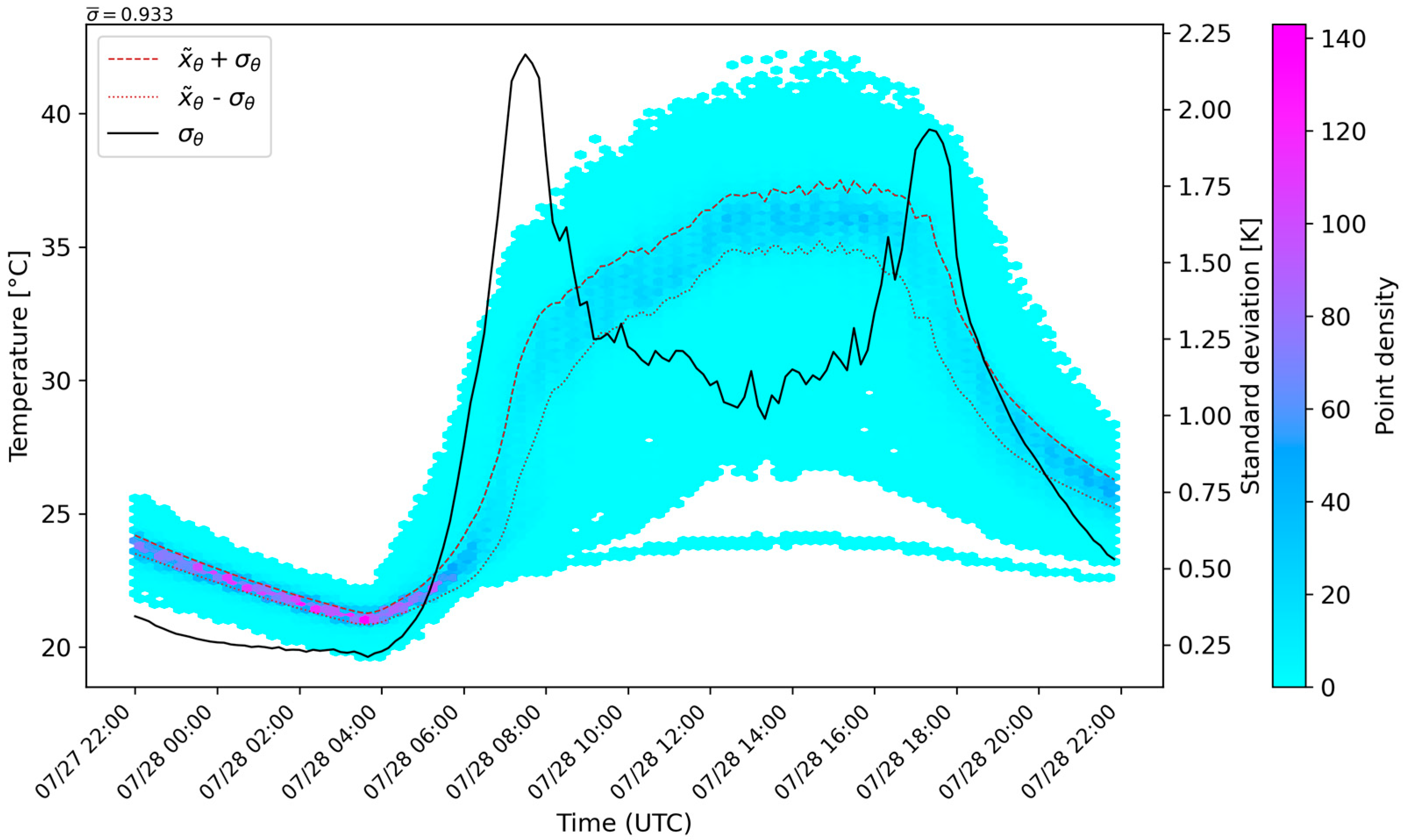
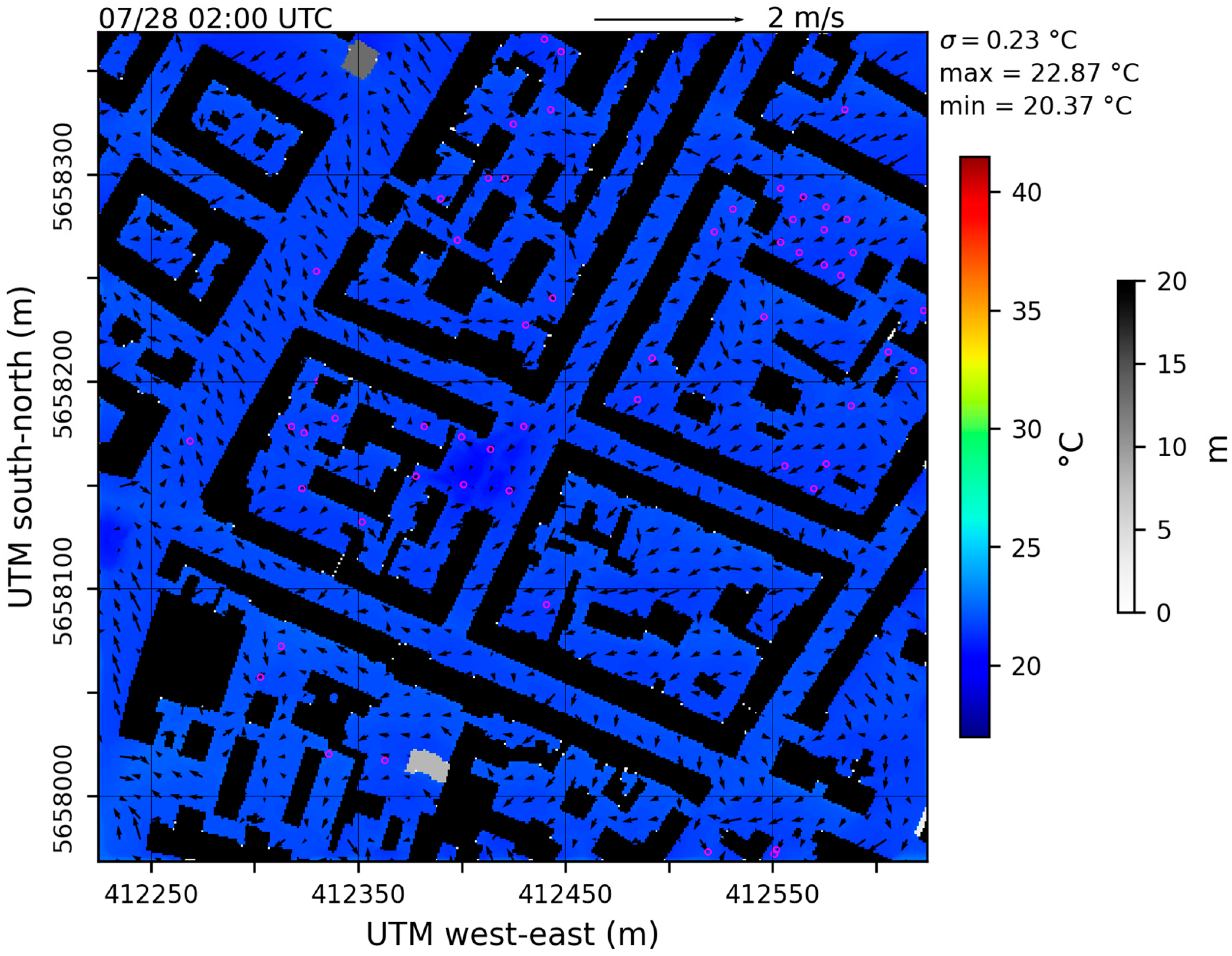
The diurnal cycle of temperature at pedestrian level (1.5 m) starting at 22:00 UTC (00:00 CEST) shows typical cooling during nighttime down to an area median minimum of 22 °C with a low standard deviation of 0.25 K (Figure 2). During the night, shortwave radiation—which drives spatial temperature variability during daytime—is zero, and surface energy balance terms show lower magnitudes. This results in a relatively uniform nocturnal air temperature distribution at pedestrian level (Figure 3).
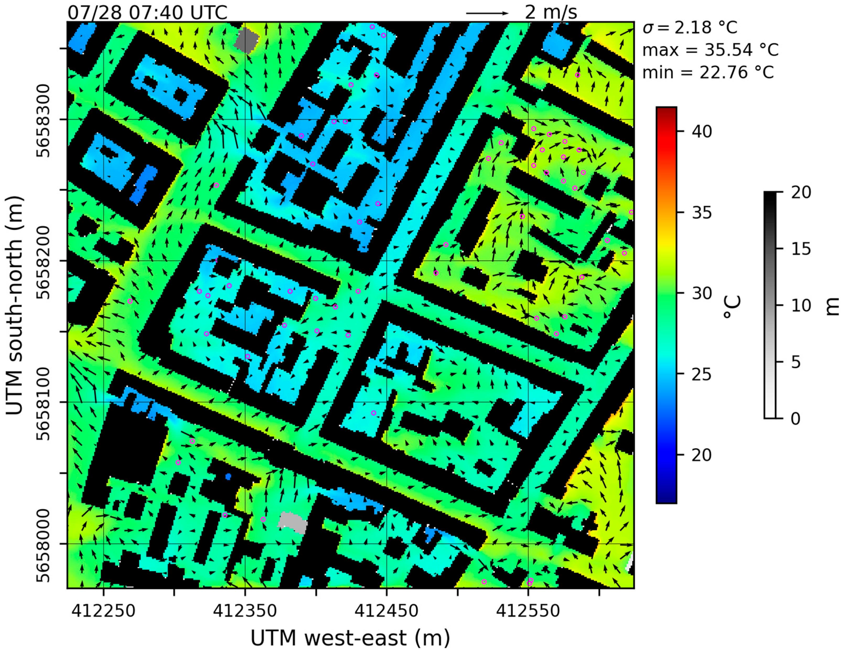
In the morning, as the first rays of sun warm roofs, favorably oriented walls, and other surfaces, the resulting inhomogeneous energy input sharply increases spatial temperature variability. The standard deviation in the model area rises to 2.18 K at 07:40 UTC (09:40 CEST) (Figure 2 and Figure 4). Shaded street canyon floors in the dense inner building blocks remain relatively cool, while more open areas already receive solar radiation. The temperature median at 1.5 m reaches its maximum of 36 °C at around 15:00 UTC (17:00 CEST), with local temperature peaks above 41 °C, while the standard deviation fluctuates around 1.2 K. As the sun angle decreases in the afternoon, the standard deviation rises, driven by the expansion of shaded ground surfaces. When the sun slowly sets in the afternoon, the same effect occurs as during sunrise. While some areas are still heated by solar radiation, the radiation balance of shaded cells becomes negative, thus increasing the spatial temperature variability to a standard deviation of over 1.9 K. The diurnal cycle of spatial air temperature variability evident in Figure 2, Figure 3 and Figure 4 illustrates the complexity of the diurnal temperature distribution, which the representativity method needs to consider.

3.2. Spatial and Temporal Representativity

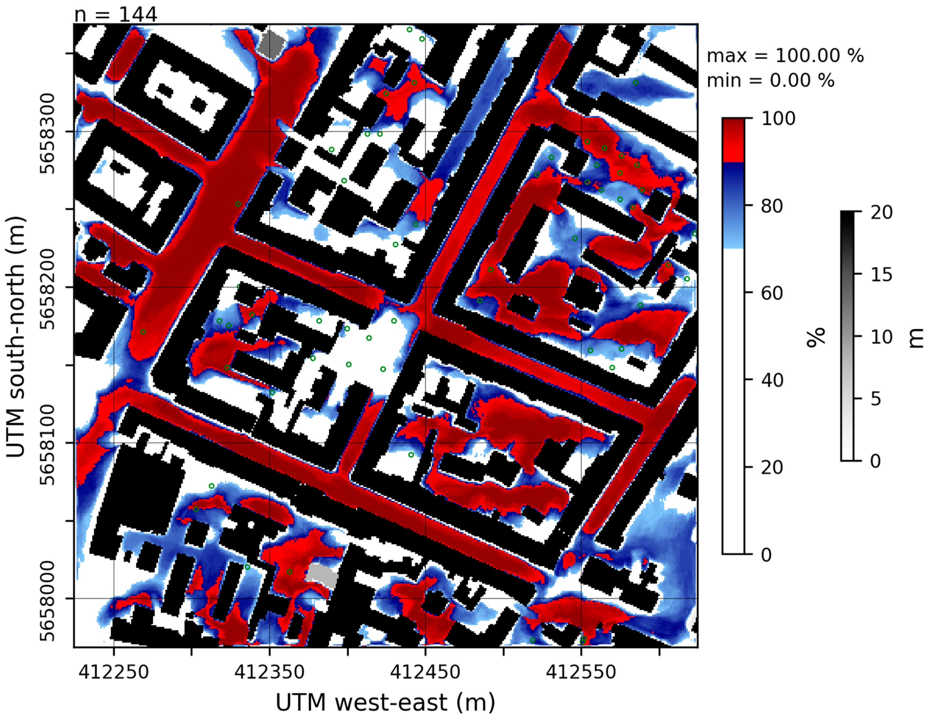
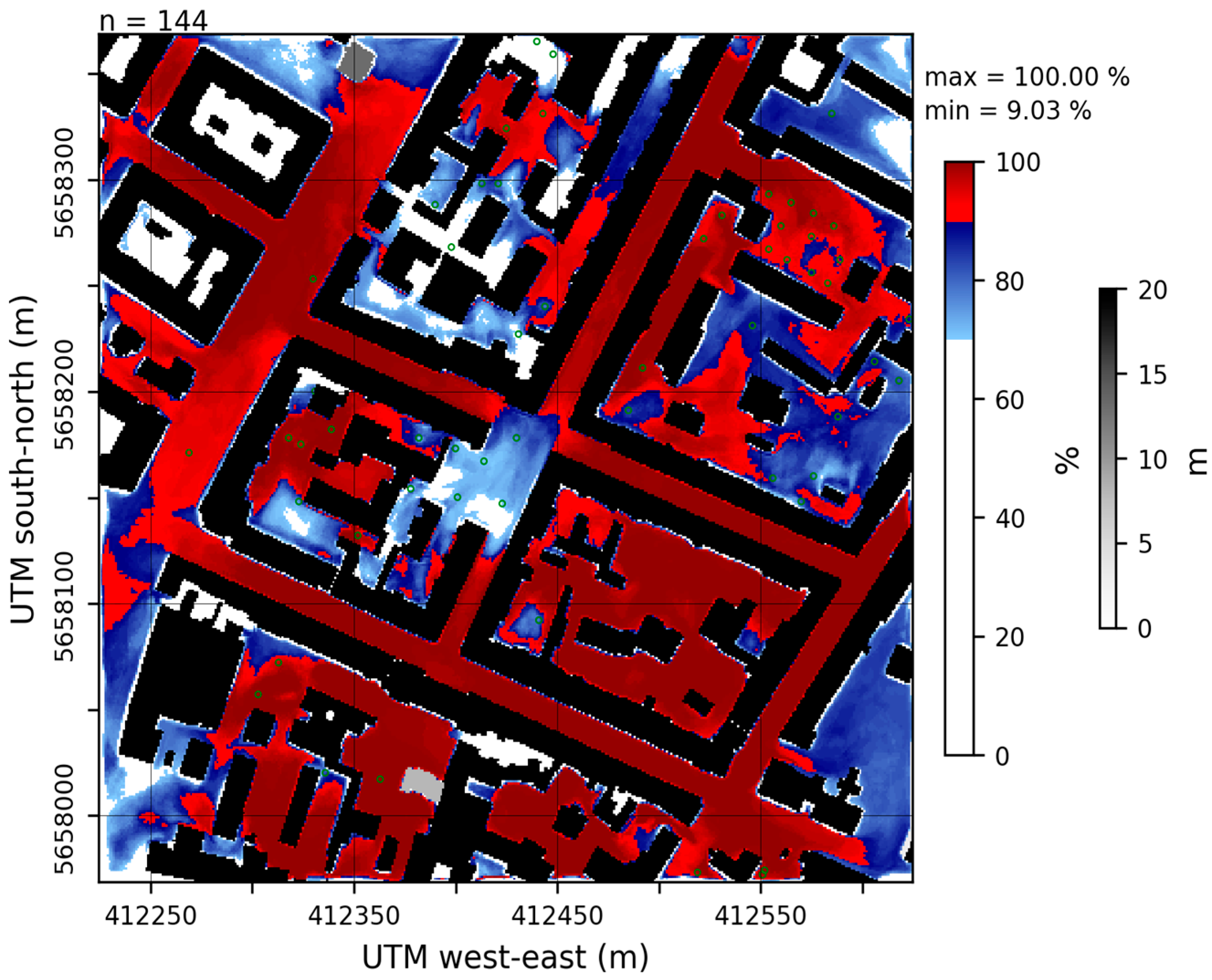
The RI at 1.5 m height for the child domain calculated from 07/27 22:00 UTC to 07/28 22:00 UTC is shown in Figure 5. Red shading indicates representative areas in which the algorithm, described in Section 2.4, yields RI ≥ 90%, i.e., temperature values are within the thresholds given by the temperature median ± σT 90% of the time. The areas of the highest representativity are located in the main street canyons and within medium dense building blocks (B5 and B8). Surfaces with a very low sky view factor, such as the northeastern part of B9 and the southern part of B2, tend to be not representative. The same applies to closed, chimney-like courtyards, such as B1 and B4. The air within these closed building structures is decoupled from the airflow aloft, which prevents effective mixing. It is also noteworthy that the representativeness of model cells in proximity to building walls not facing north also exhibit low representativeness. These walls are heated up by shortwave radiation over the day, creating an air layer in the adjacent model grid cells with temperatures frequently exceeding the median ± σT threshold for representativity during daytime.
There are non-meteorological conditions, such as land use, land ownership, or access to electric power, that can severely limit the availability of areas for meteorological measurements. Therefore, the areas that are excluded for meteorological reasons should not be too large. In our view, the method presented is a good compromise. However, in cases when a more stringent definition of the representativity is required, it is possible to include a multiplicative factor < 1 in the representativity equation, which reduces the representativity range. The representativity range could be reduced further to the point where only a few model cells with extremely high representativity remain. A similar effect would occur when changing the representativity threshold defined by Nappo [13] of 90%. An increased threshold would reduce the number of representative monitoring locations and vice versa. For example, in Figure 5, the 90% threshold considers all red areas representative; at 95%, only the dark red areas remain representative, whereas at 70%, both red and blue areas qualify. The 90% threshold represents a suitable middle ground, providing a reasonable area of potential representative monitoring while maintaining a high RI.

3.3. Influence of Simulated Measurement Height on Representativity

As many areas at pedestrian level with RI ≥ 90% are located within private building blocks or on streets, a conflict of use between the monitoring station and infrastructure demands will decrease the size of available areas. To address this, a flexible measurement height component is added to Nappo’s approach [13] to investigate the advantages and disadvantages of an increased measurement height, as suggested by Oke [10]. This approach is based on the assumption that the UCL exhibits near-neutral stratification throughout the day, a necessary condition to avoid potential measurement bias due to stratification in street canyons. As demonstrated by Nakamura and Oke [35], the presence of near-neutral stratification is characteristic of the UCL in street canyons.
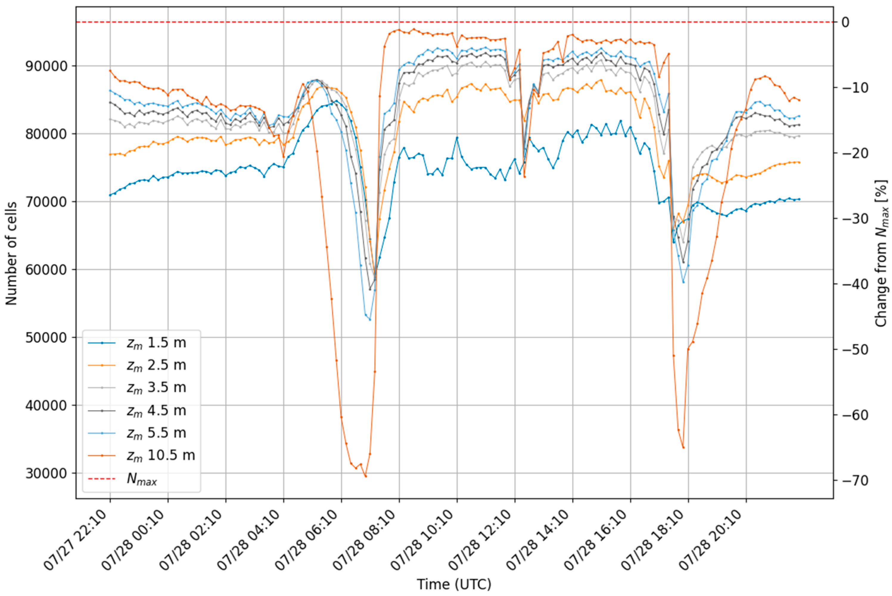
Analyzing the representativeness at different measuring heights (zm) (Figure 6) reveals two opposing effects. Most of the day, and especially during nighttime, the number of cells representative of air temperature at 1.5 m increases with elevated zm. However, at around 12 UTC, around sunset, and most pronounced around sunrise, the number of representative cells decreases significantly with increasing zm.
Monitoring temperature at higher altitudes can improve representativeness if the stratification within street canyons remains near neutral due to mixing in the UCL and the fact that, within a street canyon, heating or cooling occurs not only from the ground but also from the walls, i.e., the sides. Near-neutral stratification implies that temperature variation with height is small. At the same time, a larger distance from the ground allows for stronger horizontal mixing, and the influence of underlying hot surfaces (low albedo asphalt) or cool surfaces (tree-shaded short grass) is reduced. This means that an increased distance from the ground leads to a more homogenized view of the strong spatial temperature variability at the pedestrian level. This can be seen also in the diurnal cycle of the spatial standard deviation (σT) (see Section 3.4): As long as the stratification or height-induced measurement error is low, i.e., with a near-neutral stratification, the spatial standard deviation (σT) decreases with increasing height. This is not the case at sunset and sunrise, when shading leads to a high spatial variability of cooling or heating, not only from the ground but also from the walls and roofs. In contrast to the day or night situation, the stratification in the street canyon is now stable (see Section 3.4)), preventing vertical turbulent mixing and therefore extending the response time of air temperature at higher levels to surface cooling or heating. This stable stratification is the result of the vertical gradient in incoming shortwave radiation. The ground surfaces are shaded, but the building walls with an eastern (sunrise) and western (sunset) orientation as well as the building roofs are still or already illuminated. As the urban development in the model domain is very dense, the air still becomes heated in the upper part of the street canyons. The wind above the buildings also mixes warmer air from the still-illuminated rooftops into the upper street canyon, inducing a temperature increase in the z-direction within the UCL, i.e., stable stratification (see Section 3.4).
Another phase with lower numbers of representative grid cells at heights above 2.5 m occurs around high noon. Between approximately 12:00 UTC and 13:00 UTC, a destabilization of the temperature profiles in the street canyons leads to a significant temperature difference between elevated sensor heights above 1.5 m and at pedestrian level (1.5 m). Consequently, the representativeness of elevated sensor heights for the pedestrian level during this period is reduced (Figure 6 and Section 3.4).
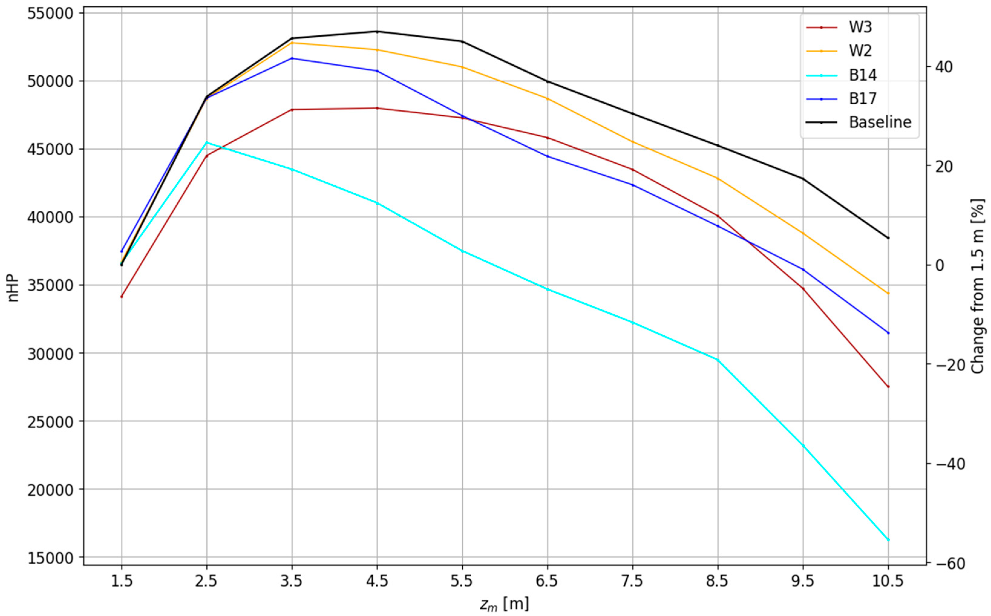
The balance between the turbulence-induced blending and the stratification-induced measurement errors results in an optimal measurement height between 2.5 and 6.5 m. At these heights, the number of cells representative of pedestrian-level air temperature is higher than at the pedestrian level itself (Figure 7, Baseline). This means that the choice for siting stations to measure temperatures that are representative of the pedestrian level is biggest at sensor heights between 2.5 and 6.5 m. The optimal measurement height zm suggested by the Baseline run is 4.5 m, where the number of representative cells is over 50% higher compared with the pedestrian level (Figure 7), resulting in the distribution of representative areas shown in Figure 8. The cells with an RI ≥ 90% cluster around areas of similar building density, which confirms the guidance of Oke [10], who suggests choosing an area with a spatial representative aspect ratio of building height and street width for locating temperature monitoring stations in urban environments. Areas with high building density and, consequently, comparatively low sky-view factors, such as B2 or the northwestern corner of B9, tend to have air temperatures that are unrepresentative of the model domain. Furthermore, areas with high sky-view factors such as the southeast or northwest of the child domain also show a low RI.
It is also noticeable that temperatures adjacent to non-northern-oriented building walls are not representative. This is for the same reason as previously described for RI at a height of 1.5 m. Figure 8 also shows the non-representativity of the green areas (Figure 1), which results from their stronger cooling at night compared with the sealed surfaces. With temperatures 1.5 m above the green areas being 0.6 K lower than the domain’s median, these model cells are outside the representativity range defined by σT of around 0.25 K before sunrise (Figure 1 and Figure 5). When surfaces between buildings are predominantly sealed, installing a temperature monitoring station in a green area leads to an underestimation of the temperatures in the urban quarter during the night and is therefore not recommended.

3.4. Sensitivity

To assess the sensitivity of the proposed representativity method to meteorological conditions on the one hand and to the street canyon aspect ratio on the other hand, a series of simulations was carried out. This paper focuses on the sensitivity of representativity to wind speed and building height.

3.4.1. Wind Speed Sensitivity

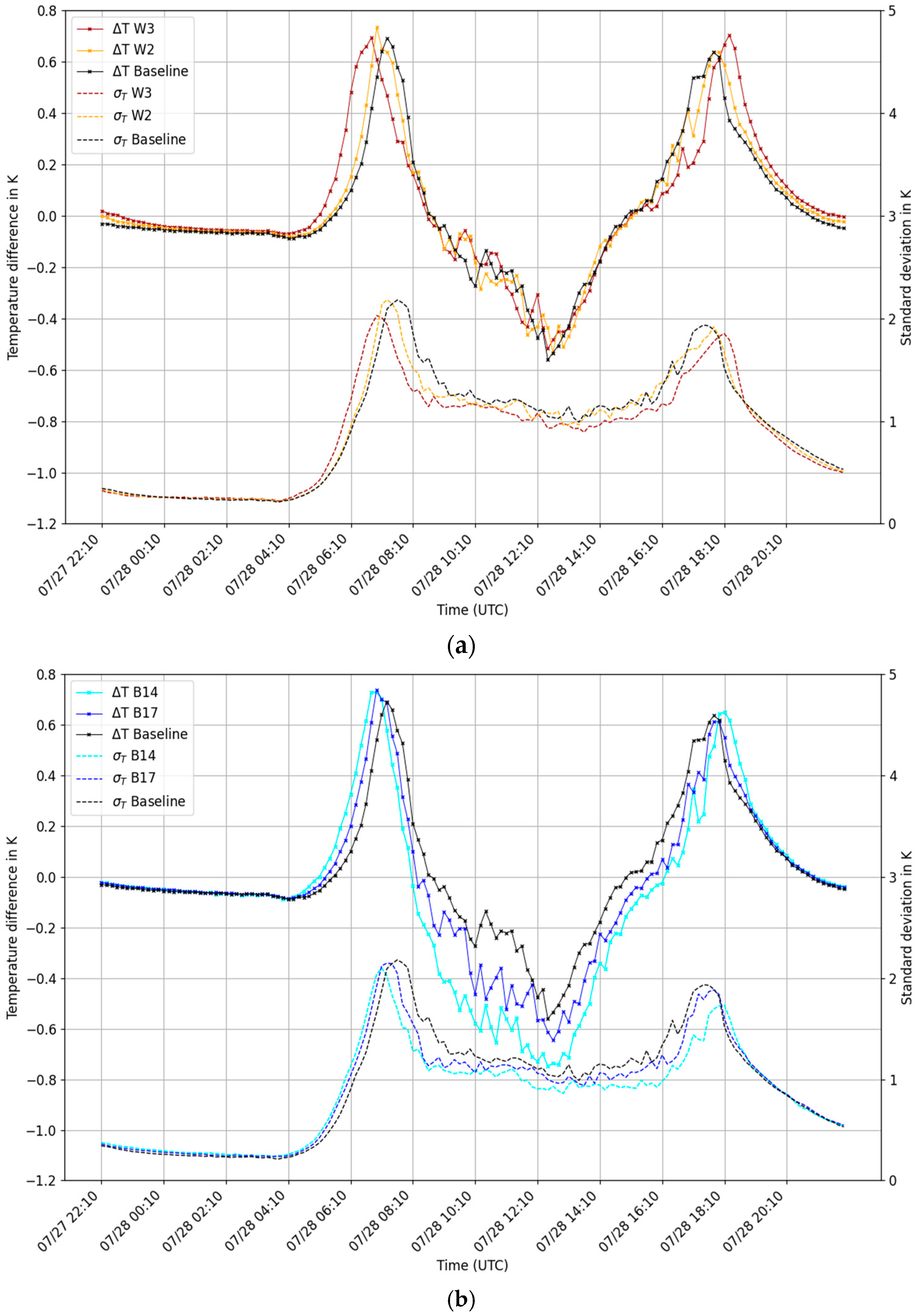
Wind speed magnitude in street canyons is a key factor in representativity analysis as stronger winds enhance turbulent mixing within the UCL, leading to a lower temperature standard deviation (Figure 9a). This lower spatial temperature variability reduces the representativity range defined by the temperature median ± σT. However, the magnitude of the simulated measurement error ΔT induced by stratification does not change significantly with higher wind speeds, as shown in Figure 9a. Only the timing of the sunset and sunrise temperature difference peaks shifts. At sunrise, the higher geostrophic wind speeds of 2 m/s and 3 m/s lead to stronger and earlier down-mixing of radiation-heated roof air into the street canyon. This results in an earlier peak (ΔT) with a magnitude comparable to that of the 1 m/s simulation. At sunset, stronger turbulent mixing delays the radiation-induced stabilization of thermal stratification in street canyons until the influence of heterogeneous energy input overpowers the counteracting turbulent mixing. For higher wind speeds, the narrower representativity range combined with a similar diurnal amplitude of the simulated measurement errors result in a lower number of representative cells at greater measurement heights compared with the Baseline simulation. Nevertheless, even under conditions with higher wind speeds, a sensor height of at least up to 9.5 m shows to be more effective than measuring air temperature at the pedestrian level (1.5 m) (Figure 7).

3.4.2. Building Height Sensitivity

Incoming shortwave radiation is a main driver of spatial temperature variability within the densely built-up urban quarter, as shown above. Therefore, the sensitivity of the results to building height is important to assess the generalizability of the methodology. For this purpose, three different median building heights were simulated: Baseline (20 m), B17 (17 m), and B14 (14 m).
The results reveal that lower building heights and therefore less shading reduce the diurnal amplitude of the spatial temperature standard deviation, especially in the B14 run (Figure 9b). On the other hand, decreasing building height causes the stable stratification (positive ΔT in Figure 9b) to persist longer after sunrise and to onset earlier at sunset. This shift of up to about 1 h in transition times between stable and unstable stratification occurs due to the timing of the first sunlight illuminating the ground floor of the street canyons. During daytime hours with strong insolation, the measurement error ΔT increases with decreasing building height. The stronger unstable stratification results from less shading and, therefore, higher shortwave energy input for lower building heights. The error ΔT reaches a maximum of −0.75 K around noon (run B14), which is of a magnitude similar to the maximum positive ΔT values at sunrise and sunset, but it must be evaluated against the representativity range at the corresponding time of the day, which depends on the standard deviation. At sunrise, σT peaks at 2.25 K (Figure 9) with a measurement error of around 1 K for zm = 4.5 m (Figure 9b) compared with the day situation, where σT meanders around 1.0 K, while the stratification-induced measurement error reaches −0.75 K. This creates an offset between temperature distributions between 1.5 m and 4.5 m, reducing the number of model cells for zm = 4.5 m, whose temperature values remain within the representativity range. This offset excludes many cells with lower temperatures from the representativity range and thus lowers the overall RI with rising sensor height. Nevertheless, even for the low building height scenario (B14), which would most likely belong to the LCZ 3 “dense lowrise” instead of LCZ 2 “dense midrise”, sensor heights up to 5.5 m still increase the number of representative cells compared with a sensor height at pedestrian level (Figure 7).

4. Summary and Conclusions

Urban temperature monitoring is essential for climate-resilient planning, including assessing urban heat island intensity, implementing heat stress warning systems, and evaluating climate adaptation measures. This paper proposes a methodology for identifying area-representative monitoring sites in dense urban developments (LCZ 2 “dense midrise”) using high-resolution urban climate simulations with PALM-4U. The simulations were performed for idealized, calm, clear-sky summertime weather conditions with local temperatures exceeding 40 °C in a designated study area based on a subregion of Dresden Neustadt, Germany, at 1 m grid resolution. The representativity method, based on Nappo, uses a 24 h temporal moving representativity range, defined by the spatial temperature median and spatial standard deviation, to identify suitable monitoring locations within dense urban developments. Extending the method to include sensor height allows the evaluation of different measurement levels. The results show that areas of representativity are largest at sensor heights between 2.5 m and 6.5 m, suggesting flexibility in the recommended temperature sensor height of 2 m in the urban climate monitoring context, e.g., to choose greater measurement heights to reduce the risk of vandalism. A subsequent sensitivity analysis with simulated variations in wind speed and building height show robust results for a summer heat situation in LCZ 2.

4.1. Main Findings and Practical Recommendations

The main findings of the presented approach are as follows:
  • The extended point-to-volume representativity method based on Nappo is capable of locating representative temperature-monitoring sites within the dense urban development of LCZ 2 “dense midrise”.
  • The results suggest flexibility of the sensor height between 2.5 m and 6.5 m, which increases the fraction of areas for measurements representative of the air temperature at 1.5 m by over 50%.
  • The identified representative locations cluster around model areas with domain representative building density and land use between buildings.
  • In areas with predominantly sealed surfaces, green areas are unsuitable for temperature monitoring due to stronger nighttime cooling compared with sealed surfaces.
  • A distance of approximately 2 m should be maintained between the monitoring station and nearby walls, particularly in the case of walls that are not oriented northward.
  • Sensitivity analysis with varying wind speeds and building heights indicates robust results under hot summer conditions analyzed in LCZ 2.
The recommendations presented here can inform future monitoring guidelines to improve temperature sensing quality in dense urban canopies.

4.2. Limitations and Outlook

The simulations in this study were conducted for a quarter of Dresden Neustadt, which exhibits relative homogenous building density and is classified as LCZ 2, the most frequent type in European city centers. However, in other regions of the world, typical characteristics of LCZ 2 may have a different structure, or other LCZs may be more prevalent. Therefore, further research is needed to evaluate the methodology and findings of this study for different building configurations. Additionally, no measurement campaign was conducted for model validation in this study due to the considerable effort required for high-resolution, four-dimensional temperature sensing. Future measuring campaigns of this scale in the dense urban canopy would support this study and improve the process of model validation in general. Since urban temperature monitoring stations typically operate throughout the year, other meteorological conditions and seasons could be analyzed to improve guidance for selecting locations representative of a broader range of times of the year. For instance, the presence of stable stratification during wintertime could favor a lower sensing height compared with the near-neutral summer conditions presented here. Furthermore, the impact of shading and evaporation of trees in this study was small due to the limited number of trees and their small crown diameters. An evaluation of this method in a heavily greened urban environment with boulevards, green roofs, and green walls could have major implications for representativity. Finally, an extension of the method to a multi-parameter approach may be necessary for ensuring optimal locations for measuring multiple meteorological variables.

Author Contributions

Conceptualization, F.S., H.S.-N. and M.K.; methodology and software, F.S. and A.E.-M.; formal analysis and investigation, F.S.; writing—original draft preparation, F.S.; writing—review and editing, all authors; visualization, F.S.; supervision, A.E.-M., H.S.-N. and M.K. All authors have read and agreed to the published version of the manuscript.

Funding

This research received no external funding.

Institutional Review Board Statement

Not applicable.

Informed Consent Statement

Not applicable.

Data Availability Statement

The data of this study are available from the authors on request due to the huge dataset size.

Acknowledgments

We thank the PALM team at Leibniz University Hannover and our colleagues at Deutscher Wetterdienst for technical support and valuable advice. We are particularly grateful to Kelly Stanley (Deutscher Wetterdienst) for his assistance with English language editing and to Saskia Buchholz (Deutscher Wetterdienst) for her initial idea on representativity modelling which inspired the research topic of this publication.

Conflicts of Interest

The authors declare no conflicts of interest.

References

  1. Oke, T.R.; Mills, G.; Christen, A.; Voogt, J.A. Urban Climates; Cambridge University Press: Cambridge, UK, 2017; pp. 1–526. [Google Scholar] [CrossRef]
  2. UN-Habitat. World Cities Report 2022: Envisaging the Future of Cities; UN-Habitat: Nairobi, Kenya, 2022. [Google Scholar]
  3. Li, Y.; Yang, T.; Zhao, G.; Ma, C.; Yan, Y.; Xu, Y.; Wang, L.; Wang, L. A systematic review of studies involving canopy layer urban heat island: Monitoring and associated factors. Ecol. Indic. 2024, 158, 111424. [Google Scholar] [CrossRef]
  4. World Meteorological Organization (WMO). Guide to Instruments and Methods of Observation (WMO-No. 8); World Meteorological Organization: Geneva, Switzerland, 2023; 5 volumes, various pagination. [Google Scholar]
  5. Croce, S.; Tondini, S. Fixed and Mobile Low-Cost Sensing Approaches for Microclimate Monitoring in Urban Areas: A Preliminary Study in the City of Bolzano (Italy). Smart Cities 2022, 5, 54–70. [Google Scholar] [CrossRef]
  6. Gubler, M.; Christen, A.; Remund, J.; Brönnimann, S. Evaluation and application of a low-cost measurement network to study intra-urban temperature differences during summer 2018 in Bern, Switzerland. Urban Climate 2021, 37, 100817. [Google Scholar] [CrossRef]
  7. Lelovics, E.; Unger, J.; Gál, T.; Gál, C.V. Design of an urban monitoring network based on Local Climate Zone mapping and temperature pattern modelling. Clim. Res. 2014, 60, 51–62. [Google Scholar] [CrossRef]
  8. Lähne, W. Konzeption und Aufbau Stadtklimamessnetz Mannheim; MKB Mannheimer Kommunalbeteiligungen GmbH und Smart City Mannheim GmbH: Mannheim, Germany, 2024; 17 S. [Google Scholar]
  9. Treptow, J. Abschlussbericht Bürgerwolke Soest; City of Soest, Germany. 2023. Available online: https://interkommunales.nrw/wp-content/uploads/2024/01/abschlussbericht-buergerwolke-stadt-soest-64ec7f4d84eb7950723880.pdf (accessed on 17 July 2025).
  10. World Meteorological Organization (WMO). Initial Guidance to Obtain Representative Meteorological Observations at Urban Sites; Instruments and Observing Methods Report No. 81, WMO/TD-No. 1250; World Meteorological Organization: Geneva, Switzerland, 2006; 51p. [Google Scholar]
  11. World Meteorological Organization (WMO). Guidance on Measuring, Modelling and Monitoring the Canopy Layer Urban Heat Island (CL-UHI) (WMO-No. 1292); World Meteorological Organization: Geneva, Switzerland, 2023. [Google Scholar]
  12. Maronga, B.; Banzhaf, S.; Burmeister, C.; Esch, T.; Forkel, R.; Fröhlich, D.; Fuka, V.; Gehrke, K.F.; Geletič, J.; Giersch, S.; et al. Overview of the PALM model system 6.0. Geosci. Model Dev. 2020, 13, 1335–1372. [Google Scholar] [CrossRef]
  13. Nappo, C.J. The Representativeness of Meteorological Observations; NOAA Technical Memorandum ERL-ATDL-82/6; National Oceanic and Atmospheric Administration: Oak Ridge, TN, USA, 1983; 67p. [Google Scholar]
  14. Henne, S.; Brunner, D.; Folini, D.; Solberg, S.; Klausen, J.; Buchmann, B. Assessment of parameters describing representativeness of air quality in-situ measurement sites. Atmos. Chem. Phys. 2010, 10, 3561–3581. [Google Scholar] [CrossRef]
  15. Piersanti, A.; Vitali, L.; Righini, G.; Cremona, G.; Ciancarella, L. Spatial representativeness of air quality monitoring stations: A grid model based approach. Atmos. Pollut. Res. 2015, 6, 1011–1019. [Google Scholar] [CrossRef]
  16. Vitali, L.; Morabito, A.; Adani, M.; Assennato, G.; Ciancarella, L.; Cremona, G.; Giua, R.; Pastore, T.; Piersanti, A.; Righini, G.; et al. A Lagrangian modelling approach to assess the representativeness area of an industrial air quality monitoring station. Atmos. Pollut. Res. 2016, 7, 1000–1009. [Google Scholar] [CrossRef]
  17. Hohenberger, T.L.; Che, W.; Fung, J.C.H.; Lau, A.K.H. A proposed population-health based metric for evaluating representativeness of air quality monitoring in cities: Using Hong Kong as a demonstration. PLoS ONE 2021, 16, e0252290. [Google Scholar] [CrossRef]
  18. Stewart, I.D.; Oke, T.R. Local Climate Zones for Urban Temperature Studies. Bull. Am. Meteorol. Soc. 2012, 93, 1879–1900. [Google Scholar] [CrossRef]
  19. Anders, J.; Schubert, S.; Sauter, T.; Tunn, S.; Schneider, C.; Salim, M. Modelling the impact of an urban development project on microclimate and outdoor thermal comfort in a mid-latitude city. Energy Build. 2023, 296, 113324. [Google Scholar] [CrossRef]
  20. Geletič, J.; Lehnert, M.; Krč, P.; Resler, J.; Krayenhoff, E.S. High-Resolution Modelling of Thermal Exposure during a Hot Spell: A Case Study Using PALM-4U in Prague, Czech Republic. Atmosphere 2021, 12, 175. [Google Scholar] [CrossRef]
  21. Gronemeier, T.; Sühring, M. On the Effects of Lateral Openings on Courtyard Ventilation and Pollution—A Large-Eddy Simulation Study. Atmosphere 2019, 10, 63. [Google Scholar] [CrossRef]
  22. Maronga, B.; Winkler, M.; Li, D. Can area-wide building retrofitting affect the urban microclimate? An LES study for Berlin, Germany. J. Appl. Meteorol. Climatol. 2022, 61, 117–135. [Google Scholar] [CrossRef]
  23. Deardorff, J.W. Stratocumulus-capped mixed layers derived from a three-dimensional model. Bound.-Layer Meteorol. 1980, 18, 495–527. [Google Scholar] [CrossRef]
  24. Williamson, J.H. Low-storage Runge-Kutta schemes. J. Comput. Phys. 1980, 35, 48–56. [Google Scholar] [CrossRef]
  25. Gehrke, K.F.; Sühring, M.; Maronga, B. Modeling of land–surface interactions in the PALM model system 6.0: Land surface model description, first evaluation, and sensitivity to model parameters. Geosci. Model Dev. 2021, 14, 5307–5329. [Google Scholar] [CrossRef]
  26. Resler, J.; Eben, K.; Geletič, J.; Krč, P.; Rosecký, M.; Sühring, M.; Belda, M.; Fuka, V.; Halenka, T.; Huszár, P.; et al. Validation of the PALM model system 6.0 in a real urban environment: A case study in Dejvice, Prague, the Czech Republic. Geosci. Model Dev. 2021, 14, 4797–4842. [Google Scholar] [CrossRef]
  27. PALM Model System Documentation. Leibniz University Hannover. Available online: https://palm.muk.uni-hannover.de/trac/wiki/doc/tec (accessed on 17 July 2025).
  28. Hollósi, B.; Žuvela-Aloise, M.; Neureiter, A.; Frießenbichler, M.; Auferbauer, P.; Feigl, J.; Hahn, C.; Kolejka, T. Capability of the building-resolving PALM model system to capture micrometeorological characteristics of an urban environment in Vienna, Austria. City Environ. Interact. 2024, 23, 100152. [Google Scholar] [CrossRef]
  29. Straub, A.; Beck, C.; du Preez, D.J.; Knote, C.; Holst, C.C.; Philipp, A. Characterization of potential temperature hotspots during urban heat island episodes examined by large eddy simulation and land use regression for the city of Augsburg. Meteorol. Z. 2025, in press. [Google Scholar] [CrossRef]
  30. Scherer, D.; Holtmann, A.; Ament, F.; Fehrenbach, U.; Goldberg, V.; Grassmann, T.; Hansen, A.; Holst, C.; Kiseleva, O.; Klemp, D.; et al. [UC]2 Evaluierungsbericht Teil 2; Technische Universität Berlin: Berlin, Germany, 2024. [Google Scholar] [CrossRef]
  31. van der Linden, L.; Hogan, P.; Maronga, B.; Hagemann, R.; Bechtel, B. Crowdsourcing air temperature data for the evaluation of the urban microscale model PALM—A case study in central Europe. PLoS Clim. 2023, 2, e0000197. [Google Scholar] [CrossRef]
  32. Burmeister, C.; Mendzigall, K.; Pavlik, D.; Krüger, A.; Reinbold, A.; Schubert-Frisius, M.; Teichmann, C.; Henning, J.; Stadler, S.; Winkler, M.; et al. PALM-4U Anwendungskatalog für die kommunale Praxis. Grundlagen für die Operationalisierung von PALM-4U—Praktikabilität und Verstetigungsstrategie. Available online: https://uc2-propolis.de/imperia/md/assets/propolis/images/palm-4u_anwendungskatalog_april_2023.pdf (accessed on 17 July 2025).
  33. Christen, A. Vertikale Gliederung der Stadtatmosphäre. In Warnsignal Klima: Die Städte; Lozán, J.L., Breckle, S.-W., Grassl, H., Kuttler, W., Matzarakis, A., Eds.; Universität Hamburg: Hamburg, Germany, 2019; pp. 36–42. [Google Scholar] [CrossRef]
  34. Demuzere, M.; Bechtel, B.; Middel, A.; Mills, G. Mapping Europe into local climate zones. PLoS ONE 2019, 14, e0214474. [Google Scholar] [CrossRef]
  35. Nakamura, Y.; Oke, T.R. Wind, temperature and stability conditions in an east–west oriented urban canyon. Atmos. Environ. 1988, 22, 2691–2700. [Google Scholar] [CrossRef]
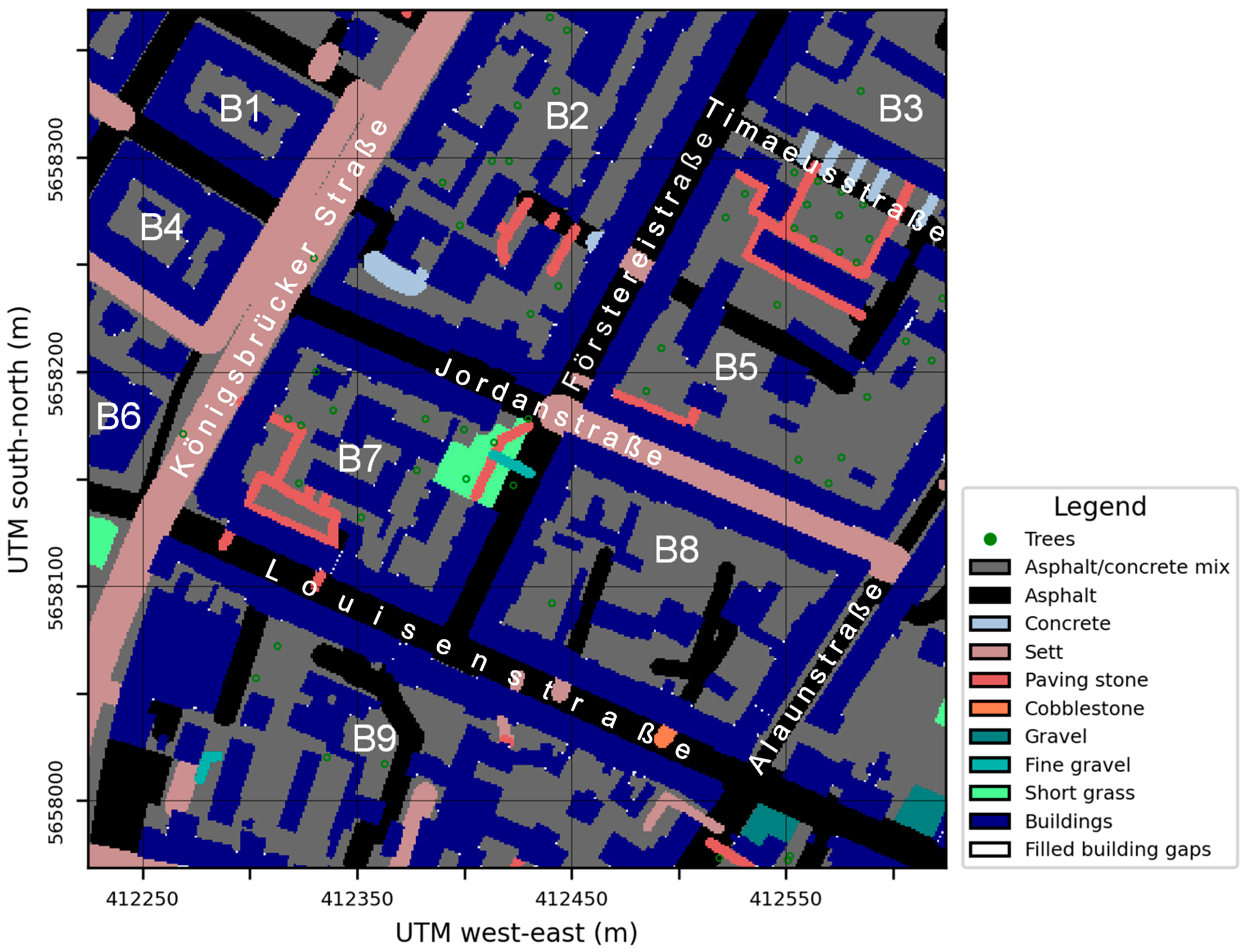
Figure 1. Static driver of the Dresden model area providing information on pavement and vegetation types as well as building geometry. The map shows the 400 m × 400 m child domain with a resolution of 1 m. Additionally labeled are the main streets and the different building blocks (B1–B9).
Atmosphere 16 01035 g001
Figure 2. Point density of the 10 min air temperature data of the Baseline simulation in the Dresden child domain at 1.5 m above ground. The black solid line represents the standard deviation σθ and the red dashed and dotted lines the median plus/minus σθ.
Atmosphere 16 01035 g002
Figure 3. Air temperature at 02:00 UTC in the Dresden child domain at 1.5 m above ground. In addition, the horizontal wind speed and direction at the same height are displayed using arrows, supplemented by building height in shades of gray and the trees’ crown diameter in magenta rings.
Atmosphere 16 01035 g003
Figure 4. Air temperature at 07:40 UTC in the Dresden child domain at 1.5 m above ground. In addition, the horizontal wind speed and direction at the same height are displayed using arrows, supplemented by building height in shades of gray and the trees’ crown diameter in magenta rings.
Atmosphere 16 01035 g004
Figure 5. Representativity Index (RI) over 24 h (144 timesteps) in the Dresden child domain for the measurement level of 1.5 m. RI values ≥ 90% are displayed by red shading, supplemented by building height in shades of gray and the trees’ crown diameter in green circles.
Atmosphere 16 01035 g005
Figure 6. Time series of the absolute (left y-axis) and relative (right y-axis) number of grid cells of the Baseline simulation evaluated over 24 h at different simulated sensor heights (zm) classified as representative of air temperature at 1.5 m. The total number of available (non-built-up) grid cells (Nmax) is depicted by the red dotted line. The relative number of representative grid cells (right y-axis) is given as the deviation from 100%, i.e., −70% means 30% are representative.
Atmosphere 16 01035 g006
Figure 7. Number of representative model cells in dependence on measuring height (zm), geostrophic wind (W2 and W3), and median building heights (B14 and B 17). The black line represents the Baseline scenario (Table 1). The additional Y-axis depicts the relative change in % compared with the sensor height of 1.5 m of the Baseline scenario.
Atmosphere 16 01035 g007
Figure 8. Representativity Index (RI) of the Baseline simulation for pedestrian-level air temperature evaluated over 24 h in the Dresden child domain for the simulated measurement height of 4.5 m. RI values ≥ 90% are displayed by red color shading, supplemented by building height in shades of gray and the trees’ crown diameter in green circles.
Atmosphere 16 01035 g008
Figure 9. Time series of the median of temperature differences between the pedestrian level of 1.5 m and zm = 4.5 m (also called stratification-induced measurement error). A neutral stratification is indicated by values around 0. A stable stratification is shown by positive values, and an unstable stratification is reflected by negative values. Additionally depicted are the temperature standard deviation (dotted lines) at the pedestrian level (1.5 m). Panel (a): sensitivity to large-scale wind speed. Panel (b): sensitivity to building height.
Atmosphere 16 01035 g009
Table 1. Table of the simulation setups used for sensitivity tests.
SimulationWind ForcingMedian Building Height
Baseline1 m/s20 m
W22 m/s20 m
W33 m/s20 m
B171 m/s17 m
B141 m/s14 m
Disclaimer/Publisher’s Note: The statements, opinions and data contained in all publications are solely those of the individual author(s) and contributor(s) and not of MDPI and/or the editor(s). MDPI and/or the editor(s) disclaim responsibility for any injury to people or property resulting from any ideas, methods, instructions or products referred to in the content.